Antisymmetrized random phase approximation for quasielastic
scattering in nuclear matter: Non-relativistic potentials

Abstract

Many-body techniques for the calculation of quasielastic nuclear matter response functions in the fully antisymmetrized random phase approximation on a Hartree-Fock basis are discussed in detail. The methods presented here allow for an accurate evaluation of the response functions with little numerical effort. Formulae are given for a generic non-relativistic potential parameterized in terms of meson exchanges; on the other hand, relativistic kinematical effects have been accounted for.

I Introduction

Quasielastic electron scattering on nuclei has been in the past years the subject of intense experimental [1, 2, 3] and theoretical (see, e. g., Refs. [4, 5, 6, 7, 8, 9, 10, 11, 12, 13, 14, 15, 16, 17]) investigations. The first aim of the theoretical studies is to test the available nuclear models; once the nuclear physics issues are well understood, one might hope to gain insight into other aspects of the problem, for instance by extracting with sufficient precision the nucleon form factors.

In principle, the quasifree regime makes one confident that the physical quantities of interest may be computed in a reliable way; in practice, also in this case one has to cope with considerable computational problems. Many diverse techniques have been employed in the literature. Each of them has its own relative merits and deficiencies and, in general, it would be highly desirable to be able to reach some degree of convergence in their outcomes.

In the following, we shall be concerned with Green’s function techniques, as introduced, e. g., in Ref. [18]. These methods can be, and have been, applied both to finite nuclei and nuclear matter, the choice being generally driven by the specific reaction and by the momentum regime of interest. Here, we shall focus on the nuclear matter, having in mind applications to electron scattering (that is, without the complications introduced by the reaction mechanism of hadronic probes) in a range from a few hundreds to several hundreds MeV/c of transferred momenta (where the quasielastic peak is sufficiently far from low-energy resonances and not too much affected by finite size effects). The use of nuclear matter reduces the computational load, thus allowing a more straightforward implementation of more sophisticated theoretical schemes: This makes easier to develop and test approximation methods that could then be utilized also for calculations in finite nuclei.

Let us now briefly browse the theoretical framework that we shall discuss in detail in the following sections.

A first choice one has to do in setting up the formalism concerns the treatment of relativistic effects. Trivial kinematical effects can be obviously rather important and can be included in a straightforward way. The treatment of dynamical effects is more delicate. Two main paths have been followed in the literature: Either using field theoretical methods (as done, e. g., in the Walecka model and its derivations [19]) or potential techniques (using, i. e., phenomenological potentials truncated at some order in the non-relativistic expansion). Here, we shall put ourselves on the second path, but, to contain the amount of material, we shall employ strictly non-relativistic potentials. The extensions necessary to include higher order relativistic terms will be discussed elsewhere (see, however, Refs. [13, 20, 21] for a few applications).

Next, one should choose the phenomenological input potential and, in connection with this choice, possibly the way of dealing with short-range correlations. All the formulae we are going to give in the following sections are based on a generic one-boson-exchange potential. They can thus be used both with a bare phenomenological interaction, — such as one of the Bonn potential variants, — or with a one-boson-exchange parameterization of a $G$-matrix generated from some potential. The use of an effective interaction derived from a $G$-matrix is a common way of including short-range correlations. One should be aware of possible problems due to the use of a local potential to fit non-local matrix elements. At least in a few cases discussed in the literature this does not appear to be a reason of concern [22, 23]. On the other hand, possible effects due to the specific quasielastic regime remain completely unexplored: Indeed, $G$-matrices employed in quasielastic calculations are usually generated using bound state boundary conditions, which make them real and practically energy independent, while, in general, they might be complex and energy dependent.

Once we have fixed the effective interaction, we can proceed to consider a hierarchy of approximation schemes.

The lowest order approximation is, of course, given by the free Fermi gas. Then, one may include mean field correlations at the Hartree-Fock (HF) level (or Brueckner-Hartree-Fock (BHF) if short-range correlations are accounted for). In nuclear matter a HF calculation can be done exactly without too many efforts. Nevertheless, we show how a quite accurate analytic approximation can be derived, since we shall need the method later to combine the HF and the random phase approximation (RPA) schemes. The latter is the last resummation technique to be discussed. It should be noticed that even in nuclear matter the calculation of the antisymmetrized RPA response functions is not trivial. Indeed, most calculations that are labeled “RPA” in the literature are actually performed in the so-called “ring approximation”, where only the direct contributions are kept: In this case, in nuclear matter one gets an algebraic equation. Here, we use the continued fraction (CF) technique to provide a semi-analytical estimate of the full RPA response (see Refs. [6] and [8] for alternative methods). Calculations with this method have been performed both in finite nuclei [4, 5] and in nuclear matter [24, 25, 13, 20], always truncating the CF expansion at first order, because of the difficulty of the numerical calculations. We have pushed the analytical calculation far enough to allow not only a fast and accurate estimate of the first order CF expansion, but also of the second order one. Since in the CF technique there is no general way of estimating the convergence of the series, this is the only way of getting a quantitative hold on the quality of the approximation. As noticed before, HF (and kinematical relativistic) effects can then be incorporated in the RPA calculation, yielding as the final approximation scheme a HF-RPA (or BHF-RPA) response function.

Of course, many diverse many-body contributions have been left out. It should however be noted that the classes of many-body diagrams discussed here, on the one hand already allow one to study many interesting features of the quasielastic response; on the other hand, the fact of having developed semi-analytical methods reduces to a minimum the computational efforts, thus making this formalism a good starting point for the study of other many-body effects.

The paper is organized as follows. In Section 2 the theoretical machinery is set up, discussing in separate subsections the treatment of relativistic kinematics and the free, HF and RPA responses. The intent of this paper is just to provide theoretical tools, so we do not attempt any discussion of the phenomenology of quasielastic scattering. On the other hand, in Section 3 calculations based on the formalism previously developed are shown, in order to test the convergence of the CF expansion and the importance of antisymmetrization. Finally, in the last Section we present a few concluding remarks.

II Response functions

Let us consider an infinite system of (possibly) interacting nucleons, at some density corresponding to a Fermi momentum $k_{F}$. For the kinetic energies of the nucleons we can choose either the relativistic or non-relativistic expressions, whereas we assume that the interactions take place through a non-relativistic potential. For the latter we take the following general form in momentum space

$$V(\mathchoice{{\hbox{\boldmath$\displaystyle k$}}}{{\hbox{\boldmath$\textstyle k$}}}{{\hbox{\boldmath$\scriptstyle k$}}}{{\hbox{\boldmath$\scriptscriptstyle k$}}}) = V_{0}(k)+V_{\tau}(k)\mathchoice{{\hbox{\boldmath$\displaystyle\tau$}}}{{\hbox{\boldmath$\textstyle\tau$}}}{{\hbox{\boldmath$\scriptstyle\tau$}}}{{\hbox{\boldmath$\scriptscriptstyle\tau$}}}_{1}\cdot\mathchoice{{\hbox{\boldmath$\displaystyle\tau$}}}{{\hbox{\boldmath$\textstyle\tau$}}}{{\hbox{\boldmath$\scriptstyle\tau$}}}{{\hbox{\boldmath$\scriptscriptstyle\tau$}}}_{2}+V_{\sigma}(k)\mathchoice{{\hbox{\boldmath$\displaystyle\sigma$}}}{{\hbox{\boldmath$\textstyle\sigma$}}}{{\hbox{\boldmath$\scriptstyle\sigma$}}}{{\hbox{\boldmath$\scriptscriptstyle\sigma$}}}_{1}\cdot\mathchoice{{\hbox{\boldmath$\displaystyle\sigma$}}}{{\hbox{\boldmath$\textstyle\sigma$}}}{{\hbox{\boldmath$\scriptstyle\sigma$}}}{{\hbox{\boldmath$\scriptscriptstyle\sigma$}}}_{2}+V_{\sigma\tau}(k)\mathchoice{{\hbox{\boldmath$\displaystyle\sigma$}}}{{\hbox{\boldmath$\textstyle\sigma$}}}{{\hbox{\boldmath$\scriptstyle\sigma$}}}{{\hbox{\boldmath$\scriptscriptstyle\sigma$}}}_{1}\cdot\mathchoice{{\hbox{\boldmath$\displaystyle\sigma$}}}{{\hbox{\boldmath$\textstyle\sigma$}}}{{\hbox{\boldmath$\scriptstyle\sigma$}}}{{\hbox{\boldmath$\scriptscriptstyle\sigma$}}}_{2}\ \mathchoice{{\hbox{\boldmath$\displaystyle\tau$}}}{{\hbox{\boldmath$\textstyle\tau$}}}{{\hbox{\boldmath$\scriptstyle\tau$}}}{{\hbox{\boldmath$\scriptscriptstyle\tau$}}}_{1}\cdot\mathchoice{{\hbox{\boldmath$\displaystyle\tau$}}}{{\hbox{\boldmath$\textstyle\tau$}}}{{\hbox{\boldmath$\scriptstyle\tau$}}}{{\hbox{\boldmath$\scriptscriptstyle\tau$}}}_{2}$$ (2)

$$\quad+V_{t}(k)S_{12}(\hat{\mathchoice{{\hbox{\boldmath$\displaystyle k$}}}{{\hbox{\boldmath$\textstyle k$}}}{{\hbox{\boldmath$\scriptstyle k$}}}{{\hbox{\boldmath$\scriptscriptstyle k$}}}})+V_{t\tau}(k)S_{12}(\hat{\mathchoice{{\hbox{\boldmath$\displaystyle k$}}}{{\hbox{\boldmath$\textstyle k$}}}{{\hbox{\boldmath$\scriptstyle k$}}}{{\hbox{\boldmath$\scriptscriptstyle k$}}}})\mathchoice{{\hbox{\boldmath$\displaystyle\tau$}}}{{\hbox{\boldmath$\textstyle\tau$}}}{{\hbox{\boldmath$\scriptstyle\tau$}}}{{\hbox{\boldmath$\scriptscriptstyle\tau$}}}_{1}\cdot\mathchoice{{\hbox{\boldmath$\displaystyle\tau$}}}{{\hbox{\boldmath$\textstyle\tau$}}}{{\hbox{\boldmath$\scriptstyle\tau$}}}{{\hbox{\boldmath$\scriptscriptstyle\tau$}}}_{2},$$

where $S_{12}$ is the standard tensor operator and $V_{\alpha}(k)$ represents the momentum space potential in channel $\alpha$. Here, we assume that $V_{\alpha}(k)$ has the general form of a static one-boson-exchange potential, so that in each spin-isospin channel it is given as a sum of contributions from different mesons, $V_{\alpha}\equiv\sum_{i}V_{\alpha}^{(i)}$. In the central channels ($0$, $\tau$, $\sigma$, $\sigma\tau$) the contribution from any meson can be expressed as the combination of a short-range (“$\delta$”) piece and a longer range (“momentum dependent”) piece:

$$V_{\delta}^{(i)}(k) = g_{\delta}^{(i)}\left(\frac{\Lambda_{i}^{2}-m_{i}^{2}}{\Lambda_{i}^{2}+k^{2}}\right)^{\ell}$$ (4)

$$V_{\text{MD}}^{(i)}(k) = g_{\text{MD}}^{(i)}\frac{m_{i}^{2}}{m_{i}^{2}+k^{2}}\left(\frac{\Lambda_{i}^{2}-m_{i}^{2}}{\Lambda_{i}^{2}+k^{2}}\right)^{\ell},\quad\ell=0,1,2,$$ (5)

whereas in the tensor channels ($t$, $t\tau$) is given by

$$V_{\text{TN}}^{(i)}(k)=g_{\text{TN}}^{(i)}\frac{k^{2}}{m_{i}^{2}+k^{2}}\left(\frac{\Lambda_{i}^{2}-m_{i}^{2}}{\Lambda_{i}^{2}+k^{2}}\right)^{\ell},\quad\ell=0,1,2.$$ (6)

In Eqs. (* ‣ II), $g_{\delta}^{(i)}$, $g_{\text{MD}}^{(i)}$ and $g_{\text{TN}}^{(i)}$ are the (dimensional) coupling constant of the $i$-th meson, $m_{i}$ is its mass and $\Lambda_{i}$ the cut-off; to be more general, we have allowed for a choice among potentials without form factors or with monopole or dipole form factors.

Our starting point [26, 27, 28] is given by the Galitskii-Migdal integral equation for the particle-hole (ph) four-point Green’s function,

$$G^{\text{ph}}_{\alpha\beta,\gamma\delta}(K+Q,K;P+Q,P)=-G_{\alpha\gamma}(P+Q)\,G_{\delta\beta}(P)\,(2\pi)^{4}\delta(K-P)$$ (7)

$$+iG_{\alpha\lambda}(K+Q)\,G_{\lambda^{\prime}\beta}(K)\int\frac{d^{4}T}{(2\pi)^{4}}\Gamma^{13}_{\lambda\lambda^{\prime},\mu\mu^{\prime}}(K+Q,K;T+Q,T)\,G^{\text{ph}}_{\mu\mu^{\prime},\gamma\delta}(T+Q,T;P+Q,P),$$ (8)

(9)

which is diagrammatically illustrated in Fig. 1. In (9), $G$ represents the exact one-body Green’s function, whereas $\Gamma^{13}$ is the irreducible vertex function in the ph channel.

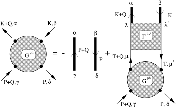
FIG. 1.: Diagrammatic representation of the Galitskii-Migdal integral equation for the ph Green’s function, $G^{\text{ph}}$; $\Gamma^{13}$ is the irreducible vertex function in the ph channel; the heavy lines represent the exact one-body Green’s functions.

Given $G^{\text{ph}}$ one can then define the polarization propagator

$$\Pi_{\alpha\beta,\gamma\delta}(Q) \equiv \Pi_{\alpha\beta,\gamma\delta}(q,\omega)$$ (10)

$$= i\int\frac{d^{4}P}{(2\pi)^{4}}\frac{d^{4}K}{(2\pi)^{4}}G^{\text{ph}}_{\alpha\beta,\gamma\delta}(K+Q,K;P+Q,P),$$ (11)

whose diagrammatic representation is displayed in Fig. 2. Note that for $\Pi(q,\omega)$ one cannot, in general, write down an integral (or algebraic) equation.

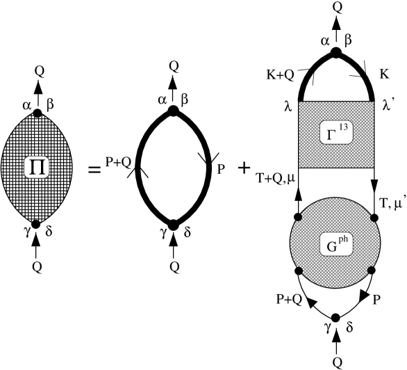
FIG. 2.: Diagrammatic representation of the polarization propagator $\Pi$ derived from the ph Green’s function $G^{\text{ph}}$.

In the case of electron scattering, one can define charge, — or longitudinal, — and magnetic, — or transverse, — polarization propagators:

$$\Pi^{I}_{\text{L}}(q,\omega)=\text{tr}[\hat{O}^{I}_{\text{L}}\hat{\Pi}(q,\omega)\hat{O}^{I}_{\text{L}}]$$ (13)

$$\Pi^{I}_{\text{T}}(q,\omega)=\sum_{ij}\Lambda_{ji}\Pi^{I}_{ij}(q,\omega),\qquad\Pi^{I}_{ij}(q,\omega)=\text{tr}[\hat{O}^{I}_{\text{T};i}\hat{\Pi}(q,\omega)\hat{O}^{I}_{\text{T};j}]$$ (14)

$$\phantom{\Pi^{I}_{\text{T}}(q,\omega)=\sum_{ij}\Lambda_{ji}\Pi^{I}_{ij}(q,\omega),}\qquad\,\Lambda_{ij}=(\delta_{ij}-\hat{\mathchoice{{\hbox{\boldmath$\displaystyle q$}}}{{\hbox{\boldmath$\textstyle q$}}}{{\hbox{\boldmath$\scriptstyle q$}}}{{\hbox{\boldmath$\scriptscriptstyle q$}}}}_{i}\hat{\mathchoice{{\hbox{\boldmath$\displaystyle q$}}}{{\hbox{\boldmath$\textstyle q$}}}{{\hbox{\boldmath$\scriptstyle q$}}}{{\hbox{\boldmath$\scriptscriptstyle q$}}}}_{j})/2,$$ (15)

where, for brevity, the dependence upon the spin-isospin indices has been represented in matrix form, introducing hats where appropriate. In (2), $I$ labels the isospin channel and the longitudinal and transverse vertex operators are given as follows:

$$\left\{\begin{array}[]{l}\hat{O}^{I=0}_{\text{L}}=1/2\\ \hat{O}^{I=1}_{\text{L}}=\tau_{3}/2\end{array}\right.\qquad\qquad\left\{\begin{array}[]{l}\hat{O}^{I=0}_{\text{T};i}=\sigma_{i}/2\\ \hat{O}^{I=1}_{\text{T};i}=\sigma_{i}\tau_{3}/2.\end{array}\right.$$ (16)

The quantity of interest here is the imaginary part of $\Pi_{\text{L,T}}(q,\omega)$, since the inelastic scattering cross section, — where the momentum $q$ and the energy $\omega$ have been transferred to the nucleus, — is a linear combination of $\text{Im}\Pi_{\text{L}}$ and $\text{Im}\Pi_{\text{T}}$. It is then customary to define longitudinal and transverse response functions

$$R_{\text{L,T}}(q,\omega)=R^{I=0}_{\text{L,T}}(q,\omega)+R^{I=1}_{\text{L,T}}(q,\omega),$$ (17)

which are related to $\Pi_{\text{L,T}}$ by

$$R^{I}_{\text{L,T}}(q,\omega) = -\frac{V}{\pi}{f^{(I)}_{\text{L,T}}}^{2}(q,\omega)\text{Im}\Pi^{I}_{\text{L,T}}(q,\omega)$$ (18)

$$= -\frac{3\pi A}{2k_{F}^{3}}{f^{(I)}_{\text{L,T}}}^{2}(q,\omega)\text{Im}\Pi^{I}_{\text{L,T}}(q,\omega),$$ (19)

where $V$ is the volume, $A$ the mass number and ${f^{(I)}_{\text{L,T}}}^{2}$ contain the squared electromagnetic form factors of the nucleon.

A Non-relativistic vs relativistic kinematics

The response functions introduced above have been defined as functions of the momentum transfer $q$ and of the energy transfer $\omega$. Actually, it is possible, — and convenient, — to define a scaling variable $\psi$, which combines $q$ and $\omega$: This variable is such that the free responses in the non-Pauli-blocked region ($q>2k_{F}$) can be expressed in terms of the unique variable $\psi$ (apart from $q$-dependent multiplicative factors). We shall see that even in the Pauli-blocked region and for an interacting system it is convenient to use the pair of variables ($q$,$\psi$) instead of ($q$,$\omega$).

Besides the obvious advantages related to the use of a scaling variable, there is another good reason for expressing the responses in terms of $\psi$: In fact, in this way one can define response functions that are independent of the form chosen for the nucleon kinetic energy. To be more specific: Starting from either a non-relativistic or a relativistic Fermi gas, one is always lead to the same expressions for the responses in terms of ($q$,$\psi$); to be different in the two cases is, of course, the definition of $\psi$ in terms of ($q$,$\omega$).

We shall see in the following subsections that the energy denominators of the free nucleon propagators, appearing in the Feynman diagrams for the response functions, can always be written as $\omega-\epsilon^{(0)}_{\mathchoice{{\hbox{\boldmath$\displaystyle k$}}}{{\hbox{\boldmath$\textstyle k$}}}{{\hbox{\boldmath$\scriptstyle k$}}}{{\hbox{\boldmath$\scriptscriptstyle k$}}}+\mathchoice{{\hbox{\boldmath$\displaystyle q$}}}{{\hbox{\boldmath$\textstyle q$}}}{{\hbox{\boldmath$\scriptstyle q$}}}{{\hbox{\boldmath$\scriptscriptstyle q$}}}}+\epsilon^{(0)}_{\mathchoice{{\hbox{\boldmath$\displaystyle k$}}}{{\hbox{\boldmath$\textstyle k$}}}{{\hbox{\boldmath$\scriptstyle k$}}}{{\hbox{\boldmath$\scriptscriptstyle k$}}}}$, where $\epsilon^{(0)}_{\mathchoice{{\hbox{\boldmath$\displaystyle k$}}}{{\hbox{\boldmath$\textstyle k$}}}{{\hbox{\boldmath$\scriptstyle k$}}}{{\hbox{\boldmath$\scriptscriptstyle k$}}}}$ is the kinetic energy of a nucleon of momentum $k$ and $k<k_{F}$. In the non-relativistic case, one finds

$$\omega-\epsilon^{(0)\text{nr}}_{\mathchoice{{\hbox{\boldmath$\displaystyle k$}}}{{\hbox{\boldmath$\textstyle k$}}}{{\hbox{\boldmath$\scriptstyle k$}}}{{\hbox{\boldmath$\scriptscriptstyle k$}}}+\mathchoice{{\hbox{\boldmath$\displaystyle q$}}}{{\hbox{\boldmath$\textstyle q$}}}{{\hbox{\boldmath$\scriptstyle q$}}}{{\hbox{\boldmath$\scriptscriptstyle q$}}}}+\epsilon^{(0)\text{nr}}_{\mathchoice{{\hbox{\boldmath$\displaystyle k$}}}{{\hbox{\boldmath$\textstyle k$}}}{{\hbox{\boldmath$\scriptstyle k$}}}{{\hbox{\boldmath$\scriptscriptstyle k$}}}}=\frac{qk_{F}}{m_{N}}\left(\psi_{\text{nr}}-\hat{\mathchoice{{\hbox{\boldmath$\displaystyle q$}}}{{\hbox{\boldmath$\textstyle q$}}}{{\hbox{\boldmath$\scriptstyle q$}}}{{\hbox{\boldmath$\scriptscriptstyle q$}}}}\cdot\frac{\mathchoice{{\hbox{\boldmath$\displaystyle k$}}}{{\hbox{\boldmath$\textstyle k$}}}{{\hbox{\boldmath$\scriptstyle k$}}}{{\hbox{\boldmath$\scriptscriptstyle k$}}}}{k_{F}}\right),$$ (20)

where

$$\psi_{\text{nr}}=\frac{1}{k_{F}}\left(\frac{\omega m_{N}}{q}-\frac{q}{2}\right)$$ (21)

is the standard scaling variable of the non-relativistic Fermi gas and $m_{N}$ the nucleon mass.

In the relativistic case, in Ref. [29] it had been shown that at the pole it is a very good approximation to use Eq. (20) substituting $\psi_{\text{nr}}$ with

$$\psi_{\text{r}}=\frac{1}{k_{F}}\left[\frac{\omega m_{N}(1+\omega/2m_{N})}{q}-\frac{q}{2}\right]$$ (22)

and multiplying the free response by the Jacobian of the transformation, $1+\omega/m_{N}$.

However, in the calculation of higher order (RPA) contributions, also the real part of the energy denominators comes into play and one has to check the quality of the approximation far from the pole. With some algebra, — and assuming $k^{2}/m_{N}^{2}<<1$, — one can write

$$\omega-\epsilon^{(0)\text{r}}_{\mathchoice{{\hbox{\boldmath$\displaystyle k$}}}{{\hbox{\boldmath$\textstyle k$}}}{{\hbox{\boldmath$\scriptstyle k$}}}{{\hbox{\boldmath$\scriptscriptstyle k$}}}+\mathchoice{{\hbox{\boldmath$\displaystyle q$}}}{{\hbox{\boldmath$\textstyle q$}}}{{\hbox{\boldmath$\scriptstyle q$}}}{{\hbox{\boldmath$\scriptscriptstyle q$}}}}+\epsilon^{(0)\text{r}}_{\mathchoice{{\hbox{\boldmath$\displaystyle k$}}}{{\hbox{\boldmath$\textstyle k$}}}{{\hbox{\boldmath$\scriptstyle k$}}}{{\hbox{\boldmath$\scriptscriptstyle k$}}}} \cong \frac{qk_{F}}{m_{N}}\frac{\psi_{r}-\hat{\mathchoice{{\hbox{\boldmath$\displaystyle q$}}}{{\hbox{\boldmath$\textstyle q$}}}{{\hbox{\boldmath$\scriptstyle q$}}}{{\hbox{\boldmath$\scriptscriptstyle q$}}}}\cdot\mathchoice{{\hbox{\boldmath$\displaystyle k$}}}{{\hbox{\boldmath$\textstyle k$}}}{{\hbox{\boldmath$\scriptstyle k$}}}{{\hbox{\boldmath$\scriptscriptstyle k$}}}/k_{F}}{\displaystyle\frac{1}{\displaystyle 2}\left(1+\frac{\omega}{\displaystyle m_{N}}+\sqrt{1+\frac{q^{2}+2\mathchoice{{\hbox{\boldmath$\displaystyle q$}}}{{\hbox{\boldmath$\textstyle q$}}}{{\hbox{\boldmath$\scriptstyle q$}}}{{\hbox{\boldmath$\scriptscriptstyle q$}}}\cdot{k}}{\displaystyle m_{N}^{2}}}\right)}$$ (23)

$$\cong \frac{qk_{F}}{m_{N}}\frac{\psi_{r}-\hat{\mathchoice{{\hbox{\boldmath$\displaystyle q$}}}{{\hbox{\boldmath$\textstyle q$}}}{{\hbox{\boldmath$\scriptstyle q$}}}{{\hbox{\boldmath$\scriptscriptstyle q$}}}}\cdot\mathchoice{{\hbox{\boldmath$\displaystyle k$}}}{{\hbox{\boldmath$\textstyle k$}}}{{\hbox{\boldmath$\scriptstyle k$}}}{{\hbox{\boldmath$\scriptscriptstyle k$}}}/k_{F}}{1+\omega/m_{N}},$$ (24)

where, in the last passage, we have replaced the square root with its value at the pole. In Fig. 3, we display the real part of the free polarization propagator (defined in the following subsection) using the exact relativistic dispersion relation and the prescription of Eq. (24) at $q=500$ MeV/c and 1 GeV/c as a function of $\omega$. We note that the agreement between the two ways of calculating $\text{Re}\Pi^{(0)}$ is quite good at both momenta.

FIG. 3.: $\text{Re}\Pi^{(0)}$ at $q=500$ MeV/c and 1000 MeV/c as a function of the energy transfer: Using the exact relativistic kinetic energies (solid) and the approximation discussed in the text (dash); $k_{F}=195$ MeV/c.

Eq. (24) provides an approximation for the free ph propagator: A prescription to get the (kinematically) relativistic polarization propagators at any order in the RPA expansion (see Section II D) can easily be obtained by noting that $\Pi^{(n)}$, — the $n$-th order contribution to the RPA chain, — contains $n+1$ ph propagators; then, one has

$$\Pi^{(n)\text{r}}(q,\omega)=\left(1+\frac{\omega}{m_{N}}\right)^{n+1}\Pi^{(n)\text{nr}}(q,\omega(1+\omega/2m_{N})).$$ (26)

Actually, all the response functions derived below are expressed in terms of a generic scaling variable $\psi$, as $\Pi^{(n)}(q,\psi)$: One can then get the non-relativistic response by using the (exact) expression (21) for $\psi$ and the relativistic response by using the (approximate) form (22) and multiplying each polarization propagator by the appropriate power of $1+\omega/m_{N}$, i. e.

$$\Pi^{(n)\text{r}}(q,\omega)=\left(1+\frac{\omega}{m_{N}}\right)^{n+1}\Pi^{(n)\text{nr}}(q,\psi_{\text{r}}).$$ (27)

Note that in the calculations of Refs. [13, 20] only an overall Jacobian factor, $1+\omega/m_{N}$, has been applied to the RPA response functions.

B Free response

Although the free Fermi gas response function is a subject for textbooks (see, e. g., Ref. [18]), it is useful to derive it here using a slightly different approach, since it illustrates at the simplest level the method we have adopted to overcome a major technical difficulty one meets in nuclear matter calculations, — namely the presence of $\theta$ functions, which considerably complicate analytic integrations. As a side effect, also the calculation of $\Pi^{(0)}$ comes out much more compact than in standard treatments.

From Eqs. (2) and (16), one immediately finds that

$$\Pi^{(0)}_{\text{L};I=0}=\Pi^{(0)}_{\text{L};I=1}=\Pi^{(0)}_{\text{T};I=0}=\Pi^{(0)}_{\text{T};I=1}\equiv\Pi^{(0)},$$ (28)

where, following (9) and (11) we have defined

$$\Pi^{(0)}(q,\omega)=\int\frac{d\mathchoice{{\hbox{\boldmath$\displaystyle k$}}}{{\hbox{\boldmath$\textstyle k$}}}{{\hbox{\boldmath$\scriptstyle k$}}}{{\hbox{\boldmath$\scriptscriptstyle k$}}}}{(2\pi)^{3}}G^{(0)}_{\text{ph}}(\mathchoice{{\hbox{\boldmath$\displaystyle k$}}}{{\hbox{\boldmath$\textstyle k$}}}{{\hbox{\boldmath$\scriptstyle k$}}}{{\hbox{\boldmath$\scriptscriptstyle k$}}},\mathchoice{{\hbox{\boldmath$\displaystyle q$}}}{{\hbox{\boldmath$\textstyle q$}}}{{\hbox{\boldmath$\scriptstyle q$}}}{{\hbox{\boldmath$\scriptscriptstyle q$}}};\omega),$$ (29)

having set

$$G^{(0)}_{\text{ph}}(\mathchoice{{\hbox{\boldmath$\displaystyle k$}}}{{\hbox{\boldmath$\textstyle k$}}}{{\hbox{\boldmath$\scriptstyle k$}}}{{\hbox{\boldmath$\scriptscriptstyle k$}}},\mathchoice{{\hbox{\boldmath$\displaystyle q$}}}{{\hbox{\boldmath$\textstyle q$}}}{{\hbox{\boldmath$\scriptstyle q$}}}{{\hbox{\boldmath$\scriptscriptstyle q$}}};\omega)=-i\int\frac{dk_{0}}{2\pi}G^{(0)}(\mathchoice{{\hbox{\boldmath$\displaystyle k$}}}{{\hbox{\boldmath$\textstyle k$}}}{{\hbox{\boldmath$\scriptstyle k$}}}{{\hbox{\boldmath$\scriptscriptstyle k$}}}+\mathchoice{{\hbox{\boldmath$\displaystyle q$}}}{{\hbox{\boldmath$\textstyle q$}}}{{\hbox{\boldmath$\scriptstyle q$}}}{{\hbox{\boldmath$\scriptscriptstyle q$}}},k_{0}+\omega)G^{(0)}(k,k_{0}),$$ (30)

$G^{(0)}(k,k_{0})$ being the free one-body propagator

$$G^{(0)}(k,k_{0})=\frac{\theta(k-k_{F})}{k_{0}-\epsilon^{(0)}_{\mathchoice{{\hbox{\boldmath$\displaystyle k$}}}{{\hbox{\boldmath$\textstyle k$}}}{{\hbox{\boldmath$\scriptstyle k$}}}{{\hbox{\boldmath$\scriptscriptstyle k$}}}}+i\eta}+\frac{\theta(k_{F}-k)}{k_{0}-\epsilon^{(0)}_{\mathchoice{{\hbox{\boldmath$\displaystyle k$}}}{{\hbox{\boldmath$\textstyle k$}}}{{\hbox{\boldmath$\scriptstyle k$}}}{{\hbox{\boldmath$\scriptscriptstyle k$}}}}-i\eta}.$$ (31)

The integration over $k_{0}$ in (30) is straightforward, yielding

$$G^{(0)}_{\text{ph}}(\mathchoice{{\hbox{\boldmath$\displaystyle k$}}}{{\hbox{\boldmath$\textstyle k$}}}{{\hbox{\boldmath$\scriptstyle k$}}}{{\hbox{\boldmath$\scriptscriptstyle k$}}},\mathchoice{{\hbox{\boldmath$\displaystyle q$}}}{{\hbox{\boldmath$\textstyle q$}}}{{\hbox{\boldmath$\scriptstyle q$}}}{{\hbox{\boldmath$\scriptscriptstyle q$}}};\omega)=\frac{\theta(k_{F}-k)\theta(|\mathchoice{{\hbox{\boldmath$\displaystyle k$}}}{{\hbox{\boldmath$\textstyle k$}}}{{\hbox{\boldmath$\scriptstyle k$}}}{{\hbox{\boldmath$\scriptscriptstyle k$}}}+\mathchoice{{\hbox{\boldmath$\displaystyle q$}}}{{\hbox{\boldmath$\textstyle q$}}}{{\hbox{\boldmath$\scriptstyle q$}}}{{\hbox{\boldmath$\scriptscriptstyle q$}}}|-k_{F})}{\omega-\epsilon^{(0)}_{\mathchoice{{\hbox{\boldmath$\displaystyle k$}}}{{\hbox{\boldmath$\textstyle k$}}}{{\hbox{\boldmath$\scriptstyle k$}}}{{\hbox{\boldmath$\scriptscriptstyle k$}}}+\mathchoice{{\hbox{\boldmath$\displaystyle q$}}}{{\hbox{\boldmath$\textstyle q$}}}{{\hbox{\boldmath$\scriptstyle q$}}}{{\hbox{\boldmath$\scriptscriptstyle q$}}}}+\epsilon^{(0)}_{\mathchoice{{\hbox{\boldmath$\displaystyle k$}}}{{\hbox{\boldmath$\textstyle k$}}}{{\hbox{\boldmath$\scriptstyle k$}}}{{\hbox{\boldmath$\scriptscriptstyle k$}}}}+i\eta}+\frac{\theta(k-k_{F})\theta(k_{F}-|\mathchoice{{\hbox{\boldmath$\displaystyle k$}}}{{\hbox{\boldmath$\textstyle k$}}}{{\hbox{\boldmath$\scriptstyle k$}}}{{\hbox{\boldmath$\scriptscriptstyle k$}}}+\mathchoice{{\hbox{\boldmath$\displaystyle q$}}}{{\hbox{\boldmath$\textstyle q$}}}{{\hbox{\boldmath$\scriptstyle q$}}}{{\hbox{\boldmath$\scriptscriptstyle q$}}}|)}{-\omega+\epsilon^{(0)}_{\mathchoice{{\hbox{\boldmath$\displaystyle k$}}}{{\hbox{\boldmath$\textstyle k$}}}{{\hbox{\boldmath$\scriptstyle k$}}}{{\hbox{\boldmath$\scriptscriptstyle k$}}}+\mathchoice{{\hbox{\boldmath$\displaystyle q$}}}{{\hbox{\boldmath$\textstyle q$}}}{{\hbox{\boldmath$\scriptstyle q$}}}{{\hbox{\boldmath$\scriptscriptstyle q$}}}}-\epsilon^{(0)}_{\mathchoice{{\hbox{\boldmath$\displaystyle k$}}}{{\hbox{\boldmath$\textstyle k$}}}{{\hbox{\boldmath$\scriptstyle k$}}}{{\hbox{\boldmath$\scriptscriptstyle k$}}}}+i\eta},$$ (32)

which, inserted back into (29), would give the standard definition of $\Pi^{(0)}$. Instead, let us rewrite $G^{(0)}_{\text{ph}}$ as

$$G^{(0)}_{\text{ph}}(\mathchoice{{\hbox{\boldmath$\displaystyle k$}}}{{\hbox{\boldmath$\textstyle k$}}}{{\hbox{\boldmath$\scriptstyle k$}}}{{\hbox{\boldmath$\scriptscriptstyle k$}}},\mathchoice{{\hbox{\boldmath$\displaystyle q$}}}{{\hbox{\boldmath$\textstyle q$}}}{{\hbox{\boldmath$\scriptstyle q$}}}{{\hbox{\boldmath$\scriptscriptstyle q$}}};\omega) = \frac{\theta(k_{F}-k)\theta(|\mathchoice{{\hbox{\boldmath$\displaystyle k$}}}{{\hbox{\boldmath$\textstyle k$}}}{{\hbox{\boldmath$\scriptstyle k$}}}{{\hbox{\boldmath$\scriptscriptstyle k$}}}+\mathchoice{{\hbox{\boldmath$\displaystyle q$}}}{{\hbox{\boldmath$\textstyle q$}}}{{\hbox{\boldmath$\scriptstyle q$}}}{{\hbox{\boldmath$\scriptscriptstyle q$}}}|-k_{F})}{\omega-\epsilon^{(0)}_{\mathchoice{{\hbox{\boldmath$\displaystyle k$}}}{{\hbox{\boldmath$\textstyle k$}}}{{\hbox{\boldmath$\scriptstyle k$}}}{{\hbox{\boldmath$\scriptscriptstyle k$}}}+\mathchoice{{\hbox{\boldmath$\displaystyle q$}}}{{\hbox{\boldmath$\textstyle q$}}}{{\hbox{\boldmath$\scriptstyle q$}}}{{\hbox{\boldmath$\scriptscriptstyle q$}}}}+\epsilon^{(0)}_{\mathchoice{{\hbox{\boldmath$\displaystyle k$}}}{{\hbox{\boldmath$\textstyle k$}}}{{\hbox{\boldmath$\scriptstyle k$}}}{{\hbox{\boldmath$\scriptscriptstyle k$}}}}+i\eta}+\frac{\theta(k-k_{F})\theta(k_{F}-|\mathchoice{{\hbox{\boldmath$\displaystyle k$}}}{{\hbox{\boldmath$\textstyle k$}}}{{\hbox{\boldmath$\scriptstyle k$}}}{{\hbox{\boldmath$\scriptscriptstyle k$}}}+\mathchoice{{\hbox{\boldmath$\displaystyle q$}}}{{\hbox{\boldmath$\textstyle q$}}}{{\hbox{\boldmath$\scriptstyle q$}}}{{\hbox{\boldmath$\scriptscriptstyle q$}}}|)}{-\omega+\epsilon^{(0)}_{\mathchoice{{\hbox{\boldmath$\displaystyle k$}}}{{\hbox{\boldmath$\textstyle k$}}}{{\hbox{\boldmath$\scriptstyle k$}}}{{\hbox{\boldmath$\scriptscriptstyle k$}}}+\mathchoice{{\hbox{\boldmath$\displaystyle q$}}}{{\hbox{\boldmath$\textstyle q$}}}{{\hbox{\boldmath$\scriptstyle q$}}}{{\hbox{\boldmath$\scriptscriptstyle q$}}}}-\epsilon^{(0)}_{\mathchoice{{\hbox{\boldmath$\displaystyle k$}}}{{\hbox{\boldmath$\textstyle k$}}}{{\hbox{\boldmath$\scriptstyle k$}}}{{\hbox{\boldmath$\scriptscriptstyle k$}}}}+i\eta}$$ (34)

$$+\frac{\theta(k_{F}-k)\theta(k_{F}-|\mathchoice{{\hbox{\boldmath$\displaystyle k$}}}{{\hbox{\boldmath$\textstyle k$}}}{{\hbox{\boldmath$\scriptstyle k$}}}{{\hbox{\boldmath$\scriptscriptstyle k$}}}+\mathchoice{{\hbox{\boldmath$\displaystyle q$}}}{{\hbox{\boldmath$\textstyle q$}}}{{\hbox{\boldmath$\scriptstyle q$}}}{{\hbox{\boldmath$\scriptscriptstyle q$}}}|)}{\omega-\epsilon^{(0)}_{\mathchoice{{\hbox{\boldmath$\displaystyle k$}}}{{\hbox{\boldmath$\textstyle k$}}}{{\hbox{\boldmath$\scriptstyle k$}}}{{\hbox{\boldmath$\scriptscriptstyle k$}}}+\mathchoice{{\hbox{\boldmath$\displaystyle q$}}}{{\hbox{\boldmath$\textstyle q$}}}{{\hbox{\boldmath$\scriptstyle q$}}}{{\hbox{\boldmath$\scriptscriptstyle q$}}}}+\epsilon^{(0)}_{\mathchoice{{\hbox{\boldmath$\displaystyle k$}}}{{\hbox{\boldmath$\textstyle k$}}}{{\hbox{\boldmath$\scriptstyle k$}}}{{\hbox{\boldmath$\scriptscriptstyle k$}}}}+i\eta_{\omega}}+\frac{\theta(k_{F}-k)\theta(k_{F}-|\mathchoice{{\hbox{\boldmath$\displaystyle k$}}}{{\hbox{\boldmath$\textstyle k$}}}{{\hbox{\boldmath$\scriptstyle k$}}}{{\hbox{\boldmath$\scriptscriptstyle k$}}}+\mathchoice{{\hbox{\boldmath$\displaystyle q$}}}{{\hbox{\boldmath$\textstyle q$}}}{{\hbox{\boldmath$\scriptstyle q$}}}{{\hbox{\boldmath$\scriptscriptstyle q$}}}|)}{-\omega+\epsilon^{(0)}_{\mathchoice{{\hbox{\boldmath$\displaystyle k$}}}{{\hbox{\boldmath$\textstyle k$}}}{{\hbox{\boldmath$\scriptstyle k$}}}{{\hbox{\boldmath$\scriptscriptstyle k$}}}+\mathchoice{{\hbox{\boldmath$\displaystyle q$}}}{{\hbox{\boldmath$\textstyle q$}}}{{\hbox{\boldmath$\scriptstyle q$}}}{{\hbox{\boldmath$\scriptscriptstyle q$}}}}-\epsilon^{(0)}_{\mathchoice{{\hbox{\boldmath$\displaystyle k$}}}{{\hbox{\boldmath$\textstyle k$}}}{{\hbox{\boldmath$\scriptstyle k$}}}{{\hbox{\boldmath$\scriptscriptstyle k$}}}}-i\eta_{\omega}},$$

having added and subtracted the quantity in the second line, where we have set $\eta_{\omega}=\text{sign}(\omega)\eta$. A few algebraic manipulations then yield

$$G^{(0)}_{\text{ph}}(\mathchoice{{\hbox{\boldmath$\displaystyle k$}}}{{\hbox{\boldmath$\textstyle k$}}}{{\hbox{\boldmath$\scriptstyle k$}}}{{\hbox{\boldmath$\scriptscriptstyle k$}}},\mathchoice{{\hbox{\boldmath$\displaystyle q$}}}{{\hbox{\boldmath$\textstyle q$}}}{{\hbox{\boldmath$\scriptstyle q$}}}{{\hbox{\boldmath$\scriptscriptstyle q$}}};\omega)=\frac{\theta(k_{F}-k)-\theta(k_{F}-|\mathchoice{{\hbox{\boldmath$\displaystyle k$}}}{{\hbox{\boldmath$\textstyle k$}}}{{\hbox{\boldmath$\scriptstyle k$}}}{{\hbox{\boldmath$\scriptscriptstyle k$}}}+\mathchoice{{\hbox{\boldmath$\displaystyle q$}}}{{\hbox{\boldmath$\textstyle q$}}}{{\hbox{\boldmath$\scriptstyle q$}}}{{\hbox{\boldmath$\scriptscriptstyle q$}}}|)}{\omega-\epsilon^{(0)}_{\mathchoice{{\hbox{\boldmath$\displaystyle k$}}}{{\hbox{\boldmath$\textstyle k$}}}{{\hbox{\boldmath$\scriptstyle k$}}}{{\hbox{\boldmath$\scriptscriptstyle k$}}}+\mathchoice{{\hbox{\boldmath$\displaystyle q$}}}{{\hbox{\boldmath$\textstyle q$}}}{{\hbox{\boldmath$\scriptstyle q$}}}{{\hbox{\boldmath$\scriptscriptstyle q$}}}}+\epsilon^{(0)}_{\mathchoice{{\hbox{\boldmath$\displaystyle k$}}}{{\hbox{\boldmath$\textstyle k$}}}{{\hbox{\boldmath$\scriptstyle k$}}}{{\hbox{\boldmath$\scriptscriptstyle k$}}}}+i\eta_{\omega}}.$$ (35)

Hence, from (29) one gets

$$\Pi^{(0)}(q,\omega) = \int\frac{d\mathchoice{{\hbox{\boldmath$\displaystyle k$}}}{{\hbox{\boldmath$\textstyle k$}}}{{\hbox{\boldmath$\scriptstyle k$}}}{{\hbox{\boldmath$\scriptscriptstyle k$}}}}{(2\pi)^{3}}\theta(k_{F}-k)\left[\frac{1}{\omega-\epsilon^{(0)}_{\mathchoice{{\hbox{\boldmath$\displaystyle k$}}}{{\hbox{\boldmath$\textstyle k$}}}{{\hbox{\boldmath$\scriptstyle k$}}}{{\hbox{\boldmath$\scriptscriptstyle k$}}}+\mathchoice{{\hbox{\boldmath$\displaystyle q$}}}{{\hbox{\boldmath$\textstyle q$}}}{{\hbox{\boldmath$\scriptstyle q$}}}{{\hbox{\boldmath$\scriptscriptstyle q$}}}}+\epsilon^{(0)}_{\mathchoice{{\hbox{\boldmath$\displaystyle k$}}}{{\hbox{\boldmath$\textstyle k$}}}{{\hbox{\boldmath$\scriptstyle k$}}}{{\hbox{\boldmath$\scriptscriptstyle k$}}}}+i\eta_{\omega}}+\frac{1}{-\omega-\epsilon^{(0)}_{\mathchoice{{\hbox{\boldmath$\displaystyle k$}}}{{\hbox{\boldmath$\textstyle k$}}}{{\hbox{\boldmath$\scriptstyle k$}}}{{\hbox{\boldmath$\scriptscriptstyle k$}}}+\mathchoice{{\hbox{\boldmath$\displaystyle q$}}}{{\hbox{\boldmath$\textstyle q$}}}{{\hbox{\boldmath$\scriptstyle q$}}}{{\hbox{\boldmath$\scriptscriptstyle q$}}}}+\epsilon^{(0)}_{\mathchoice{{\hbox{\boldmath$\displaystyle k$}}}{{\hbox{\boldmath$\textstyle k$}}}{{\hbox{\boldmath$\scriptstyle k$}}}{{\hbox{\boldmath$\scriptscriptstyle k$}}}}-i\eta_{\omega}}\right]$$ (36)

$$= \frac{m_{N}}{q}\frac{k_{F}^{2}}{(2\pi)^{2}}\left[{\cal Q}^{(0)}(\psi)-{\cal Q}^{(0)}(\psi+\bar{q})\right].$$ (37)

Note that only one $\theta$ function forcing $k$ below $k_{F}$ is left, Pauli blocking being enforced by cancellations between the energy denominators. In (37), we have introduced $\bar{q}=q/k_{F}$ and the adimensional function

$${\cal Q}^{(0)}(\psi)=\frac{1}{2}\int_{-1}^{1}dy\frac{1-y^{2}}{\psi-y+i\eta_{\omega}},$$ (38)

which is easily evaluated, yielding

$$\text{Re}{\cal Q}^{(0)}(\psi) = \psi+\frac{1}{2}(1-\psi^{2})\text{ln}\left|\frac{1+\psi}{1-\psi}\right|=\frac{2}{3}[Q_{0}(\psi)-Q_{2}(\psi)]$$ (40)

$$\text{Im}{\cal Q}^{(0)}(\psi) = -\text{sign}(\omega)\theta(1-\psi^{2})\frac{\pi}{2}(1-\psi^{2})=-\text{sign}(\omega)\theta(1-\psi^{2})\frac{\pi}{3}[P_{0}(\psi)-P_{2}(\psi)],$$ (41)

where $P_{n}$ and $Q_{n}$ are Legendre polynomials and Legendre functions of second kind, respectively.

C Hartree-Fock response

The HF polarization propagator in nuclear matter is obtained by dressing the one-body propagators appearing in $\Pi^{(0)}$ with the first order self-energy $\Sigma^{(1)}$, so that one can follow essentially the same derivation of the previous subsection. The spin-isospin matrix elements are the same as for the free response, yielding

$$\Pi^{\text{HF}}_{\text{L};I=0}=\Pi^{\text{HF}}_{\text{L};I=1}=\Pi^{\text{HF}}_{\text{T};I=0}=\Pi^{\text{HF}}_{\text{T};I=1}\equiv\Pi^{\text{HF}},$$ (42)

where

$$\Pi^{\text{HF}}(q,\omega)=\int\frac{d\mathchoice{{\hbox{\boldmath$\displaystyle k$}}}{{\hbox{\boldmath$\textstyle k$}}}{{\hbox{\boldmath$\scriptstyle k$}}}{{\hbox{\boldmath$\scriptscriptstyle k$}}}}{(2\pi)^{3}}\theta(k_{F}-k)\left[\frac{1}{\omega-\epsilon^{(1)}_{\mathchoice{{\hbox{\boldmath$\displaystyle k$}}}{{\hbox{\boldmath$\textstyle k$}}}{{\hbox{\boldmath$\scriptstyle k$}}}{{\hbox{\boldmath$\scriptscriptstyle k$}}}+\mathchoice{{\hbox{\boldmath$\displaystyle q$}}}{{\hbox{\boldmath$\textstyle q$}}}{{\hbox{\boldmath$\scriptstyle q$}}}{{\hbox{\boldmath$\scriptscriptstyle q$}}}}+\epsilon^{(1)}_{\mathchoice{{\hbox{\boldmath$\displaystyle k$}}}{{\hbox{\boldmath$\textstyle k$}}}{{\hbox{\boldmath$\scriptstyle k$}}}{{\hbox{\boldmath$\scriptscriptstyle k$}}}}+i\eta_{\omega}}+\frac{1}{-\omega-\epsilon^{(0)}_{\mathchoice{{\hbox{\boldmath$\displaystyle k$}}}{{\hbox{\boldmath$\textstyle k$}}}{{\hbox{\boldmath$\scriptstyle k$}}}{{\hbox{\boldmath$\scriptscriptstyle k$}}}+\mathchoice{{\hbox{\boldmath$\displaystyle q$}}}{{\hbox{\boldmath$\textstyle q$}}}{{\hbox{\boldmath$\scriptstyle q$}}}{{\hbox{\boldmath$\scriptscriptstyle q$}}}}+\epsilon^{(0)}_{\mathchoice{{\hbox{\boldmath$\displaystyle k$}}}{{\hbox{\boldmath$\textstyle k$}}}{{\hbox{\boldmath$\scriptstyle k$}}}{{\hbox{\boldmath$\scriptscriptstyle k$}}}}-i\eta_{\omega}}\right],$$ (43)

with $\epsilon^{(1)}_{\mathchoice{{\hbox{\boldmath$\displaystyle k$}}}{{\hbox{\boldmath$\textstyle k$}}}{{\hbox{\boldmath$\scriptstyle k$}}}{{\hbox{\boldmath$\scriptscriptstyle k$}}}}=\epsilon^{(0)}_{\mathchoice{{\hbox{\boldmath$\displaystyle k$}}}{{\hbox{\boldmath$\textstyle k$}}}{{\hbox{\boldmath$\scriptstyle k$}}}{{\hbox{\boldmath$\scriptscriptstyle k$}}}}+\Sigma^{(1)}(k)$.

Although the evaluation of the HF response is numerically quite straightforward, in Ref. [13] an analytic approximation for $\text{Im}\Pi^{\text{HF}}$ has been worked out, with the aim of using it to include HF correlations in RPA calculations. Here, it will be shown that the validity of that approximation is more general, not being limited to the HF response, although in the latter case one can directly check the good accuracy of the procedure.

In any Feynman diagram considered here and in the following, the nucleon self-energy enters through the ph energy denominators,

$$\omega-\epsilon^{(1)\text{nr}}_{\mathchoice{{\hbox{\boldmath$\displaystyle k$}}}{{\hbox{\boldmath$\textstyle k$}}}{{\hbox{\boldmath$\scriptstyle k$}}}{{\hbox{\boldmath$\scriptscriptstyle k$}}}+\mathchoice{{\hbox{\boldmath$\displaystyle q$}}}{{\hbox{\boldmath$\textstyle q$}}}{{\hbox{\boldmath$\scriptstyle q$}}}{{\hbox{\boldmath$\scriptscriptstyle q$}}}}+\epsilon^{(1)\text{nr}}_{\mathchoice{{\hbox{\boldmath$\displaystyle k$}}}{{\hbox{\boldmath$\textstyle k$}}}{{\hbox{\boldmath$\scriptstyle k$}}}{{\hbox{\boldmath$\scriptscriptstyle k$}}}}=\omega-\frac{(\mathchoice{{\hbox{\boldmath$\displaystyle k$}}}{{\hbox{\boldmath$\textstyle k$}}}{{\hbox{\boldmath$\scriptstyle k$}}}{{\hbox{\boldmath$\scriptscriptstyle k$}}}+\mathchoice{{\hbox{\boldmath$\displaystyle q$}}}{{\hbox{\boldmath$\textstyle q$}}}{{\hbox{\boldmath$\scriptstyle q$}}}{{\hbox{\boldmath$\scriptscriptstyle q$}}})^{2}}{2m_{N}}+\frac{k^{2}}{2m_{N}}-\Sigma^{(1)}(|\mathchoice{{\hbox{\boldmath$\displaystyle k$}}}{{\hbox{\boldmath$\textstyle k$}}}{{\hbox{\boldmath$\scriptstyle k$}}}{{\hbox{\boldmath$\scriptscriptstyle k$}}}+\mathchoice{{\hbox{\boldmath$\displaystyle q$}}}{{\hbox{\boldmath$\textstyle q$}}}{{\hbox{\boldmath$\scriptstyle q$}}}{{\hbox{\boldmath$\scriptscriptstyle q$}}}|)+\Sigma^{(1)}(k),$$ (44)

where the non-relativistic expression for the nucleon kinetic energy has been used. In (44), one can assume to have always $k<k_{F}$ and $|\mathchoice{{\hbox{\boldmath$\displaystyle k$}}}{{\hbox{\boldmath$\textstyle k$}}}{{\hbox{\boldmath$\scriptstyle k$}}}{{\hbox{\boldmath$\scriptscriptstyle k$}}}+\mathchoice{{\hbox{\boldmath$\displaystyle q$}}}{{\hbox{\boldmath$\textstyle q$}}}{{\hbox{\boldmath$\scriptstyle q$}}}{{\hbox{\boldmath$\scriptscriptstyle q$}}}|>k_{F}$. Although the latter may not look immediately apparent from, e. g., Eq. (43), remember that cancellations between the energy denominators are such to enforce the Pauli principle; the same will also be true for the RPA diagrams.

Clearly, if $\Sigma^{(1)}(k)$ were parabolic in the momentum, the inclusion of the self-energy would be achieved simply by substituting $m_{N}$ with an effective mass. For realistic potentials, a parabolic fit of the self-energy over the whole range of momenta is not, in general, a good approximation. It is a good approximation, on the other hand, to fit separately the particle and the hole part of the self-energy, restricting the fit to the range of momenta actually involved in the integration. Since in Eq. (43) (but also in the RPA diagrams discussed later) one has $k$ integrated from 0 to $k_{F}$ and, furthermore, $|\mathchoice{{\hbox{\boldmath$\displaystyle k$}}}{{\hbox{\boldmath$\textstyle k$}}}{{\hbox{\boldmath$\scriptstyle k$}}}{{\hbox{\boldmath$\scriptscriptstyle k$}}}+\mathchoice{{\hbox{\boldmath$\displaystyle q$}}}{{\hbox{\boldmath$\textstyle q$}}}{{\hbox{\boldmath$\scriptstyle q$}}}{{\hbox{\boldmath$\scriptscriptstyle q$}}}|>k_{F}$, one can set

$$\Sigma^{(1)} \cong \bar{A}+\bar{B}\frac{k^{2}}{2m_{N}},\quad 0<k<k_{F},$$ (45)

$$\Sigma^{(1)} \cong A+B\frac{k^{2}}{2m_{N}},\quad\text{max}(q-k_{F},k_{F})<k<q+k_{F}.$$ (47)

Inserting this “biparabolic approximation” back into (44) and setting $\varepsilon=\bar{A}-A$ one gets

$$\omega-\epsilon^{(1)\text{nr}}_{\mathchoice{{\hbox{\boldmath$\displaystyle k$}}}{{\hbox{\boldmath$\textstyle k$}}}{{\hbox{\boldmath$\scriptstyle k$}}}{{\hbox{\boldmath$\scriptscriptstyle k$}}}+\mathchoice{{\hbox{\boldmath$\displaystyle q$}}}{{\hbox{\boldmath$\textstyle q$}}}{{\hbox{\boldmath$\scriptstyle q$}}}{{\hbox{\boldmath$\scriptscriptstyle q$}}}}+\epsilon^{(1)\text{nr}}_{\mathchoice{{\hbox{\boldmath$\displaystyle k$}}}{{\hbox{\boldmath$\textstyle k$}}}{{\hbox{\boldmath$\scriptstyle k$}}}{{\hbox{\boldmath$\scriptscriptstyle k$}}}}\cong\frac{qk_{F}}{m_{N}^{*\text{nr}}}\left[\psi_{\text{nr}}^{*}-\hat{\mathchoice{{\hbox{\boldmath$\displaystyle q$}}}{{\hbox{\boldmath$\textstyle q$}}}{{\hbox{\boldmath$\scriptstyle q$}}}{{\hbox{\boldmath$\scriptscriptstyle q$}}}}\cdot\frac{\mathchoice{{\hbox{\boldmath$\displaystyle k$}}}{{\hbox{\boldmath$\textstyle k$}}}{{\hbox{\boldmath$\scriptstyle k$}}}{{\hbox{\boldmath$\scriptscriptstyle k$}}}}{k_{F}}\right],$$ (48)

where we have neglected a term proportional to $k^{2}$. It can be expected to be small, since $k<k_{F}$ and, typically, $q>k_{F}$; it has, however, to be checked for any given interaction, since it involves the biparabolic fit parameters $B$ and $\bar{B}$. In Ref. [13] it had been shown to be small for the Bonn potential; the same turns out to be true also for the effective interaction employed in the next section.

Eq. (48) is similar to the expression (20) for the free energy denominator, but for the substitutions

$$m_{N} \to m_{N}^{*\text{nr}}=\frac{m_{N}}{1+B}$$ (49)

$$\psi_{\text{nr}} \to \psi_{\text{nr}}^{*}=\frac{1}{k_{F}}\left[(\omega+\varepsilon)\frac{m_{N}^{*}}{q}-\frac{q}{2}\right]$$ (51)

$$\phantom{\psi_{\text{nr}}^{*}}=\frac{\psi_{\text{nr}}+\chi}{1+B},\qquad\chi=\frac{1}{k_{F}}\left(\frac{\varepsilon m_{N}}{q}-B\frac{q}{2}\right),$$

(or $\omega\to\omega+\varepsilon$).

In Ref. [13] relativistic kinematics had been accounted for by applying the transformation $\omega\to\omega(1+\omega/2m_{N})$ discussed above to the previous formulae. The correct approximation can be worked out by starting again from the ph propagator and rewriting it as ($\Delta\Sigma^{(1)}(\mathchoice{{\hbox{\boldmath$\displaystyle k$}}}{{\hbox{\boldmath$\textstyle k$}}}{{\hbox{\boldmath$\scriptstyle k$}}}{{\hbox{\boldmath$\scriptscriptstyle k$}}},\mathchoice{{\hbox{\boldmath$\displaystyle q$}}}{{\hbox{\boldmath$\textstyle q$}}}{{\hbox{\boldmath$\scriptstyle q$}}}{{\hbox{\boldmath$\scriptscriptstyle q$}}})\equiv\Sigma^{(1)}(k)-\Sigma^{(1)}(|\mathchoice{{\hbox{\boldmath$\displaystyle k$}}}{{\hbox{\boldmath$\textstyle k$}}}{{\hbox{\boldmath$\scriptstyle k$}}}{{\hbox{\boldmath$\scriptscriptstyle k$}}}+\mathchoice{{\hbox{\boldmath$\displaystyle q$}}}{{\hbox{\boldmath$\textstyle q$}}}{{\hbox{\boldmath$\scriptstyle q$}}}{{\hbox{\boldmath$\scriptscriptstyle q$}}}|)$)

$$\frac{1}{\omega-\epsilon^{(1)\text{r}}_{\mathchoice{{\hbox{\boldmath$\displaystyle k$}}}{{\hbox{\boldmath$\textstyle k$}}}{{\hbox{\boldmath$\scriptstyle k$}}}{{\hbox{\boldmath$\scriptscriptstyle k$}}}+\mathchoice{{\hbox{\boldmath$\displaystyle q$}}}{{\hbox{\boldmath$\textstyle q$}}}{{\hbox{\boldmath$\scriptstyle q$}}}{{\hbox{\boldmath$\scriptscriptstyle q$}}}}+\epsilon^{(1)\text{r}}_{\mathchoice{{\hbox{\boldmath$\displaystyle k$}}}{{\hbox{\boldmath$\textstyle k$}}}{{\hbox{\boldmath$\scriptstyle k$}}}{{\hbox{\boldmath$\scriptscriptstyle k$}}}}}=$$ (52)

$$\quad=\frac{\omega+\sqrt{k^{2}+m_{N}^{2}}+\Delta\Sigma^{(1)}(\mathchoice{{\hbox{\boldmath$\displaystyle k$}}}{{\hbox{\boldmath$\textstyle k$}}}{{\hbox{\boldmath$\scriptstyle k$}}}{{\hbox{\boldmath$\scriptscriptstyle k$}}},\mathchoice{{\hbox{\boldmath$\displaystyle q$}}}{{\hbox{\boldmath$\textstyle q$}}}{{\hbox{\boldmath$\scriptstyle q$}}}{{\hbox{\boldmath$\scriptscriptstyle q$}}})+\sqrt{(\mathchoice{{\hbox{\boldmath$\displaystyle k$}}}{{\hbox{\boldmath$\textstyle k$}}}{{\hbox{\boldmath$\scriptstyle k$}}}{{\hbox{\boldmath$\scriptscriptstyle k$}}}+\mathchoice{{\hbox{\boldmath$\displaystyle q$}}}{{\hbox{\boldmath$\textstyle q$}}}{{\hbox{\boldmath$\scriptstyle q$}}}{{\hbox{\boldmath$\scriptscriptstyle q$}}})^{2}+m_{N}^{2}}}{\omega^{2}+2\omega\sqrt{k^{2}+m_{N}^{2}}+2(\omega+\sqrt{k^{2}+m_{N}^{2}})\Delta\Sigma^{(1)}(\mathchoice{{\hbox{\boldmath$\displaystyle k$}}}{{\hbox{\boldmath$\textstyle k$}}}{{\hbox{\boldmath$\scriptstyle k$}}}{{\hbox{\boldmath$\scriptscriptstyle k$}}},\mathchoice{{\hbox{\boldmath$\displaystyle q$}}}{{\hbox{\boldmath$\textstyle q$}}}{{\hbox{\boldmath$\scriptstyle q$}}}{{\hbox{\boldmath$\scriptscriptstyle q$}}})+[\Delta\Sigma^{(1)}(\mathchoice{{\hbox{\boldmath$\displaystyle k$}}}{{\hbox{\boldmath$\textstyle k$}}}{{\hbox{\boldmath$\scriptstyle k$}}}{{\hbox{\boldmath$\scriptscriptstyle k$}}},\mathchoice{{\hbox{\boldmath$\displaystyle q$}}}{{\hbox{\boldmath$\textstyle q$}}}{{\hbox{\boldmath$\scriptstyle q$}}}{{\hbox{\boldmath$\scriptscriptstyle q$}}})]^{2}-q^{2}-2\mathchoice{{\hbox{\boldmath$\displaystyle q$}}}{{\hbox{\boldmath$\textstyle q$}}}{{\hbox{\boldmath$\scriptstyle q$}}}{{\hbox{\boldmath$\scriptscriptstyle q$}}}\cdot\mathchoice{{\hbox{\boldmath$\displaystyle k$}}}{{\hbox{\boldmath$\textstyle k$}}}{{\hbox{\boldmath$\scriptstyle k$}}}{{\hbox{\boldmath$\scriptscriptstyle k$}}}}$$ (53)

$$\quad\cong\frac{m_{N}^{*\text{r}}}{qk_{F}}\frac{1+\omega/m_{N}+\Delta^{(1)}/m_{N}}{\psi^{*}_{\text{r}}-\hat{\mathchoice{{\hbox{\boldmath$\displaystyle q$}}}{{\hbox{\boldmath$\textstyle q$}}}{{\hbox{\boldmath$\scriptstyle q$}}}{{\hbox{\boldmath$\scriptscriptstyle q$}}}}\cdot\mathchoice{{\hbox{\boldmath$\displaystyle k$}}}{{\hbox{\boldmath$\textstyle k$}}}{{\hbox{\boldmath$\scriptstyle k$}}}{{\hbox{\boldmath$\scriptscriptstyle k$}}}/k_{F}},$$ (54)

where

$$m_{N}^{*\text{r}} = \frac{m_{N}}{1+B(1+\omega/m_{N}+\Delta^{(1)}/m_{N})}$$ (55)

$$\psi^{*}_{\text{r}} = \frac{\psi_{\text{r}}+\chi[1+B(1+\omega/m_{N}+\Delta^{(1)}/2m_{N})]}{1+B(1+\omega/m_{N}+\Delta^{(1)}/m_{N})}$$ (56)

$$\Delta^{(1)} = \varepsilon-B\frac{q^{2}}{2m_{N}}\equiv\frac{qk_{F}}{m_{N}}\chi,$$ (57)

with $\chi$ already defined in (51). In deriving (54), we have assumed $k^{2}<<m_{N}^{2}$, evaluated the numerator at the pole discarding then any angular dependence and, in the denominator, retained only terms at most linear in $\hat{\mathchoice{{\hbox{\boldmath$\displaystyle q$}}}{{\hbox{\boldmath$\textstyle q$}}}{{\hbox{\boldmath$\scriptstyle q$}}}{{\hbox{\boldmath$\scriptscriptstyle q$}}}}\cdot\mathchoice{{\hbox{\boldmath$\displaystyle k$}}}{{\hbox{\boldmath$\textstyle k$}}}{{\hbox{\boldmath$\scriptstyle k$}}}{{\hbox{\boldmath$\scriptscriptstyle k$}}}/k_{F}$. As one can see, beside the transformation $\omega\to\omega(1+\omega/2m_{N})$ there are other relativistic corrections, both to the effective scaling variable and to the Jacobian.

The quality of the approximations introduced above is good, with at most a few per cent discrepancy (except on the borders of the response region, where the Fermi gas is anyway unrealistic). Thus, we see that either in the non-relativistic or relativistic case, the prescription to include HF correlations in a response function is simply to replace $\psi$ with $\psi^{*}$ and $m_{N}$ with $m_{N}^{*}$ (and to multiply by a normalization factor when employing relativistic kinematics (see Eqs. (3)). For instance, from (37) one gets

$$\Pi^{\text{HF}}(q,\omega)\cong J\frac{m_{N}^{*}}{q}\frac{k_{F}^{2}}{(2\pi)^{2}}\left[{\cal Q}^{(0)}(\psi^{*})-{\cal Q}^{(0)}(\psi^{*}+\bar{q})\right],$$ (58)

with

$$J_{\text{nr}} = 1$$ (59)

(60)

$$J_{\text{r}} = 1+\frac{\omega}{m_{N}}+\frac{\Delta^{(1)}}{m_{N}}.$$ (61)

D Random phase approximation response

If in Eq. (9) one substitutes the irreducible vertex function $\Gamma^{13}$ with the matrix elements of the bare potential, one gets the so called random phase approximation to $G^{\text{ph}}$. In terms of the polarization propagator (11) one would get an infinite sum of diagrams such as those of Fig. 4.

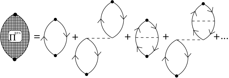
FIG. 4.: Diagrammatic representation of the perturbative expansion for the polarization propagator in random phase approximation.

We have already noted at the beginning of Section II that, while for the two-body Green’s function $G^{\text{ph}}$ one can introduce an integral equation, this is not possible, in general, for the polarization propagator. It becomes possible when one approximates the irreducible vertex function $\Gamma^{13}$ with the direct matrix elements of the interaction. In that case, in an infinite system, one gets a simple algebraic equation, whose solution, for the polarization propagators (2) and the interaction (2), is readily found to be

$$\Pi^{\text{ring}}_{\text{X}}(q,\omega)=\frac{\Pi^{(0)}(q,\omega)}{1-\Pi^{(1)\text{d}}_{\text{X}}(q,\omega)\big{/}\Pi^{(0)}(q,\omega)},$$ (62)

where $\Pi^{(1)\text{d}}_{\text{X}}$ represents the first order direct polarization propagator:

$$\Pi^{(1)\text{d}}_{\text{L};I=0(1)}(q,\omega) = \Pi^{(0)}(q,\omega)4V_{0(\tau)}(q)\Pi^{(0)}(q,\omega),$$ (64)

$$\Pi^{(1)\text{d}}_{\text{T};I=0(1)}(q,\omega) = \Pi^{(0)}(q,\omega)4[V_{\sigma(\sigma\tau)}(q)-V_{t(t\tau)}(q)]\Pi^{(0)}(q,\omega).$$ (65)

The effect of the exchange diagrams is often included through an effective zero-range interaction, calculated by taking the limit $q\to 0$ of the first order exchange contribution and rewriting it as an effective first order direct term [30]. Exact calculations, however, show that extrapolating this approximation to finite transferred momenta is not always reliable [6].

A more sophisticated approximation scheme is given by the continued fraction expansion [31, 4, 5, 32]. At infinite order the CF expansion gives the exact result as the summation of the perturbative series, so that it is not easier to calculate: However, when truncated at finite order, it reproduces the standard perturbative series at the same order plus an approximation for each one of the infinite number of higher order contributions. The trouble here is that there is no general method to predict the convergence of the CF expansion, the only reliable test being a direct comparison of the results at successive orders.

On the other hand, we should note that for zero-range forces the first order CF expansion already gives the exact (albeit trivial) result, making one hope that the short-range nature of the nuclear interactions allows for a fast convergence. Indeed, all available calculations have been performed truncating the CF expansion at first order [4, 5, 24, 25, 13, 20]. Here, as anticipated, we shall test the convergence up to second order.

The CF formalism for the polarization propagator is developed in Ref. [4] for the case of Tamm-Dancoff correlations and extended in Ref. [5] to the full RPA. Instead of following the rather involved formal derivation given there, we shall briefly sketch a sort of heuristic derivation of the CF expansion (which is, of course, only possible “a posteriori”, once the meaning of the CF series has been understood).

Let us assume that we want to build a CF-like expansion for the polarization propagator, according to the pattern

$$\Pi^{\text{RPA}}=\frac{\Pi^{(0)}}{\displaystyle 1-A-\frac{B}{\displaystyle 1-C-\frac{D}{\displaystyle 1-...}}}.$$ (66)

We have said that the CF approach at $n$-th order reproduces the perturbative series at the same order and then it approximates higher orders. Thus, if we want to approximate at first order in CF the exact RPA propagator (for sake of illustration we drop spin-isospin indices),

$$\Pi^{\text{RPA}}=\sum_{n=0}^{\infty}\Pi^{(n)},$$ (67)

we can rather naturally write

$$\Pi^{(n)}\cong\Pi^{(0)}\left[\frac{\Pi^{(1)}}{\Pi^{(0)}}\right]^{n},$$ (68)

where $\Pi^{(1)}\equiv\Pi^{(0)}4V\Pi^{(0)}+\Pi^{(1)\text{ex}}$ is the sum of the direct and exchange first order terms, — since this is the correct expression for the direct terms. With this approximation the summation is trivial, yielding

$$\Pi^{\text{RPA}}_{\text{CF1}}=\frac{\Pi^{(0)}}{1-\Pi^{(1)}/\Pi^{(0)}}=\frac{\Pi^{(0)}}{1-4V\Pi^{(0)}-\Pi^{(1)\text{ex}}/\Pi^{(0)}}.$$ (69)

We could then add in the denominator of the expression above the exact second order term, $\Pi^{(2)}$, having care of subtracting the approximation to it provided by the first order CF expansion, $[\Pi^{(1)}]^{2}/\Pi^{(0)}$. Then, we would get

$$\Pi^{\text{RPA}}_{\text{CF2}} = \frac{\Pi^{(0)}}{1-\Pi^{(1)}/\Pi^{(0)}-\{\Pi^{(2)}/\Pi^{(0)}-[\Pi^{(1)}/\Pi^{(0)}]^{2}\}}$$ (70)

$$= \frac{\Pi^{(0)}}{1-4V\Pi^{(0)}-\Pi^{(1)\text{ex}}/\Pi^{(0)}-\{\Pi^{(2)\text{ex}}/\Pi^{(0)}-[\Pi^{(1)\text{ex}}/\Pi^{(0)}]^{2}\}}.$$ (71)

From Eq. (71) it is easy to check that the third order term is approximated as $\Pi^{(3)}\cong\Pi^{(1)}\{2\Pi^{(2)}/\Pi^{(0)}-[\Pi^{(1)}/\Pi^{(0)}]^{2}\}$. Then, going ahead in a CF-style expansion we would guess for the exact RPA propagator the following expression:

$$\Pi^{\text{RPA}}=\frac{\Pi^{(0)}}{\displaystyle 1-\Pi^{(1)}/\Pi^{(0)}-\frac{\Pi^{(2)\text{ex}}/\Pi^{(0)}-[\Pi^{(1)\text{ex}}/\Pi^{(0)}]^{2}}{\displaystyle 1-\frac{\Pi^{(3)\text{ex}}/\Pi^{(0)}+[\Pi^{(1)\text{ex}}/\Pi^{(0)}]^{3}-2[\Pi^{(1)\text{ex}}/\Pi^{(0)}][\Pi^{(2)\text{ex}}/\Pi^{(0)}]}{\displaystyle\Pi^{(2)\text{ex}}/\Pi^{(0)}-[\Pi^{(1)\text{ex}}/\Pi^{(0)}]^{2}}-...}}.$$ (72)

This is exactly the expression one would get from the formalism of Refs. [4, 5] if one had the patience to work out the expansion up to third order. Note that we did not assume any specific scheme (either Tamm-Dancoff or RPA) in this heuristic derivation.

Thus, following (62) we can write

$$\Pi^{\text{RPA}}_{\text{X}}=\frac{\Pi^{(0)}}{\displaystyle 1-\Pi^{(1)\text{d}}_{\text{X}}\big{/}\Pi^{(0)}-\Pi^{(1)\text{ex}}_{\text{X}}\big{/}\Pi^{(0)}-\frac{\Pi^{(2)\text{ex}}_{\text{X}}\big{/}\Pi^{(0)}-\left[\Pi^{(1)\text{ex}}_{\text{X}}\big{/}\Pi^{(0)}\right]^{2}}{\displaystyle 1-...}},$$ (73)

where $\Pi^{(1)\text{d}}_{\text{X}}$ has been defined in (62). Then, truncation at $n$-th order requires the calculation of the exchange contributions up to that order.

From (2) we can write

$$\Pi^{(n)\text{ex}}_{\text{L};I}(q,\omega) = \text{tr}[\hat{O}^{I}_{\text{L}}\hat{\Pi}^{(n)\text{ex}}(q,\omega)\hat{O}^{I}_{\text{L}}]=\sum_{\alpha_{i}}C^{\alpha_{1}...\alpha_{n}}_{\text{L};I}\Pi^{(n)\text{ex}}_{\alpha_{1}...\alpha_{n}}(q,\omega),$$ (75)

$$\Pi^{(n)\text{ex}}_{\text{T};I}(q,\omega) = \sum_{ij}\Lambda_{ji}\text{tr}[\hat{O}^{I}_{\text{T};i}\hat{\Pi}^{(n)\text{ex}}(q,\omega)\hat{O}^{I}_{\text{T};j}]=\sum_{\alpha_{i}}C^{\alpha_{1}...\alpha_{n}}_{\text{T};I}\Pi^{(n)\text{ex}}_{\alpha_{1}...\alpha_{n}}(q,\omega),$$ (76)

where the indices $\alpha_{i}$ run over all the spin-isospin channels and the spin-isospin factors are condensed in the coefficients $C^{\alpha_{1}...\alpha_{n}}_{\text{X}}\equiv C^{(\alpha_{1})}_{\text{X}}C^{(\alpha_{2})}_{\text{X}}...C^{(\alpha_{n})}_{\text{X}}$ (see Table I).

$\phantom{\Big{|}}X$	$C^{0}_{X}$	$C^{\tau}_{X}$	$C^{\sigma}_{X}$	$C^{\sigma\tau}_{X}$	$C^{t}_{X}$	$C^{t\tau}_{X}$
$L;I=0$	1	3	3	9	0	0
$L;I=1$	1	-1	3	-3	0	0
$T;I=0$	1	3	-1	-3	-1	-3
$T;I=1$	1	-1	-1	1	-1	1

TABLE I.: The spin-isospin coefficients $C^{\alpha}_{X}$ (see text), in the longitudinal and transverse isoscalar and isovector channels, for the interaction (2).

We have introduced the “elementary” exchange contribution $\Pi^{(n)\text{ex}}_{\alpha_{1}...\alpha_{n}}$ containing $n$ interaction lines $V_{\alpha_{1}}$…$V_{\alpha_{n}}$, namely

$$\Pi^{(n)\text{ex}}_{\alpha_{1}...\alpha_{n}}(q,\omega) = -i^{n+1}\int\frac{d^{4}K_{1}}{(2\pi)^{4}}\cdot\cdot\cdot\frac{d^{4}K_{n+1}}{(2\pi)^{4}}G^{(0)}(K_{1})G^{(0)}(K_{1}+Q)V_{\alpha_{1}}(\mathchoice{{\hbox{\boldmath$\displaystyle k$}}}{{\hbox{\boldmath$\textstyle k$}}}{{\hbox{\boldmath$\scriptstyle k$}}}{{\hbox{\boldmath$\scriptscriptstyle k$}}}_{1}-\mathchoice{{\hbox{\boldmath$\displaystyle k$}}}{{\hbox{\boldmath$\textstyle k$}}}{{\hbox{\boldmath$\scriptstyle k$}}}{{\hbox{\boldmath$\scriptscriptstyle k$}}}_{2})\cdot\cdot\cdot$$ (78)

$$\qquad\cdot\cdot\cdot V_{\alpha_{n}}(\mathchoice{{\hbox{\boldmath$\displaystyle k$}}}{{\hbox{\boldmath$\textstyle k$}}}{{\hbox{\boldmath$\scriptstyle k$}}}{{\hbox{\boldmath$\scriptscriptstyle k$}}}_{n}-\mathchoice{{\hbox{\boldmath$\displaystyle k$}}}{{\hbox{\boldmath$\textstyle k$}}}{{\hbox{\boldmath$\scriptstyle k$}}}{{\hbox{\boldmath$\scriptscriptstyle k$}}}_{n+1})G^{(0)}(K_{n+1})G^{(0)}(K_{n+1}+Q)$$

$$= (-1)^{n}\int\frac{d\mathchoice{{\hbox{\boldmath$\displaystyle k$}}}{{\hbox{\boldmath$\textstyle k$}}}{{\hbox{\boldmath$\scriptstyle k$}}}{{\hbox{\boldmath$\scriptscriptstyle k$}}}_{1}}{(2\pi)^{3}}\cdot\cdot\cdot\frac{d\mathchoice{{\hbox{\boldmath$\displaystyle k$}}}{{\hbox{\boldmath$\textstyle k$}}}{{\hbox{\boldmath$\scriptstyle k$}}}{{\hbox{\boldmath$\scriptscriptstyle k$}}}_{n+1}}{(2\pi)^{3}}G^{(0)}_{\text{ph}}(\mathchoice{{\hbox{\boldmath$\displaystyle k$}}}{{\hbox{\boldmath$\textstyle k$}}}{{\hbox{\boldmath$\scriptstyle k$}}}{{\hbox{\boldmath$\scriptscriptstyle k$}}}_{1},\mathchoice{{\hbox{\boldmath$\displaystyle q$}}}{{\hbox{\boldmath$\textstyle q$}}}{{\hbox{\boldmath$\scriptstyle q$}}}{{\hbox{\boldmath$\scriptscriptstyle q$}}};\omega)V_{\alpha_{1}}(\mathchoice{{\hbox{\boldmath$\displaystyle k$}}}{{\hbox{\boldmath$\textstyle k$}}}{{\hbox{\boldmath$\scriptstyle k$}}}{{\hbox{\boldmath$\scriptscriptstyle k$}}}_{1}-\mathchoice{{\hbox{\boldmath$\displaystyle k$}}}{{\hbox{\boldmath$\textstyle k$}}}{{\hbox{\boldmath$\scriptstyle k$}}}{{\hbox{\boldmath$\scriptscriptstyle k$}}}_{2})\cdot\cdot\cdot$$ (80)

$$\qquad\cdot\cdot\cdot V_{\alpha_{n}}(\mathchoice{{\hbox{\boldmath$\displaystyle k$}}}{{\hbox{\boldmath$\textstyle k$}}}{{\hbox{\boldmath$\scriptstyle k$}}}{{\hbox{\boldmath$\scriptscriptstyle k$}}}_{n}-\mathchoice{{\hbox{\boldmath$\displaystyle k$}}}{{\hbox{\boldmath$\textstyle k$}}}{{\hbox{\boldmath$\scriptstyle k$}}}{{\hbox{\boldmath$\scriptscriptstyle k$}}}_{n+1})G^{(0)}_{\text{ph}}(\mathchoice{{\hbox{\boldmath$\displaystyle k$}}}{{\hbox{\boldmath$\textstyle k$}}}{{\hbox{\boldmath$\scriptstyle k$}}}{{\hbox{\boldmath$\scriptscriptstyle k$}}}_{n+1},\mathchoice{{\hbox{\boldmath$\displaystyle q$}}}{{\hbox{\boldmath$\textstyle q$}}}{{\hbox{\boldmath$\scriptstyle q$}}}{{\hbox{\boldmath$\scriptscriptstyle q$}}};\omega).$$

With the definition of $G^{(0)}_{\text{ph}}$ given in (35) one can, — by a suitable change of integration variables, — eliminate all the $\theta$-functions that contain angular integration variables, leaving a multiple integral with the following general structure:

$$\Pi^{(n)\text{ex}}_{\alpha_{1}...\alpha_{n}}(q,\omega)=(-1)^{n}\int\frac{d\mathchoice{{\hbox{\boldmath$\displaystyle k$}}}{{\hbox{\boldmath$\textstyle k$}}}{{\hbox{\boldmath$\scriptstyle k$}}}{{\hbox{\boldmath$\scriptscriptstyle k$}}}_{1}}{(2\pi)^{3}}\theta(k_{F}-k_{1})\cdot\cdot\cdot\frac{d\mathchoice{{\hbox{\boldmath$\displaystyle k$}}}{{\hbox{\boldmath$\textstyle k$}}}{{\hbox{\boldmath$\scriptstyle k$}}}{{\hbox{\boldmath$\scriptscriptstyle k$}}}_{n+1}}{(2\pi)^{3}}\theta(k_{F}-k_{n+1})$$ (81)

$$\quad\times\Big{[}\frac{1}{\omega-\epsilon_{\mathchoice{{\hbox{\boldmath$\displaystyle k$}}}{{\hbox{\boldmath$\textstyle k$}}}{{\hbox{\boldmath$\scriptstyle k$}}}{{\hbox{\boldmath$\scriptscriptstyle k$}}}_{1}+\mathchoice{{\hbox{\boldmath$\displaystyle q$}}}{{\hbox{\boldmath$\textstyle q$}}}{{\hbox{\boldmath$\scriptstyle q$}}}{{\hbox{\boldmath$\scriptscriptstyle q$}}}}+\epsilon_{\mathchoice{{\hbox{\boldmath$\displaystyle k$}}}{{\hbox{\boldmath$\textstyle k$}}}{{\hbox{\boldmath$\scriptstyle k$}}}{{\hbox{\boldmath$\scriptscriptstyle k$}}}_{1}}+i\eta_{\omega}}V_{\alpha_{1}}(\mathchoice{{\hbox{\boldmath$\displaystyle k$}}}{{\hbox{\boldmath$\textstyle k$}}}{{\hbox{\boldmath$\scriptstyle k$}}}{{\hbox{\boldmath$\scriptscriptstyle k$}}}_{1}-\mathchoice{{\hbox{\boldmath$\displaystyle k$}}}{{\hbox{\boldmath$\textstyle k$}}}{{\hbox{\boldmath$\scriptstyle k$}}}{{\hbox{\boldmath$\scriptscriptstyle k$}}}_{2})\cdot\cdot\cdot V_{\alpha_{n}}(\mathchoice{{\hbox{\boldmath$\displaystyle k$}}}{{\hbox{\boldmath$\textstyle k$}}}{{\hbox{\boldmath$\scriptstyle k$}}}{{\hbox{\boldmath$\scriptscriptstyle k$}}}_{n}-\mathchoice{{\hbox{\boldmath$\displaystyle k$}}}{{\hbox{\boldmath$\textstyle k$}}}{{\hbox{\boldmath$\scriptstyle k$}}}{{\hbox{\boldmath$\scriptscriptstyle k$}}}_{n+1})\frac{1}{\omega-\epsilon_{\mathchoice{{\hbox{\boldmath$\displaystyle k$}}}{{\hbox{\boldmath$\textstyle k$}}}{{\hbox{\boldmath$\scriptstyle k$}}}{{\hbox{\boldmath$\scriptscriptstyle k$}}}_{n+1}+\mathchoice{{\hbox{\boldmath$\displaystyle q$}}}{{\hbox{\boldmath$\textstyle q$}}}{{\hbox{\boldmath$\scriptstyle q$}}}{{\hbox{\boldmath$\scriptscriptstyle q$}}}}+\epsilon_{\mathchoice{{\hbox{\boldmath$\displaystyle k$}}}{{\hbox{\boldmath$\textstyle k$}}}{{\hbox{\boldmath$\scriptstyle k$}}}{{\hbox{\boldmath$\scriptscriptstyle k$}}}_{n+1}}+i\eta_{\omega}}$$ (82)

$$\quad\quad+\sum(\omega\to-\omega)\Big{]}.$$ (83)

In (83), $\sum(\omega\to-\omega)$ stands for the sum of all the terms generated according to the following rules:

• take all the terms generated by substituting, in the second line of (83), in one energy denominator $\omega\to-\omega$; then, by doing the same substitution in two energy denominators; and so on up to making the replacement $\omega\to-\omega$ in all the $n+1$ denominators;

• every time $(\omega-\epsilon_{\mathchoice{{\hbox{\boldmath$\displaystyle k$}}}{{\hbox{\boldmath$\textstyle k$}}}{{\hbox{\boldmath$\scriptstyle k$}}}{{\hbox{\boldmath$\scriptscriptstyle k$}}}_{i}+\mathchoice{{\hbox{\boldmath$\displaystyle q$}}}{{\hbox{\boldmath$\textstyle q$}}}{{\hbox{\boldmath$\scriptstyle q$}}}{{\hbox{\boldmath$\scriptscriptstyle q$}}}}+\epsilon_{\mathchoice{{\hbox{\boldmath$\displaystyle k$}}}{{\hbox{\boldmath$\textstyle k$}}}{{\hbox{\boldmath$\scriptstyle k$}}}{{\hbox{\boldmath$\scriptscriptstyle k$}}}_{i}}+i\eta_{\omega})^{-1}$ is replaced with $(-\omega-\epsilon_{\mathchoice{{\hbox{\boldmath$\displaystyle k$}}}{{\hbox{\boldmath$\textstyle k$}}}{{\hbox{\boldmath$\scriptstyle k$}}}{{\hbox{\boldmath$\scriptscriptstyle k$}}}_{i}+\mathchoice{{\hbox{\boldmath$\displaystyle q$}}}{{\hbox{\boldmath$\textstyle q$}}}{{\hbox{\boldmath$\scriptstyle q$}}}{{\hbox{\boldmath$\scriptscriptstyle q$}}}}+\epsilon_{\mathchoice{{\hbox{\boldmath$\displaystyle k$}}}{{\hbox{\boldmath$\textstyle k$}}}{{\hbox{\boldmath$\scriptstyle k$}}}{{\hbox{\boldmath$\scriptscriptstyle k$}}}_{i}}-i\eta_{\omega})^{-1}$, then replace $\mathchoice{{\hbox{\boldmath$\displaystyle k$}}}{{\hbox{\boldmath$\textstyle k$}}}{{\hbox{\boldmath$\scriptstyle k$}}}{{\hbox{\boldmath$\scriptscriptstyle k$}}}_{i}$ with $-\mathchoice{{\hbox{\boldmath$\displaystyle k$}}}{{\hbox{\boldmath$\textstyle k$}}}{{\hbox{\boldmath$\scriptstyle k$}}}{{\hbox{\boldmath$\scriptscriptstyle k$}}}_{i}-\mathchoice{{\hbox{\boldmath$\displaystyle q$}}}{{\hbox{\boldmath$\textstyle q$}}}{{\hbox{\boldmath$\scriptstyle q$}}}{{\hbox{\boldmath$\scriptscriptstyle q$}}}$ in the potentials.

The number of integrations can be reduced by noticing that the azimuthal angles are contained only in the potential functions $V_{\alpha_{i}}$. For typical nuclear physics potentials this integration can be done analytically, so that it is convenient to introduce a new function representing the azimuthal integral of the potential. To this end, let us define new variables:

$$|\mathchoice{{\hbox{\boldmath$\displaystyle k$}}}{{\hbox{\boldmath$\textstyle k$}}}{{\hbox{\boldmath$\scriptstyle k$}}}{{\hbox{\boldmath$\scriptscriptstyle k$}}}-\mathchoice{{\hbox{\boldmath$\displaystyle k$}}}{{\hbox{\boldmath$\textstyle k$}}}{{\hbox{\boldmath$\scriptstyle k$}}}{{\hbox{\boldmath$\scriptscriptstyle k$}}}^{\prime}| = \sqrt{k^{2}+{k^{\prime}}^{2}-2kk^{\prime}[\cos\theta\,\cos\theta^{\prime}+\sin\theta\,\sin\theta^{\prime}\,\cos(\varphi-\varphi^{\prime})]}$$ (84)

$$= \sqrt{k^{2}+{k^{\prime}}^{2}-2[yy^{\prime}+\sqrt{k^{2}-y^{2}}\sqrt{{k^{\prime}}^{2}-{y^{\prime}}^{2}}\cos(\varphi-\varphi^{\prime})]}$$ (85)

$$= \sqrt{x+x^{\prime}-2\sqrt{x}\sqrt{x^{\prime}}\cos(\varphi-\varphi^{\prime})+(y-y^{\prime})^{2}},$$ (86)

where $y\equiv k\,\cos\theta$ and $x\equiv k^{2}-y^{2}$. Then, we can introduce

$$W_{\alpha}(x,y;x^{\prime},y^{\prime})=\int_{0}^{2\pi}\frac{d\varphi}{2\pi}V_{\alpha}(\mathchoice{{\hbox{\boldmath$\displaystyle k$}}}{{\hbox{\boldmath$\textstyle k$}}}{{\hbox{\boldmath$\scriptstyle k$}}}{{\hbox{\boldmath$\scriptscriptstyle k$}}}-\mathchoice{{\hbox{\boldmath$\displaystyle k$}}}{{\hbox{\boldmath$\textstyle k$}}}{{\hbox{\boldmath$\scriptstyle k$}}}{{\hbox{\boldmath$\scriptscriptstyle k$}}}^{\prime})=W_{\alpha}(x^{\prime},y^{\prime};x,y)$$ (87)

and rewrite (83) as

$$\Pi^{(n)\text{ex}}_{\alpha_{1}...\alpha_{n}}(q,\omega) = (-1)^{n}\left(\frac{m_{N}}{q}\right)^{n+1}\left(\frac{k_{F}}{2\pi}\right)^{2n+2}\int_{-1}^{1}dy_{1}\frac{1}{2}\int_{0}^{1-y_{1}^{2}}dx_{1}\cdot\cdot\cdot\int_{-1}^{1}dy_{n+1}\frac{1}{2}\int_{0}^{1-y_{n+1}^{2}}dx_{n+1}$$ (90)

$$\times\frac{1}{\psi-y_{1}+i\eta_{\omega}}W_{\alpha_{1}}(x_{1},y_{1};x_{2},y_{2})\cdot\cdot\cdot W_{\alpha_{n}}(x_{n},y_{n};x_{n+1},y_{n+1})\frac{1}{\psi-y_{n+1}+i\eta_{\omega}}$$

$$+\sum(\omega\to-\omega).$$

For $n=1$ one has

$$\Pi^{(1)\text{ex}}_{\alpha}(q,\omega) = -\left(\frac{m_{N}}{q}\right)^{2}\frac{k_{F}^{4}}{(2\pi)^{4}}\int_{-1}^{1}dy\frac{1}{2}\int_{0}^{1-y^{2}}dx\int_{-1}^{1}dy^{\prime}\frac{1}{2}\int_{0}^{1-{y^{\prime}}^{2}}dx^{\prime}$$ (93)

$$\times\frac{1}{\psi-y+i\eta_{\omega}}W_{\alpha}(x,y;x^{\prime},y^{\prime})\frac{1}{\psi-y^{\prime}+i\eta_{\omega}}$$

$$+\sum(\omega\to-\omega)$$

$$= -\left(\frac{m_{N}}{q}\right)^{2}\frac{k_{F}^{4}}{(2\pi)^{4}}\left[{\cal Q}_{\alpha}^{(1)}(0,\psi)-{\cal Q}_{\alpha}^{(1)}(\bar{q},\psi)+{\cal Q}_{\alpha}^{(1)}(0,\psi+\bar{q})-{\cal Q}_{\alpha}^{(1)}(-\bar{q},\psi+\bar{q})\right],$$ (94)

where

$${\cal Q}_{\alpha}^{(1)}(\bar{q},\psi)=2\int_{-1}^{1}dy\frac{1}{\psi-y+i\eta_{\omega}}\int_{-1}^{1}dy^{\prime}\,{W_{\alpha}}^{\prime\prime}(y,y^{\prime};\bar{q})\frac{1}{y-y^{\prime}+\bar{q}}$$ (96)

and

$$W^{\prime\prime}_{\alpha}(y,y^{\prime};\bar{q})=\frac{1}{2}\int_{0}^{1-y^{2}}dx\,\frac{1}{2}\int_{0}^{1-{y^{\prime}}^{2}}dx^{\prime}\,W_{\alpha}(x,y+\bar{q};x^{\prime},y^{\prime}).$$ (97)

Note that in getting to Eq. (96) use has been made of the Poincaré–Bertrand theorem [33]. For the potential (* ‣ II) $W^{\prime\prime}_{\alpha}$ can be calculated analytically (see Appendix B), so that the calculation of the first order exchange contribution to the polarization propagator is reduced to the numerical evaluation of two-dimensional integrals, — for the real part, — and of one-dimensional integrals, — for the imaginary part.

For $n=2$ one has

$$\Pi^{(2)\text{ex}}_{\alpha\alpha^{\prime}}(q,\omega)=\left(\frac{m_{N}}{q}\right)^{3}\frac{k_{F}^{6}}{(2\pi)^{6}}\int_{-1}^{1}dy_{1}\frac{1}{2}\int_{0}^{1-y_{1}^{2}}dx_{1}\int_{-1}^{1}dy_{2}\frac{1}{2}\int_{0}^{1-y_{2}^{2}}dx_{2}\int_{-1}^{1}dy_{3}\frac{1}{2}\int_{0}^{1-y_{3}^{2}}dx_{3}$$ (98)

$$\phantom{\Pi^{(2)\text{ex}}_{\alpha\alpha^{\prime}}(q,\omega)=}\times\frac{1}{\psi-y_{1}+i\eta_{\omega}}W_{\alpha}(x_{1},y_{1};x_{2},y_{2})\frac{1}{\psi-y_{2}+i\eta_{\omega}}W_{\alpha}(x_{2},y_{2};x_{3},y_{3})\frac{1}{\psi-y_{3}+i\eta_{\omega}}$$ (99)

$$\phantom{\Pi^{(2)\text{ex}}_{\alpha\alpha^{\prime}}(q,\omega)=}+\sum(\omega\to-\omega)$$ (100)

$$\phantom{\Pi^{(2)\text{ex}}_{\alpha\alpha^{\prime}}(q,\omega)}=\left(\frac{m_{N}}{q}\right)^{3}\frac{k_{F}^{6}}{(2\pi)^{6}}\left[{\cal Q}_{\alpha\alpha^{\prime}}^{(2)}(0,0;\psi)-{\cal Q}_{\alpha\alpha^{\prime}}^{(2)}(0,\bar{q};\psi)-{\cal Q}_{\alpha\alpha^{\prime}}^{(2)}(\bar{q},0;\psi)+{\cal Q}_{\alpha\alpha^{\prime}}^{(2)}(\bar{q},\bar{q};\psi)\right.$$ (101)

$$\qquad\left.-{\cal Q}_{\alpha\alpha^{\prime}}^{(2)}(0,0;\psi+\bar{q})+{\cal Q}_{\alpha\alpha^{\prime}}^{(2)}(0,-\bar{q};\psi+\bar{q})+{\cal Q}_{\alpha\alpha^{\prime}}^{(2)}(-\bar{q},0;\psi+\bar{q})-{\cal Q}_{\alpha\alpha^{\prime}}^{(2)}(-\bar{q},-\bar{q};\psi+\bar{q})\right],$$ (102)

(103)

where

$${\cal Q}_{\alpha\alpha^{\prime}}^{(2)}(\bar{q}_{1},\bar{q}_{2};\psi)=\int_{-1}^{1}dy\frac{1}{2}\int_{0}^{1-y^{2}}dx\,{\cal G}_{\alpha}(x,y+\bar{q}_{1};\psi+\bar{q}_{1})\frac{1}{\psi-y+i\eta_{\omega}}{\cal G}_{\alpha^{\prime}}(x,y+\bar{q}_{2};\psi+\bar{q}_{2})$$ (104)

and

$${\cal G}_{\alpha}(x,y;\psi) = \int_{-1}^{1}dy^{\prime}\frac{1}{\psi-y^{\prime}+i\eta_{\omega}}W^{\prime}_{\alpha}(x,y;y^{\prime}),$$ (106)

$$W^{\prime}_{\alpha}(x,y;y^{\prime}) = \frac{1}{2}\int_{0}^{1-{y^{\prime}}^{2}}dx^{\prime}\,W_{\alpha}(x,y;x^{\prime},y^{\prime}).$$ (107)

For the potential (* ‣ II) $W^{\prime}_{\alpha}$ can be calculated analytically (see Appendix B) and one is left with the numerical integration of (104) and (106), so that the calculation of the second order exchange contribution to the polarization propagator is effectively reduced to the numerical evaluation of at most three-dimensional integrals.

Going to higher orders implies a numerical two-dimensional integration for each supplemental interaction line, since, for a potential of the form (* ‣ II), only the azimuthal integration can be performed analytically for the interaction lines that are not close to the external vertices.

The Hartree-Fock dressing of the nucleon propagators can again be done as explained in Subsection II C, with the replacements $\psi\to\psi^{*}$ and $m_{N}\to m_{N}^{*}$, where $\psi^{*}$ and $m_{N}^{*}$ have been defined in (51) and (56), multiplying by the correct power of the normalization factor $1+\omega/m_{N}+\Delta^{(1)}/m_{N}$ when the relativistic kinematics is employed (see Eqs. (3) and (60).

III Results

First of all we have to choose the Fermi momentum. Of course, one could easily perform a local density calculation to achieve a better description of finite nuclei: Here, for sake of illustration, we prefer to use the pure Fermi gas. The choice of $k_{F}$ can be done in several ways: We shall choose an average value according to the formula

$$\bar{k}_{F}=\frac{1}{A}\int d\mathchoice{{\hbox{\boldmath$\displaystyle r$}}}{{\hbox{\boldmath$\textstyle r$}}}{{\hbox{\boldmath$\scriptstyle r$}}}{{\hbox{\boldmath$\scriptscriptstyle r$}}}k_{F}(r)\rho(r),$$ (108)

where $\rho(r)$ is the empirical Fermi density distribution normalized to the number of nucleons and $k_{F}(r)=[(3\pi/2)\rho(r)]^{1/3}$. For ¹²C one gets $\bar{k}_{F}\approx 195$ MeV/c and this is the value used in the calculations that follow.

FIG. 5.: Fermi gas longitudinal responses for $k_{F}=195$ MeV/c at $q=300$ MeV/c, with a spin-spin one-boson-exchange interaction, for various values of the coupling constant and of the boson mass: Free response (dot), RPA with the first order CF expansion (dash) and RPA with the second order CF expansion (solid). Note that in the left and middle panels the dashed and solid lines are not distinguishable. The kinematics is non-relativistic.

FIG. 6.: Modulus of the longitudinal polarization propagator for $k_{F}=195$ MeV/c at $q=300$ MeV/c, with a spin-spin one-boson-exchange interaction, for various values of the coupling constant and of the boson mass: First order, $\Pi^{\text{(1)}}$ (dot); exact second order, $\Pi^{\text{(2)}}$ (dash); CF approximation to the second order, $\Pi^{\text{(2)appr}}={\Pi^{\text{(1)}}}^{2}/\Pi^{\text{(0)}}$ (solid).

Let us start by testing the convergence of the CF expansion. For this purpose, we compare in Fig. 6 the longitudinal RPA responses at first and second order in the CF expansion using a model one-boson-exchange interaction, $V_{\sigma}(k)=\mathchoice{{\hbox{\boldmath$\displaystyle\sigma$}}}{{\hbox{\boldmath$\textstyle\sigma$}}}{{\hbox{\boldmath$\scriptstyle\sigma$}}}{{\hbox{\boldmath$\scriptscriptstyle\sigma$}}}_{1}\cdot\mathchoice{{\hbox{\boldmath$\displaystyle\sigma$}}}{{\hbox{\boldmath$\textstyle\sigma$}}}{{\hbox{\boldmath$\scriptstyle\sigma$}}}{{\hbox{\boldmath$\scriptscriptstyle\sigma$}}}_{2}g[m^{2}/(m^{2}+k^{2})]$ (the spin operators having the purpose of killing the direct (ring) contribution). For values of the coupling constant $g$ and of the boson mass $m$ typical of realistic nucleon-nucleon potentials one finds that the first and second order results match at the level of a few per cent (in the left and middle panels of Fig. 6, the solid and dashed curved are actually indistinguishable). One has to go to very low boson masses (a few MeV) and, consequently, to very high values of $g$ in order to find some discrepancies. To understand better these results, we display in Fig. 6 the modulus of the polarization propagator at first order, $\Pi^{(1)}$ (dot), at second order, $\Pi^{(2)}$ (dash) and the approximation to $\Pi^{(2)}$ generated by the first order CF expansion (see Section II D), $\Pi^{(2)\text{appr}}\equiv{\Pi^{(1)}}^{2}/\Pi^{(0)}$ (solid). From inspection of the curves, it is clear that the first important element to guarantee a good convergence is the range of the interaction: Indeed, for $m=800$ MeV (short-range) $\Pi^{(2)}$ and $\Pi^{(2)\text{appr}}$ practically coincide independently of the strength of the interaction. This, of course, should be expected, since for zero-range interactions the first order CF expansion gives the exact result. For masses of the order of the pion mass one starts finding discrepancies between $\Pi^{(2)}$ and $\Pi^{(2)\text{appr}}$: However, for realistic values of the interaction strength the second order contribution turns out to be one order of magnitude smaller than the first order one, thus making these discrepancies having no effect on the full response functions (Fig. 6).

To understand these results it may be useful to compare the strength of the interactions employed here to the one of one-pion-exchange, $g_{\pi}m_{\pi}^{2}\equiv f_{\pi}^{2}/3\cong 0.33$ (in natural units). With the same units, the cases with $m=100$ MeV correspond to $g\,m^{2}=0.26$ and 0.65; those with $m=800$ MeV to $g\,m^{2}=16.7$ and 41.7; for $m=1$ and 10 MeV one has $g\,m^{2}=1.3$ and 0.65, respectively.

To summarize, from the left and middle panels of Fig. 6 one can understand that the validity of the CF expansion originates out of the interplay between range and strength of the interaction: For short-range potentials, — where the conventional perturbative expansion may not converge, — the CF technique gives a good approximation of the propagators at all orders; for long-range (on the nuclear scale) forces, the CF approximation is less accurate, but the relative weakness of the interaction already guarantees the convergence of the conventional perturbative expansion. One has to go to unreasonably low masses to find a situation where the interaction range is very long and $\Pi^{(1)}$ and $\Pi^{(2)}$ are of the same order (right panels in Fig. 6).

We can thus conclude that accurate calculations of nuclear response functions in the antisymmetrized RPA can be performed at first order in the CF expansion. The same conclusion is supported also by calculations with a realistic effective interaction, — such as the $G$-matrix parameterization discussed below, — and including HF and relativistic kinematical effects.

Finally, it is interesting and important to test the validity of the ring approximation, — where exchange diagrams are not included, — since this approximation has been widely used in the literature because of its simplicity. In this scheme, the effect of antisymmetrization is mimicked by adding to the direct interaction matrix elements an effective exchange contribution (see, e. g., Ref. [30]). For details see also Ref. [34], where a prescription, suitable for the quasifree region, to determine the effective exchange momentum has been given.

FIG. 7.: Fermi gas responses for $k_{F}=195$ MeV/c at $q=500$ MeV/c, with the $G$-matrix parameterization discussed in the text: Free response (dot), ring approximation (dash) and RPA (solid). The kinematics is relativistic.

In Fig. 7, then, we display the ring and RPA responses of ¹²C at $q=500$ MeV/c, using the $G$-matrix parameterization. It is apparent that the only channel where the ring approximation works reasonably well is the spin-isovector one, — which, incidentally, is the dominant one in ($e$,$e^{\prime}$) magnetic scattering; it is less accurate in all the other channels, particularly in the scalar-isoscalar one. The same considerations apply also when HF correlations are included in the ring and RPA responses. Note that these results confirm those of Ref. [6], where a comparison of ring and RPA calculations had been done using a numerically rather involved finite nucleus formalism. Also in that calculation the $G$-matrix of Ref. [22] had been employed.

IV Concluding remarks

In this paper we have illustrated a fast and compact scheme for the calculation of the fully antisymmetrized RPA response functions in nuclear matter, based on the CF expansion. The fast convergence of the CF series for typical nucleon-nucleon potentials has been demonstrated, thus making this technique a very convenient tool for the exact resummation of the RPA diagrams. On the other hand the poor performance in most spin-isospin channels of the ring approximation, — where the exchange diagrams are not included, — has been confirmed. Accurate approximations for the inclusion of the relativistic kinematics and of HF effects have also been discussed and tested.

Although other classes of contributions are also necessary to make contact with the electron scattering phenomenology, — such as meson exchange currents and higher order ph configurations, — we believe that the methods discussed in this paper provide a good, — because of the accuracy, — and convenient, — because of the simplicity, — starting point. As mentioned in the Introduction, it would also be interesting a comparison, under the same approximation schemes, with other approaches, such as those based on the relativistic models of nuclear structure.

A Tensor interaction in the exchange diagrams

The $n$-th order exchange polarization propagator in presence of tensor interactions has an expression slightly more complicated than (90), because the tensor operators do not allow, in general, for a factorization of the azimuthal integrations. A generic diagram with $m$ non-tensor and $n-m$ tensor interaction lines can instead be written as

$$\Pi^{(n)\text{ex}}_{\alpha_{1}...\alpha_{m},\alpha_{m+1}...\alpha_{n}}(q,\omega) = (-1)^{n}\left(\frac{m_{N}}{q}\right)^{n+1}\left(\frac{k_{F}}{2\pi}\right)^{2n+2}$$ (A5)

$$\times\int_{-1}^{1}dy_{1}\frac{1}{2}\int_{0}^{1-y_{1}^{2}}dx_{1}\cdot\cdot\cdot\int_{-1}^{1}dy_{n+1}\frac{1}{2}\int_{0}^{1-y_{n+1}^{2}}dx_{n+1}$$

$$\times\frac{1}{\psi-y_{1}+i\eta_{\omega}}W_{\alpha_{1}}(x_{1},y_{1};x_{2},y_{2})\cdot\cdot\cdot W_{\alpha_{m}}(x_{m},y_{m};x_{m+1},y_{m+1})$$

$$\times W_{\alpha_{m+1}...\alpha_{n}}(x_{m+1},y_{m+1};...;x_{n+1},y_{n+1})\frac{1}{\psi-y_{n+1}+i\eta_{\omega}}$$

$$+\sum(\omega\to-\omega),$$

where $W_{\alpha_{i}}$ has been defined in (87) for the non-tensor channels and

$$W_{\alpha_{m+1}...\alpha_{n}}(x_{m+1},y_{m+1};...;x_{n+1},y_{n+1})=2^{n-m}\sum_{ij}\sum_{l_{1}...l_{n-m}}\Lambda_{ji}\int_{0}^{2\pi}\frac{d\varphi_{m+1}}{2\pi}...\int_{0}^{2\pi}\frac{d\varphi_{n+1}}{2\pi}$$ (A6)

$$\qquad\times V_{\alpha_{m+1}}(\mathchoice{{\hbox{\boldmath$\displaystyle k$}}}{{\hbox{\boldmath$\textstyle k$}}}{{\hbox{\boldmath$\scriptstyle k$}}}{{\hbox{\boldmath$\scriptscriptstyle k$}}}_{m+1}-\mathchoice{{\hbox{\boldmath$\displaystyle k$}}}{{\hbox{\boldmath$\textstyle k$}}}{{\hbox{\boldmath$\scriptstyle k$}}}{{\hbox{\boldmath$\scriptscriptstyle k$}}}_{m+2})S_{il_{1}}(\widehat{\mathchoice{{\hbox{\boldmath$\displaystyle k$}}}{{\hbox{\boldmath$\textstyle k$}}}{{\hbox{\boldmath$\scriptstyle k$}}}{{\hbox{\boldmath$\scriptscriptstyle k$}}}_{m+1}-\mathchoice{{\hbox{\boldmath$\displaystyle k$}}}{{\hbox{\boldmath$\textstyle k$}}}{{\hbox{\boldmath$\scriptstyle k$}}}{{\hbox{\boldmath$\scriptscriptstyle k$}}}_{m+2}})...V_{\alpha_{n}}(\mathchoice{{\hbox{\boldmath$\displaystyle k$}}}{{\hbox{\boldmath$\textstyle k$}}}{{\hbox{\boldmath$\scriptstyle k$}}}{{\hbox{\boldmath$\scriptscriptstyle k$}}}_{n}-\mathchoice{{\hbox{\boldmath$\displaystyle k$}}}{{\hbox{\boldmath$\textstyle k$}}}{{\hbox{\boldmath$\scriptstyle k$}}}{{\hbox{\boldmath$\scriptscriptstyle k$}}}_{n+1})S_{l_{n-m}j}(\widehat{\mathchoice{{\hbox{\boldmath$\displaystyle k$}}}{{\hbox{\boldmath$\textstyle k$}}}{{\hbox{\boldmath$\scriptstyle k$}}}{{\hbox{\boldmath$\scriptscriptstyle k$}}}_{n}-\mathchoice{{\hbox{\boldmath$\displaystyle k$}}}{{\hbox{\boldmath$\textstyle k$}}}{{\hbox{\boldmath$\scriptstyle k$}}}{{\hbox{\boldmath$\scriptscriptstyle k$}}}_{n+1}}).$$ (A7)

In the last expression we have introduced the tensors

$$S_{ij}(\hat{\mathchoice{{\hbox{\boldmath$\displaystyle k$}}}{{\hbox{\boldmath$\textstyle k$}}}{{\hbox{\boldmath$\scriptstyle k$}}}{{\hbox{\boldmath$\scriptscriptstyle k$}}}})=3\hat{\mathchoice{{\hbox{\boldmath$\displaystyle k$}}}{{\hbox{\boldmath$\textstyle k$}}}{{\hbox{\boldmath$\scriptstyle k$}}}{{\hbox{\boldmath$\scriptscriptstyle k$}}}}_{i}\hat{\mathchoice{{\hbox{\boldmath$\displaystyle k$}}}{{\hbox{\boldmath$\textstyle k$}}}{{\hbox{\boldmath$\scriptstyle k$}}}{{\hbox{\boldmath$\scriptscriptstyle k$}}}}j-\delta_{ij},$$ (A8)

such that $\sum_{ij}\sigma_{i}\sigma_{j}S_{ij}(\hat{\mathchoice{{\hbox{\boldmath$\displaystyle k$}}}{{\hbox{\boldmath$\textstyle k$}}}{{\hbox{\boldmath$\scriptstyle k$}}}{{\hbox{\boldmath$\scriptscriptstyle k$}}}})=S_{12}(\hat{\mathchoice{{\hbox{\boldmath$\displaystyle k$}}}{{\hbox{\boldmath$\textstyle k$}}}{{\hbox{\boldmath$\scriptstyle k$}}}{{\hbox{\boldmath$\scriptscriptstyle k$}}}})$.

The first order case is rather simple, since one gets again (LABEL:eq:Pi1ex)–(97) with

$$W_{\alpha}(x,y;x^{\prime},y^{\prime})=\int_{0}^{2\pi}\frac{d\varphi}{2\pi}V_{\alpha}(\mathchoice{{\hbox{\boldmath$\displaystyle k$}}}{{\hbox{\boldmath$\textstyle k$}}}{{\hbox{\boldmath$\scriptstyle k$}}}{{\hbox{\boldmath$\scriptscriptstyle k$}}}-\mathchoice{{\hbox{\boldmath$\displaystyle k$}}}{{\hbox{\boldmath$\textstyle k$}}}{{\hbox{\boldmath$\scriptstyle k$}}}{{\hbox{\boldmath$\scriptscriptstyle k$}}}^{\prime})S_{zz}(\widehat{\mathchoice{{\hbox{\boldmath$\displaystyle k$}}}{{\hbox{\boldmath$\textstyle k$}}}{{\hbox{\boldmath$\scriptstyle k$}}}{{\hbox{\boldmath$\scriptscriptstyle k$}}}-\mathchoice{{\hbox{\boldmath$\displaystyle k$}}}{{\hbox{\boldmath$\textstyle k$}}}{{\hbox{\boldmath$\scriptstyle k$}}}{{\hbox{\boldmath$\scriptscriptstyle k$}}}^{\prime}}).$$ (A9)

At second order, however, one can use Eqs. (103)–(104) only when just one tensor interaction is present.

B First and second order exchange diagrams

We give here the explicit expressions for the first and second order exchange diagrams, based on the potential (2)–(* ‣ II). In (LABEL:eq:Pi1ex) and (96) we have seen that

$$\Pi^{(1)\text{ex}}_{\alpha}(q,\omega)=-\left(\frac{m_{N}}{q}\right)^{2}\frac{k_{F}^{4}}{(2\pi)^{4}}\left[{\cal Q}_{\alpha}^{(1)}(0,\psi)-{\cal Q}_{\alpha}^{(1)}(\bar{q},\psi)+{\cal Q}_{\alpha}^{(1)}(0,\psi+\bar{q})-{\cal Q}_{\alpha}^{(1)}(-\bar{q},\psi+\bar{q})\right],$$ (B1)

where

$${\cal Q}_{\alpha}^{(1)}(\bar{q},\psi)=2\int_{-1}^{1}dy\frac{1}{\psi-y+i\eta_{\omega}}\int_{-1}^{1}dy^{\prime}\,{W_{\alpha}}^{\prime\prime}(y,y^{\prime};\bar{q})\frac{1}{y-y^{\prime}+\bar{q}},$$ (B2)

whereas from (103) and (104) one has

$$\Pi^{(2)\text{ex}}_{\alpha\alpha^{\prime}}(q,\omega)=\left(\frac{m_{N}}{q}\right)^{3}\frac{k_{F}^{6}}{(2\pi)^{6}}\left[{\cal Q}_{\alpha\alpha^{\prime}}^{(2)}(0,0;\psi)-{\cal Q}_{\alpha\alpha^{\prime}}^{(2)}(0,\bar{q};\psi)-{\cal Q}_{\alpha\alpha^{\prime}}^{(2)}(\bar{q},0;\psi)+{\cal Q}_{\alpha\alpha^{\prime}}^{(2)}(\bar{q},\bar{q};\psi)\right.$$ (B3)

$$\qquad\left.-{\cal Q}_{\alpha\alpha^{\prime}}^{(2)}(0,0;\psi+\bar{q})+{\cal Q}_{\alpha\alpha^{\prime}}^{(2)}(0,-\bar{q};\psi+\bar{q})+{\cal Q}_{\alpha\alpha^{\prime}}^{(2)}(-\bar{q},0;\psi+\bar{q})-{\cal Q}_{\alpha\alpha^{\prime}}^{(2)}(-\bar{q},-\bar{q};\psi+\bar{q})\right],$$ (B4)

where

$${\cal Q}_{\alpha\alpha^{\prime}}^{(2)}(\bar{q}_{1},\bar{q}_{2};\psi)=\int_{-1}^{1}dy\frac{1}{2}\int_{0}^{1-y^{2}}dx\,{\cal G}_{\alpha}(x,y+\bar{q}_{1};\psi+\bar{q}_{1})\frac{1}{\psi-y+i\eta_{\omega}}{\cal G}_{\alpha^{\prime}}(x,y+\bar{q}_{2};\psi+\bar{q}_{2})$$ (B6)

and

$${\cal G}_{\alpha}(x,y;\psi)=\int_{-1}^{1}dy^{\prime}\frac{1}{\psi-y^{\prime}+i\eta_{\omega}}W^{\prime}_{\alpha}(x,y;y^{\prime}).$$ (B7)

For a meson-exchange potential the quantities that can be calculated analytically are those given by Eqs. (87), (A9), (107) and (97), namely

$$W_{\alpha}(x,y;x^{\prime},y^{\prime}) = \int_{0}^{2\pi}\frac{d\varphi}{2\pi}V_{\alpha}(\mathchoice{{\hbox{\boldmath$\displaystyle k$}}}{{\hbox{\boldmath$\textstyle k$}}}{{\hbox{\boldmath$\scriptstyle k$}}}{{\hbox{\boldmath$\scriptscriptstyle k$}}}-\mathchoice{{\hbox{\boldmath$\displaystyle k$}}}{{\hbox{\boldmath$\textstyle k$}}}{{\hbox{\boldmath$\scriptstyle k$}}}{{\hbox{\boldmath$\scriptscriptstyle k$}}}^{\prime})\phantom{S_{zz}(\widehat{\mathchoice{{\hbox{\boldmath$\displaystyle k$}}}{{\hbox{\boldmath$\textstyle k$}}}{{\hbox{\boldmath$\scriptstyle k$}}}{{\hbox{\boldmath$\scriptscriptstyle k$}}}-\mathchoice{{\hbox{\boldmath$\displaystyle k$}}}{{\hbox{\boldmath$\textstyle k$}}}{{\hbox{\boldmath$\scriptstyle k$}}}{{\hbox{\boldmath$\scriptscriptstyle k$}}}^{\prime}})}\qquad\text{(non-tensor)}$$ (B9)

$$W_{\alpha}(x,y;x^{\prime},y^{\prime}) = \int_{0}^{2\pi}\frac{d\varphi}{2\pi}V_{\alpha}(\mathchoice{{\hbox{\boldmath$\displaystyle k$}}}{{\hbox{\boldmath$\textstyle k$}}}{{\hbox{\boldmath$\scriptstyle k$}}}{{\hbox{\boldmath$\scriptscriptstyle k$}}}-\mathchoice{{\hbox{\boldmath$\displaystyle k$}}}{{\hbox{\boldmath$\textstyle k$}}}{{\hbox{\boldmath$\scriptstyle k$}}}{{\hbox{\boldmath$\scriptscriptstyle k$}}}^{\prime})S_{zz}(\widehat{\mathchoice{{\hbox{\boldmath$\displaystyle k$}}}{{\hbox{\boldmath$\textstyle k$}}}{{\hbox{\boldmath$\scriptstyle k$}}}{{\hbox{\boldmath$\scriptscriptstyle k$}}}-\mathchoice{{\hbox{\boldmath$\displaystyle k$}}}{{\hbox{\boldmath$\textstyle k$}}}{{\hbox{\boldmath$\scriptstyle k$}}}{{\hbox{\boldmath$\scriptscriptstyle k$}}}^{\prime}})\qquad\text{(tensor)}$$ (B10)

and

$$W^{\prime}_{\alpha}(x,y;y^{\prime}) = \frac{1}{2}\int_{0}^{1-{y^{\prime}}^{2}}dx^{\prime}\,W_{\alpha}(x,y;x^{\prime},y^{\prime})$$ (B11)

$$W^{\prime\prime}_{\alpha}(y,y^{\prime};\bar{q}) = \frac{1}{2}\int_{0}^{1-y^{2}}dx\,\frac{1}{2}\int_{0}^{1-{y^{\prime}}^{2}}dx^{\prime}\,W_{\alpha}(x,y+\bar{q};x^{\prime},y^{\prime}).$$ (B12)

In any channel $\alpha$ the potential is expressed as a combination of the terms displayed in (* ‣ II). Then, for each of them one finds

$$W_{\delta}(x,y;x^{\prime},y^{\prime}) = \left\{\begin{array}[]{ll}g_{\delta},&\quad\ell=0\\ g_{\delta}(\lambda^{2}-\mu^{2})w_{a}(\lambda|x,y;x^{\prime},y^{\prime}),&\quad\ell=1\\ g_{\delta}(\lambda^{2}-\mu^{2})^{2}w_{b}(\lambda|x,y;x^{\prime},y^{\prime}),&\quad\ell=2\end{array}\right.$$ (B17)

$$W_{\text{MD}}(x,y;x^{\prime},y^{\prime}) = \left\{\begin{array}[]{ll}g_{\text{MD}}\,\mu^{2}w_{a}(\mu|x,y;x^{\prime},y^{\prime}),&\quad\ell=0\\ g_{\text{MD}}\,\mu^{2}[w_{a}(\mu|x,y;x^{\prime},y^{\prime})-w_{a}(\lambda|x,y;x^{\prime},y^{\prime})],&\quad\ell=1\\ g_{\text{MD}}\,\mu^{2}[w_{a}(\mu|x,y;x^{\prime},y^{\prime})-w_{a}(\lambda|x,y;x^{\prime},y^{\prime})&\\ \quad-(\lambda^{2}-\mu^{2})w_{b}(\lambda|x,y;x^{\prime},y^{\prime})],&\quad\ell=2\end{array}\right.$$ (B22)

$$W_{\text{TN}}(x,y;x^{\prime},y^{\prime}) = \left\{\begin{array}[]{ll}g_{\text{TN}}\{[3(y-y^{\prime})^{2}+\mu^{2}]w_{a}(\mu|x,y;x^{\prime},y^{\prime})-1\},&\quad\ell=0\\ g_{\text{TN}}\{[3(y-y^{\prime})^{2}+\mu^{2}]w_{a}(\mu|x,y;x^{\prime},y^{\prime})&\\ \quad-[3(y-y^{\prime})^{2}+\lambda^{2}]w_{a}(\lambda|x,y;x^{\prime},y^{\prime})\},&\quad\ell=1\\ g_{\text{TN}}\{[3(y-y^{\prime})^{2}+\mu^{2}]&\\ \quad\times[w_{a}(\mu|x,y;x^{\prime},y^{\prime})-w_{a}(\lambda|x,y;x^{\prime},y^{\prime})]&\\ \quad-(\lambda^{2}-\mu^{2})[3(y-y^{\prime})^{2}+\lambda^{2}]w_{b}(\lambda|x,y;x^{\prime},y^{\prime})\},&\quad\ell=2,\end{array}\right.$$ (B29)

where again $\ell$ labels the power of the form factors, we have introduced the adimensional form factor cut-off, $\lambda=\Lambda/k_{F}$, and meson mass, $\mu=m/k_{F}$, and we have defined

$$w_{a}(\lambda|x,y;x^{\prime},y^{\prime}) = \{[\lambda^{2}+(y-y^{\prime})^{2}+x+x^{\prime}]^{2}-4xx^{\prime}\}^{-1/2}$$ (B31)

$$w_{b}(\lambda|x,y;x^{\prime},y^{\prime}) = \frac{\lambda^{2}+(y-y^{\prime})^{2}+x+x^{\prime}}{\{[\lambda^{2}+(y-y^{\prime})^{2}+x+x^{\prime}]^{2}-4xx^{\prime}\}^{3/2}}.$$ (B32)

For $W^{\prime}_{\alpha}$ one finds

$$W^{\prime}_{\delta}(x,y;y^{\prime}) = \left\{\begin{array}[]{ll}g_{\delta}(1-{y^{\prime}}^{2})/2,&\quad\ell=0\\ g_{\delta}(\lambda^{2}-\mu^{2})w^{\prime}_{a}(\lambda|x,y;y^{\prime}),&\quad\ell=1\\ g_{\delta}(\lambda^{2}-\mu^{2})^{2}w^{\prime}_{b}(\lambda|x,y;y^{\prime}),&\quad\ell=2\end{array}\right.$$ (B37)

$$W^{\prime}_{\text{MD}}(x,y;y^{\prime}) = \left\{\begin{array}[]{ll}g_{\text{MD}}\,\mu^{2}w^{\prime}_{a}(\mu|x,y;y^{\prime}),&\quad\ell=0\\ g_{\text{MD}}\,\mu^{2}[w^{\prime}_{a}(\mu|x,y;y^{\prime})-w^{\prime}_{a}(\lambda|x,y;y^{\prime})],&\quad\ell=1\\ g_{\text{MD}}\,\mu^{2}[w^{\prime}_{a}(\mu|x,y;y^{\prime})-w^{\prime}_{a}(\lambda|x,y;y^{\prime})&\\ \quad-(\lambda^{2}-\mu^{2})w^{\prime}_{b}(\lambda|x,y;y^{\prime})],&\quad\ell=2\end{array}\right.$$ (B42)

$$W^{\prime}_{\text{TN}}(x,y;y^{\prime}) = \left\{\begin{array}[]{ll}g_{\text{TN}}\{[3(y-y^{\prime})^{2}+\mu^{2}]w^{\prime}_{a}(\mu|x,y;y^{\prime})-(1-{y^{\prime}}^{2})/2\},&\quad\ell=0\\ g_{\text{TN}}\{[3(y-y^{\prime})^{2}+\mu^{2}]w^{\prime}_{a}(\mu|x,y;y^{\prime})&\\ \quad-[3(y-y^{\prime})^{2}+\lambda^{2}]w^{\prime}_{a}(\lambda|x,y;y^{\prime})\},&\quad\ell=1\\ g_{\text{TN}}\{[3(y-y^{\prime})^{2}+\mu^{2}][w^{\prime}_{a}(\mu|x,y;y^{\prime})-w^{\prime}_{a}(\lambda|x,y;y^{\prime})]&\\ \quad-(\lambda^{2}-\mu^{2})[3(y-y^{\prime})^{2}+\lambda^{2}]w^{\prime}_{b}(\lambda|x,y;y^{\prime})\},&\quad\ell=2,\end{array}\right.$$ (B48)

where

$$w^{\prime}_{a}(\lambda|x,y;y^{\prime})=\frac{1}{2}$$ (B50)

$$\quad\times\ln\left|\frac{\lambda^{2}+(y-y^{\prime})^{2}+1-{y^{\prime}}^{2}-x+\sqrt{[\lambda^{2}+(y-y^{\prime})^{2}+1-{y^{\prime}}^{2}+x]^{2}-4(1-{y^{\prime}}^{2})x}}{2[\lambda^{2}+(y-y^{\prime})^{2}]}\right|$$ (B51)

(B52)

$$w^{\prime}_{b}(\lambda|x,y;y^{\prime})=\frac{1}{4}\frac{1}{\lambda^{2}+(y-y^{\prime})^{2}}\left[1-\frac{\lambda^{2}+(y-y^{\prime})^{2}-1+{y^{\prime}}^{2}+x}{\sqrt{[\lambda^{2}+(y-y^{\prime})^{2}+1-{y^{\prime}}^{2}+x]^{2}-4(1-{y^{\prime}}^{2})x}}\right].$$ (B53)

Finally, for $W^{\prime\prime}_{\alpha}$ one finds

$$W^{\prime\prime}_{\delta}(y,y^{\prime};\bar{q}) = \left\{\begin{array}[]{ll}g_{\delta}[(1-y^{2})/2][(1-{y^{\prime}}^{2})/2],&\quad\ell=0\\ g_{\delta}(\lambda^{2}-\mu^{2})w^{\prime\prime}_{a}(\lambda|y,y^{\prime};\bar{q}),&\quad\ell=1\\ g_{\delta}(\lambda^{2}-\mu^{2})^{2}w^{\prime\prime}_{b}(\lambda|y,y^{\prime};\bar{q}),&\quad\ell=2\end{array}\right.$$ (B59)

$$W^{\prime\prime}_{\text{MD}}(y,y^{\prime};\bar{q}) = \left\{\begin{array}[]{ll}g_{\text{MD}}\,\mu^{2}w^{\prime\prime}_{a}(\mu|y,y^{\prime};\bar{q}),&\quad\ell=0\\ g_{\text{MD}}\,\mu^{2}[w^{\prime\prime}_{a}(\mu|y,y^{\prime};\bar{q})-w^{\prime\prime}_{a}(\lambda|y,y^{\prime};\bar{q})],&\quad\ell=1\\ g_{\text{MD}}\,\mu^{2}[w^{\prime\prime}_{a}(\mu|y,y^{\prime};\bar{q})-w^{\prime\prime}_{a}(\lambda|y,y^{\prime};\bar{q})-(\lambda^{2}-\mu^{2})w^{\prime\prime}_{b}(\lambda|y,y^{\prime};\bar{q})],&\quad\ell=2\end{array}\right.$$ (B63)

$$W^{\prime\prime}_{\text{TN}}(y,y^{\prime};\bar{q}) = \left\{\begin{array}[]{ll}g_{\text{TN}}\{[3(y-y^{\prime}+\bar{q})^{2}+\mu^{2}]w^{\prime\prime}_{a}(\mu|y,y^{\prime};\bar{q})&\\ \quad-[(1-y^{2})/2][(1-{y^{\prime}}^{2})/2]\},&\quad\ell=0\\ g_{\text{TN}}\{[3(y-y^{\prime}+\bar{q})^{2}+\mu^{2}]w^{\prime\prime}_{a}(\mu|y,y^{\prime};\bar{q})&\\ \quad-[3(y-y^{\prime}+\bar{q})^{2}+\lambda^{2}]w^{\prime\prime}_{a}(\lambda|y,y^{\prime};\bar{q})\},&\quad\ell=1\\ g_{\text{TN}}\{[3(y-y^{\prime}+\bar{q})^{2}+\mu^{2}][w^{\prime\prime}_{a}(\mu|y,y^{\prime};\bar{q})-w^{\prime\prime}_{a}(\lambda|y,y^{\prime};\bar{q})]&\\ \quad-(\lambda^{2}-\mu^{2})[3(y-y^{\prime}+\bar{q})^{2}+\lambda^{2}]w^{\prime\prime}_{b}(\lambda|y,y^{\prime};\bar{q})\},&\quad\ell=2,\end{array}\right.$$ (B71)

where

$$w^{\prime\prime}_{a}(\lambda|y,y^{\prime};\bar{q})=\frac{1}{8}\Big{\{}$$ (B73)

$$-[\lambda^{2}+(y-y^{\prime}+\bar{q})^{2}+2-y^{2}-{y^{\prime}}^{2}]-2(2-y^{2}-{y^{\prime}}^{2})\ln|2[\lambda^{2}+(y-y^{\prime}+\bar{q})^{2}]|$$ (B74)

$$+\sqrt{[\lambda^{2}+(y-y^{\prime}+\bar{q})^{2}+2-y^{2}-{y^{\prime}}^{2}]^{2}-4(1-y^{2})(1-{y^{\prime}}^{2})}$$ (B75)

$$+2(1-y^{2})$$ (B76)

$$\times\ln\left|\lambda^{2}+(y-y^{\prime}+\bar{q})^{2}+y^{2}-{y^{\prime}}^{2}+\sqrt{[\lambda^{2}+(y-y^{\prime}+\bar{q})^{2}+2-y^{2}-{y^{\prime}}^{2}]^{2}-4(1-y^{2})(1-{y^{\prime}}^{2})}\right|$$ (B77)

$$+2(1-{y^{\prime}}^{2})$$ (B78)

$$\times\ln\left|\lambda^{2}+(y-y^{\prime}+\bar{q})^{2}-y^{2}+{y^{\prime}}^{2}+\sqrt{[\lambda^{2}+(y-y^{\prime}+\bar{q})^{2}+2-y^{2}-{y^{\prime}}^{2}]^{2}-4(1-y^{2})(1-{y^{\prime}}^{2})}\right|\Big{\}}$$ (B79)

(B80)

$$w^{\prime\prime}_{b}(\lambda|y,y^{\prime};\bar{q})=\frac{1}{8}$$ (B81)

$$\times\frac{\lambda^{2}+(y-y^{\prime}+\bar{q})^{2}+2-y^{2}-{y^{\prime}}^{2}-\sqrt{[\lambda^{2}+(y-y^{\prime}+\bar{q})^{2}+2-y^{2}-{y^{\prime}}^{2}]^{2}-4(1-y^{2})(1-{y^{\prime}}^{2})}}{\lambda^{2}+(y-y^{\prime}+\bar{q})^{2}}.$$ (B82)

REFERENCES

[1] J. Jourdan,
Nucl. Phys. A603 (1996) 117.
[2] M. Anghinolfi et al.,
Nucl. Phys. A602 (1996) 405.
[3] C. F. Williamson et al.,
Phys. Rev. C 56 (1997) 3152.
[4] A. Dellafiore, F. Lenz, and F. A. Brieva,
Phys. Rev. C31 (1985) 1088.
[5] F. A. Brieva and A. Dellafiore,
Phys. Rev. C36 (1987) 899.
[6] T. Shigehara, K. Shimizu, and A. Arima,
Nucl. Phys. A492 (1989) 388.
[7] C. J. Horowitz and J. Piekarewicz,
Nucl. Phys. A511 (1990) 461.
[8] M. Buballa, S. Drozdz, S. Krewald, and J. Speth,
Ann. Phys. (N.Y.) 208 (1991) 346.
[9] K. Wehrberger,
Phys. Rep. 225 (1993) 273.
[10] J. E. Amaro, G. Cò, and A. M. Lallena,
Nucl. Phys. A578 (1994) 365.
[11] J. C. Caillon and J. Labarsouque,
Nucl. Phys. A595 (1995) 189.
[12] Hungchong Kim, C. J. Horowitz, and M. R. Frank,
Phys. Rev. C51 (1995) 792.
[13] M. B. Barbaro, A. De Pace, T. W. Donnelly,
and A. Molinari,
Nucl. Phys. A596 (1996) 553.
[14] J. Besprosvany,
Nucl. Phys. A601 (1996) 269.
[15] A. Fabrocini,
Phys. Rev. C55 (1997) 338.
[16] R. Cenni, F. Conte, and P. Saracco,
Nucl. Phys. A623 (1997) 391.
[17] A. Gil, J. Nieves, and E. Oset,
Nucl. Phys. A627 (1997) 599.
[18] A. L. Fetter and J. D. Walecka,
Quantum Theory of Many-Particle Systems
(McGraw-Hill, New York, 1971).
[19] J. D. Walecka,
Theoretical Nuclear and Subnuclear Physics
(Oxford University Press, Oxford, 1995).
[20] M. B. Barbaro, A. De Pace, T. W. Donnelly,
and A. Molinari,
Nucl. Phys. A598 (1996) 503.
[21] P. Amore, M. B. Barbaro, and A. De Pace
Phys. Rev. C 53 (1996) 2801.
[22] K. Nakayama, S. Krewald, J. Speth, and W. G. Love,
Nucl. Phys. A431 (1984) 419.
[23] K. Nakayama, S. Drozdz, S. Krewald, and J. Speth,
Nucl. Phys. A470 (1987) 573.
[24] W. M. Alberico, M. B. Barbaro, A. De Pace, T. W. Donnelly,
and A. Molinari,
Nucl. Phys. A563 (1993) 605.
[25] M. B. Barbaro, A. De Pace, T.W. Donnelly, and A. Molinari,
Nucl. Phys. A569 (1994) 701.
[26] V. M. Galitskii and A. B. Migdal,
Sov. Phys. JEPT 34 (1958) 7.
[27] A. A. Abrikosov, L. P. Gorkov, and I. E. Dzyaloshinski,
Methods of Quantum Field Theory in Statistical Physics
(Dover, New York, 1963).
[28] W. M. Alberico, A. De Pace, A. Drago, and A. Molinari,
Rivista Nuovo Cimento 14 (1991) 1.
[29] W. M. Alberico, T. W. Donnelly, and A. Molinari,
Nucl. Phys. A512 (1990) 541.
[30] E. Oset, H. Toki, and W. Weise,
Phys. Rep. 83 (1982) 281.
[31] F. Lenz, E. J. Moniz, and K. Yazaki,
Ann. Phys. (N.Y.) 129 (1980) 84.
[32] H. Feshbach,
Theoretical Nuclear Physics: Nuclear Reactions
(Wiley, New York, 1992).
[33] R. Balescu,
Statistical Mechanics of Charged Particles
(Interscience, New York, 1963) p. 399;
N. I. Muskhelishvili,
Singular Integral Equations
(Noordhoff, Groningen, 1953) pp. 56–61;
G. D. White, K. T. R. Davies, and P. J. Siemens,
Ann. Physics 187 (1988) 198.
[34] A. De Pace, C. García-Recio, and E. Oset,
Phys. Rev. C55 (1997) 1394.