Parity-Violating Excitation of the $\Delta(1232)$:
Hadron Structure and New Physics

Abstract

We consider prospects for studying the parity-violating (PV) electroweak excitation of the $\Delta\left(1232\right)$ resonance with polarized electron scattering. Given present knowledge of Standard Model parameters, such PV experiments could allow a determination of the $N\to\Delta$ electroweak helicity amplitudes. We discuss the experimental feasibility and theoretical interpretability of such a determination as well as the prospective implications for hadron structure theory. We also analyze the extent to which a PV $N\to\Delta$ measurement could constrain various extensions of the Standard Model.

I Introduction

With the advent of continuous wave electron accelerators at Mainz and the Jefferson Laboratory (formerly CEBAF), studies of the hadronic electroweak response at low- and intermediate-energy have entered a new era. One hopes to use these facilities to develop a better understanding of the structure of hadrons in terms of QCD quark and gluon degrees of freedom. In addition, there exists the possibility of performing searches for physics beyond the Standard Model (SM) of electroweak interactions. ¿From both standpoints, an interesting class of observables are those which depend on target or electron spin. Recent advances in polarization technology have opened the way to precise measurements of spin observables. Information gleaned from these observables provides a more detailed probe of hadron structure and “new physics” than does data from spin-independent measurements alone [1].

As an example of the information which spin-observables might provide, we consider in this paper the electroweak excitation of the $\Delta$(1232) resonance:

$$N\stackrel{{\scriptstyle V}}{{\rightarrow}}\Delta\left(1232\right),$$ (1)

where $N$ is the nucleon and $V=\gamma$, $W^{\pm}$, or $Z^{0}$. The SM has been tested with high precision in a variety of sectors [2], so that one knows the basics of the probe reactions extremely well. In principle, then, one may use these electroweak processes to study hadron structure as it bears on the $N\to\Delta$ transition amplitudes. Conversely, were one to have the hadronic current matrix elements sufficiently well in hand, one might exploit this transition as a probe of possible “new physics” beyond the standard electroweak theory.

The $N\to\Delta$ transition is potentially useful for either purpose, since (i) the $\Delta\left(1232\right)$ resonance is nicely isolated from the plethora of other densely populated nucleon resonance states that appear at higher energies, and (ii) it is a pure isovector, spin-flip transition. The first of these features simplifies the theoretical extraction of the matrix element $\langle\Delta|J_{\mu}|N\rangle$ ($J_{\mu}$ is the appropriate electroweak current) from the experimental observables, while the second affords one a kind of “filter” for selecting on various aspects of hadron structure or new physics. For example, there has been considerable interest recently in the strange quark content of non-strange hadrons [1, 3]. Since $s\overline{s}$ pairs contribute only to isoscalar current matrix elements, the $N$ to $\Delta$ transition filters out $s\overline{s}$ contributions. Similarly, the isovector character of this transition gives it a different sensitivity to possible contributions from additional heavy particles not appearing in the SM than does, say, the weak charge measured in atomic parity violation. The $N\to\Delta$ offers the additional advantage that it only couples strongly to one outbound channel, viz., $N\pi$. This allows one, in principle, to treat the unitarity issue quite rigorously[4] implementing in the theoretical analysis the constraints of the Fermi-Watson theorem [5].

The physics of the $N\to\Delta$ transition can be probed through a variety of processes:

Electromagnetic (EM):

$$\gamma+N^{a}\rightarrow\Delta^{a}\left(1232\right)\rightarrow N^{b}+\pi^{c},$$ (2)

Weak neutral current (NC):

$$\ell+N^{a}\rightarrow\ell+\Delta^{a}\rightarrow\ell+N^{b}+\pi^{c},$$ (3)

Weak charge changing (CC):

$$\nu_{l}(\overline{\nu}_{l})+N^{a}\rightarrow\ell^{-(+)}+\Delta^{b}\rightarrow\ell^{-(+)}+N^{c}+\pi^{d},$$ (4)

or the inverse CC reactions involving incident charged leptons. Here, $\gamma$ is a real or virtual photon, $\ell^{\pm}$ are charged leptons, $\pi^{i}$ denotes any of the charged or neutral pion states, and $N^{i}$ and $\Delta^{i}$ are appropriate nucleon and delta states, respectively. In addition, the axial vector transition matrix can potentially be studied [6] by the purely EM reaction

$$e^{-}+N^{a}\rightarrow e^{-\prime}+\Delta^{b}+\pi^{c}\rightarrow e^{-\prime}+N^{d}+\pi^{e}+\pi^{c},$$ (5)

in the limit that the final state pion is soft.

The EM processes yield three resonant helicity amplitudes for the virtual photons, $A_{1/2}^{T}$, $A_{3/2}^{T}$ and $A_{1/2}^{L}$: two transverse and one longitudinal indicated by the appropriate superscript. The longitudinal amplitude is absent for real photons. The primary information one has regarding the vector helicity amplitudes has been obtained from EM processes (2) with real photons. Recent neutral pion photoproduction experiments using polarized photons at the Brookhaven LEGS facility[7] and Mainz[8] have determined the vector helicity amplitudes with better than 2% precision[17]. The value of the E2/M1 ratio, extracted from the vector helicity amplitudes, is of particular interest from the standpoint of hadron structure theory, as it yields information on deviations from spherical symmetry, possibly arising from tensor quark-quark interactions. It is predicted to vary strongly with $q^{2}$ and reach unity as $q^{2}$ becomes large[9]. At present, the E2/M1 ratio is poorly known beyond the photon point, with precision decreasing as $q^{2}$ increases. One expects electro-production and Compton scattering experiments at the Jefferson Lab to yield significant improvements in precision with which one knows the E2/M1 ratio for $q^{2}\not=0$ as well as that of other vector current observables. Ultimately, the most serious obstacle to decreasing the uncertainty in the vector amplitudes may be the theoretical problem of separating background from resonance contributions [4].

The weak NC and CC reactions are sensitive to the weak vector current analogues of the $A^{T,L}_{h}$ as well as to additional helicity amplitudes associated with the weak axial vector current. Existing data obtained from CC reactions (4) provide a crude corroboration of the present knowledge of the vector form factors [10], but do not improve upon the precision obtained via the electromagnetic processes. The same CC reactions also yield information on the axial vector amplitudes and, in principle, provide a determination of the $N\to\Delta$ axial vector form factors. However, the data only afford a highly model-dependent determination of resonant axial form factor parameters, and the associated uncertainties are large [10].

There is, to date, no direct experimental neutral current data for the process in Eq. (3). Nevertheless, the prospects for obtaining such data with parity-violating (PV) electron scattering with the G0 detector at the Jefferson Lab appear to be promising [11, 12]. Indeed, a proposal by the G0 collaboration to measure the PV $N\to\Delta$ transition has recently been approved [12]. In this paper, we therefore focus on the NC process of Eq. (3), and illustrate how knowledge of the NC $N\to\Delta$ helicity amplitudes might complement existing information. In particular, we analyze the sensitivity of the PV asymmetry to various scenarios for extending the Standard Model and to the axial vector transition form factors of interest to hadron structure theory. To that end, we study the kinematic dependence of the figure of merit (FOM) for measuring the asymmetry and identify the optimal conditions for a probe of new physics or an extraction of the axial amplitudes. We also estimate the contribution from non-resonant background processes under these different conditions. Since one has no experimental means of separating resonant from non-resonant contributions with a single PV measurement, a theoretical subtraction of the latter is required in any determination of resonant amplitudes. Finally, as there exists no recent publication devoted to the NC $N\to\Delta$ transition beyond the early work of Refs. [13, 14] we provide a compendium of model predictions for the various transition form factors as well as a review of various kinematic properties and notational conventions. Our hope is to provide a resource for experimentalists studying the feasibility of a PV $N\to\Delta$ measurement.

In order to guide the reader, we summarize the main conclusions of our study here:

(i)A determination of the axial vector response at the 25-30% level appears feasible with realistic run times. Moreover, lack of knowledge of the non-resonant background contributions does not appear to introduce problematic theoretical uncertainties into the extraction of $N\to\Delta$ axial vector amplitudes from the axial response.

(ii)At leading order in electroweak couplings, the axial response is dominated by the ratio of axial vector and vector current form factors, $C_{5}^{A}/C_{3}^{V}$. A 25% determination of this ratio would signficantly improve upon information available from CC reactions, provide a new test of baryon structure theory, and shed new light on the experimental-theoretical discrepancies arising in the purely vector current sector. However, the extent to which higher-order electroweak corrections cloud the extraction of $C_{5}^{A}/C_{3}^{V}$ from the PV asymmetry remains unclear.

(iii)As a probe of new electroweak physics, a measurement of the PV $N\to\Delta$ transition must achieve significantly better than one percent precision in order to compete with other low-energy semi-leptonic measurements. At present, non-resonant background contributions are not sufficiently well-known to allow for a sub-one percent new physics search with this process.

Our discussion of these points in the remainder of the paper is organized as follows.In Section II, we discuss some of the general features of the PV asymmetry and the way in which various types of physics enter. Section III gives a review of kinematic properties. In Section IV, we outline the formalism for analyzing the appropriate response functions and show how various pieces of the asymmetry depend on different aspects of these response functions. In Section V, we discuss the sensitivity of the asymmetry to different types of “new physics”, and in Section VI we review the physics issues associated with the axial response. Section VII treats the theoretical uncertainties arising in the interpretation of the asymmetry, including those associated with backgrounds. In Section VIII, we discuss experimental considerations, including the FOM and prospective statistical uncertainty as a function of kinematics. Section IX summarizes our results.

II PV Asymmetry: General Features

The NC helicity amplitudes can be obtained from the parity-violating (PV) helicity-difference, or “left-right”, asymmetry for the scattering of longitudinally polarized electrons from a nucleon target [1, 13, 14]:

$$A_{LR}={{N_{+}-N_{-}}\over{N_{+}+N_{-}}}=\frac{-G_{\mu}}{\sqrt{2}}\frac{|q^{2}|}{4\pi\alpha}\left[\Delta^{\pi}_{(1)}+\Delta^{\pi}_{(2)}+\Delta^{\pi}_{(3)}\right],$$ (6)

where $N_{+}$ ($N_{-}$) is the number of detected, scattered electrons for a beam of positive (negative) helicity electrons; $q^{2}$ is the square of the four-momentum transfer to the target; $\alpha$ and $G_{\mu}$ are, respectively, the electromagnetic fine structure constant and the Fermi constant measured in $\mu$-decay.

The quantities $\Delta^{\pi}_{(i)}$ ($i=1,\ldots,3$) denote the three primary contributions to the asymmetry. Specifically, one has

$$\Delta^{\pi}_{(1)}=g_{A}^{e}{\xi_{V}^{T=1}}\ \ \ ,$$ (7)

which includes the entire resonant hadronic vector current contribution to the asymmetry. Here, $g_{A}^{e}$ is the axial vector electron coupling to the $Z^{0}$ and ${\xi_{V}^{T=1}}$ is the isovector hadron-$Z^{0}$ vector current coupling [1, 15]. At tree level in the SM, these lepton and hadron couplings take on the values 1 and $2(1-2{\sin^{2}\theta_{\scriptscriptstyle W}})$, respectively. At leading order, this term contains no dependence on hadronic form factors, owing to a cancelation between terms in the helicity-dependent and helicity-independent cross sections. The quantity $\Delta^{\pi}_{(2)}$ contains residual contributions from non-resonant, hadronic vector current background transitions, not taken into account via $\Delta^{\pi}_{(1)}$. The third term, $\Delta_{(3)}^{\pi}$, involves the axial-vector $N\to\Delta$ coupling:

$$\Delta^{\pi}_{(3)}\approx g_{V}^{e}{\xi_{A}^{T=1}}F(q^{2},s)\ \ \ ,$$ (8)

as well as hadronic axial vector background contributions. At tree level in the Standard Model, these couplings take on the values $g_{V}^{e}=-1+4{\sin^{2}\theta_{\scriptscriptstyle W}}$ and $\xi_{A}^{T=1}=-2$. The function $F(q^{2},s)$ involves a ratio of PV and parity-conserving (PC) electroweak response functions (see Section IV). The variable $s$ is the square of the total energy in the center of mass frame. In writing down the RHS of Eq. (8), we have ignored non-resonant axial vector contributions for simplicity.

The physics of interest lies in $\Delta^{\pi}_{(1)}$ and $\Delta^{\pi}_{(3)}$. The background term $\Delta^{\pi}_{(2)}$ introduces a theoretical uncertainty into the extraction of the other two terms from $A_{LR}$. A precise measurement of the first term, $\Delta^{\pi}_{(1)}$, would provide a window on physics beyond the SM. This term is, at tree level, independent of any hadronic matrix elements and involves only the product of NC electron and isovector NC quark couplings. The latter, ${\xi_{V}^{T=1}}$, has never been determined independently from the other hadronic vector neutral current couplings. In the discussion below, we consider the sensitivity of ${\xi_{V}^{T=1}}$ to two types of new physics: “oblique corrections”, which involve corrections to the $Z^{0}$ and $W^{\pm}$ propagators from new heavy particles, and “direct” contributions, such as those from tree-level exchanges of additional neutral gauge bosons or leptoquarks, which manifest themselves as new four-fermion contact interactions. The $Z^{0}$-pole observables are relatively insensitive to direct interactions, in contrast to the situation with low-energy observables like $A_{LR}(N\to\Delta)$.

As a benchmark, we consider the constraints on new physics which a one percent determination of ${\xi_{V}^{T=1}}$ might yield and compare these prospective constraints with those obtainable from other low-energy NC observables. We also discuss the experimental conditions under which a one percent determination might be made, along with the theoretical uncertainties which may enter at that level. We find that a one percent knowledge of ${\xi_{V}^{T=1}}$ would provide constraints roughly comparable to those presently obtained from atomic PV. A fairly demanding experimental setup, with 1000 hours of moderately high energy ($\gtrsim$ 3 GeV) CEBAF beam running at forward angles might be able to achieve this level, if the non-resonant backgrounds can be understood at roughly $\pm$25% levels or better, and the axial contributions can be understood at roughly $\pm$30% levels or better. For more quantitative details, see section VII.

The third term, $\Delta^{\pi}_{(3)}$, is interesting from the standpoint of hadron structure. To a good approximation, the function $F(q^{2},s)$ contained in $\Delta^{\pi}_{(3)}$ is proportional to the ratio of two transition form factors: $C^{A}_{5}/C^{V}_{3}$, where $V$ ($A$) correspond to the hadronic vector (axial vector) current. This ratio is the off-diagonal analog of the $G_{A}/G_{V}$ ratio extracted from neutron $\beta$-decay. A measurement of $\Delta^{\pi}_{(3)}$ could correspondingly provide an opportunity to test low-energy consequences of chiral symmetry, such as the off-diagonal Goldberger-Treiman relation and its (small) chiral corrections [16].

A separate determination of $C^{A}_{5}$ is also of interest in light of experimental results[7, 8] for the vector current transition form factors from photoproduction of pions. In the latter case, for example, one finds a significant difference with quark model predictions[17] and lattice calculations[18]. For the magnetic transition form factor, the disagreement is at the 30% level, while for the transition charge radius, the disagreement arises at the 20% level [4]. A variety of scenarios have been proposed to account for this discrepancy, such as the role of the meson clouds around the quark core or a change of the value of the quark magneton[19]. A new determination of $C^{A}_{5}$ could provide an additional test of lattice and quark model calculations and of the recipes proposed for correcting the vector form factor discrepancies. As we discuss below, a 30% determination of $C_{5}^{A}$ from a measurement of $A_{LR}(N\to\Delta)$ appears to be within the realm of feasibility.

Whether these benchmarks for ${\xi_{V}^{T=1}}$ and $C^{A}_{5}/C^{V}_{3}$ can be realized depends, in part, on the degree to which theoretical uncertainties entering the interpretation of $A_{LR}(N\to\Delta)$ are sufficiently small. The most serious uncertainties appear in two guises: (i) background contributions, contained in $\Delta^{\pi}_{(2)}$, and (ii) hadronic contributions to electroweak radiative corrections, which enter both $\Delta^{\pi}_{(1)}$ and $\Delta^{\pi}_{(3)}$. A recent analysis of the background contributions was reported in Ref. [20]. We recast that analysis into the formalism of the present study and extend the estimates of Ref. [20] to cover the full range of Jefferson Lab kinematics. It appears that, under appropriate kinematic conditions, our estimate of this background contribution is sufficiently small – even given fairly large uncertainties in its absolute value – to allow a reasonable determination of $C^{A}_{5}$/$C^{V}_{3}$ ratio from PV asymmetry measurements. Significant improvements in knowledge of $\Delta^{\pi}_{(2)}$, however, would be needed to permit a one percent determination of $\xi_{V}^{T=1}$.

The situation regarding radiative correction uncertainties is less clear. Two classes of hadronic effects in these corrections require further study: two-boson exchange “dispersion corrections” [21] and corrections induced by PV quark-quark interactions in the hadronic vertex. The former enter the analysis of all three of the $\Delta^{\pi}_{(i)}$ while the latter contribute to $\Delta^{\pi}_{(3)}$ only. We especially highlight the hadronic PV effects since, in the case of elastic PV electron scattering from the proton, they introduce considerable theoretical uncertainties into the axial vector part of the asymmetry [22]. Although an estimate of these hadronic PV corrections goes beyond the scope of the present paper, we emphasize the importance of performing such an estimate when seeking to extract $C^{A}_{5}/C^{V}_{3}$ from $\Delta^{\pi}_{(3)}$.

III Kinematics

In this section, we review the basic kinematics of the process in Eq. (3) – depicted in Fig. 1 – which we rewrite as

$$e^{-}\left(k\right)+N\left(p\right)\rightarrow e^{-\prime}(k^{\prime})+\Delta\left(p_{\Delta}\right)\rightarrow e^{-\prime}\left(k^{\prime}\right)+N^{\prime}\left(p^{\prime}\right)+\pi\left(p_{\pi}\right),$$ (9)

omitting the superscripts. The kinematic variables have been explicitly indicated by the four-momenta of the particles in brackets. Expressing quantities in the laboratory frame,

$$s=\left(k+p\right)^{2},\quad q=p_{\Delta}-p=k-k^{\prime},\quad p_{\Delta}=p^{\prime}+p_{\pi},$$ (10)

where ${\bf p}=0$, and

$$s=k^{2}+2k\cdot p+p^{2}=m^{2}+2M\epsilon+M^{2},$$ (11)

$\epsilon$ being the incoming electron energy, $m$ and $M$ are the electron and nucleon masses. We assume the electrons are ultra-relativistic, and henceforth ignore $m$. In this case, one has

$$\epsilon\ =\ \frac{s-M^{2}}{2M}.$$ (12)

The outgoing electron lab energy $\epsilon^{\prime}$ is given by

$$\epsilon^{\prime}=\epsilon+M-\sqrt{M_{\Delta}^{2}+{\bf p}_{\Delta}^{2}}=\epsilon+M-\sqrt{M_{\Delta}^{2}+\left({\bf k}-{\bf k}^{\prime}\right)^{2}},$$ (13)

where

$$\left({\bf k}-{\bf k}^{\prime}\right)^{2}=\epsilon^{2}+\epsilon^{\prime 2}-2\epsilon\epsilon^{\prime}\cos\theta,$$ (14)

$\theta$ being the lab scattering angle. Solving for $\epsilon^{\prime}$ gives

$$\epsilon^{\prime}=\frac{2M\epsilon+M^{2}-M_{\Delta}^{2}}{2M+2\epsilon\left(1-\cos\theta\right)}.$$ (15)

Writing the four-momentum transfer squared as $Q^{2}=-q^{2}$ (a positive quantity in this process),

$$Q^{2}\equiv-q^{2}\ = \ 2\epsilon\epsilon^{\prime}\left(1-\cos\theta\right)=4\epsilon\epsilon^{\prime}\sin^{2}\theta/2.$$ (16)

$$= \ \frac{\left(s-M^{2}\right)\left(s-M_{\Delta}^{2}\right)}{M^{2}+\left(s-M^{2}\right)\sin^{2}\theta/2}\sin^{2}\theta/2.$$ (17)

Since $Q^{2}\geq 0$, we have lower bounds for $s$ and $\epsilon$ for the process of Eq. (9):

$$s\geq M_{\Delta}^{2},$$ (18)

$$\epsilon\geq\frac{M_{\Delta}^{2}-M^{2}}{2M}.$$ (19)

On the other hand, from Eq. (17), we can rewrite $\sin^{2}\frac{\theta}{2}$ as

$$\sin^{2}\theta/2=\frac{M^{2}Q^{2}}{\left(s-M^{2}\right)\left(s-M_{\Delta}^{2}-Q^{2}\right)}.$$ (20)

Since $0\leq\sin^{2}\theta/2\leq 1$, Eq. (20) leads to a bound for $Q^{2}$ for our reaction of interest

$$Q^{2}\leq\frac{\left(s-M^{2}\right)\left(s-M_{\Delta}^{2}\right)}{s}.$$ (21)

Other useful kinematics identities are summarized as follows: the energy available in the nucleon-gauge boson ($\gamma$ or $Z^{0}$) center of mass (CM) frame is $W\equiv\sqrt{p_{\Delta}^{2}}$. (The above equations assumed a narrow $\Delta$, henceforth we use W instead of $M_{\Delta}$.) The energy of the gauge boson in the CM frame is

$$q^{0}\ =\ {{W^{2}-Q^{2}-M^{2}}\over{2W}}.$$ (22)

The gauge boson three momentum is given by

$$q^{*}\ \equiv\ \left|\,{\vec{q}}\,(CM)\,\right|\ =\ \frac{M}{W}\left|\,{\vec{q}}\,(lab)\,\right|\ =\ \sqrt{{\left(Q^{2}+(M+W)^{2}\right)\left(Q^{2}+(M-W)^{2}\right)}\over{4W^{2}}},$$ (23)

and another useful identity is

$$W+M-q^{0}\ =\ M+P_{0}\ =\ {{Q^{2}+(M+W)^{2}}\over{2W}},$$ (24)

where $P_{0}$ is the proton energy in the CM frame.

IV $N$ to $\Delta$ response functions

To calculate the differential cross-section and PV asymmetry for the process $N(\vec{e},e^{\prime})\pi N^{\prime}$, we consider the exchange of one neutral gauge boson between the lepton and hadron vertices. The general expression for the differential cross-section can be written directly in terms of electroweak lepton and hadron response tensors. For details of the Lorentz structures of these tensors, we refer the reader to the older papers of Adler [23] and more recent discussions in e.g. Refs. [1] and  [20]. Considering first the electromagnetic terms only, and integrating over the outgoing hadronic momenta, the double differential cross-section can be written as [1, 24]

$$\frac{d^{2}\sigma}{d\Omega d\epsilon^{\prime}}=\sigma_{M}W^{EM}(|\vec{q}\,|,\omega,\theta)\ \ \ ,$$ (25)

where $\omega$ and $|\vec{q}\,|$ are the energy and three-momentum transferred to the hadronic system in the laboratory frame, $\sigma_{M}$ is the Mott cross section or scattering from a point-like target

$$\sigma_{M}=\left({\alpha\cos\theta/2\over 2\epsilon\sin^{2}\theta/2}\right)^{2}\ \ \ ,$$ (26)

and $W^{EM}$ is the EM transition response function

$$W^{EM}(|\vec{q}\,|,\omega,\theta)=v_{L}R^{L}(|\vec{q}\,|,\omega)+v_{T}R^{T}(|\vec{q}\,|,\omega)\ \ \ .$$ (27)

In Eq. (27) the two kinematic factors are

$$v_{L} = \left(Q^{2}/|\vec{q}\,|^{2}\right)^{2}$$ (28)

$$v_{T} = {1\over 2}\left(Q^{2}/|\vec{q}\,|^{2}\right)+\tan^{2}{\theta/2}$$ (29)

The longitudinal ($L$) and transverse ($T$) response functions are given, using the conventions of Zucker [25] by

$$R^{L}(|\vec{q}\,|,\omega) = \left({W^{2}\over 2|\vec{q}\,|M^{2}}{W^{2}\over M^{2}}\right)\sum_{J_{\pi}}\left(2J+1\right)\left|T_{C}^{J_{\pi}}\right|^{2}$$ (30)

$$R^{T}(|\vec{q}\,|,\omega) = \left({W^{2}\over 2|\vec{q}\,|M^{2}}\right)\sum_{J_{\pi}}\left(2J+1\right)\left(\left|T_{1/2}^{J_{\pi}}\right|^{2}+\left|T_{3/2}^{J_{\pi}}\right|^{2}\right)$$ (31)

where $J(\pi)$ indicates the spin (parity) channel for the $\pi N$ system, $T_{C}^{J_{\pi}}$ is a Coulomb amplitude (corresponding to helicity $h=1/2$), and the $T_{h}^{J_{\pi}}$, $h=1/2,3/2$ are transverse helicity amplitudes.

The PV asymmetry involves a ratio of two response functions:

$$A_{LR}(N\to\Delta)={G_{\mu}Q^{2}\over 2\sqrt{2}\pi\alpha}{W^{PV}\over W^{EM}}$$ (32)

where $W^{PV}$ is a PV response function arising from the interference between the EM and PV NC amplitudes. Its structure is similar to that of $W^{EM}$:

$$W^{PV}(|\vec{q}\,|,\omega,\theta)=v_{L}R^{L}_{AV}(|\vec{q}\,|,\omega)+v_{T}R^{T}_{AV}(|\vec{q}\,|,\omega)+v_{T^{\prime}}R^{T^{\prime}}_{VA}(|\vec{q}\,|,\omega)$$ (33)

where the response functions $R^{L,T}_{AV}$ are the EM-NC interference analogues of the EM response functions and where the third term arises from an interference between the EM vector current and weak neutral axial vector current[26, 15]. The corresponding kinematic coefficient is

$$v_{T^{\prime}}=\tan\theta/2\ \sqrt{Q^{2}/|\vec{q}\,|^{2}+\tan^{2}{\theta/2}}$$ (34)

and the interference response functions are

$$R^{L}_{AV}(|\vec{q}\,|,\omega) = -{1\over 2}g_{A}^{e}\left({W^{2}\over 2|\vec{q}\,|M^{2}}{W^{2}\over M^{2}}\right)\sum_{J_{\pi}}\left(2J+1\right)\ \hbox{Re}\ {\tilde{T}_{C}}^{J_{\pi}}T_{C}^{J_{\pi}\ast}$$ (36)

$$R^{T}_{AV}(|\vec{q}\,|,\omega) = -{1\over 2}g_{A}^{e}\left({W^{2}\over 2|\vec{q}\,|M^{2}}\right)\sum_{J_{\pi}}\left(2J+1\right)\ \hbox{Re}\left({\tilde{T}}_{1/2}^{J_{\pi}}T_{1/2}^{J_{\pi}\ \ast}+{\tilde{T}}_{3/2}^{J_{\pi}}T_{3/2}^{J_{\pi}\ \ast}\right)$$ (37)

$$R^{T^{\prime}}_{VA}(|\vec{q}\,|,\omega) = -g_{V}^{e}\left({W^{2}\over 2|\vec{q}\,|M^{2}}\right)\sum_{J_{\pi}}\left(2J+1\right)\ \hbox{Re}\left({\tilde{U}}_{1/2}^{J_{\pi}}T_{1/2}^{J_{\pi}\ \ast}-{\tilde{U}}_{3/2}^{J_{\pi}}T_{3/2}^{J_{\pi}\ \ast}\right)$$ (38)

where the multipoles ${\tilde{T}}$ (${\tilde{U}}$) now involve projections of the neutral vector (axial vector) current[25]. The subscripts $AV$ ($VA$) indicate that the corresponding PV NC amplitude arises from an axial vector (vector) coupling of the $Z^{0}$ to the electron and a vector (axial vector) coupling at the hadronic vertex.

The physics of the asymmetry is governed by the “hadronic ratio” $W^{PV}/W^{EM}$ appearing in Eq. (32). The vector NC multipoles arising in the numerator of this ratio can be related in a straightforward manner to those involving the isovector ($T=1$) and isoscalar ($T=0$) components of the EM current. The axial vector multipoles can decomposed into their SU(3) components. To that end, we follow the notation of Refs. [1, 15] and write

$$J^{EM}_{\mu} = J^{EM}_{\mu}(T=1)+J^{EM}_{\mu}(T=0)$$ (40)

$$J^{NC}_{\mu} = \xi_{V}^{T=1}J^{EM}_{\mu}(T=1)+\sqrt{3}\xi_{V}^{T=0}J^{EM}_{\mu}(T=0)+\xi_{V}^{(0)}V^{(s)}_{\mu}$$ (41)

$$J^{NC}_{\mu 5} = \xi_{A}^{T=1}A_{\mu}^{(3)}+\xi_{A}^{T=0}A_{\mu}^{(8)}+\xi_{A}^{(0)}A_{\mu}^{(s)}$$ (42)

Here, the $\xi_{V}^{(a)}$ are electroweak hadronic couplings, $A_{\mu}^{(a)}$ are components of the octet of axial vector currents, and $V^{(s)}_{\mu}$ ($A^{(s)}_{\mu}$) is the vector (axial vector) current associated with strange quarks only. In arriving at the foregoing expressions, we have omitted the $c$-, $b$- and $t$-quark contributions. At tree level in the Standard Model, the electroweak couplings are given by

$$\xi_{V}^{T=1} = 2(1-2\sin^{2}\theta_{W})$$ (43)

$$\sqrt{3}\xi_{V}^{T=0} = -4\sin^{2}\theta_{W}$$ (44)

$$\xi_{V}^{(0)} = -1$$ (45)

$$\xi_{A}^{T=1} = -2$$ (46)

$$\sqrt{3}\xi_{A}^{T=0} = 0$$ (47)

$$\xi_{V}^{(0)} = 1$$ (48)

It is useful to exploit Eqs. (40,41) and relate the NC vector multipoles to the corresponding EM multipoles. To that end, we decompose the various amplitudes into their isospin components. In the EM case, the $p\to N\pi$ amplitudes are as follows, where we have suppressed all indices referring to spin, parity, and Lorentz structure for simplicity, retaining only the isospin structure: [1, 24, 27]:

$$T_{n\pi^{+}}\equiv T_{h}^{J_{\pi}}(n\pi^{+}) = -\sqrt{2}T^{IS}+T^{T=1/2}+{1\over\sqrt{2}}T^{T=3/2},$$ (49)

$$T_{p\pi^{0}}\equiv T_{h}^{J_{\pi}}(p\pi^{0}) = T^{IS}-{1\over\sqrt{2}}T^{T=1/2}+T^{T=3/2},$$ (50)

The amplitude $T^{IS}$ is isoscalar, while $T^{T=1/2}$ and $T^{T=3/2}$ are linearly independent isovector amplitudes going to isospin $1/2$ and $3/2$ respectively. For pure $\Delta$ production, of course, $T^{IS}=T^{T=1/2}=0$. We can similarly decompose the weak vector or axial vector amplitudes. The vector NC amplitudes are then straightforwardly related to the EM and strange quark amplitudes using Eqs. (40,41):

$${\tilde{T}}^{IS} = \sqrt{3}\xi_{V}^{T=0}T^{IS}+\xi_{V}^{(0)}T^{(s)},$$ (51)

$${\tilde{T}}^{T=1/2\ (3/2)} = \xi_{V}^{T=1}T^{T=1/2\ (3/2)}.$$ (52)

where $T^{(s)}$ is an amplitude from the strange-quark vector current.

Using these relations, we examine the weak vector and electromagnetic interference terms which generate $W^{PV}$:

$$\left(\tilde{T}^{*}T\right)_{p\pi^{0}}+\left(\tilde{T}^{*}T\right)_{n\pi^{+}}\ = \ \xi_{V}^{T=1}\left(|T_{p\pi^{0}}|^{2}+|T_{n\pi^{+}}|^{2}\right)$$ (54)

$$\ \ +\ \left[(\sqrt{3}\xi_{V}^{T=0}-\xi_{V}^{T=1})T^{IS*}+\xi_{V}^{0}T^{(s)*}\right]\left(T_{p\pi^{0}}-\sqrt{2}T_{n\pi^{+}}\right).$$

This expression is derived using Eqs. (49) and (51), adding and subtracting $\xi_{V}^{T=1}T^{IS}$ to the isovector terms in order to pull out the overall isovector factor of $\xi_{V}^{T=1}$ in the first term. The first term is then exactly proportional to the unpolarized EM cross section. The second term gives corrections arising entirely from non-resonant backgrounds, as the quantity $T_{p\pi^{0}}-\sqrt{2}T_{n\pi^{+}}$ contains no $T=3/2$ component. We find these corrections to be small in the region of the $\Delta$ resonance. Using Eq. (54), we can rewrite the asymmetry for inclusive pion production from the proton target as given in Eq. (6). The origin of the various terms $\Delta^{\pi}_{(a)}$ is now transparent. The first term, $\Delta^{\pi}_{(1)}$ arises from the part of the EM-NC interference which is proportional to the total EM response (the first term on the RHS of Eq. (54) above). Indeed, the EM response is proportional to $|T_{p\pi^{0}}|^{2}+|T_{n\pi^{+}}|^{2}$, summed over the appropriate spins and parities. The corresponding hadronic matrix elements thus cancel out entirely from this part of the asymmetry, leaving only the dependence on $\xi_{V}^{T=1}$, as indicated in Eq. (7).

The contribution $\Delta^{\pi}_{(2)}$ arises from those non-resonant vector current background amplitudes which do not cancel from the hadronic ratio. Neglecting contributions from $T^{(s)}$, one has

$$W^{EM}\Delta^{\pi}_{(2)}\ =\ +g_{A}^{e} (\sqrt{3}\xi_{V}^{T=0}-\xi_{V}^{T=1}){W^{2}\over 2M^{2}|\vec{q}\,|}\sum_{J_{\pi}}\ {\hbox{Re}}\ (2J+1)\times$$ (58)

$$\ \biggl{[}v_{L}{W^{2}\over M^{2}}T_{C}^{IS*}\left(3T_{C}^{IS}-(3/\sqrt{2})T_{C}^{T=1/2}\right)$$

$$\ +v_{T}\biggl{\{}T_{1/2}^{IS*}\left(3T_{1/2}^{IS}-(3/\sqrt{2})T_{1/2}^{T=1/2}\right)$$

$$\ \qquad\ +T_{3/2}^{IS*}\left(3T_{3/2}^{IS}-(3/\sqrt{2})T_{3/2}^{T=1/2}\right)\biggr{\}}\biggr{]}$$

where we have continued to suppress the spin-parity indices and where the linear combination of electroweak couplings $\sqrt{3}\xi_{V}^{T=0}-\xi_{V}^{T=1}$ is just twice the $Z^{0}$-neutron coupling which takes on the value $-1$ at tree level. In general one must investigate the corrections introduced by these terms. We postpone a detailed discussion of their importance to Section VII.

Finally, the axial vector hadronic NC contributes via $\Delta^{\pi}_{(3)}$:

$$W^{EM}\Delta^{\pi}_{(3)}\ =\ 2g_{V}^{e}{W^{2}\over 2M^{2}|\vec{q}\,|}\ \sum_{J_{\pi}}Re\ (2J+1)v_{T^{\prime}} \biggl{\{}\left({\tilde{U}}_{1/2}T_{1/2}^{*}-{\tilde{U}}_{3/2}T_{3/2}^{*}\right)_{p\pi^{0}}$$ (60)

$$\ \ +\left({\tilde{U}}_{1/2}T_{1/2}^{*}-{\tilde{U}}_{3/2}T_{3/2}^{*}\right)_{n\pi^{+}}\biggr{\}}$$

The isospin structure of the axial-vector term $\Delta_{(3)}^{\pi}$ is not explicitly decomposed in Eq. (60), as there is no EM analog from which to extract information.

It is worth noting that the value of $g_{V}^{e}=\left(-1+4\sin^{2}\theta_{W}\right)\approx-0.1$ suppresses the contribution from $\Delta_{(3)}^{\pi}$ relative to that from $\Delta_{(1,2)}^{\pi}$, for which the product of leptonic and hadronic NC couplings is of order unity. Thus, a measurement of the axial vector term is intrinsically rather difficult. Moreover, in contrast to the situation with elastic PV electron scattering, the hadronic axial vector contribution to $A_{LR}(N\to\Delta)$ does not vanish at forward angles. It is straightforward to show, using the relations of Section II, that for $\theta\to 0$ and $Q^{2}\to 0$ one has $v_{L}/v_{T}\to 0$, but

$${v_{T^{\prime}}\over v_{T}}\rightarrow{\epsilon^{2}-\epsilon^{\prime\ 2}\over\epsilon^{2}+\epsilon^{\prime\ 2}}\not=0.$$ (61)

In the limit of large incoming energy, however, the ratio ${v_{T^{\prime}}/v_{T}}$ vanishes like $1/\epsilon$, and the axial contribution to the asymmetry, $\Delta_{(3)}^{\pi}$ becomes insignificant compared to $\Delta_{(1)}^{\pi}$, which stays fixed. For purposes of determining $\Delta^{\pi}_{(1)}$, then, going to forward angles and higher energies allows one to minimize the impact of uncertainties associated with the axial response.

¿From the standpoint of hadron structure studies, the axial contribution $\Delta^{\pi}_{(3)}$ is of particular interest. It is useful to express this quantity in terms of the Adler form factors [13, 23, 28],

$$<\Delta\left(p^{\prime}\right) \left|V_{\lambda}^{3}\right|N\left(p\right)>\ =\ iN_{0}\overline{U}_{\nu}\left(p^{\prime}\right)\times$$ (64)

$$\Biggl{[}\delta_{\nu\lambda}\left(\frac{M_{\Delta}+M}{M}C_{3}^{V}-\frac{p^{\prime}\cdot q}{M^{2}}C_{4}^{V}-\frac{pq}{M^{2}}C_{5}^{V}+C_{6}^{V}\right)$$

$$\quad+ip_{\nu}\gamma_{\lambda}\left(-\frac{C_{3}^{V}}{M}\right)+p_{\nu}\left(p+p^{\prime}\right)_{\lambda}\left(-\frac{C_{4}^{V}+C_{5}^{V}}{2M^{2}}\right)-p_{\nu}q_{\lambda}\frac{C_{4}^{V}-C_{5}^{V}}{2M^{2}}\Biggr{]}\gamma_{5}u\left(p\right),$$

$$<\Delta\left(p^{\prime}\right) \left|A_{\lambda}^{3}\right|N\left(p\right)>=iN_{0}\overline{U}_{\nu}\left(p^{\prime}\right)\times$$ (67)

$$\Biggl{[}\delta_{\nu\lambda}\left(-\frac{M_{\Delta}-M}{M}C_{3}^{A}+\frac{p^{\prime}\cdot q}{M^{2}}C_{4}^{A}-C_{5}^{A}\right)$$

$$\quad+ip_{\nu}\gamma_{\lambda}\frac{C_{3}^{A}}{M}+p_{\nu}\left(p+p^{\prime}\right)_{\lambda}\frac{C_{4}^{A}}{2M^{2}}-p_{\nu}q_{\lambda}\left(-\frac{C_{4}^{A}+2C_{6}^{A}}{2M^{2}}\right)\Biggr{]}u\left(p\right),$$

where the baryon spinors are defined in the usual way. Connecting to the amplitudes of Eqs. (30-38), considering only the resonant J=3/2, parity $+$ terms in the vicinity of the $\Delta(1232)$,

$$T_{3/2}^{J_{\pi}=3/2+,\ T=3/2}=f\left(W\right)N_{RS}\ q^{*}\left[\left(\frac{W+M}{M}\right)C_{3}^{V}+\frac{Wq^{0}}{M^{2}}\left(C_{4}^{V}+C_{5}^{V}\right)+\frac{Q^{2}}{M^{2}}C_{5}^{V}\right],$$ (68)

$$T_{1/2}^{J_{\pi}=3/2+,\ T=3/2} =$$ (69)

$$\sqrt{\frac{1}{3}}f\left(W\right) N_{RS}\ q^{*}\left[-\left(\frac{P_{0}+M-q^{0}}{M}\right)C_{3}^{V}+\frac{Wq^{0}}{M^{2}}\left(C_{4}^{V}+C_{5}^{V}\right)+\frac{Q^{2}}{M^{2}}C_{5}^{V}\right],$$ (70)

$$U_{3/2}^{J_{\pi}=3/2+,\ T=3/2}=f\left(W\right)N_{RS}\left(P_{0}+M\right)\left[\left(\frac{W-M}{M}\right)C_{3}^{A}+\frac{Wq^{0}}{M^{2}}C_{4}^{A}+C_{5}^{A}\right],$$ (71)

$$U_{1/2}^{J_{\pi}=3/2+,\ T=3/2}=\sqrt{\frac{1}{3}}f\left(W\right)N_{RS}\left(P_{0}+M\right)\left[\left(\frac{q^{0}-P_{0}+M}{M}\right)C_{3}^{A}+\frac{Wq^{0}}{M^{2}}C_{4}^{A}+C_{5}^{A}\right],$$ (72)

following the notations of Zucker [25], and Schreiner and von Hippel [28]. The function $f(W)$ is a Breit-Wigner line shape, whose square is normalized to unit area in the narrow width limit [28], and the normalization factor $N_{RS}$ is

$$N_{RS}\equiv-i\sqrt{q^{*}\over{4W(P_{0}+M)}}.$$ (73)

In order to highlight the physics governing the behavior of $\Delta^{\pi}_{(3)}$, it is useful to derive an approximate expression for the function $F(q^{2},s)$. To that end, we first drop the background contributions to $\Delta^{\pi}_{(3)}$ and assume that the vector current component of the $N\to\Delta$ transition is dominated by the magnetic dipole amplitude. Under the latter assumption, one has [29]

$$C_{5}^{V}\left(q^{2}\right)\approx 0,\,C_{4}^{V}\left(q^{2}\right)\approx-\frac{M}{M_{\Delta}}C_{3}^{V}\left(q^{2}\right).$$ (74)

Omitting all kinematical factors common to the numerator and the denominator in the asymmetry equation (32) we can rewrite the $T_{h}^{J_{\pi}=3/2+,\ T=3/2}$ as

$$T_{3/2}^{J_{\pi}=3/2+,\ T=3/2}\sim q^{*}\left[\frac{W+M}{M}C_{3}^{V}-\frac{M}{W}\frac{Wq^{0}}{M^{2}}C_{3}^{V}\right]=q^{*}\frac{W+M-q^{0}}{M}C_{3}^{V},$$ (75)

$$T_{1/2}^{J_{\pi}=3/2+,\ T=3/2}\sim\frac{1}{\sqrt{3}}q^{*}\left[-\frac{P_{0}+M-q^{0}}{M}C_{3}^{V}-\frac{M}{W}\frac{Wq^{0}}{M^{2}}C_{3}^{V}\right]=\frac{-1}{\sqrt{3}}q^{*}\frac{P_{0}+M}{M}C_{3}^{V},$$ (76)

with $W=M_{\Delta}$ at the peak of the $\Delta\left(1232\right)$, resulting in a total cross section proportional to

$$\left|T_{1/2}^{J_{\pi}=3/2+,\ T=3/2}\right|^{2}+\left|T_{3/2}^{J_{\pi}=3/2+,\ T=3/2}\right|^{2} \sim$$ (77)

$$\frac{q^{*2}}{M^{2}}\left(C_{3}^{V}\right)^{2}\bigl{[}\frac{1}{3}\left(P_{0}+M\right)^{2} + \left(W+M-q^{0}\right)^{2}\bigr{]}=\frac{{q^{*}}^{2}}{M^{2}}\frac{4(P_{0}+M)^{2}}{3}{C_{3}^{V}}^{2}.$$ (78)

Considering now the axial component of $W^{PV}$, we note that $C_{3}^{A}$ vanishes in the SU(6) limit and that it takes on small values in nearly all model calculations (see Table I). Setting $C_{3}^{A}=0$ in the ${\tilde{U}}_{h}^{J_{\pi}=3/2+,\ T=3/2}$ yields

$${\tilde{U}}^{J_{\pi}=3/2+,\ T=3/2}_{1/2}T^{J_{\pi}=3/2+,\ T=3/2}_{1/2} - {\tilde{U}}^{J_{\pi}=3/2+,\ T=3/2}_{3/2}T^{J_{\pi}=3/2+,\ T=3/2}_{3/2}\ \sim$$ (79)

$$\ C_{3}^{V}\left(\frac{Wq^{0}}{M^{2}}C_{4}^{A}+C_{5}^{A}\right)q^{*}(P_{0}+M) \left(\frac{-(P_{0}+M)}{3M}-\frac{(W+M-q^{0})}{M}\right)$$ (81)

$$=\ \ C_{3}^{V}C_{5}^{A}\left(1+\frac{Wq^{0}}{M^{2}}\frac{C_{4}^{A}}{C_{5}^{A}}\right) \left(\frac{-4}{3}\frac{q^{*}}{M}\right)(P_{0}+M)^{2}.$$ (82)

Taking the ratio of Eqs. (79) to (77) and including the appropriate kinematic factors gives for the axial contribution to the asymmetry

$$\Delta^{\pi}_{(3)}=g_{V}^{e}\xi_{A}^{T=1}\frac{C_{5}^{A}}{C_{3}^{V}}\left[1+\frac{Wq^{0}}{M^{2}}\frac{C_{4}^{A}}{C_{5}^{A}}\right]{\cal P},$$ (83)

where ${\cal P}$ is the kinematic function

$${\cal P}=\frac{v_{T^{\prime}}}{v_{T}}\frac{W}{|\vec{q}\,|}\ \ \ .$$ (84)

Using the kinematics relations from section II, this simplifies to the expression of Ref. [13],

$$\Delta^{\pi}_{(3)}=g_{V}^{e}\xi_{A}^{T=1}F(q^{2},s)=g_{V}^{e}\xi_{A}^{T=1}\frac{C_{5}^{A}}{C_{3}^{V}}\left[1+\frac{M_{\Delta}^{2}-Q^{2}-M^{2}}{2M^{2}}\frac{C_{4}^{A}}{C_{5}^{A}}\right]{\cal P}\left(Q^{2},s\right),$$ (85)

where for completeness we express ${\cal P}$ in terms of the variables $Q^{2}$ and $s$ defined in section II:

$${\cal P}\left(Q^{2},s\right)=\frac{MM_{\Delta}\left(\left(s-M^{2}\right)+\left(s-M_{\Delta}^{2}\right)-Q^{2}\right)}{\frac{1}{2}\left(Q^{2}+\left(M_{\Delta}+M\right)^{2}\right)\left(Q^{2}+\left(M_{\Delta}-M\right)^{2}\right)+\left(s-M^{2}\right)\left(s-M_{\Delta}^{2}\right)-Q^{2}s},$$ (86)

An approximate expression for the function $F(q^{2},s)$ appearing in Eq. (8) can now be read off from Eqs. (85) and (86). One does not have to make the assumptions leading to Eq. (74) (nor that $C_{3}^{A}=0$), but doing so makes the physics content of $\Delta^{\pi}_{(3)}$ more transparent. In the context of specific models that violate Eq. (74), we do compute the fully corrected asymmetry, including all of the vector and axial vector form factors and using model predictions for their values. In these instances, however, we find that the form factors neglected in arriving at Eq. (85) give numerically minor contributions.

The primary feature illustrated by Eqs. (85) and (86) is the proportionality between $\Delta^{\pi}_{(3)}$ and the ratio $C^{A}_{5}/C^{V}_{3}$, up to a correction involving $C^{A}_{4}/C^{A}_{5}$. At the kinematics most favorable to a determination of the axial term, $\Delta^{\pi}_{(3)}$ is roughly an order of magnitude less sensitive to $C^{A}_{4}/C^{A}_{5}$ than to $C^{A}_{5}/C^{V}_{3}$. The sensitivities become comparable for $Q^{2}>2M^{2}$ – a regime in which a realistic experiment could not afford a measurement of $\Delta^{\pi}_{(3)}$ with better than 100% uncertainty. Thus, the realistically most precise determination of $\Delta^{\pi}_{(3)}$ essentially would provide a direct value for $C^{A}_{5}/C^{V}_{3}$ with little contamination from other form factors.

V New electroweak physics

It has long been realized that low-energy PV electron scattering from nuclei is a potentially useful means for testing the Standard Model [30, 31]. From this standpoint, PV electron scattering offers two advantages: (i) by choosing a suitable target and/or hadronic transition, one may use the associated spin- and isospin-dependence to select on certain pieces of Standard Model physics or possible extensions of the Standard Model, and (ii) the PV asymmetry often contains a term which is nominally independent of hadron and nuclear structure yet which carries information on the underlying electron-quark electroweak interaction. Both features are illustrated by $A_{LR}(N\to\Delta)$. Since the $N\to\Delta$ transition is pure isovector, the isoscalar components of the weak NC and EM currents do not contribute to the transition amplitudes. Consequently, the vector part of the transition NC is proportional to the EM current, with the constant of proportionality being $\xi_{V}^{T=1}$. The corresponding NC and EM transition matrix elements are identical apart from $\xi_{V}^{T=1}$. In the asymmetry, which contains the ratio of these matrix elements, the matrix elements cancel with only $\xi_{V}^{T=1}$ remaining. The nominal absence of any hadron structure in $\Delta^{\pi}_{(1)}$ reflects this cancelation. As noted in the previous section, part of the background contributions are cancelled as well. No such cancelation occurs for the axial vector part of the NC amplitude, which contributes to $\Delta^{\pi}_{(3)}$. Similarly, the cancelation is not complete for the NC background contributions which contain isoscalar components. The existence of the latter is reflected in the term $\Delta^{\pi}_{(2)}$. To the extent that one can separate $\Delta^{\pi}_{(1)}$ from $\Delta^{\pi}_{(2,3)}$, one has an electroweak observable which is free from hadron structure uncertainties to leading order in electroweak couplings.

The relevance of a $\xi_{V}^{T=1}$ determination must be evaluated in light of the information obtained from other NC observables. The high precision attained for the $Z^{0}$-pole observables (see, e.g. Ref. [2]) lead to stringent constraints on the SM and various possible extensions. Low-energy NC observables are useful insofar as they yield information complementary to these high-energy constraints. In what follows, we discuss two types of SM extensions which might generate measurable corrections to low-energy NC observables: “oblique” corrections, which arise from modifications to the SM gauge boson propagators, and “direct” corrections, which involve the tree-level exchange of new, heavy particles. At present, the most significant low-energy constraints on these scenarios are obtained from atomic PV experiments [32, 33, 34, 35, 36, 37]. The prospects for improved precision in atomic PV are bright, and one expects the corresponding constraints to be tightened. We evaluate the possible usefulness of a $\xi_{V}^{T=1}$ determination with this expectation in mind and make a comparison with other prospective PV electron scattering measurements. To that end, we write the isovector vector coupling in the following form [1, 15]:

$$g_{A}^{e}\xi_{V}^{T=0}=2(1-2\sin^{2}\theta_{W})[1+R_{V}^{T=1}]\ \ \ ,$$ (87)

where the quantity $R_{V}^{T=1}$ involves various corrections to the tree level value of the electroweak couplings noted in the previous section. Specifically, one has

$$R_{V}^{T=1}=R_{V}^{T=1}(\hbox{SM})+R_{V}^{T=1}(\hbox{new})+R_{V}^{T=1}(\hbox{had})\ \ \ ,$$ (88)

where $R_{V}^{T=1}(\hbox{SM})$ contains corrections from higher-order electroweak processes in the SM, $R_{V}^{T=1}(\hbox{new})$ involves prospective corrections arising from physics beyond the SM, and $R_{V}^{T=1}(\hbox{had})$ are corrections involving hadronic effects not cancelled out in the ratio of NC and EM amplitudes. The SM corrections are calculable [22, 38, 39], and we do not consider them further. The residual hadronic effects are discussed in section VII. Here, we focus on the new physics corrections as they arise from different scenarios.

Oblique corrections. New heavy physics which contributes to NC observables only through modifications of the $Z^{0}$ and $W^{\pm}$ propagators comes under the rubric of oblique corrections [40, 41, 42]. Such corrections are conveniently parameterized by two parameters, $S$ and $T$, which are defined in terms of the massive vector boson propagator functions:

$${\Pi_{WW}^{\hbox{new}}(0)\over M_{W}^{2}}-{\Pi_{ZZ}^{\hbox{new}}(0)\over M_{Z}^{2}} = \alpha T$$ (90)

$${\Pi_{ZZ}^{\hbox{new}}(M_{Z}^{2})-\Pi_{ZZ}^{\hbox{new}}(0)\over M_{Z}^{2}} = {\alpha\over 4\sin^{2}\theta_{W}(1-4\sin^{2}\theta_{W})}S\ \ \ ,$$ (91)

where we follow Ref. [41] and employ the $\overline{MS}$ definitions of the oblique parameters. Physically, a non-zero value of $T$ would reflect the presence of weak isospin violating effects, such as the existence of an extra non-degenerate heavy fermion doublet, which change the relative normalization of the CC and NC amplitudes. The quantity $S$ parameterizes the change in the effective $\sin^{2}\theta_{W}$ arising from weak isospin conserving heavy physics effects.

Various electroweak observables are sensitive to different linear combinations of $S$ and $T$. The weak charge measured in atomic PV, $Q_{W}$, turns out to be primarily sensitive to $S$. A similar statement applies to the isoscalar coupling $\xi_{V}^{T=0}$, which could be measured with elastic PV electron scattering from a $(J^{\pi},T)=(0^{+},0)$ nucleus. Other observables are relatively more sensitive to $T$. In the case of $\xi_{V}^{T=1}$, one finds [1, 21]

$$R_{V}^{T=1}(\hbox{new})\approx-0.014S+0.017T$$ (92)

By combining constraints from several electroweak observables, one obtains global constraints on $S$ and $T$. Such a global analysis was reported in Ref. [43], yielding the central values $S=-0.122$ and $T=-0.019$ with a range on $S$ of $-0.5\to 0.3$ at the 90% confidence level. This analysis has recently been up-dated, yielding $S=-0.2\pm 0.5$ at 90% confidence[44]. The new fit includes the recent results obtained by the Boulder group for cesium atomic PV, which are consistent with $S=-1.3\pm 1.1$. While the uncertainty in the atomic PV constraints is large, the central atomic value is sufficiently large in magnitude to have a noticeable impact on the global analysis. Omitting the present atomic PV constraints increases the central value of $S$ by about 50%, without appreciably changing the orientation of the elliptical 68% and 90% contours in the $(S,T)$ plane. If future measurements were to yield the same values for $Q_{W}$ as previously, but with a factor of three reduction in the combined experimental and atomic theory errors, (corresponding to a 0.4% error in the cesium weak charge), the central value for S would change to $S\approx-0.66$. A one percent determination of $\xi_{V}^{T=0}$ with PV electron scattering would have a similar impact on the central value of $S$ as do the present cesium atomic PV constraints.

Against this background, how would PV excitation of the $\Delta$ compare? We find that a one percent determination of $\xi_{V}^{T=1}$ would have a negligible impact on the global analysis. As it turns out, the semi-major axis of the global contour plots is nearly parallel to the line $-0.014S+0.017T={\hbox{const}}$. A one-percent uncertainty for $\xi_{V}^{T=1}$ generates a band of constraints in the $(S,T)$ plane which is parallel to this line and broad enough to contain the present 68% C.L. ellipse. Thus, unless a determination of $\xi_{V}^{T=1}$ is performed with a precision much better than one percent, or a central value for $\xi_{V}^{T=1}$ is obtained which differs considerably from the Standard Model value, such a determination will have little impact on the global analysis of the oblique parameters. This situation contrasts with that of atomic PV and PV electron scattering from a $(0^{+},0)$ target. The dependence of these observables on $S$ and $T$ is quite distinct from the region allowed by a global analysis. Hence, a one percent measurement of either quantity can significantly affect the central value of $S$ in such a global analysis.

Direct corrections. Extensions of the SM which contain new four-fermion interactions arising, for example, from the tree-level exchange of additional heavy particles come under the heading of direct corrections. For the semi-leptonic processes of interest here, the effective four-fermion interaction may be written as

$${\cal L}_{\hbox{new}}={4\pi\kappa^{2}\over\Lambda^{2}}{\bar{e}_{i}}\gamma_{\mu}e_{i}\ {\bar{q}_{j}}\gamma^{\mu}q_{j}\ \ \ ,$$ (93)

where $e$ and $q$ denote electron and quark spinors, respectively, where the corresponding chiralities are denoted by the subscripts $i$ and $j$, where $\Lambda$ is a mass scale associated with the new interaction and $\kappa$ is a coupling strength. Generically, the interaction in Eq. (93) induces a contribution to the correction $R_{V}$ as

$$R_{V}({\hbox{direct}})={8\sqrt{2}\pi\kappa^{2}\over G_{\mu}\Lambda^{2}}\ \ \ .$$ (94)

If $R_{V}$ is determined with one percent precision, the corresponding limit on the mass scale is $\Lambda\geq 10\kappa$ TeV. In scenarios where the interaction (93) is generated by strong interactions, $\kappa^{2}\sim 1$ and mass scales in the 10 TeV range are probed. If new weak interactions are responsible for the direct correction, then $\kappa^{2}\sim\alpha$ and one is sensitive to masses at the one TeV scale. Specific values for limits on $\Lambda$ depend on the details of the SM extension.

In what follows, we analyze the prospective $A_{LR}(N\to\Delta)$ constraints on three representative types of direct interactions which have taken on renewed interest recently in the literature: those arising from extended gauge groups and the associated additional neutral gauge bosons ($\kappa^{2}\sim\alpha$); those generated by leptoquarks ($\kappa^{2}\sim\alpha$); and those arising from the assumption of fermion compositeness ($\kappa^{2}\sim 1$).

Additional $Z$-bosons. The existence of a second, massive neutral gauge boson $Z^{\prime}$ which does not mix with the SM $Z^{0}$ would not be seen by the $Z^{0}$-pole observables. Indeed, the best lower bounds on the mass of such a $Z^{\prime}$ are presently obtained from the CDF collaboration. Depending on the way the $Z^{\prime}$ couples to matter, these bounds are on the order of $M_{Z^{\prime}}>500-600$ GeV [45]. Various scenarios have been proposed for the existence of a “low-energy” $Z^{\prime}$ and its couplings to matter. A useful study of these scenarios is Ref. [46], which analyzed the way in which a $Z^{\prime}$ might arise through the spontaneous breaking of E₆ gauge group symmetry associated with heterotic strings. The various symmetry breaking scenarios can be parameterized by writing the $Z^{\prime}$ as

$$Z^{\prime}=\cos\phi Z_{\psi}+\sin\phi Z_{\chi}\ \ \ .$$ (95)

Here, the $Z_{\psi}$ is a neutral boson which couples with the same strength to quarks and anti-quarks. By $C$-invariance, therefore, its only hadronic couplings are axial vector in character. The $Z_{\chi}$, on the other hand, has both vector and axial vector current hadronic couplings. Various scenarios for the gauge symmetry breaking correspond to different choices for the mixing angle $\phi$. The impact of the $Z^{\prime}$ on $R_{V}^{T=1}(\hbox{new})$ will be non-zero only if $\phi\not=0$, since a vanishing mixing angle corresponds to a pure $Z_{\psi}$, which induces no PV interactions. Specifically, one has

$$R_{V}^{T=1}(\hbox{new})={4\over 5}\left[\sin^{2}\phi-{\sqrt{15}\over 3}\cos\phi\sin\phi\right]\lambda\ \ \ ,$$ (96)

where

$$\lambda={G^{\prime}\over G_{\mu}}{1\over\rho}\ \ \ ,$$ (97)

with $G_{\mu}$ being the SM muon decay Fermi constant, $\rho$ being the conventional $\rho$-parameter, and

$${G^{\prime}\over\sqrt{2}}\equiv{g^{\prime\ 2}\over 8M_{Z^{\prime}}^{2}}$$ (98)

being the Fermi constant associated with the additional neutral vector boson and its gauge coupling $g^{\prime}$. Note that a determination of $\xi_{V}^{T=1}$ does not constrain the $Z^{\prime}$ mass alone but rather the mass-to-coupling ratio. Typically, one has $g^{\prime}<g/\sqrt{2}$, where $g$ is the SM SU(2$)_{L}$ gauge coupling [47]. Assuming $g^{\prime}$ has its maximum value and that $\phi=\pi/2$ ($Z^{\prime}$ is a pure $Z_{\chi}$), a one percent uncertainty in $\xi_{V}^{T=1}$ would constrain $M_{Z^{\prime}}$ to be greater than about 500 GeV. While this lower bound is comparable to the present CDF direct search bound [45], it is somewhat weaker than the current bounds of $M_{Z^{\prime}}>700$ GeV obtained from cesium atomic PV results [37]. By way of comparison, we note that a one percent determination of $\xi_{V}^{T=0}$ with a PV electron scattering experiment from a $(J^{\pi},T)=(0^{+},0)$ nucleus would impose a bound of 900 GeV. To be competitive, a measurement of $\xi_{V}^{T=1}$ would have to be performed at roughly the 0.3% level.

Leptoquarks. Scalar and vector particles which may couple to lepton-quark pairs have taken on added interest recently in light of the anomalous high-$Q^{2}$ events reported by the H1[48] and ZEUS[49] collaborations at HERA. The presence of excess events could be generated by leptoquarks having masses on the order of 200 GeV[50]. Based on the general considerations given above, low-energy PV measurements would also be sensitive to leptoquarks in this mass range. As an illustrative example, we consider a simple E₆ theory containing a single generation of scalar leptoquarks[47], which leads to the following effective electron-quark interaction:

$${\cal L}_{\hbox{leptoquark}}={\pi\alpha(\kappa_{R}^{2}-\kappa_{L}^{2})\over 8M_{S}^{2}}{\bar{e}}\gamma^{\mu}\gamma_{5}e\ {\bar{u}}\gamma_{\mu}u\ \ \ ,$$ (99)

where $M_{S}$ is the scalar leptoquark mass, $\kappa_{R}$ ($\kappa_{L}$) are the coupling strengths for interactions between right- (left-) handed fermions, and where we have omitted scalar-pseudoscalar and tensor-pseudotensor interactions for simplicity. A determination of $R_{V}^{T=1}$ at the one percent level would yield the limit

$$M_{S}\geq 600\ \sqrt{|\kappa_{R}^{2}-\kappa_{L}^{2}|}\ {\hbox{GeV}}\ \ \ .$$ (100)

The corresponding limits from cesium atomic PV or a measurement of $A_{LR}(0^{+},0)$ or $A_{LR}(^{1}H)$ would be about one and a half times more stringent. Of course, some fine-tuning of the coupling strengths would be required to obtain $|\kappa_{R}^{2}-\kappa_{L}^{2}|$ significantly different from zero, implying mass limits on the order of several hundred GeV. On the other hand, a combination of constraints obtained from low-energy PV, HERA, and the Tevatron could provide joint limits on the couplings and masses.

Composite fermions. In a world where leptons and quarks are composite systems of smaller constituents, the exchange of these constituents could yield new low-energy interactions [51]. Present constraints suggest that the range of the corresponding exchange forces is very short – on the order of 0.01 times the Compton wavelength of the $Z^{0}$. At energies below the weak scale, these forces are manifest as new contact interactions. Following the notation of Ref. [52], we write

$${\cal L}_{\hbox{composite}}=\sum_{i,j}{4\pi\eta_{ij}^{q}\over\Lambda^{2}_{ij}}{\bar{e}_{i}}\Gamma e_{i}{\bar{q}_{j}}\Gamma q_{j}\ \ \ ,$$ (101)

where $i$ and $j$ are chirality indices as before, $\Gamma$ denotes a generic Dirac matrix, $\Lambda_{ij}$ is a momentum scale associated with the exchange, the coupling strengths $\kappa^{2}_{ij}$ are taken to be unity, and $\eta_{ij}^{q}=\pm 1$ is a phase factor which is not determined a priori. For purposes of illustration, we take $\Gamma=\gamma_{\mu}$, set all of the $\Lambda_{ij}$ equal to a common value $\Lambda$ and define

$$h^{q}\equiv\eta^{q}_{RL}+\eta^{q}_{RR}-\eta^{q}_{LR}-\eta^{q}_{LL}\ \ \ .$$ (102)

The interaction of Eq. (101) then induces the correction

$$R_{V}^{T=1}({\hbox{composite}}) = -{2\sqrt{2}\pi\over G_{\mu}\Lambda^{2}}\left[h^{u}-h^{d}\right]$$ (104)

$$R_{V}^{T=0}({\hbox{composite}}) = -{6\sqrt{2}\pi\over G_{\mu}\Lambda^{2}}\left[h^{u}+h^{d}\right]$$ (105)

A one percent extraction of $R_{V}^{T=1}$ would place a lower bound of about ten TeV on $\Lambda$, assuming no conspiracy among the phases leading to a cancelation between $h^{u}$ and $h^{d}$. A similarly precise determination of $R_{V}^{T=0}$ would yield a lower bound roughly 1.7 times greater. The sensitivity of the weak charge measured in cesium atomic PV is similar to that of $R_{V}^{T=0}$, and the recent results therefore yield a bound of roughly 23 TeV (assuming $h^{u}=h^{d}=1=1$). Although a one percent measurement of $A_{LR}(N\to\Delta)$ would probe lower compositeness mass scales than does atomic PV, it could nevertheless be used to disentangle the flavor content of compositeness, since $h^{u}$ and $h^{d}$ enter with different relative signs in the two observables.

While the three foregoing examples do not exhaust the scenarios for extending the Standard Model, they do help determine the level of precision needed to make PV electro-excitation of the $\Delta$ an interesting probe of new physics. It appears that, for most new physics scenarios, one would need to measure $A_{LR}(N\to\Delta)$ to significantly better than one percent accuracy in order for it to compete with atomic PV experiments or a prospective one percent measurement of $A_{LR}(0^{+},0)$.

VI Hadron structure issues

A variety of studies have been undertaken recently with the goal of elucidating the strong interaction dynamics which govern the $N\to\Delta$ transition. From the standpoint of a first principles, QCD approach, the authors of Ref. [18] have succeeded in computing the $N\to\Delta$ vector transition amplitudes on the lattice. The prediction for the magnetic M1 transition amplitude differs by about 30% from the value inferred from the data. The E2 amplitude is as yet too noisy to be of value as a point of comparison. A complementary approach is to employ a model or effective theory which incorporates some of the general features of QCD. In most QCD-inspired models of hadron structure, the nucleon and $\Delta$ are closely related, and the $N\rightarrow\Delta$ transition properties are as fundamental and calculable as static properties of the $N$ and $\Delta$ themselves. Such properties include the magnetic moment, weak transition strengths, strong meson-baryon couplings, and consequences of chiral symmetry such as the diagonal and off-diagonal ($N\to\Delta$) Goldberger-Treiman relation. As a specific example, one may consider quark models based on SU(6), in which the N and $\Delta$ share a 56-dimensional representation. A recent examination of the above-mentioned quantities [16] in the constituent quark model finds vector transition form factors are underestimated by $\approx$ 30% based on $\Delta$ photoproduction data. The M1 prediction is consistent with the value obtained from the lattice. In this same model, the dominant axial transition form factors are more than 35% below the central value of experimental extractions [10]. Given the large experimental uncertainty in the neutrino data analysis, however, this is not yet a significant discrepancy.

It is clearly of interest to understand the reasons for this SU(6) violation[19, 16]. One approach which may offer insight is chiral perturbation theory (CHPT) [54]. The quark model results for the transition factors are roughly consistent with the leading-order predictions of CHPT, computed in the guise of PCAC [23]. Higher order meson loop corrections, however, do not obey the SU(6) symmetries of the underlying quark model. These corrections – computable using CHPT – may resolve the discrepancies between the SU(6) predictions and the data. CHPT has been used to examine threshold weak pion production [55], but this process lies well below the dominant $\Delta(1232)$ resonance. CHPT has also been applied to EM properties in the $\Delta$ region. Following the method of Butler et al., Napsuciale and Lucio have computed various decuplet-octet electromagnetic decays in the framework of heavy-baryon CHPT [56] at one-loop order. It should be possible in the future to extend this procedure to the axial vector transition form factors, at least in the Delta region.

An experimental extraction of the off-diagonal axial vector amplitude could provide useful new information against which to test some of the hadron structure approaches mentioned above. To analyze this prospect, we consider the sensitivity of $\Delta^{\pi}_{(3)}$ to various model predictions and their $Q^{2}$-dependence. In doing so, it is necessary to adopt a convention for the latter. We follow Adler[23] and take

$$C^{V}_{i}\left(Q^{2}\right) = C^{V}_{i}\left(0\right)G_{D}^{V}(Q^{2})$$ (107)

$$C^{A}_{i}\left(Q^{2}\right) = C^{A}_{i}\left(0\right)G_{D}^{A}(Q^{2})\xi^{A}(Q^{2})$$ (108)

where the $G^{V,A}_{D}$ are dipole form factors

$$G_{D}^{V,A}=(1+Q^{2}/M_{V,A}^{2})^{-2}$$ (109)

and the $\xi^{A}$ allow for an additional $Q^{2}$-dependence. We emphasize that the forms given in Eq. (107) are a convenient parameterization for the $Q^{2}$-dependence and are not based on any fundamental arguments. The model of Ref. [23] takes

$$\xi^{A}=1+\left({aQ^{2}\over{b+Q^{2}}}\right)\ \ \ ,$$ (110)

where the values of the parameters $a$ and $b$ are predicted by the model. A fit to CC data [10] – assuming all the parameter values from Ref. [23] except for the dipole mass parameters – yields $M_{A}=1.28\pm 0.1$ GeV. Under the assumption that nucleon elastic and transition form factors follow the same dipole behavior, one obtains from elastic and inelastic electroweak data[57] $M_{A}=1.03\pm 0.04$ GeV and $M_{V}\approx 0.84$ GeV. It is worth noting that as far as the CC $N\to\Delta$ data are concerned, only the $Q^{2}$ dependence of the data is fit, not the absolute value of the cross section. The fit is consistent with the model of Ref. [23], within error bars. The dominant piece of the cross section comes from the vector form factors. Perhaps for this reason, the remaining (nine) axial parameters have not been directly extracted by the experiment, nor have correlated uncertainties between vector and axial vector pieces been considered.

As far as the PV asymmetry is concerned, only six of the eight Adler form factors must be considered. CVC eliminates one of the vector form factors ($C_{6}^{V}=0$). The three remaining NC vector current form factors are related to the EM form factors by virtue of Eqs. (40,41). The induced pseudoscalar form factor $C_{6}^{A}$ effectively does not contribute due to conservation of the lepton current. Although the term $\Delta^{\pi}_{(3)}$ of interest here is dominated by $C_{A}^{5}/C_{V}^{3}$, we include the full form-factor dependence in our numerical study of this term. In Table I we compile a list of model predictions for the values of the form factors at the photon point. The $Q^{2}$-dependence for these predictions do not necessarily follow the same explicit parameterization as given in Eqs. (107,108). For some cases where the dependence is quite different (e.g. Ref.[29]), we have simply fit the numerical model predictions at moderately low $Q^{2}$ to yield effective Adler parameters.

Figures 2 and 3 illustrate both the model- and kinematic-dependence of $\Delta^{\pi}_{(3)}$. For these purposes, we have omitted the background contribution. In Fig. 2 we show the $Q^{2}$-dependence of the axial term for a variety of incident electron energies. We have included those models listed in Table I with complete sets of entries, and made a rough estimate of the theorical error by calculating the standard deviation of the results. In general we find that the angular dependence of $\Delta^{\pi}_{(3)}$ is rather gentle. This feature is also illustrated in Fig. 3, where we plot the axial term as a function of incident energy and scattering angle. As expected on general grounds (see Section III), the axial contribution falls rapidly with energy; it remains reasonably constant as a function of angle (or $Q^{2}$) for a given energy. The kinematics most favorable to a determination of the axial term is moderate energy, $1$ GeV $\leq\epsilon\leq 2$ GeV, to keep the axial contribution $\Delta_{(3)}^{\pi}$ high, and moderate $Q^{2}$ to keep the figure of merit high without introducing a significant contribution from $\Delta_{(2)}^{\pi}$.

We also find that, at these typical kinematics for finding $\Delta^{\pi}_{(3)}$, the model spread for the axial contribution is on the order of 10-25%. This spread is commensurate with, or somewhat below, the precision with which we anticipate one might realistically expect to determine the axial term. Consequently, a measurement of $A_{LR}(N\to\Delta)$ will only be marginally useful as a discriminator among models. On the other hand, it would afford a determination of $C_{5}^{A}/C_{3}^{V}$ at the level of the experimental-theoretical discrepancies arising in the vector current sector.

VII Theoretical Uncertainties

In order to perform a sufficiently precise determination of the isovector weak charge, $\xi_{V}^{T=1}$, or of the axial response contained in $\Delta_{(3)}^{\pi}$, one must be confident that the theoretical uncertainties which enter the PV asymmetry are adequately understood. Two types of uncertainties are of particular concern: (a) those associated with the non-resonant background contributions of $\Delta_{(2)}^{\pi}$ and (b) those entering electroweak radiative corrections.

A. Background uncertainties

Several theoretical studies of the background contributions to the asymmetry have been reported in the literature[20, 24, 58]. Some of these analyses are very similar in spirit to those for pion photo and electroproduction[4]. The general structure of the background contribution at the pion production threshold is determined by chiral symmetry[55, 59]. The asymmetry for PV electron scattering from a proton target to produce either a $\pi^{0}$ or $\pi^{+}$ was examined in Ref. [24], where a component of the background arising from an interference involving isovector vector current amplitudes was written as

$$\Delta_{(2)}^{\pi}\left(\text{isovector}\right)=\frac{1}{2}\frac{\sigma_{n}-\sigma_{p}}{\sigma_{p}}.$$ (111)

Here, $\sigma_{n,p}$ are the total inelastic electromagnetic cross sections on neutrons (protons), integrated over the same kinematic range as the asymmetry experiment in question. There remains an additional, undetermined isoscalar piece, arising purely from the $T^{IS}$ amplitudes. In general, this isoscalar term need not be any smaller than the contribution given in Eq. (111). Using photoproduction data, $\Delta_{(2)}^{\pi}(\text{isovector})$ is estimated to be 0.05 at the photon point, with an uncertainty comparable to this number itself. In order to apply this model-independent approach to obtain the entire background contribution at non-zero $q^{2}$, a complete isospin decomposition of pion production data throughout the resonance region would be required. The electromagnetic $|T^{IS}|^{2}$ terms in Eq. (58) which have been excluded by the particular combination found in Eq. (111) must be extracted independently from the data. It is plausible that such data could be taken at the Jefferson Lab in the future[60].

Model-dependent estimates of the background have been given in Refs. [20, 58]. The authors of Ref. [58] considered Born diagrams, vector meson contributions, and u-channel $\Delta$ processes. The resultant, kinematic-dependent background contribution to the asymmetry is 10% or less of the total. In the study of Ref. [20], effective Lagrangians are used to study the asymmetry in the energy region from the pion threshold to the $\Delta$ resonance. The $\Delta$ is treated as a Rarita-Schwinger field with the phenomenological transition currents given in Eqs. (64,67). The background contributions are obtained from the usual Born terms, computed using pseudovector $\pi N$ coupling. No vector meson exchanges in the $t$-channel are included. Although this model violates the Watson theorem, there are no significant contributions from unitarity corrections in the energy region of interest [61]. Furthermore, the model-independent terms dictated by chiral symmetry (low-energy theorems) [23] are reproduced. The model was tested by comparing with the inclusive EM cross section, for which data exist. In fact, even allowing for a 50% uncertainty in the background, the model reproduces the EM cross section reasonably well. It becomes less reliable at momentum transfers above $1\to 2$ GeV², since specific parameterizations for the $q^{2}$-dependence of the $N\to\Delta$ form factors become important in this region.

In the present context, we employ the model of Ref. [20] to compute $\Delta^{\pi}_{(2)}$ and the background contribution to $\Delta^{\pi}_{(3)}$. We consider only single pion production background processes. The results are given in Fig. 4 and Tables 2 and 3. In Fig. 4, we show the individual terms $\Delta^{\pi}_{(i)}$ and total $\Delta^{\pi}\equiv\Delta^{\pi}_{(1)}+\Delta^{\pi}_{(2)}+\Delta^{\pi}_{(3)}$ as a function of incident energy for scattering at forward and backward angles. Tables 2 and 3 include the ratio $\Delta_{(2)}^{\pi}/\Delta^{\pi}$ for a variety of angles and incident energies. From these results, we find that the vector current background contribution in general increases with energy for fixed angle. At the kinematics most suited for a determination of $\xi_{V}^{T=1}$ ($\epsilon>3$ GeV, $\theta=10^{\circ}$), the vector current background contributes about 4-6% of the total. Thus, a probe for new physics at the one percent level would require a theoretical uncertainty in the background to be no more than 15-25% of the total for $\Delta^{\pi}_{(2)}$. Given that the present model permits a 50% uncertainty in the background and still produces agreement with inclusive EM pion production data, one could argue that a model estimate of $\Delta^{\pi}_{(2)}$ is not sufficient for purposes of undertaking a one percent Standard Model test. It appears that the model-independent approach, in tandem with an experimental isospin decomposition of the EM pion production process, offers the best hope for achieving a sufficiently precise elimination of the vector current background.

The situation regarding $\Delta^{\pi}_{(3)}$ appears more promising. At $\theta=10^{\circ}$ and $\epsilon=1$ GeV, we find $\Delta^{\pi}_{(2)}/\Delta^{\pi}_{(3)}\approx 6\%$, and so even a large uncertainty in $\Delta^{\pi}_{(2)}$ has negligible effect on an extraction of the axial term. At these kinematics, $Q^{2}$ is fairly low, and both the asymmetry and figure of merit would be the limiting factors for an extraction of $\Delta_{(3)}^{\pi}$. As the energy increases somewhat, the figure of merit improves, but the requirements on $\Delta^{\pi}_{(2)}$ become more stringent. At $\theta=10^{\circ}$ and $\epsilon=3$ GeV, $\Delta^{\pi}_{(2)}\approx\Delta^{\pi}_{(3)}$, so the permissible uncertainty in the vector current backgrounds here need to be comparable to the desired precision for $\Delta^{\pi}_{(3)}$. At more moderate angles, the situation is similar. At $\theta=90^{\circ}$ and $\epsilon=0.6$ GeV, for example, we find $\Delta^{\pi}_{(2)}/\Delta^{\pi}_{(3)}\approx 30\%$, so $\Delta^{\pi}_{(2)}$ is not likely to be the limiting factor in an extraction of the axial term. But at $\theta=90^{\circ}$ and $\epsilon=1$ GeV, where the figure of merit is somewhat improved, $\Delta^{\pi}_{(2)}\approx\Delta^{\pi}_{(3)}$, and again the vector backgrounds must be understood rather well to extract useful information about the resonant axial form factors.

In order to extract $C_{5}^{A}/C_{3}^{V}$ from $\Delta^{\pi}_{(3)}$, one must separate the resonant from non-resonant axial contributions. The latter contains two terms: a purely non-resonant contribution and a term arising from the interference of the resonant and non-resonant axial amplitudes. Within the present model, these two terms carry opposite signs, leading to significant cancelation between them. At forward angles and energies in the 1 to 2 GeV range, the magnitude of each is in the 15-30% range, yielding a total axial background contribution that is about 10% of $\Delta^{\pi}_{(3)}$. Although undertaking an estimate of the theoretical uncertainty in $\Delta^{\pi}_{(3)}({\hbox{ background}})$ is a subjective exercise, one might conservatively assign a 100% uncertainty to this term, leading to a 10% uncertainty in $\Delta^{\pi}_{(3)}({\hbox{total}})$ from axial vector backgrounds.

B. Radiative correction uncertainties

The most problematic uncertainties which enter the electroweak radiative corrections are those arising from non-perturbative hadronic effects. These hadronic uncertainties contribute via the quantity $R_{V}^{T=1}({\hbox{had}})$ appearing in Eq. (7) and the analogous quantities $R_{A}^{T=0,1}({\hbox{had}})$ which modify the tree-level axial vector hadronic NC couplings. In the limit of single vector boson exchange between the electron and target, vector current conservation protects $\Delta^{\pi}_{(1)}$ from receiving large hadronic effects. The reason is that for this term, $J_{\mu}^{NC}$ and $J_{\mu}^{EM}$ differ only by a constant of proportionality ($\xi_{V}^{T=1}$). Consequently, in the hadronic ratio $W^{PV}/W^{EM}$ most hadronic contributions to electroweak corrections cancel. This cancelation is not exact, due to light quark loop effects in the $Z^{0}-\gamma$ mixing tensor. For the present purposes, however, the level of uncertainty associated with these light quark loops appears to be negligible [39].

This situation is modified when one considers corrections involving the exchange of two vector bosons between the electron and target, as shown in Fig. 5a. In this case, the response functions receive contributions from matrix elements of the form

$$\langle N\pi|T\{J_{\mu}^{a}\ J_{\nu}^{b}\}|N\rangle\ \ \ ,$$ (112)

where the $J_{\mu}^{a}$ are electroweak currents with $a$ and $b$ denoting appropriate combinations of the EM, NC, and CC operators. The matrix element of Eq. (112) receives contributions from a plethora of intermediate states. Hence, the radiative correction depends on the sum of products of transition current matrix elements, and the simple cancelation in $W^{PV}/W^{EM}$ that occurs in the one-boson exchange limit no longer applies [21]. The scale of this correction, sometimes referred to in the literature as a “dispersion correction”, is nominally ${\cal O}(\alpha)$. Consequently, in order to extract constraints on new physics given $\xi_{V}^{T=1}$ to one percent, one must have a reliable calculation of the dispersion correction. To date, no such calculation has been carried out. An estimate for elastic PV processes has been reported by the authors of Ref. [39], where only the contribution from the nucleon intermediate state has been included. The results indicate that this contribution alone is not likely to be problematic. A complete calculation, for both elastic and inelastic processes, awaits future efforts.

A second class of hadronic effects which requires further study affects only $\Delta^{\pi}_{(3)}$ at leading order. As illustrated in Fig. 5b, these effects involve parity-violating quark-quark interactions within the hadron, leading to an effective PV photon-hadron coupling [22, 62]. Naïvely, these corrections are ${\cal O}(\alpha)$, and should not seriously affect a 25% determination of the axial vector transition form factors. This naïve scale, however, is somewhat misleading. The full PV amplitude containing these corrections is no longer proportional to $g_{V}^{e}$, as in the tree-level $Z^{0}$-exchange case, since a photon is now exchanged. Hence, relative to the tree-level process, the amplitude involving hadronic PV is of order $\alpha/|g_{V}^{e}|\approx 10\alpha$. Furthermore, in the case of elastic PV electron scattering from the nucleon, the PV hadronic vertex receives additional infrared enhancements [22, 62]. Should these enhancements appear in the $N\to\Delta$ case as well, the scale of the correction could be as large as the tree-level process. Since the corrections from hadronic PV involve non-perturbative hadronic effects, they should be analyzed before an experimental determination of $\Delta^{\pi}_{(3)}$ is undertaken. At present, no such analysis has been reported in the literature.

VIII Experimental considerations

For an estimate of the best design of a future experiment on the measurement of the asymmetry, we start with some information that represent a plausible run sequence at CEBAF[11, 63]. We use the following inputs:

$$\begin{array}[]{ll}\text{Luminosity}{\cal\ L}:&2\times 10^{38}\text{ cm}^{-2}\text{ s}^{-1},\\ \text{running time T: }&1000\ \text{ hours},\\ \text{solid angle }\Delta\Omega\text{: }&\text{20 msr},\\ \text{Energy range for the outgoing electrons }\Delta\epsilon^{\prime}\text{:}&\text{0.2 GeV},\\ \text{Polarization of electrons }P_{e}\text{: }&\text{100\%}.\end{array}$$ (113)

The percent error for the asymmetry is calculated by the formula [1, 15]

$$\frac{\Delta A}{A}=\frac{1}{A}\frac{\Delta\sigma}{\sigma}=\frac{1}{A\sqrt{N}}=\frac{1}{\sqrt{{\cal F}X}}\ \ \ ,$$ (114)

where the figure of merit (FOM) $\cal F$ is given by

$${\cal F}=\left(\frac{d^{2}\sigma}{d\Omega d\epsilon^{\prime}}\right)\times\Delta\epsilon^{\prime}\times A^{2}$$ (115)

and where

$$X=\Delta\Omega\times{\cal L}\times T\times P_{e}^{2}.$$ (116)

The precise experimental numbers we choose are to a large extent arbitrary. Clearly the figure of merit can be very simply scaled using Eq. (114) for any numbers which differ from our assumptions. (For example, our solid angle assumption is overly conservative for backward angle experiments.) In order to further improve our numerical estimates, we use a more accurate effective parameterization of the pion production cross sections [64]. Details are provided in appendix A. The difference in total counting rate between the improved fits obtained from ref.[64] and the direct results from Eqs. (25)-(31) are generally small, typically of the order $<$ 10-20%.

As stated earlier, the physics of interest lies primarily in the quantities $\Delta_{(1)}^{\pi}$ and $\Delta_{(3)}^{\pi}$. Focusing first on $\Delta_{(1)}^{\pi}$, we note that it is a constant, independent of $\epsilon$ or $\theta_{\rm lab}$. As we see from Eq. (6), the overall asymmetry grows linearly with $Q^{2}$, but the counting rate ($N_{+}$ and $N_{-}$) drops rapidly at large $Q^{2}$, due to transition form factors. Thus, there is in general a kinematical compromise required, and only some limited range of energy and scattering angle maximizes the statistical figure of merit defined above. In addition, independent of the figure of merit, one must also seek kinematics which suppress the uncertain non-resonant backgrounds, and suppress (for Standard Model tests) the axial transition term as well. The latter requirement forces one towards larger incident energies, but the need for moderate $Q^{2}$ (to keep the figure of merit high, and reduce the uncertainty in the backgrounds) then demands smaller scattering angles. Going to smaller scattering angles, in turn, reduces the available solid angle of detection and, hence, also the figure of merit. There is clearly no completely unambiguous final choice for kinematic variables, the tradeoffs will ultimately depend on the specific experimental setup.

In order to clarify this situation, we show in Fig. 6 a plot of $A^{2}N$ (scaled) versus incident energy and electron scattering angle. On this scale, reaching 1 corresponds to a 1% statistical uncertainty. This benchmark is clearly achievable for a narrow range of experimental conditions. There is a much broader range of kinematics where the curve exceeds 0.04, which corresponds to a 5% measurement of the asymmetry. To avoid contamination from $\Delta_{(3)}^{\pi}$ (arbitrarily keeping it below $\approx 6\%$ of the total asymmetry) one should keep the incident energy above $\approx 2$ GeV for forward angles, or $\approx 1.2$ GeV at more backward angles. Again, more detailed numbers can be extracted from Tables II and III. At 3 GeV and $\theta=10^{o}$, for example, the expected statistical uncertainty in the measurement is $\Delta A_{\rm stat}/A_{\rm tot}\sim 0.8\%$, and the contributions from both $\Delta_{(2)}^{\pi}$ and $\Delta_{(3)}^{\pi}$ are each around 4% of the total asymmetry. A one percent extraction of $\xi_{V}^{T=1}$ would thus require knowledge of $\Delta_{(2,3)}^{\pi}$ with better than 25% uncertainty at these kinematics. While achieving the latter for $\Delta_{(3)}^{\pi}$ appears feasible (see below), significant improvements in the present understanding of $\Delta_{(2)}^{\pi}$ would appear necessary.

If one seeks to determine $\Delta_{(3)}^{\pi}$, the required kinematic conditions are, of course, somewhat changed. The figure of merit must still be kept high (i.e. the statistical uncertainty in the total measured asymmetry must be kept low). In addition, the relative contribution of $\Delta_{(3)}^{\pi}$ to the asymmetry must be as large as possible relative to the statistical uncertainty in the total asymmetry. It must also be larger than the uncertainty in the background term $\Delta_{(2)}^{\pi}$. To illustrate these considerations, we show in Fig. 2 $\Delta_{(3)}^{\pi}$ as a function of $Q^{2}$ for various incident energies. This figure clearly demonstrates that $\Delta_{(3)}^{\pi}$ is enhanced at lower incident energies, as we argued from basic kinematic coefficients in Section III. In the figure, the error bar is constructed by finding the standard deviation of the different results for the Adler amplitudes obtained from Table I, and should be considered a crude lower bound on the theoretical uncertainty in this quantity. Fig. 3 shows $\Delta_{(3)}^{\pi}$ as a function of both energy and scattering angle. Again, we observe the simple energy-dependence, as well as the relative lack of sensitivity to scattering angle. Tables II and III provide more detailed numbers for a variety of kinematics, for a single parameterization of the Adler form factors.

In Fig. 7, we plot $A_{(3)}/\Delta A_{\rm stat}$, versus both incident energy, $\epsilon$, and electron scattering angle, $\theta_{\rm lab}$. Here $A_{(3)}$ is the contribution to the asymmetry arising only from the resonant axial transition terms: $\Delta_{(3)}^{\pi}\times$ the leading coefficients in Eq. (6). The kinematic region shown spans roughly what might be accessible at CEBAF. Selected numerical values are also collected in Tables II and III. In order to extract $\Delta_{(3)}^{\pi}$ with the greatest precision, at least three criteria must be satisfied: (a) $A_{(3)}/\Delta A_{\rm stat}$ must be as large as possible; (b) systematic uncertainties must be controllable at the same level as $\Delta A_{\rm stat}/A_{\rm tot}$; (c) the contribution from $\Delta_{(3)}^{\pi}$ must be considerably larger than that of $\Delta_{(2)}^{\pi}$ in order to minimize the impact of uncertainties associated with the latter. From Fig. 7 it is clear the forward angles and moderate to high energies are favored. Going to $\epsilon\geq 2$ GeV, however, reduces $\Delta A_{\rm stat}/A_{\rm tot}$ to less than 1%, a level at which achieving similar systematic precision becomes problematic. Similarly, the relative contributions of $\Delta_{(3)}^{\pi}$ and $\Delta_{(2)}^{\pi}$ become commensurate as $\epsilon$ increases beyond 2 GeV.

A reasonable compromise among these considerations might be the following: incident energy in the range $1$ GeV $<\epsilon<2$ GeV, scattering angle $10^{o}<\theta<20^{o}$. The upper bound on energy keeps $\Delta^{\pi}_{(3)}$ reasonably large in comparison with $\Delta_{(2)}^{\pi}$, and the smaller angles help keep the count rate, and thus the figure of merit, high. Throughout this kinematic range, given our arbitrary set of experimental assumptions, $\Delta A_{\rm stat}/A_{\rm tot}$ stays below $\approx$5%; $A_{(3)}$ is more than a factor of 2 larger than $\Delta A_{\rm stat}$; $A_{(3)}$ is larger than $A_{(2)}$; and $A_{(3)}$ stays bigger than 5% of the total asymmetry. At the optimal kinematics points, we find $A_{(3)}/\Delta A_{\rm stat}\approx 4$ which implies a 25% measurement of the axial form factor is possible. Under these conditions, the $\Delta_{(2)}^{\pi}$ contribution is roughly 40% as large as that of $\Delta_{(3)}^{\pi}$, so that a 50% uncertainty in the background would not impair a 25% determination of the axial response.

IX Summary

In this study, we have analyzed the PV $N\to\Delta$ transition with an eye toward a prospective measurement of the PV asymmetry. In particular, we have considered the sensitivity of $A_{LR}$ to various scenarios for physics beyond the Standard Model – such as leptoquarks, additional neutral gauge bosons, and fermion compositeness – as well as to transition form factors of interest to hadron structure theory. After estimating the precision with which $A_{LR}$ might be determined in a realistic experiment, we have also estimated the scale of background effects at the kinematics most suited for probing new electroweak physics or hadron structure with this process.

Generally speaking, we find that, in order for $A_{LR}(N\to\Delta)$ to compete with atomic PV or elastic PV electron scattering as a low-energy new physics probe, a measurement at significantly better than one percent precision would be required. There do exist some new physics scenarios for which $A_{LR}$ at the one percent level could provide useful isospin information, although a measurement of the elastic proton asymmetry would fulfill essentially the same purpose[72]. Even at the one percent level, however, a measurement would be experimentally challenging at best. Furthermore, it appears that background processes are not sufficiently well understood to permit a separation of the isovector weak charge ($\xi_{V}^{T=1}$) from the non-resonant background corrections ($\Delta^{\pi}_{(2)}$). Future experimental isospin decomposition of the EM pion electroproduction process could ultimately allow a model-independent background subtraction with sufficient precision.

The use of $A_{LR}(N\to\Delta)$ as a probe of hadron structure appears to be a more feasible prospect at present. A $\sim 25-30\%$ determination of the hadronic axial vector response, embedded in $\Delta^{\pi}_{(3)}$, could be carried out with realistic running times. Furthermore, at reasonable kinematics for such a measurement, e.g. $\theta=20^{\circ}$, $\epsilon=1\to 2$ GeV, the backgrounds appear to be sufficiently under control. The axial response is dominated by the form factor ratio $C^{A}_{5}/C^{V}_{3}$, the knowledge of which would complement information about the vector current transition form factors obtained form EM processes. While a 25% determination of $C^{A}_{5}/C^{V}_{3}$ would not allow for a detailed discrimination among hadron structure model predictions, it would significantly improve upon knowledge obtained from charged current neutrino reactions and test model predictions at the level of the theoretical-experimental discrepancies arising in the vector current sector. A complete theoretical analysis of $\Delta^{\pi}_{(3)}$, including the effects of potentially large and theoretically uncertain radiative corrections associated with hadronic PV, awaits a future study.

Parameterization of total $\pi$ production cross section

Although Eq. (25) (combined with model parameters and $Q^{2}$ dependences for the transition form factors) provides a consistent estimate of the total cross section, and hence the event rate for given experimental conditions, we use a presumably more accurate estimate based on a direct parameterization of the cross section data from reference [64]. The cross section is given by [64, 65],

$$\frac{d^{2}\sigma}{d\Omega dE^{\prime}}=\Gamma_{t}\Sigma$$ (117)

where

$$\Gamma_{t}=\frac{\alpha}{2\pi^{2}}\frac{K_{0}}{Q^{2}}\frac{E^{\prime}}{E\left(1-\epsilon\right)}.$$ (118)

$K_{0}$ is the photon energy in the lab at $Q^{2}=0$:

$$K_{0}=\frac{W^{2}-M^{2}}{2M},$$ (119)

and we have changed notation slightly: $E$ and $E^{\prime}$ are now incident and outgoing electron energies, while $\epsilon$ is now the “virtual photon polarization”, or

$$\epsilon=\frac{1}{1+2\left(1+\nu^{2}/Q^{2}\right)\tan^{2}\left(\theta/2\right)}.$$ (120)

$\Sigma$ is

$$\Sigma=\sigma_{T}\left(q^{2},W\right)+\epsilon\sigma_{L}\left(q^{2},W\right),$$ (121)

$\sigma_{T}$ and $\sigma_{L}$ are the transverse and longitudinal cross-sections for initial photon-hadron reaction, $\nu=E-E^{\prime}$. For the virtual photon cross-section, we use the parameterization by Brasse et al. [64]:

$$\Sigma=G_{D}^{2}\left(Q^{2}\right)\exp\left(a+b\;\log\frac{\left|{\bf q}\right|}{K_{0}}+c\left(\log\frac{\left|{\bf q}\right|}{K_{0}}\right)^{d}\right),$$ (122)

where the $G_{D}$ is the dipole form factor

$$G_{D}\left(Q^{2}\right)=\left[1+Q^{2}/0.71GeV^{2}\right]^{-2},$$ (123)

and we use the following sets of parameters, all for $W=1.23$ GeV, depending on what the value of $\epsilon$ is:

$$\begin{array}[]{ccccc}\epsilon&a&b&c&d\\ \epsilon<0.6&6.149&1.929&-0.087&3\\ 0.6<\epsilon<0.9&6.117&1.1866&-0.071&3\\ \epsilon>0.9&6.125&1.887&-.065&3\end{array}$$ (124)

$$\begin{array}[]{|c|cccc|cccc|}\hline\cr\vphantom{\biggl{(}}&C_{3}^{V}&C_{4}^{V}&C_{5}^{V}&C_{6}^{V}&C_{3}^{A}&C_{4}^{A}&C_{5}^{A}&C_{6,non-pole}^{A}\\ \hline\cr\text{Salin \cite[cite]{[\@@bibref{Number}{20}{}{}]}}&2.0&0&0&0&0&-2.7&0&-\\ \text{Adler \cite[cite]{[\@@bibref{Number}{9,18}{}{}]}}&1.85&-0.89&0&0&0&-0.3&1.2&-\\ \text{Bijtebiar\cite[cite]{[\@@bibref{Number}{21}{}{}]}}&2.0&0&0&0&0&-2.9\sim-3.6&1.2&-\\ \text{Zucker\cite[cite]{[\@@bibref{Number}{13}{}{}]}}&-&-&-&0&1.8&-1.8&1.9&-\\ \text{Nath {\em et al.}\cite[cite]{[\@@bibref{Number}{22}{}{}]}}&1.85&-0.89&0&0&0&-0.35&1.2&-\\ \text{Ravndal\cite[cite]{[\@@bibref{Number}{23}{}{}]}}&1.70&-1.30&0&0&0&-0.65&0.97&-\\ \text{Orsay {\em et al.}\cite[cite]{[\@@bibref{Number}{24}{}{}]}}&1.54&-1.17&0&0&0&-0.20&0.83&-\\ \text{K\"{o}rner {\em et al.}\cite[cite]{[\@@bibref{Number}{25}{}{}]}}&1.70&-1.30&0&0&0&-0.32&0.97&-\\ \text{Jones and Petcov\cite[cite]{[\@@bibref{Number}{5}{}{}]}}&2.05&-1.56&0&0&0&-0.3&1.2&-\\ \text{HHM\cite[cite]{[\@@bibref{Number}{HHM}{}{}]}}&1.39&-1.06&0&0&0&-0.29\pm 0.006&0.87\pm 0.03&-\\ \text{SU(6)}\cite[cite]{[\@@bibref{Number}{paper1}{}{}]}&1.48&-1.13&0&0&0&-0.38&1.17&-\\ \text{IK}\cite[cite]{[\@@bibref{Number}{paper1}{}{}]}&1.32&-0.79&-0.36&0.014&-0.0013&-0.66&1.16&0.032\\ \text{IK2}\cite[cite]{[\@@bibref{Number}{paper1}{}{}]}&1.37&-0.66&-0.59&-0.015&0.0008&-0.657&1.20&0.042\\ \text{D-mixing}\cite[cite]{[\@@bibref{Number}{paper1}{}{}]}&1.29&0.78&-1.9&-0.15&0.052&0.052&0.813&-0.17\\ \hline\cr\end{array}$$

TABLE I.: Values of Adler form factors at $Q^{2}=0$ in various empirical and theoretical approaches. “$-$” means the reference does not provide a prediction. As discussed in the text, $C_{6}^{A}$ is a pseudoscalar response, and effectively does not contribute to the PV asymmetry. “Non-pole” indicates that the pion pole contributions to $C_{6}^{A}$ have not been included in the predictions cited (see Ref. [73]).

$$\begin{array}[]{|ccc|ccccc|}\hline\cr\vphantom{\Biggl{(}}E\left({\rm GeV}\right)&\theta_{\rm lab}(^{o})&Q^{2}({\rm GeV}^{2})&10^{5}A_{\rm tot}&\frac{\delta A_{\rm stat}}{A_{tot}}(\%)&\frac{\Delta^{\pi}_{(2)}}{\Delta^{\pi}}(\%)&\frac{\Delta_{(3)}^{\pi}}{\Delta^{\pi}}(\%)&\frac{A_{(3)}}{\delta A_{stat}}\\ \hline\cr.4&10.&.001&-.01&148.5&-.19&23.2&.2\\ .5&10.&.002&-.03&45.9&-.24&20.4&.4\\ .6&10.&.005&-.06&24.2&-.30&17.7&.7\\ .7&10.&.008&-.09&15.1&-.37&15.5&1.0\\ .9&10.&.015&-.17&7.7&-.55&12.2&1.6\\ \hline\cr.4&15.&.002&-.02&100.1&-.22&23.2&.2\\ .5&15.&.005&-.07&31.2&-.33&20.3&.7\\ .6&16.&.012&-.14&15.7&-.46&17.6&1.1\\ .7&16.&.019&-.22&9.9&-.61&15.3&1.5\\ .9&15.&.033&-.37&5.5&-.98&12.1&2.2\\ \hline\cr.4&20.&.003&-.04&76.3&-.27&23.1&.3\\ .5&20.&.009&-.12&24.0&-.45&20.2&.8\\ .6&20.&.018&-.22&13.0&-.67&17.5&1.3\\ .7&20.&.029&-.34&8.3&-.92&15.2&1.8\\ .9&20.&.058&-.64&4.5&-1.50&12.0&2.7\\ \hline\cr.4&45.&.013&-.16&38.9&-.61&22.4&.6\\ .5&45.&.041&-.49&13.2&-1.34&19.1&1.5\\ .6&45.&.078&-.90&7.6&-2.06&16.4&2.1\\ .7&45.&.122&-1.38&5.4&-2.76&14.2&2.6\\ .9&45.&.232&-2.53&3.8&-4.04&11.2&2.9\\ \hline\cr.4&90.&.035&-.43&28.0&-1.32&21.0&.8\\ .5&90.&.106&-1.24&10.9&-2.81&17.1&1.6\\ .6&90.&.192&-2.18&7.4&-3.92&14.3&1.9\\ .7&90.&.291&-3.21&6.0&-4.76&12.2&2.0\\ .9&90.&.517&-5.53&5.2&-5.95&9.3&1.8\\ \hline\cr.4&180.&.054&-.65&26.7&-1.88&19.8&.7\\ .5&180.&.157&-1.81&11.6&-3.70&15.5&1.3\\ .6&180.&.276&-3.08&8.5&-4.82&12.7&1.5\\ .7&180.&.407&-4.43&7.5&-5.58&10.7&1.4\\ .9&180.&.694&-7.33&7.3&-6.58&8.1&1.1\\ \hline\cr\end{array}$$

TABLE II.: Columns 4-8 give SM prediction of the asymmetry, the experimental statistical uncertainty for the asymmetry (given the assumptions of section VIII), the percentage contribution of the vector current backgrounds, the percentage contribution of the axial-vector excitation of the Delta, and ratio of axial contribution to statistical uncertainty, respectively, as functions of energy and scattering angle. $Q^{2}$ is calculated assuming we are sitting on the $\Delta$ peak. $\Delta^{\pi}=\Delta^{\pi}_{(1)}+\Delta^{\pi}_{(2)}+\Delta^{\pi}_{(3)}$, and $A_{(3)}$ is the contribution to the asymmetry arising from $\Delta^{\pi}_{(3)}$. The axial contribution uses the parameter set of Adler-Kitagaki, but assumes $C_{4}^{V}$ is constrained by the quark model relation, Eq. (74).

$$\begin{array}[]{|ccc|ccccc|}\hline\cr\vphantom{\Biggl{(}}E\left({\rm GeV}\right)&\theta_{\rm lab}(^{o})&Q^{2}({\rm GeV}^{2})&10^{5}A_{\rm tot}&\frac{\delta A_{\rm stat}}{A_{tot}}(\%)&\frac{\Delta^{\pi}_{(2)}}{\Delta^{\pi}}(\%)&\frac{\Delta_{(3)}^{\pi}}{\Delta^{\pi}}(\%)&\frac{A_{(3)}}{\delta A_{stat}}\\ \hline\cr 1.0&10.&.020&-.22&5.9&-.7&11.0&1.9\\ 2.0&10.&.098&-1.01&1.4&-2.2&5.5&3.8\\ 3.0&10.&.231&-2.33&.8&-4.0&3.6&4.3\\ 4.0&10.&.418&-4.17&.7&-5.5&2.6&4.0\\ \hline\cr 1.0&15.&.044&-.48&4.3&-1.2&10.9&2.5\\ 2.0&15.&.211&-2.17&1.3&-3.8&5.4&4.1\\ 3.0&15.&.491&-4.94&1.0&-5.9&3.5&3.6\\ 4.0&15.&.872&-8.68&1.0&-7.4&2.4&2.5\\ \hline\cr 1.0&20.&.075&-.82&3.6&-1.8&10.9&3.0\\ 2.0&20.&.355&-3.64&1.4&-5.0&5.3&3.8\\ 3.0&20.&.808&-8.11&1.3&-7.1&3.3&2.5\\ 4.0&20.&1.406&-13.96&1.6&-8.9&2.2&1.4\\ \hline\cr 1.0&45.&.296&-3.19&3.4&-4.6&10.0&2.9\\ 2.0&45.&1.199&-12.18&3.5&-8.0&4.4&1.3\\ 3.0&45.&2.416&-24.02&5.3&-12.5&2.3&.4\\ 4.0&45.&3.816&-37.54&8.7&-36.6&1.3&.2\\ \hline\cr 1.0&90.&.641&-6.79&5.2&-6.4&8.3&1.6\\ 2.0&90.&2.123&-21.30&8.9&-11.2&3.2&.4\\ 3.0&90.&3.805&-37.52&16.1&-32.7&1.5&.1\\ 4.0&90.&5.566&-54.46&26.8&-13.4&.8&.0\\ \hline\cr 1.0&180.&.846&-8.85&7.5&-7.0&7.1&.9\\ 2.0&180.&2.526&-25.21&14.5&-11.9&2.7&.2\\ 3.0&180.&4.320&-42.48&26.5&-33.9&1.3&.0\\ 4.0&180.&6.150&-60.08&43.8&-10.4&.6&.0\\ \hline\cr\end{array}$$

TABLE III.: Same as previous table, for higher incident energies.

FIG. 1.: Feynman diagram for tree-level electroweak excitation of the $\Delta$ resonance.

FIG. 2.: $\Delta_{(3)}^{\pi}$ as a function of $Q^{2}$ in for different incident electron energies, $\epsilon$. We computed transition form factors using the models of Table I to generate a rough spread of theoretical results, shown by the error bars.

FIG. 3.: As in previous figure, with $\Delta_{(3)}^{\pi}$ plotted in 3 dimensions versus both incident energy, $\epsilon$, and electron scattering angle, $\theta_{\rm lab}$. We have computed $\Delta_{(3)}^{\pi}$ only with the Adler-Kitagaki [10] parametrization here.

FIG. 4.: Contributions to the asymmetry from the $\Delta^{\pi}_{(i)}$ defined in the text as a function of incident energy for $\theta=10^{\circ}$. Here, $\Delta^{\pi}=\Delta^{\pi}_{(1)}+\Delta^{\pi}_{(2)}+\Delta^{\pi}_{(3)}$.

FIG. 5.: Higher-order, hadron structure-dependent electroweak corrections to the asymmetry. Fig (a) shows two-boson exchange “dispersion correction”, where $V,V^{\prime}=\gamma,Z^{0},W^{\pm}$. Fig (b) illustrates corrections arising from hadronic parity violation. Here, open circle indicates a parity-conserving coupling and $\otimes$ denotes a weak, PV coupling. Here, $V$ indicates a vector meson such as the $\rho$ or $\omega$.

FIG. 6.: As in Figure 3, a 3-D plot of a measure of the figure of merit, $A^{2}N$, scaled by $10^{4}$, versus incident energy and electron scattering angle.

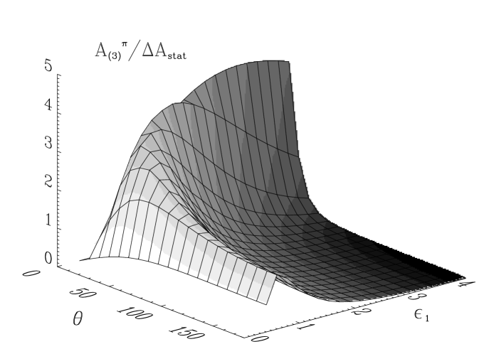
FIG. 7.: As above, a 3-D plot of $A_{(3)}/A_{\rm tot}\over\delta A_{\rm stat}/A_{\rm tot}$, versus both incident energy and electron scattering angle. (The shading is determined by the value of $\Delta_{(3)}^{\pi}$, smaller values are shaded darker)

REFERENCES

- [1] M. J. Musolf et al., Phys. Rep. 239 (1994) 1.
- [2] “Precision Tests of the Standard Electroweak Model”, P. Langacker, Ed., World Scientific, Singapore (1995).
- [3] For some other recent discussions on the content of the nucleon, see, e.g., H. Noda, T. Tashiro, and T. Mizutani, Prog. Theor. Phys. 92 (1994) 909; R. Nag and S. Sanyal, J. Phys. G20 (1994) L125; X. D. Ji and J. A. Tang, Phys. Lett. B362 (1995) 182; K. Steininger and W. Weise, Phys. Lett. B329 (1996) 169; H. Holtmann, A. Szczurek, and J. Speth, Nucl. Phys. A596 (1996) 631; M.J. Ramsey-Musolf and H. Ito, Phys. Rev. C55 (1997) 3066; M.J. Musolf, H.-W. Hammer, and D. Drechsel, Phys. Rev. D55 (1997) 2741; P. Geiger and N. Isgur, Phys. Rev. D55 (1997) 299; H.-W. Hammer and M.J. Ramsey-Musolf, Phys. Lett. B416 (1998) 5; M.J. Ramsey-Musolf and H.-W. Hammer, preprint INT97-00-170 [hep-ph/9705409], to appear in Phys. Rev. Lett.
- [4] For a discussion of unitarity issues, see R. M. Davidson and N. C. Mukhopadhyay, Phys. Rev. D42 (1990) 20; R. M. Davidson, N. C. Mukhopadhyay, and R. S. Wittman, ibid., D43 (1991) 71.
- [5] K. M. Watson, Phys. Rev. 95 (1954) 228; E. Fermi, Supp. Nuovo Cim. 10 (1955) 17.
- [6] Y. Nambu and E. Schrauner, Phys. Rev. 128 (1962) 862; S. L. Adler and W. I. Weissberger, ibid. 169 (1968) 1392.
- [7] M. Khandakar and A. M. Sandorfi, Phys. Rev. D51 (1995) 3966, and refs. therein.
- [8] R. Beck et al., Phys. Rev. Lett. 78 (1997) 606.
- [9] C. Carlson, Phys. Rev. D34 (1986) 2704.
- [10] T. Kitagaki et al., Phys. Rev. D42 (1990) 1331.
- [11] S.P. Wells, “Measurement of the Parity-Violating Asymmetry in the Transition”, in Future Directions in Parity-Violation, Fifth Annual INT/Jefferson Lab Workshop, Seattle, WA, 1997, R. Carlini and M.J. Ramsey-Musolf eds. (unpublished).
- [12] Jefferson Laboratory experiment # E97-104, “Measurement of the Parity Violating Asymmetry in the N to Delta Transition”, S.P. Wells, N. Simicevic, and K. Johnston, spokespersons (1997).
- [13] D. R. T. Jones and S. T. Petcov, Phys. Lett. 91B (1980) 137.
- [14] R. N. Cahn and F. J. Gilman, Phys. Rev. D17 (1978) 1313.
- [15] M. J. Musolf and T. W. Donnelly, Nucl. Phys. A546 (1992) 509; ibid. A550 (1992) 564(E).
- [16] T. R. Hemmert, B. R. Holstein, and N. C. Mukhopadhyay, Phys. Rev. D51 (1995) 158.
- [17] R. M. Davidson and N. C. Mukhopadhyay, Phys. Rev. Lett. 79 (1997) 4509.
- [18] D. Leinweber, T. Draper, and R. M. Woloshyn, Phys. Rev. D46 (1992) 3067.
- [19] S. Capstick and G. Karl, Phys. Rev. D41 (1990) 2767.
- [20] H. -W. Hammer and D. Drechsel, Z. Phys. A353 (1995) 321.
- [21] M. J. Musolf and T. W. Donnelly, Z. Phys. C57 (1993) 559.
- [22] M. J. Musolf and B. R. Holstein, Phys. Lett. B242 (1990) 461.
- [23] S. L. Adler, Ann. Phys. 50 (1968) 89; Phys. Rev. D12 (1975) 2644.
- [24] S. J. Pollock, Ph. D. Thesis, Stanford University, (1987).
- [25] P. A. Zucker, Phys. Rev. D4 (1971) 3350.
- [26] T. W. Donnelly, J. Dubach, and I. Sick, Phys. Rev. C37 (1988) 2320; ibid., Nucl. Phys. A503 (1989) 589.
- [27] R.L. Walker, Phys. Rev. 182 (1969) 1729.
- [28] P. A. Schreiner and F. von Hippel, Nucl. Phys. B38 (1973) 333.
- [29] J. Líu, N. C. Mukhopadhyay and L. Zhang, Phys. Rev. C52, 1630 (1995); J. Líu, Ph. D. Thesis, Rensselaer, (1996).
- [30] G. Feinberg, Phys. Rev. D12 (1975) 3575.
- [31] J. D. Walecka, in “Muon Physics”, Vol. II, V. W. Hughes and C. S. Wu, Eds., Academic Press, New York (1975).
- [32] M. C. Noecker et al., Phys. Rev. Lett. 61 (1988) 310.
- [33] M. J. D Macpherson, K. P. Zetie, R. B. Warrington, D. N. Stacey, and J. P. Hoare, Phys. Rev. Lett. 67 (1991) 2784.
- [34] D. M. Meekhof, P. Vetter, P. K. Majumder, S. K. Lamoreaux, and E. N. Fortson, Phys. Rev. Lett. 71 (1993) 3442.
- [35] N. H. Edwards, S. J. Phipp, P. E. G. Baird, and S. Nakayama, Phys. Rev. Lett. 74 (1995) 2654.
- [36] P. A. Vetter, D. M. Meekhof, P. K. Majumder, S. K. Lamoreaux, and E. N. Fortson, Phys. Rev. Lett. 74 (1995) 2658.
- [37] C.S. Wood et al., Science 275 (1997) 1759.
- [38] W. J. Marciano and A. Sirlin, Phys. Rev. D27 (1983) 552.
- [39] W. J. Marciano and A. Sirlin, Phys. Rev. D29 (1984) 75.
- [40] M. E. Peskin and T. Takeuchi, Phys. Rev. Lett. 65 (1990) 964.
- [41] W. J. Marciano and J. L. Rosner, Phys. Rev. Lett. 65 (1990) 2963.
- [42] M. Golden and L. Randall, Nucl. Phys. B361 (1991) 3.
- [43] J. L. Rosner, Phys. Rev. D53 (1996) 2724.
- [44] J.L. Rosner, Univ. of Chicago preprint # EFI-97-18 (1997) [hep-ph/970431].
- [45] M. K. Pillai et al., CDF Collaboration, meeting of the Division of Particles and Fields, American Physical Society, (August 1996).
- [46] D. London and J. L. Rosner, Phys. Rev. D34 (1986) 1530.
- [47] P. Langacker, M. Luo, A.K. Mann, Rev. Mod. Phys. 64 (1992) 87.
- [48] H1 Collaboration, Z. Phys. C74 (1997) 191.
- [49] Zeus Collaboration, Z. Phys. C74 (1997) 207.
- [50] P. Frampton, “Leptoquarks”, talk given at Beyond the Standard Model V, May 4, 1997, Balestrand, Norway [hep-ph/9706220] and references therein.
- [51] E. Eichter, K. D. Lane, and M. E. Peskin, Phys. Rev. Lett. 50 (1983) 811.
- [52] A.E. Nelson, Phys. Rev. Lett. 78 (1997) 4159.
- [53] L. Zhang and N. C. Mukhopadhyay, Phys. Rev. D50 (1994) 4668; L. Zhang and N. C. Mukhopadhyay, to be published.
- [54] E. Jenkins and A. V. Manohar, Phys. Lett. B259 (1991) 353; D. B. Leinweber, Phys. Rev. D53 (1996) 5115.
- [55] V. Bernard, N. Kaiser, and U-G. Meißner, Phys.Lett. B331 (1994) 137.
- [56] M. N. Butler, M. J. Savage, and R. P. Springer, Nucl. Phys. B399 (1993) 69; M. Napsuciale and J. L. Lucio, Nucl. Phys. B494 (1997) 260; T.R. Hemmert, B.R. Holstein, and J. Kambor, Phys. Lett. B395 (1997) 89.
- [57] L.A. Ahrens et al., Phys. Rev. D35 (1987) 18.
- [58] S. -P. Li, E. M. Henley, and W. -Y. P. Hwang, Ann. Phys. 143 (1982) 372.
- [59] V. Bernard, N. Kaiser, and U.-G. Meißner, Phys. Lett. B282 (1992) 448.
- [60] V. Burkert and R. Minehart, CEBAF proposal No. E-89-037, and private communications (1996).
- [61] N. C. Mukhopadhyay, to be published.
- [62] M. J. Musolf and B. R. Holstein, Phys. Rev. D43 (1991) 2956.
- [63] D.H. Beck, “Meson Exchange and Neutral Weak Currents” , in Workshop on CEBAF at Higher Energies, N. Isgur and P. Stoler, Eds., CEBAF, Newport News, VA (April 1994)
- [64] F. W. Brasse et al., Nucl. Phys. B110 (1976) 413.
- [65] F. Halzen and A. D. Martin, Quarks and Leptons, John Wiley & Sons, New York, (1984).
- [66] P. Salin, Nuovo Cim. A38 (1967) 506.
- [67] J. Bijtebiar, Nucl.Phys. B21 (1970) 158.
- [68] L. M. Nath, K. Schilcher, and M. Kretzschmar, Phys. Rev. D25 (1982) 2300.
- [69] F. Ravndal, Nuovo Cim. A18 (1973) 385.
- [70] A. Le Yaouanc et al., Phys. Rev. D15 (1977) 2447.
- [71] J. G. Körner, T. Kobayashi, and C. Avilez, Phys. Rev. D18 (1978) 3178.
- [72] M. J. Ramsey-Musolf, to be published.
- [73] T. Abdullah and F. Close, Phys. Rev. D5 (1972) 2332.