Reconstructing the Source in Heavy Ion Collisions from Particle Interferometry

Abstract

The preliminary CERN SPS NA49 Pb+Pb 158 GeV/A one- and two-particle $h^{-}$-spectra at mid-rapidity are consistent with a source of temperature $T\approx 130$ MeV, lifetime $\tau_{0}\approx 9$ fm/c, transverse flow $\eta_{f}\approx 0.35$, and a transverse geometric size which is twice as large as the cold Pb nucleus.

1 Introduction

Hadronic one- and two-particle spectra provide for each particle species information about the phase-space distribution $S(x,K)$ of the hadronic emission region [1]. Once reconstructed from the measured spectra, $S(x,K)$ allows to distinguish between different dynamical scenarios of heavy ion collisions. It provides an experiment-based starting point for a dynamical back extrapolation into the hot and dense early stage of the collision, where quarks and gluons are expected to be the relevant physical degrees of freedom.

Our reconstruction of $S(x,K)$ is based on the hadronic one- and two-particle spectra

$$E{dN\over d^{3}p} = \int d^{4}x\,S(x,p)=\textstyle{1\over 2\pi}{d^{2}N\over p_{t}\,dp_{t}\,dy}[1+2\sum_{n=1}^{\infty}v_{n}\cos n(\phi-\psi_{R})]\,,$$ (1)

$$C({\bf K},{\bf q}) = 1+{{|\int d^{4}x\,S(x,K)\,e^{iq\cdot x}|^{2}}\over{\int d^{4}xS(x,p_{1})\,\int d^{4}y\,S(y,p_{2})}}=1+\lambda\exp\left[-\sum_{ij}R_{ij}^{2}({\bf K})\,{\bf q}_{i}\,{\bf q}_{j}\right]\,.$$ (2)

The triple-differential hadronic one-particle spectrum (1) tests the momentum-dependence of $S(x,K)$ only. Its azimuthal $\phi$-dependence with respect to the reaction plane $\psi_{R}$ is parametrized by the harmonic coefficients $v_{n}$ [2]. Information about the space-time structure of $S(x,K)$ can be obtained from the relative momentum dependence of the two-particle correlator $C({\bf K},{\bf q})$, ${\bf q}={\bf p}_{1}-{\bf p}_{2}$. This ${\bf q}$-dependence is usually parametrized via the Hanbury-Brown Twiss (HBT) radius parameters $R_{ij}^{2}({\bf K})$ which depend on the average pair momentum ${\bf K}=\textstyle{1\over 2}({\bf p}_{1}+{\bf p}_{2})$. Depending on the Gaussian parametrization adopted, the indices $i$, $j$ in (2) run either over the Cartesian directions long (parallel to the beam), out (parallel to the transverse component ${\bf K}_{\perp}$) and side, or over the corresponding Yano-Koonin coordinates $q_{\perp}=\sqrt{q_{o}^{2}+q_{s}^{2}}$, $q_{3}$ and $q^{0}={\bf q}\cdot{\bf K}/K_{0}$  [1].

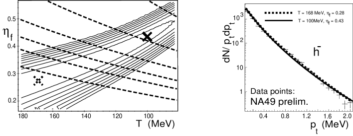
Figure 1: LHS: $\chi^{2}$ contour plot of a fit to the NA49 [3] $h^{-}$-spectrum. Dashed lines are for constant values of $\eta_{f}^{2}/T$. RHS: different combinations of temperature $T$ and transverse flow $\eta_{f}$ account for the same one-particle slope.

2 Reconstructing an azimuthally symmetric source

A typical data analysis starts from a simple ansatz for the phase space distribution $S(x,K)$ in terms of very few, physically intuitive fit parameters, [1, 4]:

$$S_{\pi}(x,p) = S_{\pi}^{\rm dir}(x,p)+\sum_{R}S_{R\to\pi}(x,p)\,,$$ (3)

$$S^{\rm dir}_{i}(x,P) = \textstyle{2J_{i}+1\over(2\pi)^{3}}\,P{\cdot}n(x)\,\exp{\left(-{P\cdot u(x)\over T}\right)}\,\exp\left(-{r^{2}\over 2R^{2}}-{\eta^{2}\over 2(\Delta\eta)^{2}}-{(\tau-\tau_{0})^{2}\over 2(\Delta\tau)^{2}}\right)\,.$$ (4)

This model e.g. assumes local thermalization at freeze-out with temperature $T$ within a space-time region of transverse Gaussian width $R$, emission duration $\Delta\tau$, longitudinal extension $\tau_{0}\Delta\eta$, where $\eta={1\over 2}\ln{[(t+z)/(t-z)]}$, and average emission time $\tau_{0}$. The model allows for dynamical source correlations via the hydrodynamic flow $4$-velocity $u_{\mu}(x)$. We assume a linear transverse flow profile $\eta_{t}(r)=\eta_{f}\left({r\over R}\right)$ with variable strength $\eta_{f}$, and Bjorken scaling of the flow component in the longitudinal direction, $v_{l}=z/t$, $\eta_{l}\equiv{1\over 2}\ln[(1+v_{l})/(1-v_{l})]=\eta$. Resonances are produced in thermal abundances with proper spin degeneracy $2J_{i}+1$ for each particle species $i$. Their contribution to the pion yield is obtained by propagating them along their classical path $x^{\mu}=X^{\mu}+{P^{\mu}\over M}\tau$ according to an exponential decay law [4],

$$S_{R\to\pi}(x,p)=\int_{\bf R}\,\int d^{4}X\,\int d\tau\,\Gamma e^{-\Gamma\tau}\,\delta^{(4)}\textstyle{\left[x-\left(X+{P\over M}\tau\right)\right]}S_{R}^{\rm dir}(X,P)\,,$$ (5)

where $\int_{\bf R}$ is the integral over the available resonance phase space for isotropic decays. We include all pion decay channels of $\rho$, $\Delta$, $K^{*}$, $\Sigma^{*}$, $\omega$, $\eta$, $\eta^{\prime}$, $K_{S}^{0}$, $\Sigma$ and $\Lambda$ with branching ratios larger than 5 percent.

Figure 2: Yano-Koonin-Podgoretskii HBT-radius parameters. The preliminary NA49 Pb+Pb data [5] are for $h^{+}h^{+}$ (squares) and $h^{-}h^{-}$ (diamonds) correlations.

The model parameters $T$, $\eta_{f}$, $R$, $\Delta\eta$, $\Delta\tau$, $\tau_{0}$ can then be determined via the following strategy:

1. transverse one-particle spectrum $dN/dM_{\perp}^{2}$ determines blue-shifted temperature $T_{\rm eff}$:
   The slope of $dN/dM_{\perp}^{2}$ is essentially given by $T_{\rm eff}=T\sqrt{(1+\eta_{f})/(1-\eta_{f})}$. Hence, different combinations of $T$ and $\eta_{f}$ can account for the same data, see Fig. 1.

2. $dN/dM_{\perp}^{2}$ and $R_{\perp}(M_{\perp})$ disentangle temperature and transverse flow. $R_{\perp}$ fixes transverse extension $R$:
   The $M_{\perp}$-slope of $R_{\perp}$ is proportional to $\eta_{f}^{2}/T$, $R_{\perp}^{2}\approx R^{2}/(1+M_{\perp}\eta_{f}^{2}/T)$ [6, 7]. This slope allows in combination with $dN/dM_{\perp}^{2}$ to specify $T$ and $\eta_{f}$, see Fig. 2. The overall size of $R_{\perp}$ determines the Gaussian width $R$. We find $\eta_{f}\approx 0.35$, $T\approx 130$ MeV, $R\approx 7$ fm.

3. $R_{\parallel}$ determines $\tau_{0}$, width of rapidity distribution $dN/dY$ determines $\Delta\eta$:
   In principle, $R_{\parallel}$ depends on $\tau_{0}$, $\Delta\eta$ and $\Delta\tau$ [7]. We have fixed $\Delta\eta=1.3$ by matching the width of the pion rapidity distribution. The data then favour clearly a lifetime of $\tau_{0}\approx 9$ fm/c (see Fig. 2) but are not very sensitive to the emission duration $\Delta\tau$ [8]. The present plots are obtained with $\Delta\tau=1.5$ fm/c.

4. $R_{0}$ discards opaque sources:
   For the model (3-5), the YKP-parameter $R_{0}$ is mainly sensitive to the temporal aspects of the source. The large statistical uncertainties for $R_{0}$ do not allow to constrain the model parameter space further, see Fig. 2. Models of opaque sources including an opacity factor in (4) are excluded already by the present data [8].

The radius of a cold Pb nucleus corresponds to $R_{\rm Pb}({\rm cold})\approx 3.5$ fm in the Gaussian parametrization (4), i.e., the experimental data indicate a very large source $R\approx 2\,R_{\rm Pb}({\rm cold})$. This is dynamically consistent with a collision scenario in which the initially produced pressure gradients result in a significant transverse flow $\eta_{f}=0.35$, driving the expansion of the system over a time of 9 fm/c to twice its initial size. The temperature may have decreased substantially during this expansion; the data indicate 130 MeV at freeze-out. These conclusions are further supported by the analysis presented by G. Roland [9], which is based on approximate analytical formulas. We have extracted the model parameters by comparison to numerical model calculations, following the above strategy. They are not obtained from a simultaneous fit to all observables, and hence we do not quote errors.

3 Particle interferometry for collisions with finite impact parameter

The reaction plane analysis of triple-differential one-particle spectra (1) has been discussed extensively in this conference e.g. by A. Poskanzer, J.-Y. Ollitrault, and S. Voloshin. The general strategy for linking this analysis to an azimuthally sensitive particle interferometry is based on the $\Phi$-dependence of the HBT-radii [10], where $\Phi$ measures the azimuthal angle of $\vec{\bf K}_{\perp}$ relative to the reaction plane,

$$R_{ij}^{2}(K_{\perp},\Phi,Y)=R_{ij,0}^{2}(K_{\perp},Y)+2\sum_{n=1}^{\infty}{R^{c}_{ij,n}}^{2}(K_{\perp},Y)\cos n\Phi+2\sum_{n=1}^{\infty}{R^{s}_{ij,n}}^{2}(K_{\perp},Y)\sin n\Phi\,.$$ (6)

Here, the many harmonic coefficients $R^{*}_{ij,*}$ make a direct comparison to experimental data impossible. However, various relations hold amongst these coefficients, since the leading anisotropy in realistic source models $S(x,K)$ can be quantified by very few parameters only. Using the symmetries of the system and assuming that elliptic deformations dominate we find [10]

$$0 \approx {R_{l,m}^{c}}^{2}\approx{R_{l,m}^{s}}^{2}\approx{R_{ol,m}^{c}}^{2}\approx{R_{ol,m}^{s}}^{2}\approx{R_{sl,m}^{c}}^{2}\approx{R_{sl,m}^{s}}^{2}\qquad\,,m\geq 1\,,$$ (7)

$$\alpha_{1} \approx {1\over 3}{R_{o,1}^{c}}^{2}\,\approx\,{R_{s,1}^{c}}^{2}\,\approx\,-{R_{os,1}^{s}}^{2}\,,$$ (8)

$$\alpha_{2} \approx -{R_{o,2}^{c}}^{2}\,\approx{R_{s,2}^{c}}^{2}\,\approx\,{R_{os,2}^{s}}^{2}\,.$$ (9)

A violation of Eqs. (8)-(9) by experiment would indicate strong higher order deformations and rule out many model scenarios. On the basis of Eqs. (7)-(9), an azimuthally sensitive parametrization of the two-particle correlator involves only two additional fit parameters,

$$C_{\psi_{R}}({\bf K},{\bf q}) \approx 1+\lambda\exp[-{R_{o,0}}^{2}\,q_{o}^{2}-{R_{s,0}}^{2}\,q_{s}^{2}-{R_{l,0}}^{2}\,q_{l}^{2}-2\,{R_{ol,0}}^{2}\,q_{o}q_{l}]\,$$ (10)

$$\qquad\times\exp\big{[}-\alpha_{1}\,(3\,q_{o}^{2}+q_{s}^{2})\,\cos(\Phi-\psi_{R})\,+2\alpha_{1}\,q_{o}q_{s}\sin(\Phi-\psi_{R})\big{]}$$

$$\qquad\times\exp\big{[}-\alpha_{2}(q_{o}^{2}-q_{s}^{2})\cos 2(\Phi-\psi_{R})+2\,\alpha_{2}q_{o}q_{s}\sin 2(\Phi-\psi_{R})\big{]}\,.$$

The anisotropy parameter $\alpha_{1}$ vanishes at mid-rapidity or if the source contains no dynamical correlations. It characterizes anisotropic dynamics. The parameter $\alpha_{2}$ characterizes the elliptic geometry. The parameters $\alpha_{1}$ and $\alpha_{2}$ can be determined from event samples in spite of the uncertainty in the eventwise reconstruction of the reaction plane. For details, see Ref. [10].

This work is supported by BMBF, DAAD, DFG and GSI.

References

- [1] U. Heinz, nucl-th/9609029.
- [2] S.A. Voloshin and Y. Zhang, Z. Phys. C70 (1996) 665.
- [3] P. Jones for the NA49 Coll., Quark Matter ’96, Nucl. Phys. A610 (1996) 188c.
- [4] U.A. Wiedemann and U. Heinz, Phys. Rev. C56 (1997) 3265; ibidem R610.
- [5] H. Appelshäuser, NA49 PhD-thesis.
- [6] S. Chapman, R. Nix and U. Heinz, Phys. Rev. C52 (1995) 2694.
- [7] U.A. Wiedemann, P. Scotto and U. Heinz, Phys. Rev. C53 (1996) 918.
- [8] B. Tomášik and U. Heinz, nucl-th/9707001, and poster at this conference.
- [9] G. Roland for the NA49 Coll., these proceedings.
- [10] U.A. Wiedemann, Phys. Rev. C57 (1998) 266.