FERMIONIC MOLECULAR DYNAMICS AND SHORT RANGE CORRELATIONS

Fermionic Molecular Dynamics (FMD) models a system of fermions by means of many–body states which are composed of antisymmetrized products of single–particle states. These consist of one or several Gaussians localized in coordinate and momentum space. The parameters specifying them are the dynamical variables of the model. As the repulsive core of the nucleon–nucleon interaction induces short range correlations which cannot be accommodated by a Slater determinant, a novel approach, the unitary correlation operator method (UCOM), is applied. The unitary correlator moves two particles away from each other whenever their relative distance is within the repulsive core. The time–dependent variational principle yields the equations of motion for the variables. Energies of the stationary ground states are calculated and compared to exact many–body results for nuclei up to ⁴⁸Ca. Time–dependent solutions are shown for collisions between nuclei.

1 Concept

The general concept of Fermionic Molecular Dynamics (FMD) $\!{}^{{\bf?}}$ is to describe a system of fermions by a many–body trial state which is antisymmetric with respect to particle exchange (”Fermionic”). The attribute ”Molecular” indicates that the individual single–particle states, from which Slater determinants are formed, are wave packets localized in coordinate as well as momentum space. Hence they are the quantum analogue to classical points in phase space. The time evolution of the parameters which specify the many–body state, like mean positions, mean momenta, or spin orientations of the wave packets, is obtained from the time–dependent variational principle (”Dynamics”). A closely related model is AMD $\!{}^{{\bf?}}$ which follows the same concept but differs from FMD in several aspects.

1.1 The trial state

In FMD the trial states are antisymmetrized $A$–body states

$$\,|{Q}\rangle=C{\cal A}\;\,|{\hat{q}_{1}}\rangle\otimes\,|{\hat{q}_{2}}\rangle\otimes\cdots\otimes\,|{\hat{q}_{A}}\rangle\ ,$$ (1)

where $Q$ denotes the set of all subsets $\hat{q}_{k}$ which specify the parameters of the single–particle states $\,|{\hat{q}_{k}}\rangle$. These are Gaussians, localized in phase space, or superpositions of several Gaussians. In this case $\hat{q}_{k}$ includes in addition to the complex parameters mean positions, widths and two–component spinors also the complex amplitude for each Gaussian. In general $\,|{Q}\rangle$ can be a superposition of correlated Slater determinants, then the set $Q$ includes also the configuration–mixing amplitudes.

${\cal A}$ is the projector onto the antisymmetric Hilbert space of fermions. $C$ is a unitary correlation operator which takes care of the short range correlations as explained in subsection 2.

1.2 The time–dependent variational principle

The equations of motion for all parameters in $Q=\{q_{\nu};\nu=1,2,\cdots,N\}$ are obtained from the time–dependent variational principle

$$\delta\int_{t_{1}}^{t_{2}}\!\!{\mathrm{d}}t\;\langle{Q(t)}|\,\;i\frac{\mathrm{d}}{{\mathrm{d}}t}\>-H\;\,|{Q(t)}\rangle\ =\ 0\ ,$$ (2)

where the variation is taken with respect to all individual parameters $q_{\mu}$ or their complex conjugate $q_{\mu}^{*}$. The resulting equtions of motion are

$$\langle{\frac{\partial{}}{\partial{q_{\mu}^{*}}}\>Q(t)}|\,\;{\mathrm{i}}\,\frac{\mathrm{d}}{{\mathrm{d}}t}\>-H\;\,|{Q(t)}\rangle=\langle{\frac{\partial{}}{\partial{q_{\mu}^{*}}}\>Q(t)}|\,{\mathrm{i}}\,\!\!\sum_{\nu}\dot{q}_{\nu}\frac{\partial{}}{\partial{q_{\nu}}}\>-H\;\,|{Q(t)}\rangle\ =\ 0\ .$$ (3)

The physical meaning of these equations is that the deviation of the exact state from the approximate $\,|{Q(t+{\mathrm{d}}t)}\rangle$, which develops during a time interval d$t$,

$$\,|{Error(t+{\mathrm{d}}t)}\rangle \equiv \;\big{(}\>1-{\mathrm{i}}\,{\mathrm{d}}t\;H\>\big{)}\,|{Q(t)}\rangle-\,|{Q(t+{\mathrm{d}}t)}\rangle$$ (4)

$$= {\mathrm{i}}\,{\mathrm{d}}t\big{(}\;{\mathrm{i}}\,\!\!\sum_{\nu}\dot{q}_{\nu}\frac{\partial{}}{\partial{q_{\nu}}}\>-H\;\big{)}\,|{Q(t)}\rangle$$ (5)

is orthogonal to the tangent $\langle{\frac{\partial{}}{\partial{q_{\mu}^{*}}}\>Q(t)}|\,^{\dagger}=\,|{\frac{\partial{}}{\partial{q_{\mu}}}\>Q(t)}\rangle\equiv\frac{\partial{}}{\partial{q_{\mu}}}\>\!\,|{Q(t)}\rangle$ at each time $t$, as can be seen by comparing Eq. (5) with (3). In other words the variational principle chooses the best $\,|{Q(t+{\mathrm{d}}t)}\rangle$ within the manifold $\,|{Q}\rangle$.

Stationary solutions of the variational principle (2), ground states for example, imply

$$\langle{\frac{\partial{}}{\partial{q_{\mu}^{*}}}\>Q(t)}|\,\;H\;\,|{Q(t)}\rangle=0\ .$$ (6)

1.3 Quantum–branching

If one wants to allow the time evolution to deviate from $\,|{Q(t)}\rangle$ without increasing the degrees of freedom one may take the operator

$$\Delta V(t)\equiv\big{(}\;{\mathrm{i}}\,\!\!\sum_{\nu}\dot{q}_{\nu}\frac{\partial{}}{\partial{q_{\nu}}}\>-H\;\big{)}$$ (7)

from Eq. (5) as a time–dependent pertubation to calculate transition amplitudes for quantum–branching away from $\,|{Q(t)}\rangle$. If the time evolution within the manifold happens to be exact, $\Delta V(t)\,|{Q(t)}\rangle=0$ and no branching occurs because all quantum physics is already in $\,|{Q(t)}\rangle$. The branching introduced by Ono and Horiuchi in AMD-V $\!{}^{{\bf?}}$ or the branching between energy eigenstates proposed by Onishi and Randrup $\!{}^{{\bf?}}$ may be investigated under this aspect.

2 The Unitary Correlation Operator Method (UCOM)

In nuclear physics this straightforward concept encounters a complicated Hamiltonian. Due to the complex structure of the nucleons and the mesons exchanged between them, the interaction depends on spin and isospin, is momemtum dependent and overall repulsive at short distances, see for example Ref. $\!{}^{{\bf?}}$. The properties of the Hamiltonian are of course intimately related to the choice of the trial state. The tensor part induces a strong correlation between the spins of a pair of nucleons and the direction of their relative distance $\!{}^{{\bf?}}$. The repulsion at short distances reduces the probability amplitude to find two nucleons close together. Both correlations cannot be described by a (antisymmetrized) product state. Therefore the most simple ansatz of a single Slater determinant has to be modified in order to incorporate the above mentioned correlations. In the following we sketch the new Unitary Correlation Operator Method (UCOM) which allows an approximate treatment of the short range repulsion even in time–dependent states.

Due to the short–ranged repulsive core in the nucleon–nucleon potential $V$ the many–body state is depleted as a function of the relative distance $x_{ij}=|\vec{x}_{i}-\vec{x}_{j}|$ for each pair $(ij)$ when they are close to each other. These short range correlations cannot be described by shell model states. The most common procedure to remedy this problem is Brueckner’s G-matrix method which replaces the bare $V$ by an effective interaction $G$. Another method is the Jastrow approach where the correlated ground state of the nucleus is assumed to be of the form $\prod_{i<j}f(x_{ij})\,|{\Phi}\rangle$ where $f(x_{ij})$ is a correlation factor which diminishes the probability to find two nucleons at small distances $x_{ij}$. We propose a new method $\!{}^{{\bf?}}$ in which the correlated state $\,|{Q}\rangle$ is obtained by a unitary transformation $C=\exp\{-{\mathrm{i}}\,G\}$. With respect to the choice of $G$ it differs from the work of K. Suzuki et al.$\!{}^{{\bf?}}$, where an effective interaction for the shell model is defined. In collisions between nuclei a preferred shell model space does not exist. Therefore, our definition of $G$ is not related to a given basis but to the behaviour of the relative wave function at small distances. The correlated state is given by

$$\,|{Q}\rangle=C\,|\widehat{{Q}}\rangle={\mathrm{e}}^{-{\mathrm{i}}\,G}\,|\widehat{{Q}}\rangle\;,$$ (8)

where the generator $G$ is a hermitean two–body operator which depends in general on the relative distance ${\!\vec{\,x}}_{ij}$, the relative momentum ${\!\vec{\,q}}_{ij}$, the spins and isospins of the two nucleons $\!{}^{{\bf?}}$. For sake of simplicity we sketch here only the case of a repulsive core without spin–isospin–dependence. In the application shown later $G$ depends on spin and isospin such that the different channels of a central interaction can be correlated individually.

The aim of $C$ is to push two nucleons away from each other whenever they get too close. The most simple ansatz which does that is

$$G=\frac{1}{2}\sum_{i<j}\left\{\left({\!\vec{\,q}}_{ij}\frac{{\!\vec{\,x}}_{ij}}{x_{ij}}\right)s(x_{ij})+s(x_{ij})\left(\frac{{\!\vec{\,x}}_{ij}}{x_{ij}}{\!\vec{\,q}}_{ij}\right)\right\}\ ,\ x_{ij}\equiv|{\!\vec{\,x}}_{ij}|\;.$$ (9)

$s(x_{ij})$ is roughly speaking the distance which the particles $i$ and $j$ are moved away from each other by $\exp\{-{\mathrm{i}}\,G\}$ if they are found at a distance $x_{ij}$ in $\,|\widehat{{Q}}\rangle$. $s(x_{ij})$ is largest if $x_{ij}$ lies inside the hard core and $s(x_{ij})\rightarrow 0$ if $x_{ij}$ is outside the repulsive interaction.

As $C^{\dagger}=C^{-1}$ is unitary one can correlate the states or equivalently the observables:

$$\langle{Q}|\,H\,|{Q}\rangle=\langle\widehat{{Q}}|\,C^{\dagger}H\,C\,|\widehat{{Q}}\rangle=\langle\widehat{{Q}}|\,C^{-1}H\,C\,|\widehat{{Q}}\rangle\equiv\langle\widehat{{Q}}|\,\widehat{H}\,|\widehat{{Q}}\rangle\,.$$ (10)

Closed expressions for the correlated relative wave function, the correlated potential and the correlated kinetic energy can be given by using the coordinate transformations $x_{ij}\rightarrow R_{\pm}(x_{ij})$ defined by

$$\int_{x}^{R_{\pm}(x)}\frac{{\mathrm{d}}\xi}{s(\xi)}=\pm 1\;.$$ (11)

For example the correlated potential is simply

$$\widehat{V}^{[2]}(x_{ij})\equiv C^{-1}V(x_{ij})\,C=V(C^{-1}x_{ij}\,C)=V(R_{+}(x_{ij}))\ .$$ (12)

Or a correlated relative wave–function can be expressed in terms of $R_{-}$ which is the inverse of $R_{+}$ as $({\!\vec{\,x}}\equiv{\!\vec{\,x}}_{i}-{\!\vec{\,x}}_{j}={\!\vec{\,x}}_{ij})$

$$\langle{{\!\vec{\,x}}}|{\phi}\rangle=\langle{{\!\vec{\,x}}}|\,C\,|\widehat{{\phi}}\rangle = \frac{R_{-}(x)}{x}\sqrt{\frac{\mathrm{d}}{{\mathrm{d}}x}R_{-}(x)}\;\;\langle{R_{-}(x)\frac{{\!\vec{\,x}}}{x}}|{\widehat{\phi}}\rangle$$ (13)

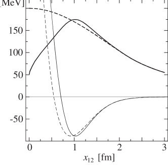
Figure 1: Uncorrelated state $\langle{{\!\vec{\,x}}_{12}}|{\widehat{\phi}}\rangle$(dashed line), correlated state $\langle{{\!\vec{\,x}}_{12}}|{\phi}\rangle$ (full line), Afnan–Tang potential $V(|{\!\vec{\,x}}_{12}|)$ (thin line) and correlated potential $\widehat{V}^{[2]}(|{\!\vec{\,x}}_{12}|)$ (thin dashed line) as a function of the relative distance $x_{12}=|{\!\vec{\,x}}_{12}|$.

Fig. 1 displays the radial dependence of the correlated and uncorrelated deuteron wave function together with the Afnan Tang S3 potential $\!{}^{{\bf?}}$. The functional form of $s(x)$ or equvalently of $R_{+}(x)$ is chosen such that the correlated state $\,|{\phi}\rangle$ for short distances equals the exact solution. The correlated kinetic energy is more involved as one has to calculate the correlated relative momentum $C^{-1}{\!\vec{\,q}}_{ij}\,C$. The details are given in Ref. $\!{}^{{\bf?}}$.

Once the correlator $C$ is adjusted to reproduce the two–body system at low energies (long wave length) one can calculate the ground state energies of nuclei by minimizing $\langle{Q}|\,H\,|{Q}\rangle=\langle\widehat{{Q}}|\,\widehat{H}\,|\widehat{{Q}}\rangle$ with respect to $\,|\widehat{{Q}}\rangle$ which in this application is a single Slater determinant composed of localized Gaussians (FMD).

Unlike the original Hamiltonian $H=T+V$, the correlated Hamiltonian

$$\widehat{H}\equiv C^{-1}H\,C=C^{-1}T\,C+C^{-1}V\,C=T+\!\widehat{T}^{[2]}+\!\widehat{V}^{[2]}+\!\widehat{T}^{[3]}+\!\widehat{V}^{[3]}+\cdots$$ (14)

is not a one– plus two–body operator anymore. It contains three–body and higher interactions because the generator $G$ is a two–body operator.

We calculate $\widehat{T}^{[2]}$ and $\widehat{V}^{[2]}$, which are functionals of $R_{+}$, analytically (for example as in Eq. (12)) and neglect irreducible three–body and higher terms in the expansion (14). This turns out to be a very good approximation at typical nuclear densities. Estimations of the three–body terms give corrections less than 5% of binding energy for the $\alpha$-particle $\!{}^{{\bf?}}$.

Figure 2: Energies for the modified Afnan-Tang S3 potential. Left columns: expectation values of kinetic energy $\,\langle\,{T}\,\rangle\,$, potential $\,\langle\,{V}\,\rangle\,$ and sum of both $\,\langle\,{H}\,\rangle\,$. Right columns: expectation values of correlated kinetic energy $\,\langle\,{T+\widehat{T}^{[2]}}\,\rangle\,$, correlated potential $\,\langle\,{\widehat{V}^{[2]}}\,\rangle\,$ and sum of both $\,\langle\,{\widehat{H}^{C2}}\,\rangle\,$. Arrows indicate the results of a Yakubovski calculation for ⁴He and of CBF calculations for ¹⁶O and for ^40,48Ca.

Fig. 2 compares uncorrelated (left columns) and correlated (right columns) energies. The correlated potential energy $\langle\widehat{{Q}}|\,\widehat{V}^{[2]}\,|\widehat{{Q}}\rangle$ (grey bars at negative values) is about twice the uncorrelated $\langle\widehat{{Q}}|\,V\,|\widehat{{Q}}\rangle$ in all nuclei. This gain in binding is counteracted by an increase in the kinetic energies (dark grey bars at positive values). Both together yield binding energies (black bars) which are within 8% deviation from results of Yakubovski calculations $\!{}^{{\bf?}}$ for $\mathrm{{}^{4}He}$ and CBF calculations $\!{}^{{\bf?},{\bf?}}$ for $\mathrm{{}^{16}O}$ and $\mathrm{{}^{40,48}Ca}$. This suprises since $\widehat{H}^{C2}=T+\widehat{T}^{[2]}+\widehat{V}^{[2]}$ is the same for all nuclei and not density dependent but it contains momentum dependent parts in the two–body part of the correlated kinetic energy $\widehat{T}^{[2]}$.

3 Ground states with several Gaussians

The Gaussian single–particle states do not describe properly the surface of nuclei because their tails do not fall off exponentially. Especially in the case of halo nuclei this is an important part of the physics. As Gaussians represent an overcomplete basis, any shape can be achieved by superimposing several Gaussians. In the following example we minimize the energy of ⁶He for a single Slater determinant with one Gaussian per particle and with two co–centered Gaussians with free widths and relative amplitudes. The resulting proton and neutron densities are displayed in Fig. 3 on a logarithmic scale. For the one Gaussian case (l.h.s.) the distribution of the neutrons is, as expected, wider than for the protons, but already with two Gaussians (r.h.s.) the trial state is much improved and exhibits nice exponential tails of different ranges. The binding energy increases by about 3.5 MeV and the ⁴He core which is distorted on the l.h.s. assumes again equal proton and neutron densities in the center. Three Gaussians do not improve the picture anymore. This example shows that a Gaussian basis may be a good representation for nuclear structure calculations. See for example also the contribution by M. Kamimura in these proceedings.

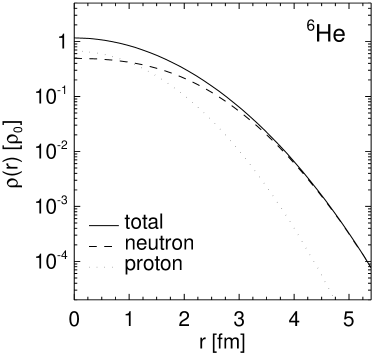
Figure 3: Proton and neutron densities of ⁶He with one Gaussian per aprticle (l.h.s.) and two Gaussians per particle (r.h.s)

We have also diagonalized the Hamilton matrix $\langle{Q_{k}}|\,H\,|{Q_{l}}\rangle$ within a subspace spanned by the nonorthogonal many–body states $\,|{Q_{k}}\rangle$. Dimensions of up to several hundred are feasible and for example eigenstates of total spin may be obtained by taking $\,|{Q_{k}}\rangle$ as rotated intrinsic states. See also contributions of S. Aoyama, N. Itagaki and S. Okabe or Y. Kanada-En’yo and H. Horiuchi or of K. Varga and Y. Suzuki in these proceedings.

4 The time–dependent case

In the time–dependent case one cannot be so ambitious as for ground states because all derivatives in Eq. 3 have to be calculated at each time step. Here we have to compromise and take only one Gaussian per particle and one Slater determinant. In addition the Hamiltonian is a simplified version of $\widehat{H}=C^{-1}HC$. We tried to adjust the parameters of the central $\widehat{H}$ such that ground state energies of nuclei up to mass 56 are reproduced within about 5% error. In doing that we found several Hamiltonians which describe similarly well the ground states but differ in their momentum dependence. A particular $\widehat{H}$ has two almost degenerate local energy minima in the manifold $\,|{Q}\rangle$. One minimum has states with an intrinsic cluster structure with narrow Gaussians placed at different positions in coordinate space, but centered in momentum space. The other shows co–centered Gaussians in cordinate space which are slightly displaced in momentum space, which resembles a shell model state.

Figure 4: Densities projected on scattering plane for ⁴⁰Ca+⁴⁰Ca collisions at b=2.75 fm and $E_{lab}$=35 AMeV. Initial nuclei in cluster and shell–model configurations. Crosses denote centroids of wave packets.

In Fig. 4 one sees that the two different types of states behave quite differently when they collide. In the left column, where two cluster states interact, multifragmentation is observed which could be characterized as shattering of the nuclei. Shell model states on cluster states produce also several fragments but in addition many nucleons are emitted. They are seen in the middle column as crosses (centroids of the packets) without surrounding contour lines, because the widths are already so large that the density distribution of the emitted nucleon has fallen below the lowest contour line. Finally, reactions with two shell model states (right column) look more like a deep inelastic collision with many nucleons evaporated because of the high excitation energy.

References

References

-
[1]
H. Feldmeier, J. Schnack,
Prog. Part. Nucl. Phys. 39, 393 (1997)
J. Schnack, H. Feldmeier, Nucl. Phys. A 601, 181 (1996)
H. Feldmeier, K. Bieler, J. Schnack, Nucl. Phys. A 586, 493 (1995)
H. Feldmeier, Nucl. Phys. A 515, 147 (1990) - [2] A. Ono, H. Horiuchi, Toshiki Maruyama and A. Onishi, Phys. Rev. Lett. 68, 2898 (1992), Prog. Theo. Phys. 87, 1185 (1992) and Phys. Rev. C 47, 2652 (1993) and these proceedings
- [3] A. Ono and H. Horiuchi, Phys. Rev. C 53, 2958 (1996) and these proceedings
- [4] A. Onishi and J. Randrup, Ann. Phys. 253, 279 (1997), Phys. Lett. B 394, 260 (1997) and these proceedings
- [5] R. Machleidt, Adv. Nucl. Phys. 19, 189 (1989)
- [6] J.L. Forest, V.R. Pandharipande et al, Phys. Rev. C 54, 646 (1996)
- [7] H. Feldmeier, T. Neff, R. Roth, J. Schnack, Preprint nucl-th/9709038; to be published in Nucl. Phys. A
-
[8]
K. Suzuki and R. Okamoto,
Prog. Theo. Phys. 92, 1045 (1994)
K. Suzuki, R.Okamoto and H. Kumagai, Phys. Rev. C 92, 1045 (1987)
and these proceedings - [9] I.R. Afnan, Y.C. Tang, Phys. Rev. 175, 1337 (1968)
- [10] H. Kamada, W. Glöckle, Nucl. Phys. A 548, 205 (1992)
- [11] G. Co’ et al, Nucl. Phys. A 549, 439 (1992)
- [12] F.A. de Saavedra et al, Nucl. Phys. A 605, 359 (1996)