FRAGMENTS IN GAUSSIAN WAVE-PACKET DYNAMICS
WITH AND WITHOUT CORRELATIONS

Abstract

Generalization of Gaussian trial wave functions in quantum molecular dynamics models is introduced, which allows for long-range correlations characteristic for composite nuclear fragments. We demonstrate a significant improvement in the description of light fragments with the correlations. Utilizing either type of Gaussian wave functions, with or without correlations, however, we find that we cannot describe fragment formation in a dynamic situation. Composite fragments are only produced in simulations if these fragments are present as clusters in the substructure of original nuclei. The difficulty is traced to the delocalization of wave functions during emission. Composite fragments are produced abundantly in the Gaussian molecular dynamics in the limit $\hbar\rightarrow 0$.

1 Correlated Molecular Dynamics

This talk is devoted to the description of fragments and their production in models of molecular dynamics with and without correlations. The considered correlations are long-range, such as characteristic for composite fragments, different from the short-range correlations discussed by H. Feldmeier. In the talk I shall, in sequence, discuss the introduction of correlations into molecular dynamics, describe the corresponding equations of motion, and discuss results for light clusters: deuteron and alpha. Subsequently, I shall turn to reactions and discuss results from simulating the decay of an excited system formed in reactions and results from collision calculations. I will end the talk with conclusions.

In quantum molecular dynamics models, the exact $N$-particle wave function of a system is replaced by a trial wave function used in the time-dependent variational principle. The different molecular approaches include Quantum Molecular Dynamics (QMD) [1, 2], Antisymmetrized Molecular Dynamics (AMD) [3], Extended Quantum Molecular Dynamics (EQMD) [4], and Fermion Molecular Dynamics (FMD) [5, 6]. A common feature of these approaches is that the trial wave function is a product, either antisymmetrized or not, of the single-particle Gaussian wave functions

$$\psi_{\nu}(\vec{x})=n\,\exp{\left(-a_{\nu}(\vec{x}-\vec{r}_{\nu})^{2}+i\,\vec{p}_{\nu}\,\vec{x}\right)}.$$ (1)

In effect of the product assumption, correlations between nucleons, other than those possibly induced by the antisymmetrization, vanish. The molecular approaches, otherwise, differ in some important details. Thus, QMD is the most classical of the approaches; the trial wave function is primarily used in the derivation. The width in the wave function (1) just acts to increase the range of effective interaction; the dynamics of the width is suppressed. No antisymmetrization is carried out and its effects are simulated using a Pauli potential. Within AMD the antisymmetrization is carried out. In EQMD the spreading of wave functions with time is taken into account. In FMD both the antisymmetrization is carried out and the width dynamics is included.

In any of the existing approaches, the center-of-mass wave function for any nucleon cluster is localized since, for a product wave function, the center of mass gets necessarily localized once the internal coordinates are localized. When a low-energy nucleon is emitted from a nucleus, it becomes delocalized getting rid of its localization energy. That has been, in fact, observed in the FMD simulations of reactions [6]. The delocalization, however, cannot take place in the molecular dynamics models for clusters, since their intrinsic state must stay localized. For light clusters such as deuterons or alphas, the cm localization energy is of the order of $\Delta E\sim(10-20)$ MeV. Given that temperatures are low when the fragments are expected to be produced in the low-energy reactions, $T<10$ MeV, the cm localization energy can result in significant suppression factors for the fragment emission, ${\rm e}^{-\Delta E/T}<(1/10-1/3)$.

Aiming at the description of fragment production in reactions, we considered ways of solving the problem of the artificial cm localization caused by the assumptions within the molecular dynamics. Let us first take a look at a deuteron Gaussian wave function, in which the intrinsic and cm motions are separated,

$$\exp{\Big{(}-\left({x_{1}+x_{2}\over\lambda^{\prime}}\right)^{2}\Big{)}}\,\exp{\Big{(}-\left({x_{1}-x_{2}\over\lambda}\right)^{2}\Big{)}}=\hskip 30.00005pt$$

$$\exp{\Big{(}-(x_{1}\,x_{2})\left(\begin{array}[]{cc}{1\over\lambda^{\prime 2}}+{1\over\lambda^{2}}&{1\over\lambda^{\prime 2}}-{1\over\lambda^{2}}\\[4.30554pt] {1\over\lambda^{\prime 2}}-{1\over\lambda^{2}}&{1\over\lambda^{\prime 2}}+{1\over\lambda^{2}}\end{array}\right)\left(\begin{array}[]{c}x_{1}\\[4.30554pt] x_{2}\end{array}\right)\Big{)}}\,.$$ (6)

The wave function that is a product of Gaussians in the cm and relative coordinates represents an exponential of the bilinear form in the coordinates of individual nucleons in (6). The case of a delocalized deuteron with total momentum tending to zero corresponds to $\lambda^{\prime}\rightarrow\infty$ in (6) and a small finite $\lambda$. The two nucleons are then correlated: the cm position may be anywhere in space but if one nucleon is found somewhere, then the other nucleon is within the distance of the order of $\lambda$ away from the first. On the other hand, the wave function reduces to a product of single-particle wave functions only when $\lambda=\lambda^{\prime}$.

Equation (6) suggests to use a generalized Gaussian as a trial wave function for $N$ particles,

$$\langle x_{1},\dots,x_{N}|\Psi\rangle={\cal N}\,\exp{\left[-A_{ij}\,(\vec{x}_{i}-\vec{r}_{i})\cdot(\vec{x}_{j}-\vec{r}_{j})+i\,\vec{p}_{i}\cdot\vec{x}_{i}\right]}\,,$$ (7)

where $A$ is the width matrix. The generalization (7) of the product of Gaussian single-particle wave functions allows for a full separation of the cm and intrinsic coordinates for any nucleon cluster and introduces correlations between different nucleons, $i\neq j$.

The width matrix $A$ in (7) is a symmetric, complex, $N\times N$ matrix with a positive-definite real part. The parameters $\{\vec{r}_{i}\}$ and $\{\vec{p}_{i}\}$, respectively, represent centroids and momenta for wave packets and the set $\{A_{ij},\vec{r}_{i},\vec{r}_{i}\}$ is related to various expectation values, including those that quantify the correlations, by

$$\langle\vec{x}_{i}\rangle = \vec{r}_{i}$$ (8)

$$\langle-i\,\vec{\nabla}_{i}\rangle = \vec{p}_{i}$$ (9)

$$\langle(\vec{x}_{i})_{a}\,(\vec{x}_{j})_{b}\rangle = (\vec{r}_{i})_{a}\,(\vec{r}_{j})_{b}+{\delta_{ab}\over 4}\,({\rm Re}A)^{-1}_{ij}$$ (10)

$$\langle i(\vec{\nabla}_{i})_{a}\,i(\vec{\nabla}_{j})_{b}\rangle = (\vec{p}_{i})_{a}\,(\vec{p}_{j})_{b}+\delta_{ab}\,(A^{\ast}\,({\rm Re}\,A)^{-1}\,A)_{ij}\,,$$ (11)

where $a$ and $b$ are indices for cartesian coordinates. For standard molecular dynamics, the width matrix is diagonal in particle indices

$$A_{ij}=A_{i}\,\delta_{ij}\,.$$ (12)

2 Equations of Motion

Equations of motion for the parameters $\{A_{ij},\vec{r}_{i},\vec{p}_{i}\}\equiv\{q_{\mu}\}$ follow from the variational principle

$$\delta\int_{t_{1}}^{t_{2}}dt\,\langle\Psi|i\,{d\over dt}-H|\Psi\rangle=0\,.$$ (13)

(For unrestricted variation, the principle yields the exact Schrödinger equation.) The equations take a form

$${\cal A}_{\nu\mu}\,\dot{q}_{\mu}=-{\partial\over\partial q_{\nu}}\,\langle H\rangle\,,$$ (14)

where the skew-symmetric matrix ${\cal A}$ represents the product of wave function derivatives

$${\cal A}_{\nu\mu}=2\,\,{\rm Im}\left\langle{\partial\over\partial q_{\nu}}\Psi\,\Bigg{|}\,{\partial\over\partial q_{\mu}}\Psi\right\rangle\,.$$ (15)

To solve the equations of motion, the matrix ${\cal A}$ needs to be inverted. When no antisymmetrization is carried out, the structure of the matrix is

$${\cal A}=\left(\begin{array}[]{cccc}0&{\cal B}&&\\ -{\cal B}&0&&\\ &&0&I\\ &&-I&0\end{array}\right)\,,$$ (16)

where the rows and columns refer, in sequence, to the parameter subspaces $\{{\rm Re}\,A\}$, $\{{\rm Im}\,A\}$, $\{r\}$, and $\{p\}$, $I$ is the identity in $N$-particle space, and ${\cal B}$ is a quadratic matrix of the dimension $N(N+1)/2$. The matrix ${\cal B}$ can be inverted analytically to yield a result in terms of the matrix elements of $A$. Because of this analytic inversion, the final effort in solving the equations of motion scales with particle number like $\sim N^{4}$; with the antisymmetrization the effort scales like $\sim N^{6}$.

Explicitly, the equations of motion take the form

$$\dot{\vec{r}}_{i}={\partial\langle H\rangle\over\partial\vec{p}_{i}}\,,\qquad\,\dot{\vec{p}}_{i}=-{\partial\langle H\rangle\over\partial\vec{r}_{i}}\,,$$ (17)

$${d\over dt}\,{\rm Re}\,A={\cal B}^{-1}\,{\partial\langle H\rangle\over\partial\,{\rm Im}\,A}\,,\qquad\,{d\over dt}\,{\rm Im}\,A=-{\cal B}^{-1}\,{\partial\langle H\rangle\over\partial\,{\rm Re}\,A}\,.\\$$ (18)

Contribution to the rhs of the equations for $A$ from the kinetic energy can be written as

$${\cal B}^{-1}\,{\partial\langle T\rangle\over\partial\,{\rm Im}\,A}={2\over m}\,{\rm Im}\,A^{2},\qquad{\cal B}^{-1}\,{\partial\langle T\rangle\over\partial\,{\rm Re}\,A}={2\over m}\,{\rm Re}\,A^{2}\,.\\$$ (19)

From (18) and (19), the $A$-matrix equation for free particles is

$$\dot{A}=-{2i\over m}\,A\,A$$ (20)

with a solution

$$A(t)=A_{0}\,\left(1+{2i\over m}\,(t-t_{0})\,A_{0}\right)^{-1}\,.$$ (21)

For initial conditions in a Gaussian form, the solution (21) represents an exact solution to the Schrödinger equation, with the spreading in time in the relative and cm coordinates for any set of nucleons. If the matrix $A$ is initially diagonal in these coordinates within the $N$-particle space, it will stay diagonal in these coordinates later on. When an interaction is included on the rhs of equations (18), it affects the evolution of the matrix elements and spreading for the intrinsic motion, but not for the cm motion. When, though, the matrix $A$ is always restricted to a diagonal form in the single-particle coordinates, then the intrinsic and cm motions get coupled. If spreading in the intrinsic coordinates is limited, so becomes the spreading in the cm coordinates. The intrinsic and cm energies are not separately conserved. Consequences of the coupling will be illustrated for light clusters.

3 Light Cluster Description

Figure 1

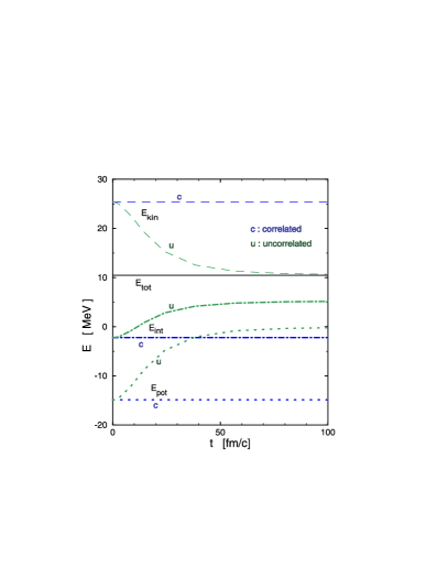
Figure 1: The dashed, solid, dash-dotted, and dotted lines show, respectively, the kinetic, total, internal, and potential energies, as a function of time, for a free deuteron in correlated ($c$) and and uncorrelated ($u$) dynamics.

shows the evolution of different energies for an isolated deuteron, within the standard uncorrelated wave-packet dynamics ($u$) and within the correlated dynamics ($c$) with nonvanishing off-diagonal matrix elements in $A$, following Eqs. (17) and (18). In the correlated dynamics the various energies for the deuteron stay constant. In the uncorrelated dynamics, the intrinsic motion taps on the energy from the cm motion. The intrinsic energy increases with time and at $t\sim 12$ fm/c the deuteron becomes unbound. Figure 2

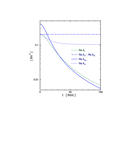
Figure 2: Evolution of the elements of the width matrix for the internal ground state of a free deuteron. The dashed lines shows the evolution of the element in the case of an uncorrelated wave function. The dash-dotted, solid, and dotted lines show, respectively, the evolution of the internal, center-of-mass, and diagonal elements in the case of a correlated wave function.

shows the evolution of the elements of the width matrix for the deuteron in the uncorrelated (dashed line) and correlated (remaining lines) dynamics. In the correlated dynamics the intrinsic width (corresponding to the dot-dashed line) stays constant, while the cm width (solid line) behaves like one for a free particle with twice the nucleon mass. The single-particle element $A_{11}$ (dotted line) drops with time and then stabilizes. In uncorrelated dynamics the single-particle element drops continuously; the deuteron dissolves.

The intrinsic state of an alpha particle initialized in the lowest state of intrinsic energy is stationary in the correlated wave-packet dynamics [7]. The cm state evolves in the same manner as the state for a particle with four times the nucleon mass. In the uncorrelated dynamics, on the other hand, the alpha particle, initialized as in the correlated dynamics, pulsates with time due to the energy exchange between the intrinsic and cm degrees of freedom. The energy acquired from the cm is not large enough in this case to dissolve the particle.

The results for the isolated particles show the benefits of using the correlated over the uncorrelated wave functions in the fragment description. We now turn to fragment production.

4 Reactions

Two types of simulations relevant for heavy-ion reactions will be discussed. One will be the decay of an excited system formed in the reactions. Second type will be complete reaction simulations followed from an initial state.

In our decay simulations we initialized the system (e.g. of mass $A=80$) in the state of a local thermal equilibrium with radial flow: The centroids $\vec{r}_{i}$ were randomly selected within a sphere of radius $R=(4\pi\rho/3)^{-1}$ ($R=5$ fm). The momenta $\vec{p}_{i}$ were selected randomly from a finite-$T$ Fermi-distribution ($T=5-12$ MeV). To every $\vec{p}_{i}$, a radial-flow momentum was added, proportional to position $\vec{p}_{i}\propto\vec{r}_{i}$ ($E_{col}=0-25$ MeV/nucleon). The width matrix was either taken proportional to unity ($\Delta x=1.9$ fm), or its diagonal and off-diagonal elements were generated randomly according to a distribution, or, finally, the matrix elements were equilibrated by keeping the system, at first, in a narrow external oscillator potential.

The initial (panel (a)) and late stages (panels (b)-(c)) of a system prepared in the described manner are shown in Fig. 3.

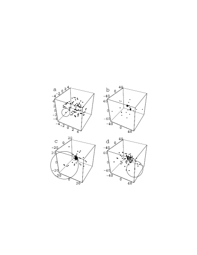
Figure 3: Particle centroids (dots) in the configuration space for $A=80$, in the initial state (a) and at $t=200$ fm/c for the static wave-packet width (b), and for the dynamic width matrix (c) and (d). In (c), the initial flow energy is lowered, compared to (b) and (d), by the initial energy content in the localization of the wave packets. The circles indicate rms radii of the most and least localized Gaussians. The axes show distances in fm.

In the calculations with a dynamic width matrix, the excited system emitted a number of nucleons but no clusters, neither of intermediate mass (IMF), nor lighter such as deuteron or $\alpha$ particle. There are some centroids in Fig. 3(c) that are close together, but the associated widths are so large that the interaction cannot hold the nucleons together and the centroids will separate with time.

When you get a final state of simulation without clusters you think first that it is a coincidence and you repeat the simulation with somewhat changed initial conditions. Again you find no clusters. Then you do that again and we have done that tens of times, maybe close to a hundred, and never saw any fragments, even an alpha. We observed, in fact little difference in the evolution for centroids between the uncorrelated dynamics and the correlated dynamics with the $A$-matrix initialized in a diagonal form. The simulations initialized with finite off-diagonal elements in $A$ also resulted in one residue and many emitted nucleons, but no IMFs or alphas.

As the primary reason for the lack of fragment production in the simulations we find the spreading of the wave packets with time. By the time the system reaches low densities and the fragments are expected to form, the packets get so spread out that the mutual interaction between the packets is unable to shrink them into clusters. Clearly, in the past, the production of IMFs and light clusters has been observed in the QMD calculations. Indeed, if we suppress the width dynamics (corresponding to $\hbar\rightarrow 0$ in our equations of motion), we begin to observe fragment production. This is illustrated in Fig. 3(b) that shows a late stage of the excited system evolved following the dynamics with a frozen wave-packet width. Two IMFs as well as two deuterons can be seen in the panel. Additional small clusters have been emitted before the shown time and left the displayed spatial region.

Our results on cluster production for the dynamic width matrix may seem in contradiction to the FMD results [6] with even multifragmentation events reported in nuclear collisions. Indeed, in our own simulations of collisions [7], we observed the production of clusters, but only if these were present in the substructure of original nuclei and did not manage to dissolve in the reaction. We never observed clusters that were formed in a reaction. For example, in the ground state of ¹²C, for our interaction, the centroids form three $\alpha$-type clusters of four nucleons each. If we collide two ¹²C nuclei, one or two of them may break up into three $\alpha$ particles. On the other hand, if we collide two ⁴⁰Ca nuclei, with no internal substructure, one or two residues are formed and many nucleons are emitted, but no clusters of intermediate mass.

5 Conclusions

In general, for uncorrelated wave functions, the internal state cannot be localized without localizing the center of mass. Thermal estimates indicate that the localization can act to suppress fragment production. In the dynamics, the use of uncorrelated wave functions leads to unphysical exchange of energy between the cm and intrinsic degrees of freedom. These deficiencies are eliminated in the dynamics utilizing correlated wave functions. The correlations that we have introduced are of such nature as expected for fragments and they allow for the separation of any number of nucleons in a wave function. The benefits of the correlated wave functions have been illustrated with the examples of deuteron and $\alpha$ particle.

Despite the benefits, in reaction simulations with dynamic widths, with or without correlations, we observe the cluster production only when the clusters are present in the initial state. The absence of new clusters is associated with large spreading of the wave function at the time when the reacting system expands and the new clusters should form. While there is nothing unphysical in the spreading of the wave function, as such, in the simulations, in reality the interaction would be capable of pinching portions of two or more packets and forming fragments out of the portions of these packets. The Gaussian parametrization of the wave function does not permit for the process.

On the basis of the reaction simulations, we conclude that, in a successful description of fragment production, the wave function must have a flexibility to change over distances comparable to the interaction range, at a time when the fragments are formed. The widths of the packets in AMD or QMD may already act to suppress the fragment production.

References

References

- [1] J. Aichelin and H. Stöcker, Phys. Lett. B176 (1986) 14.
- [2] T. Maruyama, A. Ohnishi, and H. Horiuchi, Phys. Rev. C42 (1990) 386.
- [3] A. Ono, H. Horiuchi, T. Maruyama and A. Ohnishi, Phys. Rev. Lett. 68 (1992) 2898.
- [4] T. Maruyama, K. Niita and A. Iwamoto, Phys. Rev. C53 (1996) 297.
- [5] H. Feldmeier, Nucl. Phys. A515 (1990) 147.
- [6] H. Feldmeier, K. Bieler and J. Schnack, Nucl. Phys. A586 (1995) 493.
- [7] D. Kiderlen and P. Danielewicz, Nucl. Phys. A620 (1997) 346.