A quantum kinetic equation for Fermi-systems including three-body correlations

Abstract

A single-time quantum transport equation, which includes effects beyond the quasiparticle approximation, is derived for Fermi-systems in the framework of non-equilibrium real-time Green’s functions theory. Ternary correlations are incorporated in the kinetic description via a cluster expansion for the self-energies (e.g., the transport vertex and the width) truncated at the level of three-body scattering amplitudes. A finite temperature/density formulation of the three-body problem is given. Corresponding three-body equations reduce to the well-known Faddeev equations in the vacuum limit. In equilibrium the equation of state contains virial corrections proportional to the third quantum virial coefficient.

I Introduction

A reliable description of the dynamics of Fermi-systems is commonly achieved in the quasiclassical (QC) limit, which is based on the concept of a classical particle moving in the mean field and along a classical trajectory between successive instantaneous collisions. The QC picture assumes a hierarchy of time-scales; the time-scales on which the renormalization of the excitation spectra and collisions occur are expected to be smaller than the mean time-scale between encounters of dressed quasiparticles. A similar assumption applies to the length-scales. As well known, such a separation is possible in the limiting cases of a classical dilute gas and a highly degenerate Fermi-liquid (for a review see, e.g.,  [1, 2]). The dynamical information in quasiclassical approximation (QCA) is contained in the single particle distribution function; the higher order distributions (determined form the BGKKY hierarchy) appear as time-dependent functionals of single particle distribution (for a review see, e.g.,  [3]). A second element of kinetic description of Fermi-systems is the quasiparticle approximation (QPA), which assumes a sharp functional dependence of the energies of the quasiparticles on their momenta. The QPA is sufficient to constrain the time-scale (but not the length-scale) hierarchy to the QC limit; it does not, however, appear to be a necessary condition.

The need of extension of kinetic description of Fermi-systems beyond QPA arises in a number of physical situations. An example is the excited nuclear matter produced in heavy-ion collision experiments at energies $\sim 100$ Mev/nucleon (for a review see, e.g.,  [4]). The expanding nuclear system traverses a broad region in the density-temperature plane and, in particular, the temperature could be of order the Fermi temperature. In such situations the spectral function of the single particle excitations acquires a finite width. If the half-width of the spectral function is small compared with the amplitude, the corrections to the QP picture are small, and the hierarchy of the time-scale still holds (in other words, a distinction can be made between the renormalization effect leading to the broading of the QP peak and the elementary collision events between the single particle excitations with renormalized spectra). The finite width of the spectral function introduces in the system correlations beyond the renormalization of the single particle spectrum, which lead to the so-called virial corrections, and in particular to formation of bound states (in nuclear collisions - deuterons [5, 6, 7], tritons, alpha particles, etc.) and off-mass-shell propagation (such as Landau-Pomeranchuk-Migdal effect in the particle radiation processes  [8]). Situation, similar to the one described above, is encountered also in the astrophysical context; e.g. in the finite temperature isospin asymmetical nuclear matter in the supernova collapse and proto-neutron stars.

The picture above suggests seeking a kinetic equation for Fermi-systems that accommodates the separation of the time and length-scales (and hence the QC approximation) while allowing for effects beyond the QPA. [Formally this means that the time-scales of variation of the self-energy functions (providing the renormalization and transport vertex) are small compared to the evolution time-scales for the propagators related to the quasiparticle distribution function].

Initial studies of the virial corrections to the Boltzmann equation were carried out using the density matrix approach  [9]; progress in this direction is represented by Snyder’s kinetic equation [10], where Bogoliubov’s ansatz of the weakening of the initial correlations is used to close the BGKKY hierarchy at the two-particle level. The partition of the virial corrections between the collision integral and the drift term is not unambiguous [11], however the kinetic equation reproduces the correct form of the lowest order (second) virial coefficient  [10]. The formation of the bound states and three-body processes within the density matrix approach has been considered e.g. by McLennan [12], Klimontovich et al  [13] and Röpke and Schulz [7], who derive coupled kinetic equations for a gas viewed as a reacting mixture of atoms and diatomic molecules or nucleons and their bound states (the authors do not consider the third virial coefficient, however).

The transport theory, which is based on the real-time Green’s functions formalism and is largely due to Kadanoff and Baym  [14] and Keldysh [15], provides an alternative to the density matrix approach, and allows systematic diagrammatic approximations to the propagators and self-energies. The reduction scheme for the double-time integro-differential Kadanoff-Baym equations for the Green’s functions to a single-time Boltzmann-type kinetic uses the QCA, which, as discussed above, separates the time and length-scales associated with individual collisions from those characterizing the inter-collision dynamics, and the QPA, which assumes a delta-shaped spectral function. The form and further approximations for the scattering-in and -out rates, represented by the Feynman diagrams of elementary scattering processes, vary considerably depending on the specifics of the dynamics and composition of the underlying system; cf., e.g.,  [16, 17, 18, 19].

The quantum kinetics beyond QPA has been addressed in a number of recent works [19, 20, 21, 22]. The memory effects in the non-Markovian kinetic equations, as shown in  [20], provide a sufficiently general description of correlations in quantum systems; the second order virial corrections emerge when the time-retarded spectral function is expanded to the next-to-leading order in retardation. This form of second-order quantum virial correction agrees with the equilibrium result derived for semiconductors [23], Coulomb plasmas  [24] and finite temperature nuclear matter  [25]. The second order virial corrections in the local-time description and for the electron-impurity system have been given in  [21] in terms of the next-to-leading order expansion of the spectral function with respect to the width  [22].

The solution of the three-body problem for an isolated system is well know, and is represented by the Faddeev [26] or AGS  [27] equations. The Kadanoff-Baym formalism has been applied to derive kinetic equations including triple collisions by Bezzerides and DuBois [28]; their study, however, has been restricted mainly to the Born approximation, and consequently the collision integrals contain singularities due to the non-Fredholm type kernels of the scattering amplitudes. A different motivation for studying the three-body equations comes from the problem of the imaginary nuclear potentials, where the 2-particle-hole channel dominates ground state correlations in nuclei  [29]. A self-consistent random phase approximation to the respective three-body problem at zero-temperature has been given in ref.  [29], while the the finite temperature discussion of the latter problem is contained in refs.  [17, 32] as an example of the application of the cutting rules for the multi-contour ordered Green’s functions due to Danielewicz  [17]. In the near-equilibrium situation the nucleon-deuteron system has been studied at finite temperatures in the AGS formulation in refs.  [33, 34].

Despite the progress mentioned above, the subject of the kinetics with three-body correlations needs further attention since (i) one would like to arrive at a kinetic equation which in the equilibrium limit leads to third order quantum virial corrections to the equation of state, (ii) the three-body collision processes should be free of singularities, therefore the appropriate Faddeev or AGS amplitudes should be used in the collision integrals (see also  [34]); (iii) the scattering amplitudes in the medium should reduce to the three-body Faddeev equations which are exact in the vacuum limit.

The purpose of this paper is to address these items and to provide a link between the kinetic description beyond the QPA and three-body correlations. We adopt the familiar methodology of next-to-leading order expansion of the spectral function with respect to the spectral width, however instead of the decomposition of Green’s functions into pole and off-pole terms [20, 21, 22], we use a decomposition in powers of the width. In the introduction to Section 2 we discuss the double-time kinetic equation and the gradient approximation to this equation (readers familiar with the formalism may skip this part of the section; the notation is as in Kadanoff and Baym [14]). Further subsections introduce the approximations to the spectral function, the method of decomposition of the diagrams in the QP and correlated parts, the Kadanoff-Baym ansatz and, finally, the single time kinetic equations. Section 3 derives the three-body equations at finite temperatures and densities. The transport vertex and the collision integrals are discussed in Section 4. The equilibrium limit of the kinetic regime and the third quantum virial coefficient are derived in Section 5. Section 6 contains a brief summary of our results.

II Dyson equations

Consider a non-relativistic Fermi-system interacting via two-body forces. The Hamiltonian of the system reads

$$H = \frac{1}{2m}\sum_{\sigma}\int d^{4}x\vec{\nabla}\psi_{\sigma}^{\dagger}(x)\vec{\nabla}\psi_{\sigma}(x)$$ (1)

$$+ \frac{1}{2}\sum_{\sigma\sigma^{\prime}}\int d^{4}xd^{4}x^{\prime}\psi_{\sigma}^{\dagger}(x)\psi_{\sigma^{\prime}}^{\dagger}(x^{\prime})V_{\sigma,\sigma^{\prime}}(x,x^{\prime})\psi_{\sigma^{\prime}}(x^{\prime})\psi_{\sigma}(x),$$ (2)

where $\psi_{\sigma}(x)$ are the Heisenberg field operators, $x=(\vec{r},t)$ is the space-time four vector, $\sigma$ stands for the internal degrees of freedom (spin, isospin, etc.). We shall use the matrix form of arrangement of time-contour ordered real time Green’s functions, which is particularly suited when initial correlations are absent. In this case the upper branch, $c_{-}$, runs from $-\infty$ to $\infty$ and the lower branch, $c_{+}$, from $\infty$ to $-\infty$. The initial correlation are commonly incorporated via the imaginary-time piece of the contour which accounts for the Kubo-Martin-Schwinger boundary condition  [17]. We shall neglect this piece in the further consideration. The single-particle propagator matrix is defined as

$${\mathchoice{{\hbox{\boldmath$\displaystyle\ G$}}}{{\hbox{\boldmath$\textstyle\ G$}}}{{\hbox{\boldmath$\scriptstyle\ G$}}}{{\hbox{\boldmath$\scriptscriptstyle\ G$}}}}_{12} = \left(\begin{array}[]{cc}G^{c}_{12}&G^{<}_{12}\\ G^{>}_{12}&{G}^{a}_{12}\end{array}\right)$$ (5)

$$= \left(\begin{array}[]{cc}-i\langle T\,\psi_{\sigma_{1}}(x_{1})\,\psi^{\dagger}_{\sigma_{2}}(x_{2})\rangle&i\langle\,\psi_{\sigma_{2}}^{\dagger}(x_{2})\,\psi_{\sigma_{1}}(x_{1})\rangle\\ -i\langle\,\psi_{\sigma_{1}}(x_{1})\,\psi_{\sigma_{2}}^{\dagger}(x_{2})\rangle&-i\langle\tilde{T}\,\psi_{\sigma_{1}}(x_{1})\,\psi_{\sigma_{2}}^{\dagger}(x_{2})\rangle\end{array}\right),$$ (8)

where the indexes $1,2...$ collectively denote the variables $(x_{1},\sigma_{1}),(x_{2},\sigma_{2})...$, the averaging is over a nonequilibrium state of the system; $T$ and $\tilde{T}$ are chronological and anti-chronological time ordering operators, respectively.

The perturbative expansion for the Green’s functions $\textstyle\ G$ can be arranged, as well known, in a manner similar to the ground state Feynman diagrammatic expansion utilizing Wick’s theorem. The single-particle propagator, therefore, obeys the Dyson equation

$${\mathchoice{{\hbox{\boldmath$\displaystyle\ G$}}}{{\hbox{\boldmath$\textstyle\ G$}}}{{\hbox{\boldmath$\scriptstyle\ G$}}}{{\hbox{\boldmath$\scriptscriptstyle\ G$}}}}_{12}={\mathchoice{{\hbox{\boldmath$\displaystyle\ G$}}}{{\hbox{\boldmath$\textstyle\ G$}}}{{\hbox{\boldmath$\scriptstyle\ G$}}}{{\hbox{\boldmath$\scriptscriptstyle\ G$}}}}_{12}^{(0)}+{\mathchoice{{\hbox{\boldmath$\displaystyle\ G$}}}{{\hbox{\boldmath$\textstyle\ G$}}}{{\hbox{\boldmath$\scriptstyle\ G$}}}{{\hbox{\boldmath$\scriptscriptstyle\ G$}}}}_{14}^{(0)}\otimes{\mathchoice{{\hbox{\boldmath$\displaystyle\Sigma$}}}{{\hbox{\boldmath$\textstyle\Sigma$}}}{{\hbox{\boldmath$\scriptstyle\Sigma$}}}{{\hbox{\boldmath$\scriptscriptstyle\Sigma$}}}}_{43}\otimes{\mathchoice{{\hbox{\boldmath$\displaystyle\ G$}}}{{\hbox{\boldmath$\textstyle\ G$}}}{{\hbox{\boldmath$\scriptstyle\ G$}}}{{\hbox{\boldmath$\scriptscriptstyle\ G$}}}}_{32}={\mathchoice{{\hbox{\boldmath$\displaystyle\ G$}}}{{\hbox{\boldmath$\textstyle\ G$}}}{{\hbox{\boldmath$\scriptstyle\ G$}}}{{\hbox{\boldmath$\scriptscriptstyle\ G$}}}}_{12}^{(0)}+{\mathchoice{{\hbox{\boldmath$\displaystyle\ G$}}}{{\hbox{\boldmath$\textstyle\ G$}}}{{\hbox{\boldmath$\scriptstyle\ G$}}}{{\hbox{\boldmath$\scriptscriptstyle\ G$}}}}_{14}\otimes{\mathchoice{{\hbox{\boldmath$\displaystyle\Sigma$}}}{{\hbox{\boldmath$\textstyle\Sigma$}}}{{\hbox{\boldmath$\scriptstyle\Sigma$}}}{{\hbox{\boldmath$\scriptscriptstyle\Sigma$}}}}_{43}\otimes{\mathchoice{{\hbox{\boldmath$\displaystyle\ G$}}}{{\hbox{\boldmath$\textstyle\ G$}}}{{\hbox{\boldmath$\scriptstyle\ G$}}}{{\hbox{\boldmath$\scriptscriptstyle\ G$}}}}_{32}^{(0)},$$ (9)

where the superscript $(0)$ refers to the free propagator, $\otimes$ stands for matrix multiplication along with the folding over the internal (repeated) indexes and the self-energy matrix $\textstyle\Sigma$ has a structure identical to eq. (5). The integro-differential form of the Dyson equation is obtained by acting the evolution operator ${\mathchoice{{\hbox{\boldmath$\displaystyle\ G$}}}{{\hbox{\boldmath$\textstyle\ G$}}}{{\hbox{\boldmath$\scriptstyle\ G$}}}{{\hbox{\boldmath$\scriptscriptstyle\ G$}}}}_{01}^{-1}=i\partial/\partial t_{1}+\nabla^{2}_{1}/2m$ on eq. (9) (the energy scales are measured relative to the fermion chemical potential) and employing the free-particle Dyson equation, ${\mathchoice{{\hbox{\boldmath$\displaystyle\ G$}}}{{\hbox{\boldmath$\textstyle\ G$}}}{{\hbox{\boldmath$\scriptstyle\ G$}}}{{\hbox{\boldmath$\scriptscriptstyle\ G$}}}}_{01}^{-1}\otimes{\mathchoice{{\hbox{\boldmath$\displaystyle\ G$}}}{{\hbox{\boldmath$\textstyle\ G$}}}{{\hbox{\boldmath$\scriptstyle\ G$}}}{{\hbox{\boldmath$\scriptscriptstyle\ G$}}}}_{12}^{(0)}=\mathchoice{{\hbox{\boldmath$\displaystyle\sigma$}}}{{\hbox{\boldmath$\textstyle\sigma$}}}{{\hbox{\boldmath$\scriptstyle\sigma$}}}{{\hbox{\boldmath$\scriptscriptstyle\sigma$}}}_{z}\,\,\delta^{(4)}(x_{1}-x_{2})$; here and below $\mathchoice{{\hbox{\boldmath$\displaystyle\sigma$}}}{{\hbox{\boldmath$\textstyle\sigma$}}}{{\hbox{\boldmath$\scriptstyle\sigma$}}}{{\hbox{\boldmath$\scriptscriptstyle\sigma$}}}_{i}$ ($i=x,y,z$) are the Pauli matrices and the subscript 0 refers to the evolution operator of free particle. Subtracting the resulting equation from its conjugate one finds

$$\left({\mathchoice{{\hbox{\boldmath$\displaystyle\ G$}}}{{\hbox{\boldmath$\textstyle\ G$}}}{{\hbox{\boldmath$\scriptstyle\ G$}}}{{\hbox{\boldmath$\scriptscriptstyle\ G$}}}}_{02}^{-1\,*}-{\mathchoice{{\hbox{\boldmath$\displaystyle\ G$}}}{{\hbox{\boldmath$\textstyle\ G$}}}{{\hbox{\boldmath$\scriptstyle\ G$}}}{{\hbox{\boldmath$\scriptscriptstyle\ G$}}}}_{01}^{-1}\right)\otimes{\mathchoice{{\hbox{\boldmath$\displaystyle\ G$}}}{{\hbox{\boldmath$\textstyle\ G$}}}{{\hbox{\boldmath$\scriptstyle\ G$}}}{{\hbox{\boldmath$\scriptscriptstyle\ G$}}}}_{12}={\mathchoice{{\hbox{\boldmath$\displaystyle\ G$}}}{{\hbox{\boldmath$\textstyle\ G$}}}{{\hbox{\boldmath$\scriptstyle\ G$}}}{{\hbox{\boldmath$\scriptscriptstyle\ G$}}}}_{13}\otimes{\mathchoice{{\hbox{\boldmath$\displaystyle\Sigma$}}}{{\hbox{\boldmath$\textstyle\Sigma$}}}{{\hbox{\boldmath$\scriptstyle\Sigma$}}}{{\hbox{\boldmath$\scriptscriptstyle\Sigma$}}}}_{32}\otimes\mathchoice{{\hbox{\boldmath$\displaystyle\sigma$}}}{{\hbox{\boldmath$\textstyle\sigma$}}}{{\hbox{\boldmath$\scriptstyle\sigma$}}}{{\hbox{\boldmath$\scriptscriptstyle\sigma$}}}_{z}-\mathchoice{{\hbox{\boldmath$\displaystyle\sigma$}}}{{\hbox{\boldmath$\textstyle\sigma$}}}{{\hbox{\boldmath$\scriptstyle\sigma$}}}{{\hbox{\boldmath$\scriptscriptstyle\sigma$}}}_{z}\otimes{\mathchoice{{\hbox{\boldmath$\displaystyle\Sigma$}}}{{\hbox{\boldmath$\textstyle\Sigma$}}}{{\hbox{\boldmath$\scriptstyle\Sigma$}}}{{\hbox{\boldmath$\scriptscriptstyle\Sigma$}}}}_{13}\otimes{\mathchoice{{\hbox{\boldmath$\displaystyle\ G$}}}{{\hbox{\boldmath$\textstyle\ G$}}}{{\hbox{\boldmath$\scriptstyle\ G$}}}{{\hbox{\boldmath$\scriptscriptstyle\ G$}}}}_{32}.$$ (10)

The matrix structure of the Green’s functions and the self-energies is not the optimal one yet. The retarded and advanced functions are preferable  [15, 17, 28], since they obey an integal equation in the lowest order of QCA. In terms of real parts of these functions (${\rm Re}\,G^{R}={\rm Re}\,G^{A}\equiv{\rm Re}\,G$ and ${\rm Re}\,\Sigma^{R}={\rm Re}\,\Sigma^{A}\equiv{\rm Re}\,\Sigma$) the kinetic equation, e.g., for the $G^{<}$ component is

$$\left[G_{03}^{-1}-{\rm Re}\Sigma_{13},G_{32}^{<}\right]-\left[{\rm Re}\,G_{13},\Sigma_{32}^{<}\right]=\frac{1}{2}\,\left\{G_{13}^{>},\Sigma_{32}^{<}\right\}-\frac{1}{2}\,\left\{\Sigma_{13}^{>},G_{32}^{<}\right\},$$ (11)

where $\left[~{},~{}\right]$ and $\left\{~{},~{}\right\}$ denote the commutator and anti-commutator, respectively, and a summation (integration) over repeated indexes is assumed. If the dynamics of the system permits a quasiclassical treatment, i.e., if the characteristic inter-collision length-scales are much greater than the inverse momenta and the relaxation times are much larger than the inverse frequencies, QCA can be applied by separating the slowly varying center-of-mass four-coordinates from the rapidly varying relative coordinates. Performing a Fourier transform with respect to the relative coordinates and keeping the first order gradients in the slow variable the QC Kadanoff-Baym kinetic equation reads

$$i\left\{{\rm Re}\,G^{-1},\,G^{<}\right\}_{\rm P.B.}+i\left\{\Sigma^{<}\,,{\rm Re}\,G\right\}_{\rm P.B.}=\Sigma^{<}G^{>}-\Sigma^{>}G^{<},$$ (12)

where all functions depend on the four energy-momentum vector $p\equiv(\omega,\,{\mathchoice{{\hbox{\boldmath$\displaystyle p$}}}{{\hbox{\boldmath$\textstyle p$}}}{{\hbox{\boldmath$\scriptstyle p$}}}{{\hbox{\boldmath$\scriptscriptstyle p$}}}})$, and the center of mass space-time vector $x$. Here the four-component Poisson bracket is defined as

$$\{f,\,g\}_{\rm P.B.}\equiv\frac{\partial f}{\partial\omega}\frac{\partial g}{\partial t}-\frac{\partial f}{\partial t}\frac{\partial g}{\partial\omega}-\frac{\partial f}{\partial\mathchoice{{\hbox{\boldmath$\displaystyle p$}}}{{\hbox{\boldmath$\textstyle p$}}}{{\hbox{\boldmath$\scriptstyle p$}}}{{\hbox{\boldmath$\scriptscriptstyle p$}}}}\frac{\partial g}{\partial\mathchoice{{\hbox{\boldmath$\displaystyle r$}}}{{\hbox{\boldmath$\textstyle r$}}}{{\hbox{\boldmath$\scriptstyle r$}}}{{\hbox{\boldmath$\scriptscriptstyle r$}}}}+\frac{\partial f}{\partial\mathchoice{{\hbox{\boldmath$\displaystyle r$}}}{{\hbox{\boldmath$\textstyle r$}}}{{\hbox{\boldmath$\scriptstyle r$}}}{{\hbox{\boldmath$\scriptscriptstyle r$}}}}\frac{\partial g}{\partial\mathchoice{{\hbox{\boldmath$\displaystyle p$}}}{{\hbox{\boldmath$\textstyle p$}}}{{\hbox{\boldmath$\scriptstyle p$}}}{{\hbox{\boldmath$\scriptscriptstyle p$}}}}.$$ (13)

Equation (12) is the starting point of the reduction of double time kinetic equation to the single time form; one recognizes the left-hand-side as a generalized drift term, while the right-hand-side as the gain and loss terms of the collision integral.

A Spectral decomposition

The Dyson equation for the retarded/advanced Green’s functions to the leading order in QCA has an integral form, with the formal solution

$$G^{R/A}(p,x)=\left[\omega-\epsilon_{p}-\Sigma^{R/A}(p,x)\pm i\eta\right]^{-1},$$ (14)

where the free single particle spectrum is $\epsilon_{p}=p^{2}/2m$. The respective single particle spectral function, defined as $a(p,x)=i\left[G^{R}(p,x)-G^{A}(p,x)\right]$, has the general form

$$a(p,x)=\frac{\gamma(p,x)}{\left[\omega-\varepsilon_{p}(x)\right]^{2}+\left[\gamma(p,x)/2\right]^{2}},$$ (15)

where $\gamma(p,x)=i\left[\Sigma^{R}(p,x)-\Sigma^{A}(p,x)\right]$ is the width of the spectral function and $\varepsilon_{p}(x)=\epsilon_{p}+{\rm Re}\,\Sigma(p,x)|_{\omega=\varepsilon_{p}}$ is the dispersion (the pole value of the retarded Green’s function (14)). Following refs.  [23, 24, 25], we expand the spectral function up to the next-to-leading order term in the power series expansion with respect to the width $\gamma$

$$a(p,x) \simeq 2\pi z(\mathchoice{{\hbox{\boldmath$\displaystyle p$}}}{{\hbox{\boldmath$\textstyle p$}}}{{\hbox{\boldmath$\scriptstyle p$}}}{{\hbox{\boldmath$\scriptscriptstyle p$}}},x)\delta(\omega-\varepsilon_{p}(x))-\gamma(p,x)\,\frac{{\cal P^{\prime}}}{\omega-\varepsilon_{p}(x)},$$ (16)

with the short-hand notation ${\cal P^{\prime}}/(\omega-\varepsilon_{p}(x))\equiv\partial/\partial\omega~{}[{\cal P}/(\omega-\varepsilon_{p}(x))]$. Note that the self-energy appearing in the denominator of the second term of eq. (16) via the dispersion relation is restricted, to first order in $\gamma$, to the mass-shell. The wave-function renormalization, $z(\mathchoice{{\hbox{\boldmath$\displaystyle p$}}}{{\hbox{\boldmath$\textstyle p$}}}{{\hbox{\boldmath$\scriptstyle p$}}}{{\hbox{\boldmath$\scriptscriptstyle p$}}},x)$, in the same approximation is

$$z(\mathchoice{{\hbox{\boldmath$\displaystyle p$}}}{{\hbox{\boldmath$\textstyle p$}}}{{\hbox{\boldmath$\scriptstyle p$}}}{{\hbox{\boldmath$\scriptscriptstyle p$}}},x)=1+\int\!\frac{d\omega^{\prime}}{2\pi}\gamma(\omega^{\prime},\mathchoice{{\hbox{\boldmath$\displaystyle p$}}}{{\hbox{\boldmath$\textstyle p$}}}{{\hbox{\boldmath$\scriptstyle p$}}}{{\hbox{\boldmath$\scriptscriptstyle p$}}},x)\,\frac{\cal P^{\prime}}{\omega^{\prime}-\omega}\Big{|}_{\omega=\varepsilon_{p}},$$ (17)

where we used the integro-differential form of the Kramers-Kronig relation:

$$\frac{\partial}{\partial\omega}{\rm Re}\,\Sigma(\omega,\mathchoice{{\hbox{\boldmath$\displaystyle p$}}}{{\hbox{\boldmath$\textstyle p$}}}{{\hbox{\boldmath$\scriptstyle p$}}}{{\hbox{\boldmath$\scriptscriptstyle p$}}},x) = \int\!\frac{d\omega^{\prime}}{\pi}{\rm Im}\,\Sigma(\omega^{\prime},\mathchoice{{\hbox{\boldmath$\displaystyle p$}}}{{\hbox{\boldmath$\textstyle p$}}}{{\hbox{\boldmath$\scriptstyle p$}}}{{\hbox{\boldmath$\scriptscriptstyle p$}}},x)\frac{{\cal P^{\prime}}}{\omega-\omega^{\prime}}=-\int\!\frac{d\omega^{\prime}}{2\pi}\gamma(\omega^{\prime},\mathchoice{{\hbox{\boldmath$\displaystyle p$}}}{{\hbox{\boldmath$\textstyle p$}}}{{\hbox{\boldmath$\scriptstyle p$}}}{{\hbox{\boldmath$\scriptscriptstyle p$}}},x)\frac{{\cal P^{\prime}}}{\omega-\omega^{\prime}}.$$ (18)

One may observe, combining expansion (16) and (17), that the spectral sum rule,

$$\int\!\frac{d\omega}{2\pi}~{}a(p,x)=1,$$ (19)

is fulfilled to any order in the expansion with respect to the width.

B Correlation bracket

The reduction of the double-time kinetic description to a tractable single time description requires projecting out different energy states, yet keeping the maximal information on the spectral properties of the system. The QPA projects out just a single energy value (defined by the on-mass-shell condition) leaving out the off-mass-shell dynamics of the system. On the other hand, keeping the full spectral function in the kinetic scheme is prohibitive for numerical applications, and is not necessary if the off-mass-shell effects appear as corrections. The process of projecting out the energy states can be systemized in terms of simple decomposition rules (see also  [23, 24, 25]). Consider an auxiliary step of decomposition of $\omega$-integrated arbitrary off-mass-shell function(s) with respect to the spectral width. A substitution of the spectral function in the integral allows us to establish simple rules; e.g. for a function of a single energy argument one finds

$$\int a(\omega)F(\omega)d\omega = F(\varepsilon_{p})+\left\{F(\varepsilon_{p})\right\}_{\rm corr},$$ (20)

$$\left\{F(\varepsilon_{p})\right\}_{\rm corr} = \int\!\frac{d\omega}{2\pi}\gamma(\omega,\mathchoice{{\hbox{\boldmath$\displaystyle p$}}}{{\hbox{\boldmath$\textstyle p$}}}{{\hbox{\boldmath$\scriptstyle p$}}}{{\hbox{\boldmath$\scriptscriptstyle p$}}},x)\,\frac{\cal P^{\prime}}{\varepsilon_{p}-\omega}[F(\omega)-F(\varepsilon_{p})],$$ (21)

where “corr” stands for correlation. A product of two functions of a single energy argument decomposes as

$$\int a(\omega)F_{1}(\omega)\,F_{2}(\omega)d\omega = F_{1}(\varepsilon_{p})\,F_{2}(\varepsilon_{p})+F_{1}(\varepsilon_{p})\,\left\{F_{2}(\varepsilon_{p})\right\}_{\rm corr}$$ (22)

$$+ F_{2}(\varepsilon_{p})\left\{F_{1}(\varepsilon_{p})\right\}_{\rm corr}+\left\{F_{1}(\varepsilon_{p})\,F_{2}(\varepsilon_{p})\right\}_{\rm corr},$$ (23)

$$\left\{F_{1}(\varepsilon_{p})\,F_{2}(\varepsilon_{p})\right\}_{\rm corr}=\int\!\frac{d\omega}{2\pi}\gamma(\omega,\mathchoice{{\hbox{\boldmath$\displaystyle p$}}}{{\hbox{\boldmath$\textstyle p$}}}{{\hbox{\boldmath$\scriptstyle p$}}}{{\hbox{\boldmath$\scriptscriptstyle p$}}},x)\,\frac{\cal P^{\prime}}{\varepsilon_{p}-\omega}[F_{1}(\omega)-F_{1}(\varepsilon_{p})][F_{2}(\omega)-F_{2}(\varepsilon_{p})].$$ (24)

For a single function of two energy arguments one finds

$$\int a(\omega_{1})a(\omega_{2})F(\omega_{1},\omega_{2})\,d\omega_{1}\,d\omega_{2}=F(\varepsilon_{p_{1}},\varepsilon_{p_{2}})+\frac{1}{2}\left(\left\{F(\varepsilon_{p_{1}},\varepsilon_{p_{2}})\right\}_{\rm corr}+\left\{F(\varepsilon_{p_{2}},\varepsilon_{p_{1}})\right\}_{\rm corr}\right),$$ (25)

$$\left\{F(\varepsilon_{p_{1}},\varepsilon_{p_{2}})\right\}_{\rm corr}=\int\!\frac{d\omega_{1}}{2\pi}\gamma(\omega_{1},\mathchoice{{\hbox{\boldmath$\displaystyle p$}}}{{\hbox{\boldmath$\textstyle p$}}}{{\hbox{\boldmath$\scriptstyle p$}}}{{\hbox{\boldmath$\scriptscriptstyle p$}}},x)\,\frac{\cal P^{\prime}}{\varepsilon_{p_{1}}-\omega_{1}}[F(\omega_{1},\varepsilon_{p_{2}})-F(\varepsilon_{p_{1}},\varepsilon_{p_{2}})],$$ (26)

and so on. Any diagram now can be decomposed in terms of these rules in the leading and next-to-leading order terms in the spectral width. The coherent terms of the type $\{F_{1}F_{2}\}_{\rm corr}$ assume one and the same deviation of the functions $F_{1}$ and $F_{2}$ from the mass-shell, and are of a higher order in $\gamma$ in the incoherent limit $\{F_{1}\}_{\rm corr}\,\{F_{2}\}_{\rm corr}$. The decomposition rules above imply expansion in orders of $\gamma$ and differ from those used in  [21, 22] where the decomposition is in the pole and off-pole terms.

C Examples

Let us illustrate the use of correlation brackets by writing the two-body $T$-matrix and one-loop polarization in the next to leading order approximation. These functions, as well known, contain the full information on the two-body scattering in the particle-particle and particle-hole channels respectively; apart from the fact that they represent one of the few examples where the resummation series can be summed-up in a closed form, their significance is due to the fact that the pole of the $T$-matrix signals the onset of the superfluid phase transition (Cooper phenomenon), e.g.  [14, 17, 37, 38], while that of the polarization function the onset of the growth of density fluctuations and liquid-gas phase transition, e.g.  [39, 40].

The contour ordered $T$-matrix equation reads:

$${\mathchoice{{\hbox{\boldmath$\displaystyle T$}}}{{\hbox{\boldmath$\textstyle T$}}}{{\hbox{\boldmath$\scriptstyle T$}}}{{\hbox{\boldmath$\scriptscriptstyle T$}}}}_{1234}={\mathchoice{{\hbox{\boldmath$\displaystyle V$}}}{{\hbox{\boldmath$\textstyle V$}}}{{\hbox{\boldmath$\scriptstyle V$}}}{{\hbox{\boldmath$\scriptscriptstyle V$}}}}_{1234}+i{\mathchoice{{\hbox{\boldmath$\displaystyle V$}}}{{\hbox{\boldmath$\textstyle V$}}}{{\hbox{\boldmath$\scriptstyle V$}}}{{\hbox{\boldmath$\scriptscriptstyle V$}}}}_{1278}\otimes{\mathchoice{{\hbox{\boldmath$\displaystyle\ G$}}}{{\hbox{\boldmath$\textstyle\ G$}}}{{\hbox{\boldmath$\scriptstyle\ G$}}}{{\hbox{\boldmath$\scriptscriptstyle\ G$}}}}_{75}~{}{\mathchoice{{\hbox{\boldmath$\displaystyle\ G$}}}{{\hbox{\boldmath$\textstyle\ G$}}}{{\hbox{\boldmath$\scriptstyle\ G$}}}{{\hbox{\boldmath$\scriptscriptstyle\ G$}}}}_{86}\otimes{\mathchoice{{\hbox{\boldmath$\displaystyle T$}}}{{\hbox{\boldmath$\textstyle T$}}}{{\hbox{\boldmath$\scriptstyle T$}}}{{\hbox{\boldmath$\scriptscriptstyle T$}}}}_{5634},$$ (27)

where ${\mathchoice{{\hbox{\boldmath$\displaystyle V$}}}{{\hbox{\boldmath$\textstyle V$}}}{{\hbox{\boldmath$\scriptstyle V$}}}{{\hbox{\boldmath$\scriptscriptstyle V$}}}}_{1234}=\mathchoice{{\hbox{\boldmath$\displaystyle\sigma$}}}{{\hbox{\boldmath$\textstyle\sigma$}}}{{\hbox{\boldmath$\scriptstyle\sigma$}}}{{\hbox{\boldmath$\scriptscriptstyle\sigma$}}}_{z}\,{V}_{1234}$, is the time-local bare interaction. In general, each element of the matrix $\textstyle T$ is a function of four time arguments. The time locality of the potential, however, implies a double-time structure identical to eq. (5). For the same reason, the particle-particle propagator product $\mathchoice{{\hbox{\boldmath$\displaystyle\ G$}}}{{\hbox{\boldmath$\textstyle\ G$}}}{{\hbox{\boldmath$\scriptstyle\ G$}}}{{\hbox{\boldmath$\scriptscriptstyle\ G$}}}\,\mathchoice{{\hbox{\boldmath$\displaystyle\ G$}}}{{\hbox{\boldmath$\textstyle\ G$}}}{{\hbox{\boldmath$\scriptstyle\ G$}}}{{\hbox{\boldmath$\scriptscriptstyle\ G$}}}\equiv{\mathchoice{{\hbox{\boldmath$\displaystyle\mathchoice{{\hbox{\boldmath$\displaystyle\ G$}}}{{\hbox{\boldmath$\textstyle\ G$}}}{{\hbox{\boldmath$\scriptstyle\ G$}}}{{\hbox{\boldmath$\scriptscriptstyle\ G$}}}$}}}{{\hbox{\boldmath$\textstyle\mathchoice{{\hbox{\boldmath$\displaystyle\ G$}}}{{\hbox{\boldmath$\textstyle\ G$}}}{{\hbox{\boldmath$\scriptstyle\ G$}}}{{\hbox{\boldmath$\scriptscriptstyle\ G$}}}$}}}{{\hbox{\boldmath$\scriptstyle\mathchoice{{\hbox{\boldmath$\displaystyle\ G$}}}{{\hbox{\boldmath$\textstyle\ G$}}}{{\hbox{\boldmath$\scriptstyle\ G$}}}{{\hbox{\boldmath$\scriptscriptstyle\ G$}}}$}}}{{\hbox{\boldmath$\scriptscriptstyle\mathchoice{{\hbox{\boldmath$\displaystyle\ G$}}}{{\hbox{\boldmath$\textstyle\ G$}}}{{\hbox{\boldmath$\scriptstyle\ G$}}}{{\hbox{\boldmath$\scriptscriptstyle\ G$}}}$}}}_{[pp]}}$ should be considered as a single matrix. The components of the scattering amplitudes, needed for complete specification of the self-energies, can be chosen as the retarded/advanced ones; the remaining components are provided by the optical theorem. For the retarded/advanced $T$-matrix the Bethe-Salpeter equation in the Wigner (or mixed) representation reads

$$\langle\mathchoice{{\hbox{\boldmath$\displaystyle p$}}}{{\hbox{\boldmath$\textstyle p$}}}{{\hbox{\boldmath$\scriptstyle p$}}}{{\hbox{\boldmath$\scriptscriptstyle p$}}}|T^{R/A}(P,x)|\mathchoice{{\hbox{\boldmath$\displaystyle p$}}}{{\hbox{\boldmath$\textstyle p$}}}{{\hbox{\boldmath$\scriptstyle p$}}}{{\hbox{\boldmath$\scriptscriptstyle p$}}}^{\prime}\rangle = \langle\mathchoice{{\hbox{\boldmath$\displaystyle p$}}}{{\hbox{\boldmath$\textstyle p$}}}{{\hbox{\boldmath$\scriptstyle p$}}}{{\hbox{\boldmath$\scriptscriptstyle p$}}}|V|\mathchoice{{\hbox{\boldmath$\displaystyle p$}}}{{\hbox{\boldmath$\textstyle p$}}}{{\hbox{\boldmath$\scriptstyle p$}}}{{\hbox{\boldmath$\scriptscriptstyle p$}}}^{\prime}\rangle+i\sum_{{\bf p}^{\prime\prime}}\langle\mathchoice{{\hbox{\boldmath$\displaystyle p$}}}{{\hbox{\boldmath$\textstyle p$}}}{{\hbox{\boldmath$\scriptstyle p$}}}{{\hbox{\boldmath$\scriptscriptstyle p$}}}|V|\mathchoice{{\hbox{\boldmath$\displaystyle p$}}}{{\hbox{\boldmath$\textstyle p$}}}{{\hbox{\boldmath$\scriptstyle p$}}}{{\hbox{\boldmath$\scriptscriptstyle p$}}}^{\prime\prime}\rangle G_{[pp]}^{R/A}(\mathchoice{{\hbox{\boldmath$\displaystyle p$}}}{{\hbox{\boldmath$\textstyle p$}}}{{\hbox{\boldmath$\scriptstyle p$}}}{{\hbox{\boldmath$\scriptscriptstyle p$}}}^{\prime\prime},P,x)\langle\mathchoice{{\hbox{\boldmath$\displaystyle p$}}}{{\hbox{\boldmath$\textstyle p$}}}{{\hbox{\boldmath$\scriptstyle p$}}}{{\hbox{\boldmath$\scriptscriptstyle p$}}}^{\prime\prime}|T^{R/A}(P,x)|\mathchoice{{\hbox{\boldmath$\displaystyle p$}}}{{\hbox{\boldmath$\textstyle p$}}}{{\hbox{\boldmath$\scriptstyle p$}}}{{\hbox{\boldmath$\scriptscriptstyle p$}}}^{\prime}\rangle,$$ (28)

where the leading order terms in the gradient expansion of the product ${\cal G}^{R/A}\,T^{R/A}$ have been kept. Here the subscript $[pp]$ indicates the particle-particle channel and $\textstyle p$, $P$ relative momentum and total four-momentum respectively. The two-particle Green’s function appearing in the kernel of equation (28) is given by

$$G_{[pp]}^{R/A}(\mathchoice{{\hbox{\boldmath$\displaystyle p$}}}{{\hbox{\boldmath$\textstyle p$}}}{{\hbox{\boldmath$\scriptstyle p$}}}{{\hbox{\boldmath$\scriptscriptstyle p$}}}_{1},P_{1},x) = \sum_{\omega_{1}}\sum_{P_{2}}\Big{\{}G^{>}\left(P_{2}/2+p_{1},x\right)\,G^{>}\left(P_{2}/2-p_{1},x\right)$$ (29)

$$- G^{<}\left(P_{2}/2+p_{1},x\right)\,G^{<}\left(P_{2}/2-p_{1},x\right)\Big{\}}\,{R}^{R/A}(P_{1},P_{2},x),$$ (30)

where

$${R}^{R/A}(P_{1},P_{2},x) = \frac{(2\pi)^{3}\,\delta^{3}({\mathchoice{{\hbox{\boldmath$\displaystyle P$}}}{{\hbox{\boldmath$\textstyle P$}}}{{\hbox{\boldmath$\scriptstyle P$}}}{{\hbox{\boldmath$\scriptscriptstyle P$}}}_{1}}-{\mathchoice{{\hbox{\boldmath$\displaystyle P$}}}{{\hbox{\boldmath$\textstyle P$}}}{{\hbox{\boldmath$\scriptstyle P$}}}{{\hbox{\boldmath$\scriptscriptstyle P$}}}_{2}})}{E_{1}(x)-E_{2}(x)\pm i\eta}$$ (31)

is the free two-particle resolvent. The full off-mass-shell kernel now can be decomposed as

$$G_{[pp]}^{R/A}(\mathchoice{{\hbox{\boldmath$\displaystyle p$}}}{{\hbox{\boldmath$\textstyle p$}}}{{\hbox{\boldmath$\scriptstyle p$}}}{{\hbox{\boldmath$\scriptscriptstyle p$}}}_{1},P_{1},x) \simeq \Bigl{[}1-f(\varepsilon_{+},x)-f(\varepsilon_{-},x)$$ (32)

$$- \{f(\varepsilon_{+},x)\}_{\rm corr}-\{f(\varepsilon_{-},x)\}_{\rm corr}\Bigr{]}\,{R}^{R/A}(E_{1},\varepsilon_{+}+\varepsilon_{-},x)$$ (33)

$$+ \left[1-f(\varepsilon_{+},x)-f(\varepsilon_{-},x)\right]\,\Bigl{[}\{{R}^{R/A}(E_{1},\varepsilon_{+},x)\}_{\rm corr}$$ (34)

$$+ \{{R}^{R/A}(E_{1},\varepsilon_{-},x)\}_{\rm corr}\Bigr{]}$$ (35)

$$- \left[\{f(\varepsilon_{+},x)\,{\cal R}^{R/A}(E_{1},\varepsilon_{+},x)\}_{\rm corr}+\{f(\varepsilon_{-},x)\,{\cal R}^{R/A}(E,\varepsilon_{-},x)\}_{\rm corr}\right]$$ (36)

$$+ {\cal O}\left(\gamma^{2}\right),$$ (37)

where abbreviations $\varepsilon_{+}\equiv\varepsilon_{\mathchoice{{\hbox{\boldmath$\displaystyle P_{1}$}}}{{\hbox{\boldmath$\textstyle P_{1}$}}}{{\hbox{\boldmath$\scriptstyle P_{1}$}}}{{\hbox{\boldmath$\scriptscriptstyle P_{1}$}}}/2+\mathchoice{{\hbox{\boldmath$\displaystyle p_{1}$}}}{{\hbox{\boldmath$\textstyle p_{1}$}}}{{\hbox{\boldmath$\scriptstyle p_{1}$}}}{{\hbox{\boldmath$\scriptscriptstyle p_{1}$}}}}$ and $\varepsilon_{-}\equiv\varepsilon_{\mathchoice{{\hbox{\boldmath$\displaystyle P_{1}$}}}{{\hbox{\boldmath$\textstyle P_{1}$}}}{{\hbox{\boldmath$\scriptstyle P_{1}$}}}{{\hbox{\boldmath$\scriptscriptstyle P_{1}$}}}/2-\mathchoice{{\hbox{\boldmath$\displaystyle p_{1}$}}}{{\hbox{\boldmath$\textstyle p_{1}$}}}{{\hbox{\boldmath$\scriptstyle p_{1}$}}}{{\hbox{\boldmath$\scriptscriptstyle p_{1}$}}}}$ has been used; the relation between the propagators $G^{<},\,G^{>}$ and the distribution functions $f$ (i.e. the ansatz) is given in the next subsection by equations (43) and (44). The correlation brackets for the ${\cal R}$ function are more complicated than those defined above; here the convention is adopted to denote only the energy argument in the sum $\varepsilon_{+}+\varepsilon_{-}$ with respect to which the correlation is constructed, i.e.

$$\{{\cal R}^{R/A}_{0}(E,\varepsilon_{+})\}_{\rm corr} = \frac{1}{2}\sum_{\omega}\gamma(\omega)\frac{{\cal P^{\prime}}}{\varepsilon_{+}-\omega}\left[{\cal R}^{R/A}_{0}(E,\omega+\varepsilon_{-})-{\cal R}^{R/A}_{0}(E,\varepsilon_{+}+\varepsilon_{-})\right],$$ (38)

$$\{f(\varepsilon_{+})\,{\cal R}^{R}_{0}(E,\varepsilon_{+})\}_{\rm corr} = \frac{1}{2}\sum_{\omega}\,\gamma(\omega)\frac{{\cal P^{\prime}}}{\varepsilon_{+}-\omega}\,\left[f(\omega)-f(\varepsilon_{+})\right]$$ (39)

$$\times \left[{\cal R}^{R/A}_{0}(E,\omega+\varepsilon_{-})-{\cal R}^{R/A}_{0}(E,\varepsilon_{+}+\varepsilon_{-})\right].$$ (40)

The first term (in brackets) in eq. (31) corresponds to two on-mass-shell propagating quasiparticles with intermediate state phase space occupied by both the quasiparticles and off-shell excitation. If the correlation terms are neglected one recovers the quasiparticle limit of the Bethe-Salpeter equation. Since in the equilibrium limit the correlated states obey Bose statistics one may conclude that, apart from the Pauli-blocking due to the quasiparticles, the intermediate state propagation is Bose-enhanced by the off-shell excitations. In nonequilibrium situations, of course, the occupations of quasiparticle and correlated states are the solutions of the respective kinetic equations (see equations (52) and (53) below). The second term in brackets corresponds to a two-particle propagation, where one of these is in an off-shell state; consistent with the next-to-leading order expansion, the intermediate state propagation is suppressed by quasiparticle Pauli-blocking. To the next-to-leading order in $\gamma$ the third term vanishes in the incoherent limit; in the coherent limit only an equilibrium treatment is possible. The kinetic theory, in fact, does not provide an equation determining the time evolution of the off-mass-shell distribution function. It is worthwhile to note that the hole-hole propagation (the $G^{>}G^{>}$ term) is included in the two-particle propagator. When this term is dropped the $T$-matrix equation in the zero temperature limit reduces to a Brueckner-Galitskii [35, 36] type integral equation for a slightly non-perfect Fermi-gas.

The decomposition for the one-loop polarization function requires a decomposition of the intermediate state particle-hole propagator

$$G_{[ph]}^{R/A}(\mathchoice{{\hbox{\boldmath$\displaystyle p$}}}{{\hbox{\boldmath$\textstyle p$}}}{{\hbox{\boldmath$\scriptstyle p$}}}{{\hbox{\boldmath$\scriptscriptstyle p$}}}_{1},P_{1},x) = \sum_{\omega_{1}}\sum_{P_{2}}\Big{\{}G^{>}\left(P_{2}/2+p_{1},x\right)\,G^{<}\left(P_{2}/2-p_{1},x\right)$$ (41)

$$- G^{<}\left(P_{2}/2+p_{1},x\right)\,G^{>}\left(P_{2}/2-p_{1},x\right)\Big{\}}\,{R}^{R/A}(P_{1},P_{2},x).$$ (42)

Since one can trace a complete analogy to the $T$-matrix case we shall skip further details.

D The ansatz

The kinetic equation (12) is still incomplete; it should be supplemented by a relation between the functions $G^{<}$ and $G^{>}$. A natural choice is the Kadanoff-Baym ansatz,

$$-iG^{<}(p,x) = a(p,x)\,f(p,x),$$ (43)

$$iG^{>}(p,x) = a(p,x)\,\left[1-f(p,x)\right].$$ (44)

The spectral function has already been defined as $a(p,x)=i\left[G^{R}(p,x)-G^{A}(p,x)\right]\equiv i\left[G^{>}(p,x)-G^{<}(p,x)\right]$, therefore the ansatz replaces one of the propagators by the function $f(p,x)$ which has the meaning of a quasiparticle distribution function; it reduces to the Fermi distribution in the equilibrium limit. The non-diagonal elements of the self-energy matrix can be expressed, similarly, via the spectral width and a distribution function,

$$i\Sigma^{<}(p,x) = \gamma(p,x)\,f^{\prime}(p,x),$$ (45)

$$-i\Sigma^{>}(p,x) = \gamma(p,x)\,\left[1-f^{\prime}(p,x)\right].$$ (46)

Though generally $f^{\prime}(p,x)\not=f(p,x)$, these functions, however, differ by terms of higher order in the gradient expansion than is need for the present discussion (see [19]). The reduction of the drift term in equation (12) can be facilitated by introducing auxiliary Green’s functions,

$$-iG^{<}_{\gamma\to 0}(p,x) = 2\pi\,f(p,x)\,\delta(\omega-\varepsilon_{p}(x)),\quad G^{<}_{\rm ren}(p,x)=[1-z(\mathchoice{{\hbox{\boldmath$\displaystyle p$}}}{{\hbox{\boldmath$\textstyle p$}}}{{\hbox{\boldmath$\scriptstyle p$}}}{{\hbox{\boldmath$\scriptscriptstyle p$}}},x)]\,G^{<}_{\gamma\to 0}(p,x)$$ (47)

$$G^{<}_{\gamma}(p,x) = -G^{<}_{\rm ren}(p,x)+\Sigma^{<}(p,x)\frac{{\cal P^{\prime}}}{\omega-\varepsilon_{p}(x)},$$ (48)

and similarly for the $G^{>}(p,x)$ function with particle occupation replaced by the hole one, $f(p)\to[1-f(p)]$. The measure of the change of quasiparticle Green’s function due to the wave-function renormalization is included in the $G_{\rm ren}^{<}$ propagator, where “ren” stands for renormalization. In terms of these functions the expansion of off-diagonal Green’s functions with respect to the width $\gamma$ is

$$G^{<}(p,x)=G^{<}_{\gamma\to 0}(p,x)+G^{<}_{\gamma}(p,x).$$ (49)

If this decomposition is substituted in the kinetic equation (12), the drift terms corresponding to the leading and next-to-leading order contributions decouple:

$$i\left\{{\rm Re}\,G^{-1},\,G^{<}_{\gamma\to 0}-G^{<}_{\rm ren}\right\}_{\rm P.B.} = \Sigma^{>}G^{<}-\Sigma^{<}G^{>},$$ (50)

$$\left\{{\rm Re}\,G^{-1},\,G^{<}_{\gamma}+G^{<}_{\rm ren}\right\}_{\rm P.B.} = -\left\{\Sigma^{<},{\rm Re}\,G\right\}_{\rm\ P.B.}.$$ (51)

The decoupling of eqs. (50) and (51) derived in a slightly different manner in ref.  [22], justifies the common practice of dropping the term $\left\{\Sigma^{<},{\rm Re}\,G\right\}_{\rm\ P.B.}$ from the Kadanoff-Baym equations when taking the QP limit.

E Single time equations

Now we are in a position to derive the single time kinetic equations corresponding to equations (50) and (51). Integrating these equations over $\omega$ one finds

$$\left\{\frac{\partial}{\partial t}+\frac{\partial\varepsilon_{p}}{\partial\mathchoice{{\hbox{\boldmath$\displaystyle p$}}}{{\hbox{\boldmath$\textstyle p$}}}{{\hbox{\boldmath$\scriptstyle p$}}}{{\hbox{\boldmath$\scriptscriptstyle p$}}}}~{}\frac{\partial}{\partial\mathchoice{{\hbox{\boldmath$\displaystyle r$}}}{{\hbox{\boldmath$\textstyle r$}}}{{\hbox{\boldmath$\scriptstyle r$}}}{{\hbox{\boldmath$\scriptscriptstyle r$}}}}-\frac{\partial\varepsilon_{p}}{\partial\mathchoice{{\hbox{\boldmath$\displaystyle r$}}}{{\hbox{\boldmath$\textstyle r$}}}{{\hbox{\boldmath$\scriptstyle r$}}}{{\hbox{\boldmath$\scriptscriptstyle r$}}}}~{}\frac{\partial}{\partial\mathchoice{{\hbox{\boldmath$\displaystyle p$}}}{{\hbox{\boldmath$\textstyle p$}}}{{\hbox{\boldmath$\scriptstyle p$}}}{{\hbox{\boldmath$\scriptscriptstyle p$}}}}\right\}~{}f(\mathchoice{{\hbox{\boldmath$\displaystyle p$}}}{{\hbox{\boldmath$\textstyle p$}}}{{\hbox{\boldmath$\scriptstyle p$}}}{{\hbox{\boldmath$\scriptscriptstyle p$}}},\mathchoice{{\hbox{\boldmath$\displaystyle r$}}}{{\hbox{\boldmath$\textstyle r$}}}{{\hbox{\boldmath$\scriptstyle r$}}}{{\hbox{\boldmath$\scriptscriptstyle r$}}},t) = I(\mathchoice{{\hbox{\boldmath$\displaystyle p$}}}{{\hbox{\boldmath$\textstyle p$}}}{{\hbox{\boldmath$\scriptstyle p$}}}{{\hbox{\boldmath$\scriptscriptstyle p$}}},\mathchoice{{\hbox{\boldmath$\displaystyle r$}}}{{\hbox{\boldmath$\textstyle r$}}}{{\hbox{\boldmath$\scriptstyle r$}}}{{\hbox{\boldmath$\scriptscriptstyle r$}}},t),$$ (52)

$$\left(\frac{\partial}{\partial t}+\frac{\mathchoice{{\hbox{\boldmath$\displaystyle p$}}}{{\hbox{\boldmath$\textstyle p$}}}{{\hbox{\boldmath$\scriptstyle p$}}}{{\hbox{\boldmath$\scriptscriptstyle p$}}}}{m}\frac{\partial}{\partial\mathchoice{{\hbox{\boldmath$\displaystyle r$}}}{{\hbox{\boldmath$\textstyle r$}}}{{\hbox{\boldmath$\scriptstyle r$}}}{{\hbox{\boldmath$\scriptscriptstyle r$}}}}\right)\{f(\mathchoice{{\hbox{\boldmath$\displaystyle p$}}}{{\hbox{\boldmath$\textstyle p$}}}{{\hbox{\boldmath$\scriptstyle p$}}}{{\hbox{\boldmath$\scriptscriptstyle p$}}},\mathchoice{{\hbox{\boldmath$\displaystyle r$}}}{{\hbox{\boldmath$\textstyle r$}}}{{\hbox{\boldmath$\scriptstyle r$}}}{{\hbox{\boldmath$\scriptscriptstyle r$}}},t)\}_{\rm corr} = \frac{\partial}{\partial t}~{}I_{t}(\mathchoice{{\hbox{\boldmath$\displaystyle p$}}}{{\hbox{\boldmath$\textstyle p$}}}{{\hbox{\boldmath$\scriptstyle p$}}}{{\hbox{\boldmath$\scriptscriptstyle p$}}},\mathchoice{{\hbox{\boldmath$\displaystyle r$}}}{{\hbox{\boldmath$\textstyle r$}}}{{\hbox{\boldmath$\scriptstyle r$}}}{{\hbox{\boldmath$\scriptscriptstyle r$}}},t)+\frac{\partial}{\partial\mathchoice{{\hbox{\boldmath$\displaystyle r$}}}{{\hbox{\boldmath$\textstyle r$}}}{{\hbox{\boldmath$\scriptstyle r$}}}{{\hbox{\boldmath$\scriptscriptstyle r$}}}}~{}I_{r}(\mathchoice{{\hbox{\boldmath$\displaystyle p$}}}{{\hbox{\boldmath$\textstyle p$}}}{{\hbox{\boldmath$\scriptstyle p$}}}{{\hbox{\boldmath$\scriptscriptstyle p$}}},\mathchoice{{\hbox{\boldmath$\displaystyle r$}}}{{\hbox{\boldmath$\textstyle r$}}}{{\hbox{\boldmath$\scriptstyle r$}}}{{\hbox{\boldmath$\scriptscriptstyle r$}}},t),$$ (53)

where the collision integrals are

$$I(\mathchoice{{\hbox{\boldmath$\displaystyle p$}}}{{\hbox{\boldmath$\textstyle p$}}}{{\hbox{\boldmath$\scriptstyle p$}}}{{\hbox{\boldmath$\scriptscriptstyle p$}}},\mathchoice{{\hbox{\boldmath$\displaystyle r$}}}{{\hbox{\boldmath$\textstyle r$}}}{{\hbox{\boldmath$\scriptstyle r$}}}{{\hbox{\boldmath$\scriptscriptstyle r$}}},t) = \int\frac{d\omega}{2\pi}\left[\Sigma^{>}(\omega,\mathchoice{{\hbox{\boldmath$\displaystyle p$}}}{{\hbox{\boldmath$\textstyle p$}}}{{\hbox{\boldmath$\scriptstyle p$}}}{{\hbox{\boldmath$\scriptscriptstyle p$}}},\mathchoice{{\hbox{\boldmath$\displaystyle r$}}}{{\hbox{\boldmath$\textstyle r$}}}{{\hbox{\boldmath$\scriptstyle r$}}}{{\hbox{\boldmath$\scriptscriptstyle r$}}},t)~{}G^{<}(\omega,\mathchoice{{\hbox{\boldmath$\displaystyle p$}}}{{\hbox{\boldmath$\textstyle p$}}}{{\hbox{\boldmath$\scriptstyle p$}}}{{\hbox{\boldmath$\scriptscriptstyle p$}}},\mathchoice{{\hbox{\boldmath$\displaystyle r$}}}{{\hbox{\boldmath$\textstyle r$}}}{{\hbox{\boldmath$\scriptstyle r$}}}{{\hbox{\boldmath$\scriptscriptstyle r$}}},t)-\Sigma^{<}(\omega,\mathchoice{{\hbox{\boldmath$\displaystyle p$}}}{{\hbox{\boldmath$\textstyle p$}}}{{\hbox{\boldmath$\scriptstyle p$}}}{{\hbox{\boldmath$\scriptscriptstyle p$}}},\mathchoice{{\hbox{\boldmath$\displaystyle r$}}}{{\hbox{\boldmath$\textstyle r$}}}{{\hbox{\boldmath$\scriptstyle r$}}}{{\hbox{\boldmath$\scriptscriptstyle r$}}},t)~{}G^{>}(\omega,\mathchoice{{\hbox{\boldmath$\displaystyle p$}}}{{\hbox{\boldmath$\textstyle p$}}}{{\hbox{\boldmath$\scriptstyle p$}}}{{\hbox{\boldmath$\scriptscriptstyle p$}}},\mathchoice{{\hbox{\boldmath$\displaystyle r$}}}{{\hbox{\boldmath$\textstyle r$}}}{{\hbox{\boldmath$\scriptstyle r$}}}{{\hbox{\boldmath$\scriptscriptstyle r$}}},t)\right],$$ (54)

$$I_{t}(\mathchoice{{\hbox{\boldmath$\displaystyle p$}}}{{\hbox{\boldmath$\textstyle p$}}}{{\hbox{\boldmath$\scriptstyle p$}}}{{\hbox{\boldmath$\scriptscriptstyle p$}}},\mathchoice{{\hbox{\boldmath$\displaystyle r$}}}{{\hbox{\boldmath$\textstyle r$}}}{{\hbox{\boldmath$\scriptstyle r$}}}{{\hbox{\boldmath$\scriptscriptstyle r$}}},t) = \int\!\frac{d\omega\,d\omega^{\prime}}{(2\pi)^{2}}\,\frac{\cal P^{\prime}}{\omega-\omega^{\prime}}\,\left[\Sigma^{>}(\omega,\mathchoice{{\hbox{\boldmath$\displaystyle p$}}}{{\hbox{\boldmath$\textstyle p$}}}{{\hbox{\boldmath$\scriptstyle p$}}}{{\hbox{\boldmath$\scriptscriptstyle p$}}},\mathchoice{{\hbox{\boldmath$\displaystyle r$}}}{{\hbox{\boldmath$\textstyle r$}}}{{\hbox{\boldmath$\scriptstyle r$}}}{{\hbox{\boldmath$\scriptscriptstyle r$}}},t)\,G^{<}(\omega^{\prime},\mathchoice{{\hbox{\boldmath$\displaystyle p$}}}{{\hbox{\boldmath$\textstyle p$}}}{{\hbox{\boldmath$\scriptstyle p$}}}{{\hbox{\boldmath$\scriptscriptstyle p$}}},\mathchoice{{\hbox{\boldmath$\displaystyle r$}}}{{\hbox{\boldmath$\textstyle r$}}}{{\hbox{\boldmath$\scriptstyle r$}}}{{\hbox{\boldmath$\scriptscriptstyle r$}}},t)-\Sigma^{<}(\omega^{\prime},\mathchoice{{\hbox{\boldmath$\displaystyle p$}}}{{\hbox{\boldmath$\textstyle p$}}}{{\hbox{\boldmath$\scriptstyle p$}}}{{\hbox{\boldmath$\scriptscriptstyle p$}}},\mathchoice{{\hbox{\boldmath$\displaystyle r$}}}{{\hbox{\boldmath$\textstyle r$}}}{{\hbox{\boldmath$\scriptstyle r$}}}{{\hbox{\boldmath$\scriptscriptstyle r$}}},t)\,G^{>}(\omega,\mathchoice{{\hbox{\boldmath$\displaystyle p$}}}{{\hbox{\boldmath$\textstyle p$}}}{{\hbox{\boldmath$\scriptstyle p$}}}{{\hbox{\boldmath$\scriptscriptstyle p$}}},\mathchoice{{\hbox{\boldmath$\displaystyle r$}}}{{\hbox{\boldmath$\textstyle r$}}}{{\hbox{\boldmath$\scriptstyle r$}}}{{\hbox{\boldmath$\scriptscriptstyle r$}}},t)\right],$$ (55)

$$I_{r}(\mathchoice{{\hbox{\boldmath$\displaystyle p$}}}{{\hbox{\boldmath$\textstyle p$}}}{{\hbox{\boldmath$\scriptstyle p$}}}{{\hbox{\boldmath$\scriptscriptstyle p$}}},\mathchoice{{\hbox{\boldmath$\displaystyle r$}}}{{\hbox{\boldmath$\textstyle r$}}}{{\hbox{\boldmath$\scriptstyle r$}}}{{\hbox{\boldmath$\scriptscriptstyle r$}}},t) = \int\!\frac{d\omega\,d\omega^{\prime}}{(2\pi)^{2}}\frac{{\cal P}}{\omega-\omega^{\prime}}\,\Biggl{\{}G^{<}(\omega,\mathchoice{{\hbox{\boldmath$\displaystyle p$}}}{{\hbox{\boldmath$\textstyle p$}}}{{\hbox{\boldmath$\scriptstyle p$}}}{{\hbox{\boldmath$\scriptscriptstyle p$}}},\mathchoice{{\hbox{\boldmath$\displaystyle r$}}}{{\hbox{\boldmath$\textstyle r$}}}{{\hbox{\boldmath$\scriptstyle r$}}}{{\hbox{\boldmath$\scriptscriptstyle r$}}},t)\,\frac{\partial}{\partial\mathchoice{{\hbox{\boldmath$\displaystyle p$}}}{{\hbox{\boldmath$\textstyle p$}}}{{\hbox{\boldmath$\scriptstyle p$}}}{{\hbox{\boldmath$\scriptscriptstyle p$}}}}\Bigl{[}\Sigma^{<}(\omega^{\prime},\mathchoice{{\hbox{\boldmath$\displaystyle p$}}}{{\hbox{\boldmath$\textstyle p$}}}{{\hbox{\boldmath$\scriptstyle p$}}}{{\hbox{\boldmath$\scriptscriptstyle p$}}},\mathchoice{{\hbox{\boldmath$\displaystyle r$}}}{{\hbox{\boldmath$\textstyle r$}}}{{\hbox{\boldmath$\scriptstyle r$}}}{{\hbox{\boldmath$\scriptscriptstyle r$}}},t)-\Sigma^{>}(\omega^{\prime},\mathchoice{{\hbox{\boldmath$\displaystyle p$}}}{{\hbox{\boldmath$\textstyle p$}}}{{\hbox{\boldmath$\scriptstyle p$}}}{{\hbox{\boldmath$\scriptscriptstyle p$}}},\mathchoice{{\hbox{\boldmath$\displaystyle r$}}}{{\hbox{\boldmath$\textstyle r$}}}{{\hbox{\boldmath$\scriptstyle r$}}}{{\hbox{\boldmath$\scriptscriptstyle r$}}},t)\Bigr{]}$$ (56)

$$+ \Sigma^{<}(\omega,\mathchoice{{\hbox{\boldmath$\displaystyle p$}}}{{\hbox{\boldmath$\textstyle p$}}}{{\hbox{\boldmath$\scriptstyle p$}}}{{\hbox{\boldmath$\scriptscriptstyle p$}}},\mathchoice{{\hbox{\boldmath$\displaystyle r$}}}{{\hbox{\boldmath$\textstyle r$}}}{{\hbox{\boldmath$\scriptstyle r$}}}{{\hbox{\boldmath$\scriptscriptstyle r$}}},t)\,\frac{\partial}{\partial\mathchoice{{\hbox{\boldmath$\displaystyle p$}}}{{\hbox{\boldmath$\textstyle p$}}}{{\hbox{\boldmath$\scriptstyle p$}}}{{\hbox{\boldmath$\scriptscriptstyle p$}}}}\Bigl{[}G^{>}(\omega^{\prime},\mathchoice{{\hbox{\boldmath$\displaystyle p$}}}{{\hbox{\boldmath$\textstyle p$}}}{{\hbox{\boldmath$\scriptstyle p$}}}{{\hbox{\boldmath$\scriptscriptstyle p$}}},\mathchoice{{\hbox{\boldmath$\displaystyle r$}}}{{\hbox{\boldmath$\textstyle r$}}}{{\hbox{\boldmath$\scriptstyle r$}}}{{\hbox{\boldmath$\scriptscriptstyle r$}}},t)-G^{<}(\omega^{\prime},\mathchoice{{\hbox{\boldmath$\displaystyle p$}}}{{\hbox{\boldmath$\textstyle p$}}}{{\hbox{\boldmath$\scriptstyle p$}}}{{\hbox{\boldmath$\scriptscriptstyle p$}}},\mathchoice{{\hbox{\boldmath$\displaystyle r$}}}{{\hbox{\boldmath$\textstyle r$}}}{{\hbox{\boldmath$\scriptstyle r$}}}{{\hbox{\boldmath$\scriptscriptstyle r$}}},t)\Bigr{]}\Biggr{\}}.$$ (57)

Equations (52) and (53) couple the time evolutions of the distribution functions for the on-mass-shell propagating quasiparticles and off-shell excitations, which are described by the distribution functions $f(\mathchoice{{\hbox{\boldmath$\displaystyle p$}}}{{\hbox{\boldmath$\textstyle p$}}}{{\hbox{\boldmath$\scriptstyle p$}}}{{\hbox{\boldmath$\scriptscriptstyle p$}}},\mathchoice{{\hbox{\boldmath$\displaystyle r$}}}{{\hbox{\boldmath$\textstyle r$}}}{{\hbox{\boldmath$\scriptstyle r$}}}{{\hbox{\boldmath$\scriptscriptstyle r$}}},t)$, and $\{f(\mathchoice{{\hbox{\boldmath$\displaystyle p$}}}{{\hbox{\boldmath$\textstyle p$}}}{{\hbox{\boldmath$\scriptstyle p$}}}{{\hbox{\boldmath$\scriptscriptstyle p$}}},\mathchoice{{\hbox{\boldmath$\displaystyle r$}}}{{\hbox{\boldmath$\textstyle r$}}}{{\hbox{\boldmath$\scriptstyle r$}}}{{\hbox{\boldmath$\scriptscriptstyle r$}}},t)\}_{\rm corr}$ respectively. The terms involving space-time derivatives in (53) on the right- and left-hand side of the equations balance each other separately; e.g. the correlated distribution function can be determied from $I_{t}$ by a direct integration (provided the initial conditions are known). The latter collision integral involves only the on-mass-shell singlet distribution functions, whose time-evolution is governed by the kinetic equation (52). One may now compare the kinetic equations (52) and (53) to those of refs.  [20, 21, 22]. Ref.  [20] gives a single kinetic equation for the Wigner distribution function. Summing eqs. (52) and (53) we find a kinetic equation which is consistent with the eq. (49) of ref.  [20], except the terms involving the space gradients of the correlated distribution function. This difference lies presumably in a different partition of the collision and mean-field terms (note that the both terms are governed by the same timescales). Present form seems to be more suited for establishing the conservation laws; e.g. the number density conservation is obtained automatically by taking the momentum integral, while ref.  [20] drops the space gradients. Refs.  [21, 22] present two kinetic equations; compared to their equation for the singlet distribution function, which is defined as the pole values of the Wigner function, our eq. (52) differs by the fact that it includes only the $\gamma\to 0$ part of the Wigner function. The second kinetic equation ref.  [22] gives in the integral form, which is evaluated in the Born approximation. The content of our equation (53) is again different, since it includes the dynamics of all correlations $\propto\gamma$. The collision integrals, as far as we can judge, differ considerably in their general form (cf. eq. (56) in ref.  [22]).

Summing eqs. (52) and (53) and integrating over momentum we find the particle number conservation

$$\frac{\partial}{\partial t}\left[n_{\rm free}(\mathchoice{{\hbox{\boldmath$\displaystyle r$}}}{{\hbox{\boldmath$\textstyle r$}}}{{\hbox{\boldmath$\scriptstyle r$}}}{{\hbox{\boldmath$\scriptscriptstyle r$}}},t)+n_{\rm corr}(\mathchoice{{\hbox{\boldmath$\displaystyle r$}}}{{\hbox{\boldmath$\textstyle r$}}}{{\hbox{\boldmath$\scriptstyle r$}}}{{\hbox{\boldmath$\scriptscriptstyle r$}}},t)\right]+{\bf\nabla}_{\mathchoice{{\hbox{\boldmath$\displaystyle r$}}}{{\hbox{\boldmath$\textstyle r$}}}{{\hbox{\boldmath$\scriptstyle r$}}}{{\hbox{\boldmath$\scriptscriptstyle r$}}}}\left[\mathchoice{{\hbox{\boldmath$\displaystyle j$}}}{{\hbox{\boldmath$\textstyle j$}}}{{\hbox{\boldmath$\scriptstyle j$}}}{{\hbox{\boldmath$\scriptscriptstyle j$}}}_{\rm free}(\mathchoice{{\hbox{\boldmath$\displaystyle r$}}}{{\hbox{\boldmath$\textstyle r$}}}{{\hbox{\boldmath$\scriptstyle r$}}}{{\hbox{\boldmath$\scriptscriptstyle r$}}},t)+\mathchoice{{\hbox{\boldmath$\displaystyle j$}}}{{\hbox{\boldmath$\textstyle j$}}}{{\hbox{\boldmath$\scriptstyle j$}}}{{\hbox{\boldmath$\scriptscriptstyle j$}}}_{\rm corr}(\mathchoice{{\hbox{\boldmath$\displaystyle r$}}}{{\hbox{\boldmath$\textstyle r$}}}{{\hbox{\boldmath$\scriptstyle r$}}}{{\hbox{\boldmath$\scriptscriptstyle r$}}},t)\right]=0,$$ (58)

where

$$n_{\rm free}(\mathchoice{{\hbox{\boldmath$\displaystyle r$}}}{{\hbox{\boldmath$\textstyle r$}}}{{\hbox{\boldmath$\scriptstyle r$}}}{{\hbox{\boldmath$\scriptscriptstyle r$}}},t) = \int\!\frac{d^{3}p}{(2\pi)^{3}}\,f(\mathchoice{{\hbox{\boldmath$\displaystyle p$}}}{{\hbox{\boldmath$\textstyle p$}}}{{\hbox{\boldmath$\scriptstyle p$}}}{{\hbox{\boldmath$\scriptscriptstyle p$}}},\mathchoice{{\hbox{\boldmath$\displaystyle r$}}}{{\hbox{\boldmath$\textstyle r$}}}{{\hbox{\boldmath$\scriptstyle r$}}}{{\hbox{\boldmath$\scriptscriptstyle r$}}},t),$$ (59)

$$n_{\rm corr}(\mathchoice{{\hbox{\boldmath$\displaystyle r$}}}{{\hbox{\boldmath$\textstyle r$}}}{{\hbox{\boldmath$\scriptstyle r$}}}{{\hbox{\boldmath$\scriptscriptstyle r$}}},t) = \int\!\frac{d^{3}p}{(2\pi)^{3}}\,\{f(\mathchoice{{\hbox{\boldmath$\displaystyle p$}}}{{\hbox{\boldmath$\textstyle p$}}}{{\hbox{\boldmath$\scriptstyle p$}}}{{\hbox{\boldmath$\scriptscriptstyle p$}}},\mathchoice{{\hbox{\boldmath$\displaystyle r$}}}{{\hbox{\boldmath$\textstyle r$}}}{{\hbox{\boldmath$\scriptstyle r$}}}{{\hbox{\boldmath$\scriptscriptstyle r$}}},t)\}_{\rm corr},$$ (60)

$$\mathchoice{{\hbox{\boldmath$\displaystyle j$}}}{{\hbox{\boldmath$\textstyle j$}}}{{\hbox{\boldmath$\scriptstyle j$}}}{{\hbox{\boldmath$\scriptscriptstyle j$}}}_{\rm free}(\mathchoice{{\hbox{\boldmath$\displaystyle r$}}}{{\hbox{\boldmath$\textstyle r$}}}{{\hbox{\boldmath$\scriptstyle r$}}}{{\hbox{\boldmath$\scriptscriptstyle r$}}},t) = \int\!\frac{d^{3}p}{(2\pi)^{3}}\,\frac{\partial\varepsilon_{p}}{\partial\mathchoice{{\hbox{\boldmath$\displaystyle p$}}}{{\hbox{\boldmath$\textstyle p$}}}{{\hbox{\boldmath$\scriptstyle p$}}}{{\hbox{\boldmath$\scriptscriptstyle p$}}}}\,f(\mathchoice{{\hbox{\boldmath$\displaystyle p$}}}{{\hbox{\boldmath$\textstyle p$}}}{{\hbox{\boldmath$\scriptstyle p$}}}{{\hbox{\boldmath$\scriptscriptstyle p$}}},\mathchoice{{\hbox{\boldmath$\displaystyle r$}}}{{\hbox{\boldmath$\textstyle r$}}}{{\hbox{\boldmath$\scriptstyle r$}}}{{\hbox{\boldmath$\scriptscriptstyle r$}}},t),$$ (61)

$$\mathchoice{{\hbox{\boldmath$\displaystyle j$}}}{{\hbox{\boldmath$\textstyle j$}}}{{\hbox{\boldmath$\scriptstyle j$}}}{{\hbox{\boldmath$\scriptscriptstyle j$}}}_{\rm corr}(\mathchoice{{\hbox{\boldmath$\displaystyle r$}}}{{\hbox{\boldmath$\textstyle r$}}}{{\hbox{\boldmath$\scriptstyle r$}}}{{\hbox{\boldmath$\scriptscriptstyle r$}}},t) = \int\!\frac{d^{3}p}{(2\pi)^{3}}\,\frac{\partial\varepsilon_{p}}{\partial\mathchoice{{\hbox{\boldmath$\displaystyle p$}}}{{\hbox{\boldmath$\textstyle p$}}}{{\hbox{\boldmath$\scriptstyle p$}}}{{\hbox{\boldmath$\scriptscriptstyle p$}}}}\,\{f(\mathchoice{{\hbox{\boldmath$\displaystyle p$}}}{{\hbox{\boldmath$\textstyle p$}}}{{\hbox{\boldmath$\scriptstyle p$}}}{{\hbox{\boldmath$\scriptscriptstyle p$}}},\mathchoice{{\hbox{\boldmath$\displaystyle r$}}}{{\hbox{\boldmath$\textstyle r$}}}{{\hbox{\boldmath$\scriptstyle r$}}}{{\hbox{\boldmath$\scriptscriptstyle r$}}},t)\}_{\rm corr},$$ (62)

and the terms ${\cal O}(\gamma^{2})$ have been dropped in the expression for the current of off-shell excitations, $\mathchoice{{\hbox{\boldmath$\displaystyle j$}}}{{\hbox{\boldmath$\textstyle j$}}}{{\hbox{\boldmath$\scriptstyle j$}}}{{\hbox{\boldmath$\scriptscriptstyle j$}}}_{\rm corr}(\mathchoice{{\hbox{\boldmath$\displaystyle r$}}}{{\hbox{\boldmath$\textstyle r$}}}{{\hbox{\boldmath$\scriptstyle r$}}}{{\hbox{\boldmath$\scriptscriptstyle r$}}},t)$; (symmetrization of the collision integrals in the usual manner shows that they vanish after integration over momentum). The separation of the Wigner distribution function $f_{\rm tot}(\mathchoice{{\hbox{\boldmath$\displaystyle p$}}}{{\hbox{\boldmath$\textstyle p$}}}{{\hbox{\boldmath$\scriptstyle p$}}}{{\hbox{\boldmath$\scriptscriptstyle p$}}},\mathchoice{{\hbox{\boldmath$\displaystyle r$}}}{{\hbox{\boldmath$\textstyle r$}}}{{\hbox{\boldmath$\scriptstyle r$}}}{{\hbox{\boldmath$\scriptscriptstyle r$}}},t)$ in leading and next-to-leading order terms, as noted above, is not the only possible one. In fact, the separation in the pole and off-pole terms has been employed [22], where

$$f_{\rm tot}(\mathchoice{{\hbox{\boldmath$\displaystyle p$}}}{{\hbox{\boldmath$\textstyle p$}}}{{\hbox{\boldmath$\scriptstyle p$}}}{{\hbox{\boldmath$\scriptscriptstyle p$}}})=\int\!\frac{d\omega}{2\pi i}\,\left[G^{<}_{\gamma\to 0}(\omega,\mathchoice{{\hbox{\boldmath$\displaystyle p$}}}{{\hbox{\boldmath$\textstyle p$}}}{{\hbox{\boldmath$\scriptstyle p$}}}{{\hbox{\boldmath$\scriptscriptstyle p$}}})+G^{<}_{\gamma}(\omega,\mathchoice{{\hbox{\boldmath$\displaystyle p$}}}{{\hbox{\boldmath$\textstyle p$}}}{{\hbox{\boldmath$\scriptstyle p$}}}{{\hbox{\boldmath$\scriptscriptstyle p$}}})\right]=z(\mathchoice{{\hbox{\boldmath$\displaystyle p$}}}{{\hbox{\boldmath$\textstyle p$}}}{{\hbox{\boldmath$\scriptstyle p$}}}{{\hbox{\boldmath$\scriptscriptstyle p$}}})\,f(\mathchoice{{\hbox{\boldmath$\displaystyle p$}}}{{\hbox{\boldmath$\textstyle p$}}}{{\hbox{\boldmath$\scriptstyle p$}}}{{\hbox{\boldmath$\scriptscriptstyle p$}}})+f_{\rm off}(\mathchoice{{\hbox{\boldmath$\displaystyle p$}}}{{\hbox{\boldmath$\textstyle p$}}}{{\hbox{\boldmath$\scriptstyle p$}}}{{\hbox{\boldmath$\scriptscriptstyle p$}}})$$ (63)

with

$$f_{\rm off}(\mathchoice{{\hbox{\boldmath$\displaystyle p$}}}{{\hbox{\boldmath$\textstyle p$}}}{{\hbox{\boldmath$\scriptstyle p$}}}{{\hbox{\boldmath$\scriptscriptstyle p$}}},\mathchoice{{\hbox{\boldmath$\displaystyle r$}}}{{\hbox{\boldmath$\textstyle r$}}}{{\hbox{\boldmath$\scriptstyle r$}}}{{\hbox{\boldmath$\scriptscriptstyle r$}}},t)=\int\frac{d\omega}{2\pi}[G^{<}_{\gamma}(\omega,\mathchoice{{\hbox{\boldmath$\displaystyle p$}}}{{\hbox{\boldmath$\textstyle p$}}}{{\hbox{\boldmath$\scriptstyle p$}}}{{\hbox{\boldmath$\scriptscriptstyle p$}}})-G^{<}_{\rm ren}(\omega,\mathchoice{{\hbox{\boldmath$\displaystyle p$}}}{{\hbox{\boldmath$\textstyle p$}}}{{\hbox{\boldmath$\scriptstyle p$}}}{{\hbox{\boldmath$\scriptscriptstyle p$}}})].$$ (64)

Though formally equivalent, the latter partition does not fulfill the frequency sum rule at each order of the expansion and one has to sum up at the least first two terms. The partition in powers of $\gamma$ has the advantage that it does so at any order of the expansion and, in addition, it permits a simple interpretation of various terms because, close to equilibrium, the distribution function of correlated exciatations have a Bose-type spectrum.

III The Three-Body Problem

We proceed to formulate the three-body problem at finite temperatures and densities. The resummation series for three-body scattering amplitudes have the general form,

$$\hat{\mathchoice{{\hbox{\boldmath$\displaystyle\cal T$}}}{{\hbox{\boldmath$\textstyle\cal T$}}}{{\hbox{\boldmath$\scriptstyle\cal T$}}}{{\hbox{\boldmath$\scriptscriptstyle\cal T$}}}} = \hat{\mathchoice{{\hbox{\boldmath$\displaystyle\cal V$}}}{{\hbox{\boldmath$\textstyle\cal V$}}}{{\hbox{\boldmath$\scriptstyle\cal V$}}}{{\hbox{\boldmath$\scriptscriptstyle\cal V$}}}}+\hat{\mathchoice{{\hbox{\boldmath$\displaystyle\cal V$}}}{{\hbox{\boldmath$\textstyle\cal V$}}}{{\hbox{\boldmath$\scriptstyle\cal V$}}}{{\hbox{\boldmath$\scriptscriptstyle\cal V$}}}}\otimes\hat{\mathchoice{{\hbox{\boldmath$\displaystyle\cal G$}}}{{\hbox{\boldmath$\textstyle\cal G$}}}{{\hbox{\boldmath$\scriptstyle\cal G$}}}{{\hbox{\boldmath$\scriptscriptstyle\cal G$}}}}\otimes\hat{\mathchoice{{\hbox{\boldmath$\displaystyle\cal V$}}}{{\hbox{\boldmath$\textstyle\cal V$}}}{{\hbox{\boldmath$\scriptstyle\cal V$}}}{{\hbox{\boldmath$\scriptscriptstyle\cal V$}}}}$$ (65)

$$= \hat{\mathchoice{{\hbox{\boldmath$\displaystyle\cal V$}}}{{\hbox{\boldmath$\textstyle\cal V$}}}{{\hbox{\boldmath$\scriptstyle\cal V$}}}{{\hbox{\boldmath$\scriptscriptstyle\cal V$}}}}+\hat{\mathchoice{{\hbox{\boldmath$\displaystyle\cal V$}}}{{\hbox{\boldmath$\textstyle\cal V$}}}{{\hbox{\boldmath$\scriptstyle\cal V$}}}{{\hbox{\boldmath$\scriptscriptstyle\cal V$}}}}\otimes\hat{\mathchoice{{\hbox{\boldmath$\displaystyle\cal G$}}}{{\hbox{\boldmath$\textstyle\cal G$}}}{{\hbox{\boldmath$\scriptstyle\cal G$}}}{{\hbox{\boldmath$\scriptscriptstyle\cal G$}}}}_{0}\otimes\hat{\mathchoice{{\hbox{\boldmath$\displaystyle\cal T$}}}{{\hbox{\boldmath$\textstyle\cal T$}}}{{\hbox{\boldmath$\scriptstyle\cal T$}}}{{\hbox{\boldmath$\scriptscriptstyle\cal T$}}}}=\hat{\mathchoice{{\hbox{\boldmath$\displaystyle\cal V$}}}{{\hbox{\boldmath$\textstyle\cal V$}}}{{\hbox{\boldmath$\scriptstyle\cal V$}}}{{\hbox{\boldmath$\scriptscriptstyle\cal V$}}}}+\hat{\mathchoice{{\hbox{\boldmath$\displaystyle\cal T$}}}{{\hbox{\boldmath$\textstyle\cal T$}}}{{\hbox{\boldmath$\scriptstyle\cal T$}}}{{\hbox{\boldmath$\scriptscriptstyle\cal T$}}}}\otimes\hat{\mathchoice{{\hbox{\boldmath$\displaystyle\cal G$}}}{{\hbox{\boldmath$\textstyle\cal G$}}}{{\hbox{\boldmath$\scriptstyle\cal G$}}}{{\hbox{\boldmath$\scriptscriptstyle\cal G$}}}}_{0}\otimes\hat{\mathchoice{{\hbox{\boldmath$\displaystyle\cal V$}}}{{\hbox{\boldmath$\textstyle\cal V$}}}{{\hbox{\boldmath$\scriptstyle\cal V$}}}{{\hbox{\boldmath$\scriptscriptstyle\cal V$}}}}$$ (66)

where $\hat{\mathchoice{{\hbox{\boldmath$\displaystyle\cal G$}}}{{\hbox{\boldmath$\textstyle\cal G$}}}{{\hbox{\boldmath$\scriptstyle\cal G$}}}{{\hbox{\boldmath$\scriptscriptstyle\cal G$}}}}_{0}$ and $\hat{\mathchoice{{\hbox{\boldmath$\displaystyle\cal G$}}}{{\hbox{\boldmath$\textstyle\cal G$}}}{{\hbox{\boldmath$\scriptstyle\cal G$}}}{{\hbox{\boldmath$\scriptscriptstyle\cal G$}}}}$ are the free and full three-particle Green’s functions, and $\hat{\mathchoice{{\hbox{\boldmath$\displaystyle\cal V$}}}{{\hbox{\boldmath$\textstyle\cal V$}}}{{\hbox{\boldmath$\scriptstyle\cal V$}}}{{\hbox{\boldmath$\scriptscriptstyle\cal V$}}}}$ is the interaction (we use the operator form for notational simplicity; each operator, as in the two-particle case, is combined in a $2\times 2$ matrix, with elements defined on the contour). In the case of pair-interactons, the net interaction is $\hat{\mathchoice{{\hbox{\boldmath$\displaystyle\cal V$}}}{{\hbox{\boldmath$\textstyle\cal V$}}}{{\hbox{\boldmath$\scriptstyle\cal V$}}}{{\hbox{\boldmath$\scriptscriptstyle\cal V$}}}}=\hat{\mathchoice{{\hbox{\boldmath$\displaystyle\cal V$}}}{{\hbox{\boldmath$\textstyle\cal V$}}}{{\hbox{\boldmath$\scriptstyle\cal V$}}}{{\hbox{\boldmath$\scriptscriptstyle\cal V$}}}}_{12}+\hat{\mathchoice{{\hbox{\boldmath$\displaystyle\cal V$}}}{{\hbox{\boldmath$\textstyle\cal V$}}}{{\hbox{\boldmath$\scriptstyle\cal V$}}}{{\hbox{\boldmath$\scriptscriptstyle\cal V$}}}}_{23}+\hat{\mathchoice{{\hbox{\boldmath$\displaystyle\cal V$}}}{{\hbox{\boldmath$\textstyle\cal V$}}}{{\hbox{\boldmath$\scriptstyle\cal V$}}}{{\hbox{\boldmath$\scriptscriptstyle\cal V$}}}}_{13}$, where $\hat{\mathchoice{{\hbox{\boldmath$\displaystyle\cal V$}}}{{\hbox{\boldmath$\textstyle\cal V$}}}{{\hbox{\boldmath$\scriptstyle\cal V$}}}{{\hbox{\boldmath$\scriptscriptstyle\cal V$}}}}_{\alpha\beta}$ is the interaction potential between particles $\alpha$ and $\beta$; note that the potential matrices are time diagonal due to the time-locality of the potential. The kernel of eq. (65) is not square integrable: the pair-potentials introduce delta-functions due to momentum conservation for the spectator non-interacting particle and the iteration series contain singular terms (e.g., of type $\hat{\mathchoice{{\hbox{\boldmath$\displaystyle\cal V$}}}{{\hbox{\boldmath$\textstyle\cal V$}}}{{\hbox{\boldmath$\scriptstyle\cal V$}}}{{\hbox{\boldmath$\scriptscriptstyle\cal V$}}}}_{\alpha\beta}\hat{\mathchoice{{\hbox{\boldmath$\displaystyle\cal G$}}}{{\hbox{\boldmath$\textstyle\cal G$}}}{{\hbox{\boldmath$\scriptstyle\cal G$}}}{{\hbox{\boldmath$\scriptscriptstyle\cal G$}}}}_{0}\hat{\mathchoice{{\hbox{\boldmath$\displaystyle\cal V$}}}{{\hbox{\boldmath$\textstyle\cal V$}}}{{\hbox{\boldmath$\scriptstyle\cal V$}}}{{\hbox{\boldmath$\scriptscriptstyle\cal V$}}}}_{\alpha\beta}$ to the lowest order in the interaction). The resulting ambiguity is eliminated by a rearrangment, originally due to Faddeev  [26], which plugs the singular term in the channel $\hat{\mathchoice{{\hbox{\boldmath$\displaystyle\cal T$}}}{{\hbox{\boldmath$\textstyle\cal T$}}}{{\hbox{\boldmath$\scriptstyle\cal T$}}}{{\hbox{\boldmath$\scriptscriptstyle\cal T$}}}}_{\alpha\beta}$-matrices corresponding to the case when the interaction between the particles $\alpha,\beta$ and the third particle $\gamma$ is neglected. The total $\hat{\mathchoice{{\hbox{\boldmath$\displaystyle\cal T$}}}{{\hbox{\boldmath$\textstyle\cal T$}}}{{\hbox{\boldmath$\scriptstyle\cal T$}}}{{\hbox{\boldmath$\scriptscriptstyle\cal T$}}}}$-matrix has a decomposition

$$\hat{\mathchoice{{\hbox{\boldmath$\displaystyle\cal T$}}}{{\hbox{\boldmath$\textstyle\cal T$}}}{{\hbox{\boldmath$\scriptstyle\cal T$}}}{{\hbox{\boldmath$\scriptscriptstyle\cal T$}}}}=\hat{\mathchoice{{\hbox{\boldmath$\displaystyle\cal T$}}}{{\hbox{\boldmath$\textstyle\cal T$}}}{{\hbox{\boldmath$\scriptstyle\cal T$}}}{{\hbox{\boldmath$\scriptscriptstyle\cal T$}}}}^{(1)}+\hat{\mathchoice{{\hbox{\boldmath$\displaystyle\cal T$}}}{{\hbox{\boldmath$\textstyle\cal T$}}}{{\hbox{\boldmath$\scriptstyle\cal T$}}}{{\hbox{\boldmath$\scriptscriptstyle\cal T$}}}}^{(2)}+\hat{\mathchoice{{\hbox{\boldmath$\displaystyle\cal T$}}}{{\hbox{\boldmath$\textstyle\cal T$}}}{{\hbox{\boldmath$\scriptstyle\cal T$}}}{{\hbox{\boldmath$\scriptscriptstyle\cal T$}}}}^{(3)},$$ (67)

where

$$\hat{\mathchoice{{\hbox{\boldmath$\displaystyle\cal T$}}}{{\hbox{\boldmath$\textstyle\cal T$}}}{{\hbox{\boldmath$\scriptstyle\cal T$}}}{{\hbox{\boldmath$\scriptscriptstyle\cal T$}}}}^{(\alpha)} = \hat{\mathchoice{{\hbox{\boldmath$\displaystyle\cal V$}}}{{\hbox{\boldmath$\textstyle\cal V$}}}{{\hbox{\boldmath$\scriptstyle\cal V$}}}{{\hbox{\boldmath$\scriptscriptstyle\cal V$}}}}_{\beta\gamma}+\hat{\mathchoice{{\hbox{\boldmath$\displaystyle\cal V$}}}{{\hbox{\boldmath$\textstyle\cal V$}}}{{\hbox{\boldmath$\scriptstyle\cal V$}}}{{\hbox{\boldmath$\scriptscriptstyle\cal V$}}}}_{\beta\gamma}\otimes\hat{\mathchoice{{\hbox{\boldmath$\displaystyle\cal G$}}}{{\hbox{\boldmath$\textstyle\cal G$}}}{{\hbox{\boldmath$\scriptstyle\cal G$}}}{{\hbox{\boldmath$\scriptscriptstyle\cal G$}}}}_{0}\otimes\hat{\mathchoice{{\hbox{\boldmath$\displaystyle\cal T$}}}{{\hbox{\boldmath$\textstyle\cal T$}}}{{\hbox{\boldmath$\scriptstyle\cal T$}}}{{\hbox{\boldmath$\scriptscriptstyle\cal T$}}}}.$$ (68)

and $\alpha\beta\gamma=123,\,231,\,312$. The channel $(\alpha\beta)$ transition operators resum the successive iterations with driving term $\hat{\mathchoice{{\hbox{\boldmath$\displaystyle\cal V$}}}{{\hbox{\boldmath$\textstyle\cal V$}}}{{\hbox{\boldmath$\scriptstyle\cal V$}}}{{\hbox{\boldmath$\scriptscriptstyle\cal V$}}}}_{\alpha\beta}$,

$$\hat{\mathchoice{{\hbox{\boldmath$\displaystyle\cal T$}}}{{\hbox{\boldmath$\textstyle\cal T$}}}{{\hbox{\boldmath$\scriptstyle\cal T$}}}{{\hbox{\boldmath$\scriptscriptstyle\cal T$}}}}_{\alpha\beta}=\hat{\mathchoice{{\hbox{\boldmath$\displaystyle\cal V$}}}{{\hbox{\boldmath$\textstyle\cal V$}}}{{\hbox{\boldmath$\scriptstyle\cal V$}}}{{\hbox{\boldmath$\scriptscriptstyle\cal V$}}}}_{\alpha\beta}+\hat{\mathchoice{{\hbox{\boldmath$\displaystyle\cal V$}}}{{\hbox{\boldmath$\textstyle\cal V$}}}{{\hbox{\boldmath$\scriptstyle\cal V$}}}{{\hbox{\boldmath$\scriptscriptstyle\cal V$}}}}_{\alpha\beta}\otimes\hat{\mathchoice{{\hbox{\boldmath$\displaystyle\cal G$}}}{{\hbox{\boldmath$\textstyle\cal G$}}}{{\hbox{\boldmath$\scriptstyle\cal G$}}}{{\hbox{\boldmath$\scriptscriptstyle\cal G$}}}}_{0}\otimes\hat{\mathchoice{{\hbox{\boldmath$\displaystyle\cal T$}}}{{\hbox{\boldmath$\textstyle\cal T$}}}{{\hbox{\boldmath$\scriptstyle\cal T$}}}{{\hbox{\boldmath$\scriptscriptstyle\cal T$}}}}_{\alpha\beta};$$ (69)

they are directly related to the two-body effective interaction in the $\alpha\beta$-channel, e. g. two particle $T$-matrix, eq. (27). In terms of these functions the total three-body amplitude is completely determined via the three coupled integral equations

$$\hat{\mathchoice{{\hbox{\boldmath$\displaystyle\cal T$}}}{{\hbox{\boldmath$\textstyle\cal T$}}}{{\hbox{\boldmath$\scriptstyle\cal T$}}}{{\hbox{\boldmath$\scriptscriptstyle\cal T$}}}}^{(\alpha)}=\hat{\mathchoice{{\hbox{\boldmath$\displaystyle\cal T$}}}{{\hbox{\boldmath$\textstyle\cal T$}}}{{\hbox{\boldmath$\scriptstyle\cal T$}}}{{\hbox{\boldmath$\scriptscriptstyle\cal T$}}}}_{\beta\gamma}+\hat{\mathchoice{{\hbox{\boldmath$\displaystyle\cal T$}}}{{\hbox{\boldmath$\textstyle\cal T$}}}{{\hbox{\boldmath$\scriptstyle\cal T$}}}{{\hbox{\boldmath$\scriptscriptstyle\cal T$}}}}_{\beta\gamma}\otimes\hat{\mathchoice{{\hbox{\boldmath$\displaystyle\cal G$}}}{{\hbox{\boldmath$\textstyle\cal G$}}}{{\hbox{\boldmath$\scriptstyle\cal G$}}}{{\hbox{\boldmath$\scriptscriptstyle\cal G$}}}}_{0}\otimes\left(\hat{\mathchoice{{\hbox{\boldmath$\displaystyle\cal T$}}}{{\hbox{\boldmath$\textstyle\cal T$}}}{{\hbox{\boldmath$\scriptstyle\cal T$}}}{{\hbox{\boldmath$\scriptscriptstyle\cal T$}}}}^{(\beta)}+\hat{\mathchoice{{\hbox{\boldmath$\displaystyle\cal T$}}}{{\hbox{\boldmath$\textstyle\cal T$}}}{{\hbox{\boldmath$\scriptstyle\cal T$}}}{{\hbox{\boldmath$\scriptscriptstyle\cal T$}}}}^{(\gamma)}\right),$$ (70)

which represent non-singular Fredholm-type integral equations; their formal structure is identical to the Faddeev equations in the vacuum [26]. To see the statistical nature of the system (finite temperature and density) which enters via the contour ordering of the operators reflected in their matrix structure, let us write eq. (70) in the momentum representation. E. g. for the retarded component of $\hat{\mathchoice{{\hbox{\boldmath$\displaystyle\cal T$}}}{{\hbox{\boldmath$\textstyle\cal T$}}}{{\hbox{\boldmath$\scriptstyle\cal T$}}}{{\hbox{\boldmath$\scriptscriptstyle\cal T$}}}^{(1)}}$ one finds

$$\langle\mbox{\boldmath$k$}_{23},\mbox{\boldmath$q$}_{1}|{\cal T}^{R\,(1)}(t,t^{\prime},\mbox{\boldmath$K$})|\mbox{\boldmath$k$}_{23}^{\prime},\mbox{\boldmath$q$}_{1}^{\prime}\rangle = \langle\mbox{\boldmath$k$}_{23},\mbox{\boldmath$q$}_{1}|{\cal T}^{R}_{23}(t,t^{\prime},\mbox{\boldmath$K$})|\mbox{\boldmath$k$}_{23}^{\prime},\mbox{\boldmath$q$}_{1}^{\prime}\rangle$$ (71)

$$+ \int\Biggl{\{}\Big{\langle}\frac{\mbox{\boldmath$k$}_{23}}{2}-\frac{3\mbox{\boldmath$q$}_{1}}{4},-\mbox{\boldmath$k$}_{23}-\frac{\mbox{\boldmath$q$}_{1}}{2}\Big{|}{\cal T}^{R\,(2)}(t,t^{\prime\prime\prime},\mbox{\boldmath$K$})|\mbox{\boldmath$k$}_{13}^{\prime\prime\prime},\mbox{\boldmath$q$}_{2}^{\prime\prime\prime}\rangle$$ (72)

$$+ \Big{\langle}\frac{\mbox{\boldmath$k$}_{23}}{2}+\frac{3\mbox{\boldmath$q$}_{1}}{4},-\mbox{\boldmath$k$}_{23}+\frac{\mbox{\boldmath$q$}_{1}}{2}\Big{|}{\cal T}^{R\,(3)}(t,t^{\prime\prime\prime},\mbox{\boldmath$K$})|\mbox{\boldmath$k$}_{13}^{\prime\prime\prime},\mbox{\boldmath$q$}_{2}^{\prime\prime\prime}\rangle\Biggr{\}}$$ (73)

$$\times \langle\mbox{\boldmath$k$}_{13}^{\prime\prime\prime},\mbox{\boldmath$q$}_{2}^{\prime\prime\prime}|{\cal G}_{0}^{R}(t^{\prime\prime\prime},t^{\prime\prime},\mbox{\boldmath$K$})|\mbox{\boldmath$k$}^{\prime\prime}_{13},\mbox{\boldmath$q$}_{2}^{\prime\prime}\rangle$$ (74)

$$\times \Big{\langle}\frac{\mbox{\boldmath$k$}^{\prime\prime}_{13}}{2}-\frac{3\mbox{\boldmath$q$}^{\prime\prime}_{2}}{4},-\mbox{\boldmath$k$}^{\prime\prime}_{13}-\frac{\mbox{\boldmath$q$}_{2}^{\prime\prime}}{3}\Big{|}{\cal T}^{R}_{23}(t^{\prime\prime},t^{\prime},\mbox{\boldmath$K$})|\mbox{\boldmath$k$}_{23}^{\prime},\mbox{\boldmath$q$}_{1}^{\prime}\rangle$$ (75)

$$\times \mbox{\boldmath$k$}_{13}^{\prime\prime\prime}d\mbox{\boldmath$q$}_{2}^{\prime\prime\prime}dt^{\prime\prime\prime}d\mbox{\boldmath$k$}_{13}^{\prime\prime}d\mbox{\boldmath$q$}_{2}^{\prime\prime}dt^{\prime\prime},$$ (76)

where we used the time-locality of the interaction; (the obvious dependence of the functions on $x$ has been dropped). Here the momentum space is spanned in terms of Jacobi coordinates,

$$\mbox{\boldmath$K$}=\mathchoice{{\hbox{\boldmath$\displaystyle p$}}}{{\hbox{\boldmath$\textstyle p$}}}{{\hbox{\boldmath$\scriptstyle p$}}}{{\hbox{\boldmath$\scriptscriptstyle p$}}}_{\alpha}+\mathchoice{{\hbox{\boldmath$\displaystyle p$}}}{{\hbox{\boldmath$\textstyle p$}}}{{\hbox{\boldmath$\scriptstyle p$}}}{{\hbox{\boldmath$\scriptscriptstyle p$}}}_{\beta}+\mathchoice{{\hbox{\boldmath$\displaystyle p$}}}{{\hbox{\boldmath$\textstyle p$}}}{{\hbox{\boldmath$\scriptstyle p$}}}{{\hbox{\boldmath$\scriptscriptstyle p$}}}_{\gamma},\quad\mbox{\boldmath$k$}_{\alpha\beta}=\frac{1}{2}(\mathchoice{{\hbox{\boldmath$\displaystyle p$}}}{{\hbox{\boldmath$\textstyle p$}}}{{\hbox{\boldmath$\scriptstyle p$}}}{{\hbox{\boldmath$\scriptscriptstyle p$}}}_{\alpha}-\mathchoice{{\hbox{\boldmath$\displaystyle p$}}}{{\hbox{\boldmath$\textstyle p$}}}{{\hbox{\boldmath$\scriptstyle p$}}}{{\hbox{\boldmath$\scriptscriptstyle p$}}}_{\beta}),\quad\mbox{\boldmath$q$}_{\gamma}=\frac{1}{3}(\mathchoice{{\hbox{\boldmath$\displaystyle p$}}}{{\hbox{\boldmath$\textstyle p$}}}{{\hbox{\boldmath$\scriptstyle p$}}}{{\hbox{\boldmath$\scriptscriptstyle p$}}}_{\alpha}+\mathchoice{{\hbox{\boldmath$\displaystyle p$}}}{{\hbox{\boldmath$\textstyle p$}}}{{\hbox{\boldmath$\scriptstyle p$}}}{{\hbox{\boldmath$\scriptscriptstyle p$}}}_{\beta})-\frac{2}{3}\mathchoice{{\hbox{\boldmath$\displaystyle p$}}}{{\hbox{\boldmath$\textstyle p$}}}{{\hbox{\boldmath$\scriptstyle p$}}}{{\hbox{\boldmath$\scriptscriptstyle p$}}}_{\gamma}.$$ (77)

The free three-particle Green’s function has different types of factorizations depending on the particle-hole content of the three-body $\cal T$-matrix. One may identify four types of direct factorizations

$${\cal G}_{0\left[ppp\right]}^{R}(t_{1},t_{2}) = \theta(t_{1}-t_{2})\,\left[G^{>}(t_{1},t_{2})G^{>}(t_{1},t_{2})G^{>}(t_{1},t_{2})-G^{<}(t_{1},t_{2})G^{<}(t_{1},t_{2})G^{<}(t_{1},t_{2})\right],$$ (78)

$${\cal G}_{0\left[pph\right]}^{R}(t_{1},t_{2}) = \theta(t_{1}-t_{2})\,\left[G^{>}(t_{1},t_{2})G^{>}(t_{1},t_{2})G^{<}(t_{1},t_{2})-G^{<}(t_{1},t_{2})G^{>}(t_{1},t_{2})G^{<}(t_{1},t_{2})\right],$$ (79)

$${\cal G}_{0\left[phh\right]}^{R}(t_{1},t_{2}) = \theta(t_{1}-t_{2})\,\left[G^{>}(t_{1},t_{2})G^{<}(t_{1},t_{2})G^{<}(t_{1},t_{2})-G^{<}(t_{1},t_{2})G^{>}(t_{1},t_{2})G^{>}(t_{1},t_{2})\right],$$ (80)

$${\cal G}_{0\left[hhh\right]}^{R}(t_{1},t_{2}) = \theta(t_{1}-t_{2})\,\left[G^{<}(t_{1},t_{2})G^{<}(t_{1},t_{2})G^{<}(t_{1},t_{2})-G^{>}(t_{1},t_{2})G^{>}(t_{1},t_{2})G^{>}(t_{1},t_{2})\right],$$ (81)

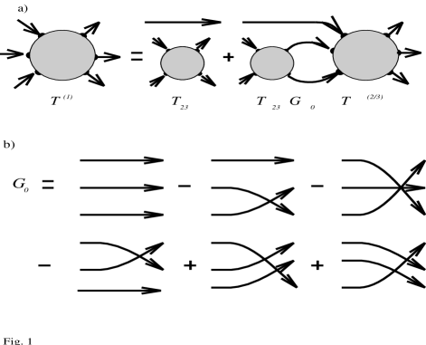
where subscripts $[p..]$ and $[h..]$ refer to particle and hole states respectively. The first line corresponds the 3-particle channel which is dominant in Fermi-systems interacting via short-range forces, and to which we shall restrict ourselves. The Faddeev decompositon, eq. (71), and five exchange diagrams for this case are shown in Fig. 1.

The signs of the exchange diagrams are given by $(-1)^{n}$, where $n$ is the number of the line intersections in the diagram. The respective exchange terms for the remainder of the diagrams are obtained by interchanging the time-direction of lines.

A Fourier transformation in eq. (71) with respect to the relative times leads to the 3-particle ${\cal T}$-matrix

$$\langle\mbox{\boldmath$k$}_{23},\mbox{\boldmath$q$}_{1}|{\cal T}^{R\,(1)}(K)|\mbox{\boldmath$k$}_{23}^{\prime},\mbox{\boldmath$q$}_{1}^{\prime}\rangle = \langle\mbox{\boldmath$k$}_{23},\mbox{\boldmath$q$}_{1}|{\cal T}^{R}_{23}(K)|\mbox{\boldmath$k$}_{23}^{\prime},\mbox{\boldmath$q$}_{1}^{\prime}\rangle$$ (82)

$$+ \int\Bigl{\{}\Big{\langle}\frac{\mbox{\boldmath$k$}_{23}}{2}-\frac{3\mbox{\boldmath$q$}_{1}}{4},-\mbox{\boldmath$k$}_{23}-\frac{\mbox{\boldmath$q$}_{1}}{2}\Big{|}{\cal T}^{R\,(2)}(K)|\mbox{\boldmath$k$}_{13}^{\prime\prime},\mbox{\boldmath$q$}_{2}^{\prime\prime}\rangle$$ (83)

$$+ \Big{\langle}\frac{\mbox{\boldmath$k$}_{23}}{2}+\frac{3\mbox{\boldmath$q$}_{1}}{4},-\mbox{\boldmath$k$}_{23}+\frac{\mbox{\boldmath$q$}_{1}}{2}\Big{|}{\cal T}^{R\,(3)}(K)|\mbox{\boldmath$k$}_{13}^{\prime\prime},\mbox{\boldmath$q$}_{2}^{\prime\prime}\rangle\Bigl{\}}$$ (84)

$$\times \frac{Q(K^{\prime},k_{13}^{\prime\prime},q_{2}^{\prime\prime})\delta(\mbox{\boldmath$K$}-\mbox{\boldmath$K$}^{\prime})}{\Omega-\Omega^{\prime}+i\eta}$$ (85)

$$\times \Big{\langle}\frac{\mbox{\boldmath$k$}^{\prime\prime}_{13}}{2}-\frac{3\mbox{\boldmath$q$}^{\prime\prime}_{2}}{4},-\mbox{\boldmath$k$}^{\prime\prime}_{13}-\frac{\mbox{\boldmath$q$}_{2}^{\prime\prime}}{3}\Big{|}{\cal T}^{R}_{23}(K)|\mbox{\boldmath$k$}_{23}^{\prime},\mbox{\boldmath$q$}_{1}^{\prime}\rangle$$ (86)

$$\times \,d\omega_{13}^{\prime\prime}d\mbox{\boldmath$k$}_{13}^{\prime\prime}d\nu_{2}^{\prime\prime}d\mbox{\boldmath$q$}_{2}^{\prime\prime}d\Omega^{\prime}d\mbox{\boldmath$K$}^{\prime},$$ (87)

with

$$Q(K,k_{13},q_{2}) = \Bigl{\{}G^{>}\left(K/3+k_{13}+q_{2}/2\right)G^{>}\left(K/3-k_{13}+q_{2}/2\right)G^{>}\left(K/3-q_{2}\right)$$ (88)

$$- G^{<}\left(K/3+k_{13}+q_{2}/2\right)G^{<}\left(K/3-k_{13}+q_{2}/2\right)G^{<}\left(K/3-q_{2}\right)\Bigr{\}},$$ (89)

and four-vector notation $K=(\Omega,\mbox{\boldmath$K$})$, $k=(\omega,\mbox{\boldmath$k$})$, $q=(\nu,\mbox{\boldmath$q$})$. The momentum representation of equations for ${\cal T}^{(2)}$ and ${\cal T}^{(3)}$ follows from (82) by permutations of (Greek) indexes $1\leftrightarrow 2$ and $1\leftrightarrow 3$.

FIG. 1.: a) The three-body amplitudes in the 3-particle channel after Faddeev rearrangement; only one of the terms of the type ${\cal T}^{(\alpha)}$ appearing on the right hand side is shown. b) The direct and five exchange three particle propagators. The diagrams for processes involving hole propagations are obtained by interchanging the direction of the lines.

To the lowest order in the expansion of the off-diagonal single-particle Green’s function we find the QP result

$$\langle\mbox{\boldmath$k$}_{23},\mbox{\boldmath$q$}_{1}|{\cal T}^{R\,(1)}(K)|\mbox{\boldmath$k$}_{23}^{\prime},\mbox{\boldmath$q$}_{1}^{\prime}\rangle = \langle\mbox{\boldmath$k$}_{23},\mbox{\boldmath$q$}_{1}|{\cal T}^{R}_{23}(K)|\mbox{\boldmath$k$}_{23}^{\prime},\mbox{\boldmath$q$}_{1}^{\prime}\rangle$$ (90)

$$+ \int\Bigl{\{}\Big{\langle}\frac{\mbox{\boldmath$k$}_{23}}{2}-\frac{3\mbox{\boldmath$q$}_{1}}{4},-\mbox{\boldmath$k$}_{23}-\frac{\mbox{\boldmath$q$}_{1}}{2}\Big{|}{\cal T}^{R\,(2)}(K)|\mbox{\boldmath$k$}_{13}^{\prime\prime},\mbox{\boldmath$q$}_{2}^{\prime\prime}\rangle$$ (91)

$$+ \Big{\langle}\frac{\mbox{\boldmath$k$}_{23}}{2}+\frac{3\mbox{\boldmath$q$}_{1}}{4},-\mbox{\boldmath$k$}_{23}+\frac{\mbox{\boldmath$q$}_{1}}{2}\Big{|}{\cal T}^{R\,(3)}(K)|\mbox{\boldmath$k$}_{13}^{\prime\prime},\mbox{\boldmath$q$}_{2}^{\prime\prime}\rangle\Bigl{\}}\,Q(\mbox{\boldmath$K$},\mbox{\boldmath$k$}_{13}^{\prime\prime},\mbox{\boldmath$q$}_{2}^{\prime\prime})$$ (92)

$$\times \frac{\Big{\langle}\frac{\mbox{\boldmath$k$}^{\prime\prime}_{13}}{2}-\frac{3\mbox{\boldmath$q$}^{\prime\prime}_{2}}{4},-\mbox{\boldmath$k$}^{\prime\prime}_{13}-\frac{\mbox{\boldmath$q$}_{2}^{\prime\prime}}{3}\Big{|}{\cal T}^{R}_{23}(K)|\mbox{\boldmath$q$}_{23}^{\prime},\mbox{\boldmath$q$}_{1}^{\prime}\rangle}{\Omega-\epsilon_{\vec{K}/3+\vec{k}_{13}^{\prime\prime}+\vec{q}_{2}^{\prime\prime}/2}-\epsilon_{\vec{K}/3-\vec{k}_{13}^{\prime\prime}+\vec{q}_{2}^{\prime\prime}/2}-\epsilon_{\vec{K}/3-\vec{q}_{2}^{\prime\prime}}+i\eta}d\mbox{\boldmath$k$}_{13}^{\prime\prime}d\mbox{\boldmath$q$}_{2}^{\prime\prime},$$ (93)

with

$$Q(\mbox{\boldmath$K$},\mbox{\boldmath$k$}_{13},\mbox{\boldmath$q$}_{2}) = 1-f\left(\mbox{\boldmath$K$}/3+\mbox{\boldmath$k$}_{13}+\mbox{\boldmath$q$}_{2}/2\right)-f\left(\mbox{\boldmath$K$}/3-\mbox{\boldmath$k$}_{13}+\mbox{\boldmath$q$}_{2}/2\right)-f\left(\mbox{\boldmath$K$}/3-\mbox{\boldmath$q$}_{2}\right)$$ (95)

$$- f\left(\mbox{\boldmath$K$}/3+\mbox{\boldmath$k$}_{13}+\mbox{\boldmath$q$}_{2}/2\right)f\left(\mbox{\boldmath$K$}/3-\mbox{\boldmath$k$}_{13}+\mbox{\boldmath$q$}_{2}/2\right)$$ (96)

$$- f\left(\mbox{\boldmath$K$}/3+\mbox{\boldmath$k$}_{13}+\mbox{\boldmath$q$}_{2}/2\right)f\left(\mbox{\boldmath$K$}/3-\mbox{\boldmath$q$}_{2}\right)$$ (97)

$$- f\left(\mbox{\boldmath$K$}/3-\mbox{\boldmath$k$}_{13}+\mbox{\boldmath$q$}_{2}/2\right)f\left(\mbox{\boldmath$K$}/3-\mbox{\boldmath$q$}_{2}\right).$$ (98)

Equations (82) and (90) provide the Faddeev amplitudes appropriate at finite densities and temperatures. The medium effects enter these equations in two ways: (i) the renormalization of the single particle spectrum in the resolvent of eq. (82), and (ii) statistically occupied intermediate state propagation. The first line of eq. (95) is the Pauli-blocking of intermediate propagation of three particles and is the dominant term in the dilute limit. The remainder of the terms, in the same limit, tend to Bose-enhance the intermediate propagation, which can be seen from the equilibrium identity $f(\omega_{1})f(\omega_{2})=g(\omega_{1}+\omega_{2})\left[1-f(\omega_{1})-f(\omega_{2})\right]$, where $f$ and $g$ are the Fermi and Bose distribution functions. Inclusion of the next to leading order terms in the powers of $\gamma$ can be constructed in a manner similar to the two-body case, however would lead to implicite inclusion of four body correlations, which are beyond of the scope of this paper. In the limit $Q\to 1$ these equations reduce to the original Faddeev equations (of course with the particle spectrum $\epsilon=p^{2}/2m$).

IV Scattering Integrals

A Transport Vertex

The self-energies in the matrix formulation of nonequilibrium theory have a structure topologically identical to the equilibrium case. We shall adopt the cluster expansion for the self-energy matrix  [41, 42] and, consistent with the discussion above, truncate it at the three-body level:

$${\bf\Sigma}_{12}={\bf T}_{1234}\otimes{\bf G}_{43^{+}}+{\mathchoice{{\hbox{\boldmath$\displaystyle\cal T$}}}{{\hbox{\boldmath$\textstyle\cal T$}}}{{\hbox{\boldmath$\scriptstyle\cal T$}}}{{\hbox{\boldmath$\scriptscriptstyle\cal T$}}}}_{165432}\otimes{\bf G}_{43^{+}}\,{\bf G}_{65^{+}},$$ (99)

where $+$ means an infinitesimal later time point. The non-diagonal elements of the matrix equation provide the collision rates on the right hand side of the kinetic equations. In the mixed representation one finds

$$\Sigma^{<}(p_{1}) = -i\sum_{p_{2}}\langle{(\mathchoice{{\hbox{\boldmath$\displaystyle p$}}}{{\hbox{\boldmath$\textstyle p$}}}{{\hbox{\boldmath$\scriptstyle p$}}}{{\hbox{\boldmath$\scriptscriptstyle p$}}}_{1}-\mathchoice{{\hbox{\boldmath$\displaystyle p$}}}{{\hbox{\boldmath$\textstyle p$}}}{{\hbox{\boldmath$\scriptstyle p$}}}{{\hbox{\boldmath$\scriptscriptstyle p$}}}_{2})/}{2}|T^{<}(p_{1}+p_{2},)|{(\mathchoice{{\hbox{\boldmath$\displaystyle p$}}}{{\hbox{\boldmath$\textstyle p$}}}{{\hbox{\boldmath$\scriptstyle p$}}}{{\hbox{\boldmath$\scriptscriptstyle p$}}}_{1}-\mathchoice{{\hbox{\boldmath$\displaystyle p$}}}{{\hbox{\boldmath$\textstyle p$}}}{{\hbox{\boldmath$\scriptstyle p$}}}{{\hbox{\boldmath$\scriptscriptstyle p$}}}_{2})/}{2}\rangle\,G^{>}(p_{2},)$$ (100)

$$+ \sum_{p_{2},p_{3}}\Bigl{[}\langle\mbox{\boldmath$k$}_{23},\mbox{\boldmath$q$}_{1}|{\cal T}^{(1)\,<}(K)|\mbox{\boldmath$k$}_{23},\mbox{\boldmath$q$}_{1}\rangle\,+\langle\mbox{\boldmath$k$}_{13},\mbox{\boldmath$q$}_{2}|{\cal T}^{(2)\,<}(K)|\mbox{\boldmath$k$}_{13},\mbox{\boldmath$q$}_{2}\rangle\,$$ (101)

$$+ \langle\mbox{\boldmath$k$}_{12},\mbox{\boldmath$q$}_{3}|{\cal T}^{(3)\,<}(K)|\mbox{\boldmath$k$}_{12},\mbox{\boldmath$q$}_{3}\rangle\,\Bigr{]}G^{>}(p_{2})\,G^{>}(p_{3}).$$ (102)

The expression for $\Sigma^{>}$ follows by simultaneous interchange of $<$ and $>$ signs. The Jacobi momenta in the three-body ${\cal T}$-matrix are related to the arguments of the self-energy and the Green’s functions via the relations (77). Equation (100) does not imply the usual form of the transition probability as a square of the transition amplitude times the statistical factors (i.e. Fermi Golden Rule). For the purpose of recovering this form one may use the non-equilibrium optical theorem

$$\langle\mathchoice{{\hbox{\boldmath$\displaystyle p$}}}{{\hbox{\boldmath$\textstyle p$}}}{{\hbox{\boldmath$\scriptstyle p$}}}{{\hbox{\boldmath$\scriptscriptstyle p$}}}_{1}|T^{<}(P)|\mathchoice{{\hbox{\boldmath$\displaystyle p$}}}{{\hbox{\boldmath$\textstyle p$}}}{{\hbox{\boldmath$\scriptstyle p$}}}{{\hbox{\boldmath$\scriptscriptstyle p$}}}_{2}\rangle = -i\sum_{p_{3}\,p_{4}}\langle\mathchoice{{\hbox{\boldmath$\displaystyle p$}}}{{\hbox{\boldmath$\textstyle p$}}}{{\hbox{\boldmath$\scriptstyle p$}}}{{\hbox{\boldmath$\scriptscriptstyle p$}}}_{1}|T^{R}(P)|\frac{\mathchoice{{\hbox{\boldmath$\displaystyle p$}}}{{\hbox{\boldmath$\textstyle p$}}}{{\hbox{\boldmath$\scriptstyle p$}}}{{\hbox{\boldmath$\scriptscriptstyle p$}}}_{3}-\mathchoice{{\hbox{\boldmath$\displaystyle p$}}}{{\hbox{\boldmath$\textstyle p$}}}{{\hbox{\boldmath$\scriptstyle p$}}}{{\hbox{\boldmath$\scriptscriptstyle p$}}}_{4}}{2}\Big{\rangle}~{}G^{<}(p_{3})\,G^{<}(p_{4})\Big{\langle}\frac{\mathchoice{{\hbox{\boldmath$\displaystyle p$}}}{{\hbox{\boldmath$\textstyle p$}}}{{\hbox{\boldmath$\scriptstyle p$}}}{{\hbox{\boldmath$\scriptscriptstyle p$}}}_{3}-\mathchoice{{\hbox{\boldmath$\displaystyle p$}}}{{\hbox{\boldmath$\textstyle p$}}}{{\hbox{\boldmath$\scriptstyle p$}}}{{\hbox{\boldmath$\scriptscriptstyle p$}}}_{4}}{2}|T^{A}(P)|\mathchoice{{\hbox{\boldmath$\displaystyle p$}}}{{\hbox{\boldmath$\textstyle p$}}}{{\hbox{\boldmath$\scriptstyle p$}}}{{\hbox{\boldmath$\scriptscriptstyle p$}}}_{2}\rangle$$ (103)

$$\times (2\pi)^{4}\,\delta^{4}(P-p_{3}-p_{4}),$$ (104)

$$\langle\mbox{\boldmath$k$}_{23},\mbox{\boldmath$q$}_{1}|{\cal T}^{<}(K)|\mbox{\boldmath$k$}_{23}^{\prime},\mbox{\boldmath$q$}_{1}^{\prime}\rangle = \sum_{\alpha,\beta}\sum_{p_{4},p_{5},p_{6}}\langle\mbox{\boldmath$k$}_{23},\mbox{\boldmath$q$}_{1}|{\cal T}^{(\alpha)\,R}(K)|\mbox{\boldmath$k$}_{45},\mbox{\boldmath$q$}_{6}\rangle\,G^{<}(p_{4})\,G^{<}(p_{5})\,G^{<}(p_{6})$$ (105)

$$\times \langle\mbox{\boldmath$k$}_{45},\mbox{\boldmath$q$}_{6}|{\cal T}^{(\beta)\,A}(K)|\mbox{\boldmath$k$}_{23}^{\prime},\mbox{\boldmath$q$}_{1}^{\prime}\rangle(2\pi)^{4}\,\delta^{4}(K-p_{4}-p_{5}-p_{6}).$$ (106)

Combination of the equations (100),(103), and (105) yields the usual form of the quantum Boltzmann collision integrals with scattering probabilities defined as

$$\langle\mathchoice{{\hbox{\boldmath$\displaystyle p$}}}{{\hbox{\boldmath$\textstyle p$}}}{{\hbox{\boldmath$\scriptstyle p$}}}{{\hbox{\boldmath$\scriptscriptstyle p$}}}_{1},\mathchoice{{\hbox{\boldmath$\displaystyle p$}}}{{\hbox{\boldmath$\textstyle p$}}}{{\hbox{\boldmath$\scriptstyle p$}}}{{\hbox{\boldmath$\scriptscriptstyle p$}}}_{2}|W|\mathchoice{{\hbox{\boldmath$\displaystyle p$}}}{{\hbox{\boldmath$\textstyle p$}}}{{\hbox{\boldmath$\scriptstyle p$}}}{{\hbox{\boldmath$\scriptscriptstyle p$}}}_{3},\mathchoice{{\hbox{\boldmath$\displaystyle p$}}}{{\hbox{\boldmath$\textstyle p$}}}{{\hbox{\boldmath$\scriptstyle p$}}}{{\hbox{\boldmath$\scriptscriptstyle p$}}}_{4}\rangle = \langle(\mathchoice{{\hbox{\boldmath$\displaystyle p$}}}{{\hbox{\boldmath$\textstyle p$}}}{{\hbox{\boldmath$\scriptstyle p$}}}{{\hbox{\boldmath$\scriptscriptstyle p$}}}_{1}-\mathchoice{{\hbox{\boldmath$\displaystyle p$}}}{{\hbox{\boldmath$\textstyle p$}}}{{\hbox{\boldmath$\scriptstyle p$}}}{{\hbox{\boldmath$\scriptscriptstyle p$}}}_{2})/2|T^{R}(P)|{(\mathchoice{{\hbox{\boldmath$\displaystyle p$}}}{{\hbox{\boldmath$\textstyle p$}}}{{\hbox{\boldmath$\scriptstyle p$}}}{{\hbox{\boldmath$\scriptscriptstyle p$}}}_{3}-\mathchoice{{\hbox{\boldmath$\displaystyle p$}}}{{\hbox{\boldmath$\textstyle p$}}}{{\hbox{\boldmath$\scriptstyle p$}}}{{\hbox{\boldmath$\scriptscriptstyle p$}}}_{4})/}{2}\rangle\langle{(\mathchoice{{\hbox{\boldmath$\displaystyle p$}}}{{\hbox{\boldmath$\textstyle p$}}}{{\hbox{\boldmath$\scriptstyle p$}}}{{\hbox{\boldmath$\scriptscriptstyle p$}}}_{3}-\mathchoice{{\hbox{\boldmath$\displaystyle p$}}}{{\hbox{\boldmath$\textstyle p$}}}{{\hbox{\boldmath$\scriptstyle p$}}}{{\hbox{\boldmath$\scriptscriptstyle p$}}}_{4})}/{2}|T^{A}(P)|(\mathchoice{{\hbox{\boldmath$\displaystyle p$}}}{{\hbox{\boldmath$\textstyle p$}}}{{\hbox{\boldmath$\scriptstyle p$}}}{{\hbox{\boldmath$\scriptscriptstyle p$}}}_{1}-\mathchoice{{\hbox{\boldmath$\displaystyle p$}}}{{\hbox{\boldmath$\textstyle p$}}}{{\hbox{\boldmath$\scriptstyle p$}}}{{\hbox{\boldmath$\scriptscriptstyle p$}}}_{2})/2\rangle$$ (107)

$$\times \delta^{3}(\mathchoice{{\hbox{\boldmath$\displaystyle p$}}}{{\hbox{\boldmath$\textstyle p$}}}{{\hbox{\boldmath$\scriptstyle p$}}}{{\hbox{\boldmath$\scriptscriptstyle p$}}}_{1}+\mathchoice{{\hbox{\boldmath$\displaystyle p$}}}{{\hbox{\boldmath$\textstyle p$}}}{{\hbox{\boldmath$\scriptstyle p$}}}{{\hbox{\boldmath$\scriptscriptstyle p$}}}_{2}-\mathchoice{{\hbox{\boldmath$\displaystyle p$}}}{{\hbox{\boldmath$\textstyle p$}}}{{\hbox{\boldmath$\scriptstyle p$}}}{{\hbox{\boldmath$\scriptscriptstyle p$}}}_{3}-\mathchoice{{\hbox{\boldmath$\displaystyle p$}}}{{\hbox{\boldmath$\textstyle p$}}}{{\hbox{\boldmath$\scriptstyle p$}}}{{\hbox{\boldmath$\scriptscriptstyle p$}}}_{4})$$ (108)

$$\langle\mathchoice{{\hbox{\boldmath$\displaystyle p$}}}{{\hbox{\boldmath$\textstyle p$}}}{{\hbox{\boldmath$\scriptstyle p$}}}{{\hbox{\boldmath$\scriptscriptstyle p$}}}_{1},\mathchoice{{\hbox{\boldmath$\displaystyle p$}}}{{\hbox{\boldmath$\textstyle p$}}}{{\hbox{\boldmath$\scriptstyle p$}}}{{\hbox{\boldmath$\scriptscriptstyle p$}}}_{2},\mathchoice{{\hbox{\boldmath$\displaystyle p$}}}{{\hbox{\boldmath$\textstyle p$}}}{{\hbox{\boldmath$\scriptstyle p$}}}{{\hbox{\boldmath$\scriptscriptstyle p$}}}_{3}|{\cal W}|\mathchoice{{\hbox{\boldmath$\displaystyle p$}}}{{\hbox{\boldmath$\textstyle p$}}}{{\hbox{\boldmath$\scriptstyle p$}}}{{\hbox{\boldmath$\scriptscriptstyle p$}}}_{4},\mathchoice{{\hbox{\boldmath$\displaystyle p$}}}{{\hbox{\boldmath$\textstyle p$}}}{{\hbox{\boldmath$\scriptstyle p$}}}{{\hbox{\boldmath$\scriptscriptstyle p$}}}_{5},\mathchoice{{\hbox{\boldmath$\displaystyle p$}}}{{\hbox{\boldmath$\textstyle p$}}}{{\hbox{\boldmath$\scriptstyle p$}}}{{\hbox{\boldmath$\scriptscriptstyle p$}}}_{6}\rangle = \sum_{\alpha,\beta}\langle\mbox{\boldmath$k$}_{23},\mbox{\boldmath$q$}_{1}|{\cal T}^{(\alpha)\,R}(K)|\mbox{\boldmath$k$}_{45},\mbox{\boldmath$q$}_{6}\rangle\,\langle\mbox{\boldmath$k$}_{45},\mbox{\boldmath$q$}_{6}|{\cal T}^{(\beta)\,A}(K)|\mbox{\boldmath$k$}_{23},\mbox{\boldmath$q$}_{1}\rangle$$ (109)

$$\times (2\pi)^{3}\,\delta^{3}(\mathchoice{{\hbox{\boldmath$\displaystyle p$}}}{{\hbox{\boldmath$\textstyle p$}}}{{\hbox{\boldmath$\scriptstyle p$}}}{{\hbox{\boldmath$\scriptscriptstyle p$}}}_{1}+\mathchoice{{\hbox{\boldmath$\displaystyle p$}}}{{\hbox{\boldmath$\textstyle p$}}}{{\hbox{\boldmath$\scriptstyle p$}}}{{\hbox{\boldmath$\scriptscriptstyle p$}}}_{2}+\mathchoice{{\hbox{\boldmath$\displaystyle p$}}}{{\hbox{\boldmath$\textstyle p$}}}{{\hbox{\boldmath$\scriptstyle p$}}}{{\hbox{\boldmath$\scriptscriptstyle p$}}}_{3}-\mathchoice{{\hbox{\boldmath$\displaystyle p$}}}{{\hbox{\boldmath$\textstyle p$}}}{{\hbox{\boldmath$\scriptstyle p$}}}{{\hbox{\boldmath$\scriptscriptstyle p$}}}_{4}-\mathchoice{{\hbox{\boldmath$\displaystyle p$}}}{{\hbox{\boldmath$\textstyle p$}}}{{\hbox{\boldmath$\scriptstyle p$}}}{{\hbox{\boldmath$\scriptscriptstyle p$}}}_{5}-\mathchoice{{\hbox{\boldmath$\displaystyle p$}}}{{\hbox{\boldmath$\textstyle p$}}}{{\hbox{\boldmath$\scriptstyle p$}}}{{\hbox{\boldmath$\scriptscriptstyle p$}}}_{6}),$$ (110)

where it is understood that the Jacobi momenta in the three-body transition probability $\cal W$ should be expressed through the momenta $p_{i}$, $i=1...6$, via the relations (77).

The diagonal elements of the matrix equation (99) provide the solution of the integral Dyson equation and thus, the renormalization of the single particle spectrum. Apart from the details (which can be deduced along the lines of the previous discussion, see Section 1 E), let us note that (i) in the next-to-leading order approximation to the spectral function the mean-field due to the excitations occupying off-mass-shell states contributes to the the real part of the self-energy; (ii) an additional contribution to the self-energy comes from the off-mass-shell $T$-matrices folded by the on-shell quasiparticle distribution - a contribution which is missing in the usual Brueckner theory; (iii) the three-body processes contribute to the energy shift in the single particle spectrum via the second term of the cluster expansion.

B Virial expansion of collision integrals

The general form of the collision integral can be arranged in the form of virial corrections in much the same manner as the diagrams of scattering theory (Section 1 C). In principle, in the next-to-leading order approximation this collision integral can be separated into the quasiparticle and correlated contributions in two different ways, corresponding to the partition in the pole and off-pole terms and in the powers of $\gamma$. The latter partition is physically more appealing, since it involves the coupling between the kinetic equations for on-shell quasipaticles and off-shell excitations. This decomposition for the two-body scattering integral contains five terms

$$I(\mathchoice{{\hbox{\boldmath$\displaystyle p$}}}{{\hbox{\boldmath$\textstyle p$}}}{{\hbox{\boldmath$\scriptstyle p$}}}{{\hbox{\boldmath$\scriptscriptstyle p$}}},x)=I^{(0)}(\mathchoice{{\hbox{\boldmath$\displaystyle p$}}}{{\hbox{\boldmath$\textstyle p$}}}{{\hbox{\boldmath$\scriptstyle p$}}}{{\hbox{\boldmath$\scriptscriptstyle p$}}},x)+I^{(1)}(\mathchoice{{\hbox{\boldmath$\displaystyle p$}}}{{\hbox{\boldmath$\textstyle p$}}}{{\hbox{\boldmath$\scriptstyle p$}}}{{\hbox{\boldmath$\scriptscriptstyle p$}}},x)+I^{(2)}(\mathchoice{{\hbox{\boldmath$\displaystyle p$}}}{{\hbox{\boldmath$\textstyle p$}}}{{\hbox{\boldmath$\scriptstyle p$}}}{{\hbox{\boldmath$\scriptscriptstyle p$}}},x)+I^{(3)}(\mathchoice{{\hbox{\boldmath$\displaystyle p$}}}{{\hbox{\boldmath$\textstyle p$}}}{{\hbox{\boldmath$\scriptstyle p$}}}{{\hbox{\boldmath$\scriptscriptstyle p$}}},x)+I^{(4)}(\mathchoice{{\hbox{\boldmath$\displaystyle p$}}}{{\hbox{\boldmath$\textstyle p$}}}{{\hbox{\boldmath$\scriptstyle p$}}}{{\hbox{\boldmath$\scriptscriptstyle p$}}},x);$$ (111)

a similar decomposition emerges for the three-body collision integral ${\cal I}$. The first terms in the decomposition i.e. the scattering integrals for the quasiparticles,

$$I^{(0)}(\mathchoice{{\hbox{\boldmath$\displaystyle p$}}}{{\hbox{\boldmath$\textstyle p$}}}{{\hbox{\boldmath$\scriptstyle p$}}}{{\hbox{\boldmath$\scriptscriptstyle p$}}}_{1}) = \sum_{\bf p_{2}p_{3}p_{4}}\langle\mathchoice{{\hbox{\boldmath$\displaystyle p$}}}{{\hbox{\boldmath$\textstyle p$}}}{{\hbox{\boldmath$\scriptstyle p$}}}{{\hbox{\boldmath$\scriptscriptstyle p$}}}_{1},\mathchoice{{\hbox{\boldmath$\displaystyle p$}}}{{\hbox{\boldmath$\textstyle p$}}}{{\hbox{\boldmath$\scriptstyle p$}}}{{\hbox{\boldmath$\scriptscriptstyle p$}}}_{2}|W|\mathchoice{{\hbox{\boldmath$\displaystyle p$}}}{{\hbox{\boldmath$\textstyle p$}}}{{\hbox{\boldmath$\scriptstyle p$}}}{{\hbox{\boldmath$\scriptscriptstyle p$}}}_{3},\mathchoice{{\hbox{\boldmath$\displaystyle p$}}}{{\hbox{\boldmath$\textstyle p$}}}{{\hbox{\boldmath$\scriptstyle p$}}}{{\hbox{\boldmath$\scriptscriptstyle p$}}}_{4}\rangle\delta(\varepsilon_{p_{1}}+\varepsilon_{p_{2}}-\varepsilon_{p_{3}}-\varepsilon_{p_{4}})$$ (112)

$$\times \left\{f(\mathchoice{{\hbox{\boldmath$\displaystyle p$}}}{{\hbox{\boldmath$\textstyle p$}}}{{\hbox{\boldmath$\scriptstyle p$}}}{{\hbox{\boldmath$\scriptscriptstyle p$}}}_{1})\,f(\mathchoice{{\hbox{\boldmath$\displaystyle p$}}}{{\hbox{\boldmath$\textstyle p$}}}{{\hbox{\boldmath$\scriptstyle p$}}}{{\hbox{\boldmath$\scriptscriptstyle p$}}}_{2})[1-f(\mathchoice{{\hbox{\boldmath$\displaystyle p$}}}{{\hbox{\boldmath$\textstyle p$}}}{{\hbox{\boldmath$\scriptstyle p$}}}{{\hbox{\boldmath$\scriptscriptstyle p$}}}_{3})][1-f(\mathchoice{{\hbox{\boldmath$\displaystyle p$}}}{{\hbox{\boldmath$\textstyle p$}}}{{\hbox{\boldmath$\scriptstyle p$}}}{{\hbox{\boldmath$\scriptscriptstyle p$}}}_{4})]-[1-f(\mathchoice{{\hbox{\boldmath$\displaystyle p$}}}{{\hbox{\boldmath$\textstyle p$}}}{{\hbox{\boldmath$\scriptstyle p$}}}{{\hbox{\boldmath$\scriptscriptstyle p$}}}_{1})][1-f(\mathchoice{{\hbox{\boldmath$\displaystyle p$}}}{{\hbox{\boldmath$\textstyle p$}}}{{\hbox{\boldmath$\scriptstyle p$}}}{{\hbox{\boldmath$\scriptscriptstyle p$}}}_{2})]f(\mathchoice{{\hbox{\boldmath$\displaystyle p$}}}{{\hbox{\boldmath$\textstyle p$}}}{{\hbox{\boldmath$\scriptstyle p$}}}{{\hbox{\boldmath$\scriptscriptstyle p$}}}_{3})\,f(\mathchoice{{\hbox{\boldmath$\displaystyle p$}}}{{\hbox{\boldmath$\textstyle p$}}}{{\hbox{\boldmath$\scriptstyle p$}}}{{\hbox{\boldmath$\scriptscriptstyle p$}}}_{4})\right\},$$ (113)

$${\cal I}^{(0)}(\mathchoice{{\hbox{\boldmath$\displaystyle p$}}}{{\hbox{\boldmath$\textstyle p$}}}{{\hbox{\boldmath$\scriptstyle p$}}}{{\hbox{\boldmath$\scriptscriptstyle p$}}}_{1}) = \sum_{\bf p_{2}p_{3}p_{4}p_{5}p_{6}}\langle\mathchoice{{\hbox{\boldmath$\displaystyle p$}}}{{\hbox{\boldmath$\textstyle p$}}}{{\hbox{\boldmath$\scriptstyle p$}}}{{\hbox{\boldmath$\scriptscriptstyle p$}}}_{1},\mathchoice{{\hbox{\boldmath$\displaystyle p$}}}{{\hbox{\boldmath$\textstyle p$}}}{{\hbox{\boldmath$\scriptstyle p$}}}{{\hbox{\boldmath$\scriptscriptstyle p$}}}_{2},\mathchoice{{\hbox{\boldmath$\displaystyle p$}}}{{\hbox{\boldmath$\textstyle p$}}}{{\hbox{\boldmath$\scriptstyle p$}}}{{\hbox{\boldmath$\scriptscriptstyle p$}}}_{3}|W|\mathchoice{{\hbox{\boldmath$\displaystyle p$}}}{{\hbox{\boldmath$\textstyle p$}}}{{\hbox{\boldmath$\scriptstyle p$}}}{{\hbox{\boldmath$\scriptscriptstyle p$}}}_{4},\mathchoice{{\hbox{\boldmath$\displaystyle p$}}}{{\hbox{\boldmath$\textstyle p$}}}{{\hbox{\boldmath$\scriptstyle p$}}}{{\hbox{\boldmath$\scriptscriptstyle p$}}}_{5},\mathchoice{{\hbox{\boldmath$\displaystyle p$}}}{{\hbox{\boldmath$\textstyle p$}}}{{\hbox{\boldmath$\scriptstyle p$}}}{{\hbox{\boldmath$\scriptscriptstyle p$}}}_{6}\rangle\delta(\varepsilon_{p_{1}}+\varepsilon_{p_{2}}+\varepsilon_{p_{3}}-\varepsilon_{p_{4}}-\varepsilon_{5}-\varepsilon_{6})$$ (114)

$$\times \Big{\{}f(\mathchoice{{\hbox{\boldmath$\displaystyle p$}}}{{\hbox{\boldmath$\textstyle p$}}}{{\hbox{\boldmath$\scriptstyle p$}}}{{\hbox{\boldmath$\scriptscriptstyle p$}}}_{1})\,f(\mathchoice{{\hbox{\boldmath$\displaystyle p$}}}{{\hbox{\boldmath$\textstyle p$}}}{{\hbox{\boldmath$\scriptstyle p$}}}{{\hbox{\boldmath$\scriptscriptstyle p$}}}_{2})\,f(\mathchoice{{\hbox{\boldmath$\displaystyle p$}}}{{\hbox{\boldmath$\textstyle p$}}}{{\hbox{\boldmath$\scriptstyle p$}}}{{\hbox{\boldmath$\scriptscriptstyle p$}}}_{3})[1-f(\mathchoice{{\hbox{\boldmath$\displaystyle p$}}}{{\hbox{\boldmath$\textstyle p$}}}{{\hbox{\boldmath$\scriptstyle p$}}}{{\hbox{\boldmath$\scriptscriptstyle p$}}}_{4})][1-f(\mathchoice{{\hbox{\boldmath$\displaystyle p$}}}{{\hbox{\boldmath$\textstyle p$}}}{{\hbox{\boldmath$\scriptstyle p$}}}{{\hbox{\boldmath$\scriptscriptstyle p$}}}_{5})][1-f(\mathchoice{{\hbox{\boldmath$\displaystyle p$}}}{{\hbox{\boldmath$\textstyle p$}}}{{\hbox{\boldmath$\scriptstyle p$}}}{{\hbox{\boldmath$\scriptscriptstyle p$}}}_{6})]$$ (115)

$$- [1-f(\mathchoice{{\hbox{\boldmath$\displaystyle p$}}}{{\hbox{\boldmath$\textstyle p$}}}{{\hbox{\boldmath$\scriptstyle p$}}}{{\hbox{\boldmath$\scriptscriptstyle p$}}}_{1})][1-f(\mathchoice{{\hbox{\boldmath$\displaystyle p$}}}{{\hbox{\boldmath$\textstyle p$}}}{{\hbox{\boldmath$\scriptstyle p$}}}{{\hbox{\boldmath$\scriptscriptstyle p$}}}_{2})][1-f(\mathchoice{{\hbox{\boldmath$\displaystyle p$}}}{{\hbox{\boldmath$\textstyle p$}}}{{\hbox{\boldmath$\scriptstyle p$}}}{{\hbox{\boldmath$\scriptscriptstyle p$}}}_{3})]f(\mathchoice{{\hbox{\boldmath$\displaystyle p$}}}{{\hbox{\boldmath$\textstyle p$}}}{{\hbox{\boldmath$\scriptstyle p$}}}{{\hbox{\boldmath$\scriptscriptstyle p$}}}_{4})\,f(\mathchoice{{\hbox{\boldmath$\displaystyle p$}}}{{\hbox{\boldmath$\textstyle p$}}}{{\hbox{\boldmath$\scriptstyle p$}}}{{\hbox{\boldmath$\scriptscriptstyle p$}}}_{5})\,f(\mathchoice{{\hbox{\boldmath$\displaystyle p$}}}{{\hbox{\boldmath$\textstyle p$}}}{{\hbox{\boldmath$\scriptstyle p$}}}{{\hbox{\boldmath$\scriptscriptstyle p$}}}_{6})\Big{\}},$$ (116)

describe the scattering of two/three incoming uncorrelated quasiparticles into uncorrelated outgoing states. Note that the retarded amplitudes in the collision probabilities include, apart from the usual Pauli-blocking due to the uncorrelated quasiparticles, the off-shell intermediate propagation effects and the phase space occupation due to the off-shell excitations in the medium.

The remaining collision integrals describe scattering processes where one of the incoming or outgoing excitations is in a correlated state. (The upper index labels the correlated particle). Note, however, that the processes involving correlated states implicitly contain at least an extra quasiparticle. The terms of higher than zeroth order in the three particle collision integrals, therefore, involve processes with four or larger number of quasiparticles and can be ignored. As to the two-body case, the result for the second term of the decomposition reads

$$I^{(1)}(\mathchoice{{\hbox{\boldmath$\displaystyle p$}}}{{\hbox{\boldmath$\textstyle p$}}}{{\hbox{\boldmath$\scriptstyle p$}}}{{\hbox{\boldmath$\scriptscriptstyle p$}}}_{1}) = \sum_{{\bf p_{2}p_{3}p_{4}}}\langle\mathchoice{{\hbox{\boldmath$\displaystyle p$}}}{{\hbox{\boldmath$\textstyle p$}}}{{\hbox{\boldmath$\scriptstyle p$}}}{{\hbox{\boldmath$\scriptscriptstyle p$}}}_{1},\mathchoice{{\hbox{\boldmath$\displaystyle p$}}}{{\hbox{\boldmath$\textstyle p$}}}{{\hbox{\boldmath$\scriptstyle p$}}}{{\hbox{\boldmath$\scriptscriptstyle p$}}}_{2}|W|\mathchoice{{\hbox{\boldmath$\displaystyle p$}}}{{\hbox{\boldmath$\textstyle p$}}}{{\hbox{\boldmath$\scriptstyle p$}}}{{\hbox{\boldmath$\scriptscriptstyle p$}}}_{3},\mathchoice{{\hbox{\boldmath$\displaystyle p$}}}{{\hbox{\boldmath$\textstyle p$}}}{{\hbox{\boldmath$\scriptstyle p$}}}{{\hbox{\boldmath$\scriptscriptstyle p$}}}_{4}\rangle\Bigl{[}\{f(\varepsilon_{p_{1}})\}_{\rm corr}\delta(\varepsilon_{p_{1}}+\varepsilon_{p_{2}}-\varepsilon_{p_{3}}-\varepsilon_{p_{4}})$$ (117)

$$+ f(\varepsilon_{p_{1}})\{\delta(\varepsilon_{p_{1}})\}_{\rm corr}+\{f(\varepsilon_{p_{1}})\,\delta(\varepsilon_{p_{1}})\}_{\rm corr}\Bigr{]}$$ (118)

$$\times \Bigl{\{}f(\mathchoice{{\hbox{\boldmath$\displaystyle p$}}}{{\hbox{\boldmath$\textstyle p$}}}{{\hbox{\boldmath$\scriptstyle p$}}}{{\hbox{\boldmath$\scriptscriptstyle p$}}}_{2})\left[1-f(\mathchoice{{\hbox{\boldmath$\displaystyle p$}}}{{\hbox{\boldmath$\textstyle p$}}}{{\hbox{\boldmath$\scriptstyle p$}}}{{\hbox{\boldmath$\scriptscriptstyle p$}}}_{3})\right]\left[1-f(\mathchoice{{\hbox{\boldmath$\displaystyle p$}}}{{\hbox{\boldmath$\textstyle p$}}}{{\hbox{\boldmath$\scriptstyle p$}}}{{\hbox{\boldmath$\scriptscriptstyle p$}}}_{4})\right]+\left[1-f(\mathchoice{{\hbox{\boldmath$\displaystyle p$}}}{{\hbox{\boldmath$\textstyle p$}}}{{\hbox{\boldmath$\scriptstyle p$}}}{{\hbox{\boldmath$\scriptscriptstyle p$}}}_{2})\right]f(\mathchoice{{\hbox{\boldmath$\displaystyle p$}}}{{\hbox{\boldmath$\textstyle p$}}}{{\hbox{\boldmath$\scriptstyle p$}}}{{\hbox{\boldmath$\scriptscriptstyle p$}}}_{3})\,f(\mathchoice{{\hbox{\boldmath$\displaystyle p$}}}{{\hbox{\boldmath$\textstyle p$}}}{{\hbox{\boldmath$\scriptstyle p$}}}{{\hbox{\boldmath$\scriptscriptstyle p$}}}_{4})\Bigr{\}};$$ (119)

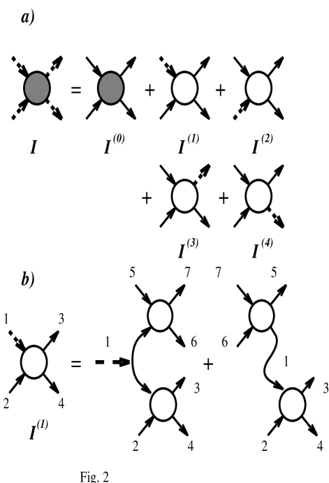
where the functions $\{\delta(\varepsilon_{p_{1}})\}_{\rm corr}$ and $\{f(\varepsilon_{p_{1}})\,\delta(\varepsilon_{p_{1}})\}_{\rm corr}$ are defined in complete analogy to eqs. (38) and (39). The explicit expression for $I^{(2)}$ follows from $I^{(1)}$ by interchanging $\mathchoice{{\hbox{\boldmath$\displaystyle p$}}}{{\hbox{\boldmath$\textstyle p$}}}{{\hbox{\boldmath$\scriptstyle p$}}}{{\hbox{\boldmath$\scriptscriptstyle p$}}}_{1}\leftrightarrow\mathchoice{{\hbox{\boldmath$\displaystyle p$}}}{{\hbox{\boldmath$\textstyle p$}}}{{\hbox{\boldmath$\scriptstyle p$}}}{{\hbox{\boldmath$\scriptscriptstyle p$}}}_{2}$, while those for $I^{(3)}$ and $I^{(4)}$ from simultaneous interchanges $\mathchoice{{\hbox{\boldmath$\displaystyle p$}}}{{\hbox{\boldmath$\textstyle p$}}}{{\hbox{\boldmath$\scriptstyle p$}}}{{\hbox{\boldmath$\scriptscriptstyle p$}}}_{4}\leftrightarrow\mathchoice{{\hbox{\boldmath$\displaystyle p$}}}{{\hbox{\boldmath$\textstyle p$}}}{{\hbox{\boldmath$\scriptstyle p$}}}{{\hbox{\boldmath$\scriptscriptstyle p$}}}_{2},\,\mathchoice{{\hbox{\boldmath$\displaystyle p$}}}{{\hbox{\boldmath$\textstyle p$}}}{{\hbox{\boldmath$\scriptstyle p$}}}{{\hbox{\boldmath$\scriptscriptstyle p$}}}_{3}\leftrightarrow\mathchoice{{\hbox{\boldmath$\displaystyle p$}}}{{\hbox{\boldmath$\textstyle p$}}}{{\hbox{\boldmath$\scriptstyle p$}}}{{\hbox{\boldmath$\scriptscriptstyle p$}}}_{1}$ and $\mathchoice{{\hbox{\boldmath$\displaystyle p$}}}{{\hbox{\boldmath$\textstyle p$}}}{{\hbox{\boldmath$\scriptstyle p$}}}{{\hbox{\boldmath$\scriptscriptstyle p$}}}_{4}\leftrightarrow\mathchoice{{\hbox{\boldmath$\displaystyle p$}}}{{\hbox{\boldmath$\textstyle p$}}}{{\hbox{\boldmath$\scriptstyle p$}}}{{\hbox{\boldmath$\scriptscriptstyle p$}}}_{1},\,\mathchoice{{\hbox{\boldmath$\displaystyle p$}}}{{\hbox{\boldmath$\textstyle p$}}}{{\hbox{\boldmath$\scriptstyle p$}}}{{\hbox{\boldmath$\scriptscriptstyle p$}}}_{3}\leftrightarrow\mathchoice{{\hbox{\boldmath$\displaystyle p$}}}{{\hbox{\boldmath$\textstyle p$}}}{{\hbox{\boldmath$\scriptstyle p$}}}{{\hbox{\boldmath$\scriptscriptstyle p$}}}_{2}$, respectively. Consistent with keeping only the first order terms in $\gamma$, the scattering amplitudes in the integrals $I^{(i)}$, $i=1,2,3,4$, are those including only the quasiparticle contributions. The first terms in the bracket in eq. (117) describes scattering of excitations, when one of these is in an initial or final correlated state. This term describes a real process with energy conservation in the scattering event and irreversible deformation of the wave functions of the scattering particles. The second term corresponds to the virtual scattering of quasiparticles with explicit nonconservation of energy and reversible deformation of the wave functions; the third term is of the coherent nature discussed above (see Fig. 2 a).

Had we preferred the decomposition in the pole and off-pole terms, then the zeroth order term would have acquired an additional factor which is a product of the wave-function renormalizations of all four quasiparticles. For the next-to-leading order virial correction one finds

$$\tilde{I}^{(1)}(\mathchoice{{\hbox{\boldmath$\displaystyle p$}}}{{\hbox{\boldmath$\textstyle p$}}}{{\hbox{\boldmath$\scriptstyle p$}}}{{\hbox{\boldmath$\scriptscriptstyle p$}}}_{1}) = \sum_{\bf p_{2}p_{3}p_{4}}\langle\mathchoice{{\hbox{\boldmath$\displaystyle p$}}}{{\hbox{\boldmath$\textstyle p$}}}{{\hbox{\boldmath$\scriptstyle p$}}}{{\hbox{\boldmath$\scriptscriptstyle p$}}}_{1},\mathchoice{{\hbox{\boldmath$\displaystyle p$}}}{{\hbox{\boldmath$\textstyle p$}}}{{\hbox{\boldmath$\scriptstyle p$}}}{{\hbox{\boldmath$\scriptscriptstyle p$}}}_{2}|W|\mathchoice{{\hbox{\boldmath$\displaystyle p$}}}{{\hbox{\boldmath$\textstyle p$}}}{{\hbox{\boldmath$\scriptstyle p$}}}{{\hbox{\boldmath$\scriptscriptstyle p$}}}_{3},\mathchoice{{\hbox{\boldmath$\displaystyle p$}}}{{\hbox{\boldmath$\textstyle p$}}}{{\hbox{\boldmath$\scriptstyle p$}}}{{\hbox{\boldmath$\scriptscriptstyle p$}}}_{4}\rangle\frac{{\cal P^{\prime}}}{\varepsilon_{p_{1}}+\varepsilon_{p_{2}}-\varepsilon_{p_{3}}-\varepsilon_{p_{4}}}\gamma(\varepsilon_{p_{3}}+\varepsilon_{p_{4}}-\varepsilon_{p_{2}})$$ (120)

$$\times \Big{\{}f(\varepsilon_{p_{3}}+\varepsilon_{p_{4}}-\varepsilon_{p_{2}})\,f(\mathchoice{{\hbox{\boldmath$\displaystyle p$}}}{{\hbox{\boldmath$\textstyle p$}}}{{\hbox{\boldmath$\scriptstyle p$}}}{{\hbox{\boldmath$\scriptscriptstyle p$}}}_{2})$$ (121)

$$\times \left[1-f(\mathchoice{{\hbox{\boldmath$\displaystyle p$}}}{{\hbox{\boldmath$\textstyle p$}}}{{\hbox{\boldmath$\scriptstyle p$}}}{{\hbox{\boldmath$\scriptscriptstyle p$}}}_{3})\right]\left[1-f(\mathchoice{{\hbox{\boldmath$\displaystyle p$}}}{{\hbox{\boldmath$\textstyle p$}}}{{\hbox{\boldmath$\scriptstyle p$}}}{{\hbox{\boldmath$\scriptscriptstyle p$}}}_{4})\right]-\left[1-f(\varepsilon_{p_{3}}+\varepsilon_{p_{4}}-\varepsilon_{p_{2}})\right]$$ (122)

$$\times \left[1-f(\mathchoice{{\hbox{\boldmath$\displaystyle p$}}}{{\hbox{\boldmath$\textstyle p$}}}{{\hbox{\boldmath$\scriptstyle p$}}}{{\hbox{\boldmath$\scriptscriptstyle p$}}}_{2})\right]f(\mathchoice{{\hbox{\boldmath$\displaystyle p$}}}{{\hbox{\boldmath$\textstyle p$}}}{{\hbox{\boldmath$\scriptstyle p$}}}{{\hbox{\boldmath$\scriptscriptstyle p$}}}_{3})\,f(\mathchoice{{\hbox{\boldmath$\displaystyle p$}}}{{\hbox{\boldmath$\textstyle p$}}}{{\hbox{\boldmath$\scriptstyle p$}}}{{\hbox{\boldmath$\scriptscriptstyle p$}}}_{4})\Big{\}}.$$ (123)

The fact that this collision integral corresponds to an effective three-body process can be visualized by inserting in the latter equation the explicit expression for the spectral width (in the quasiparticle approximation)

FIG. 2.: a) The virial decomposition of the collision integral in the two body case; the open circles denote the $T$ matrix in the quasiparticle approximation, while the filled ones include also the off-shell contributions. b) The modification of next-to-leading order correction to the gain part of the collision integral after substituting the explicit expression for the width; all the final state particles are now on the mass-shell.

$$\gamma(\mathchoice{{\hbox{\boldmath$\displaystyle p$}}}{{\hbox{\boldmath$\textstyle p$}}}{{\hbox{\boldmath$\scriptstyle p$}}}{{\hbox{\boldmath$\scriptscriptstyle p$}}}_{1}) = -\sum_{{\bf p_{2}p_{3}p_{4}}}\langle\mathchoice{{\hbox{\boldmath$\displaystyle p$}}}{{\hbox{\boldmath$\textstyle p$}}}{{\hbox{\boldmath$\scriptstyle p$}}}{{\hbox{\boldmath$\scriptscriptstyle p$}}}_{1},\mathchoice{{\hbox{\boldmath$\displaystyle p$}}}{{\hbox{\boldmath$\textstyle p$}}}{{\hbox{\boldmath$\scriptstyle p$}}}{{\hbox{\boldmath$\scriptscriptstyle p$}}}_{2}|W|\mathchoice{{\hbox{\boldmath$\displaystyle p$}}}{{\hbox{\boldmath$\textstyle p$}}}{{\hbox{\boldmath$\scriptstyle p$}}}{{\hbox{\boldmath$\scriptscriptstyle p$}}}_{3},\mathchoice{{\hbox{\boldmath$\displaystyle p$}}}{{\hbox{\boldmath$\textstyle p$}}}{{\hbox{\boldmath$\scriptstyle p$}}}{{\hbox{\boldmath$\scriptscriptstyle p$}}}_{4}\rangle(2\pi)\delta(\varepsilon_{p_{1}}+\varepsilon_{p_{2}}-\varepsilon_{p_{3}}-\varepsilon_{p_{4}})$$ (124)

$$\times \Bigl{\{}f(\mathchoice{{\hbox{\boldmath$\displaystyle p$}}}{{\hbox{\boldmath$\textstyle p$}}}{{\hbox{\boldmath$\scriptstyle p$}}}{{\hbox{\boldmath$\scriptscriptstyle p$}}}_{2})\,[1-f(\mathchoice{{\hbox{\boldmath$\displaystyle p$}}}{{\hbox{\boldmath$\textstyle p$}}}{{\hbox{\boldmath$\scriptstyle p$}}}{{\hbox{\boldmath$\scriptscriptstyle p$}}}_{3})]\,[1-f(\mathchoice{{\hbox{\boldmath$\displaystyle p$}}}{{\hbox{\boldmath$\textstyle p$}}}{{\hbox{\boldmath$\scriptstyle p$}}}{{\hbox{\boldmath$\scriptscriptstyle p$}}}_{4})]+[1-f(\mathchoice{{\hbox{\boldmath$\displaystyle p$}}}{{\hbox{\boldmath$\textstyle p$}}}{{\hbox{\boldmath$\scriptstyle p$}}}{{\hbox{\boldmath$\scriptscriptstyle p$}}}_{2})]\,f(\mathchoice{{\hbox{\boldmath$\displaystyle p$}}}{{\hbox{\boldmath$\textstyle p$}}}{{\hbox{\boldmath$\scriptstyle p$}}}{{\hbox{\boldmath$\scriptscriptstyle p$}}}_{3})\,f(\mathchoice{{\hbox{\boldmath$\displaystyle p$}}}{{\hbox{\boldmath$\textstyle p$}}}{{\hbox{\boldmath$\scriptstyle p$}}}{{\hbox{\boldmath$\scriptscriptstyle p$}}}_{4})\Bigr{\}},$$ (125)

which gives

$$I^{(1)}(\mathchoice{{\hbox{\boldmath$\displaystyle p$}}}{{\hbox{\boldmath$\textstyle p$}}}{{\hbox{\boldmath$\scriptstyle p$}}}{{\hbox{\boldmath$\scriptscriptstyle p$}}}_{1}) = \sum_{{\bf p}_{2}{\bf p}_{3}{\bf p}_{4}}\sum_{{\bf p}_{5}\,{\bf p}_{6}\,{\bf p}_{7}}\langle\mathchoice{{\hbox{\boldmath$\displaystyle p$}}}{{\hbox{\boldmath$\textstyle p$}}}{{\hbox{\boldmath$\scriptstyle p$}}}{{\hbox{\boldmath$\scriptscriptstyle p$}}}_{1},\mathchoice{{\hbox{\boldmath$\displaystyle p$}}}{{\hbox{\boldmath$\textstyle p$}}}{{\hbox{\boldmath$\scriptstyle p$}}}{{\hbox{\boldmath$\scriptscriptstyle p$}}}_{2}|W|\mathchoice{{\hbox{\boldmath$\displaystyle p$}}}{{\hbox{\boldmath$\textstyle p$}}}{{\hbox{\boldmath$\scriptstyle p$}}}{{\hbox{\boldmath$\scriptscriptstyle p$}}}_{3},\mathchoice{{\hbox{\boldmath$\displaystyle p$}}}{{\hbox{\boldmath$\textstyle p$}}}{{\hbox{\boldmath$\scriptstyle p$}}}{{\hbox{\boldmath$\scriptscriptstyle p$}}}_{4}\rangle\frac{{\cal P^{\prime}}}{\varepsilon_{p_{1}}+\varepsilon_{p_{2}}-\varepsilon_{p_{3}}-\varepsilon_{p_{4}}}$$ (126)

$$\times \Big{|}\Big{\langle}{(\mathchoice{{\hbox{\boldmath$\displaystyle p$}}}{{\hbox{\boldmath$\textstyle p$}}}{{\hbox{\boldmath$\scriptstyle p$}}}{{\hbox{\boldmath$\scriptscriptstyle p$}}}_{1}-\mathchoice{{\hbox{\boldmath$\displaystyle p$}}}{{\hbox{\boldmath$\textstyle p$}}}{{\hbox{\boldmath$\scriptstyle p$}}}{{\hbox{\boldmath$\scriptscriptstyle p$}}}_{5})/}{2}\Big{|}T^{R}(\mathchoice{{\hbox{\boldmath$\displaystyle p$}}}{{\hbox{\boldmath$\textstyle p$}}}{{\hbox{\boldmath$\scriptstyle p$}}}{{\hbox{\boldmath$\scriptscriptstyle p$}}}_{1}+\mathchoice{{\hbox{\boldmath$\displaystyle p$}}}{{\hbox{\boldmath$\textstyle p$}}}{{\hbox{\boldmath$\scriptstyle p$}}}{{\hbox{\boldmath$\scriptscriptstyle p$}}}_{5},\varepsilon_{p_{3}}+\varepsilon_{p_{4}}+\varepsilon_{p_{5}}-\varepsilon_{p_{2}},x)\Big{|}{(\mathchoice{{\hbox{\boldmath$\displaystyle p$}}}{{\hbox{\boldmath$\textstyle p$}}}{{\hbox{\boldmath$\scriptstyle p$}}}{{\hbox{\boldmath$\scriptscriptstyle p$}}}_{6}-\mathchoice{{\hbox{\boldmath$\displaystyle p$}}}{{\hbox{\boldmath$\textstyle p$}}}{{\hbox{\boldmath$\scriptstyle p$}}}{{\hbox{\boldmath$\scriptscriptstyle p$}}}_{7})/}{2}\Big{\rangle}\Big{|}^{2}$$ (127)

$$\times (2\pi)^{4}\,\delta(\mathchoice{{\hbox{\boldmath$\displaystyle p$}}}{{\hbox{\boldmath$\textstyle p$}}}{{\hbox{\boldmath$\scriptstyle p$}}}{{\hbox{\boldmath$\scriptscriptstyle p$}}}_{3}+\mathchoice{{\hbox{\boldmath$\displaystyle p$}}}{{\hbox{\boldmath$\textstyle p$}}}{{\hbox{\boldmath$\scriptstyle p$}}}{{\hbox{\boldmath$\scriptscriptstyle p$}}}_{4}+\mathchoice{{\hbox{\boldmath$\displaystyle p$}}}{{\hbox{\boldmath$\textstyle p$}}}{{\hbox{\boldmath$\scriptstyle p$}}}{{\hbox{\boldmath$\scriptscriptstyle p$}}}_{5}-\mathchoice{{\hbox{\boldmath$\displaystyle p$}}}{{\hbox{\boldmath$\textstyle p$}}}{{\hbox{\boldmath$\scriptstyle p$}}}{{\hbox{\boldmath$\scriptscriptstyle p$}}}_{2}-\mathchoice{{\hbox{\boldmath$\displaystyle p$}}}{{\hbox{\boldmath$\textstyle p$}}}{{\hbox{\boldmath$\scriptstyle p$}}}{{\hbox{\boldmath$\scriptscriptstyle p$}}}_{6}-\mathchoice{{\hbox{\boldmath$\displaystyle p$}}}{{\hbox{\boldmath$\textstyle p$}}}{{\hbox{\boldmath$\scriptstyle p$}}}{{\hbox{\boldmath$\scriptscriptstyle p$}}}_{7})~{}\delta(\varepsilon_{p_{3}}+\varepsilon_{p_{4}}+\varepsilon_{p_{5}}-\varepsilon_{p_{2}}-\varepsilon_{p_{6}}-\varepsilon_{p_{7}})$$ (128)

$$\times \Bigl{\{}f(\varepsilon_{p_{3}}+\varepsilon_{p_{4}}-\varepsilon_{p_{2}})\,f(\mathchoice{{\hbox{\boldmath$\displaystyle p$}}}{{\hbox{\boldmath$\textstyle p$}}}{{\hbox{\boldmath$\scriptstyle p$}}}{{\hbox{\boldmath$\scriptscriptstyle p$}}}_{2})\left[1-f(\mathchoice{{\hbox{\boldmath$\displaystyle p$}}}{{\hbox{\boldmath$\textstyle p$}}}{{\hbox{\boldmath$\scriptstyle p$}}}{{\hbox{\boldmath$\scriptscriptstyle p$}}}_{3})\right]\left[1-f(\mathchoice{{\hbox{\boldmath$\displaystyle p$}}}{{\hbox{\boldmath$\textstyle p$}}}{{\hbox{\boldmath$\scriptstyle p$}}}{{\hbox{\boldmath$\scriptscriptstyle p$}}}_{4})\right]$$ (129)

$$- \left[1-f(\varepsilon_{p_{3}}+\varepsilon_{p_{4}}-\varepsilon_{p_{2}})\right]\left[1-f(\mathchoice{{\hbox{\boldmath$\displaystyle p$}}}{{\hbox{\boldmath$\textstyle p$}}}{{\hbox{\boldmath$\scriptstyle p$}}}{{\hbox{\boldmath$\scriptscriptstyle p$}}}_{2})\right]f(\mathchoice{{\hbox{\boldmath$\displaystyle p$}}}{{\hbox{\boldmath$\textstyle p$}}}{{\hbox{\boldmath$\scriptstyle p$}}}{{\hbox{\boldmath$\scriptscriptstyle p$}}}_{3})\,f(\mathchoice{{\hbox{\boldmath$\displaystyle p$}}}{{\hbox{\boldmath$\textstyle p$}}}{{\hbox{\boldmath$\scriptstyle p$}}}{{\hbox{\boldmath$\scriptscriptstyle p$}}}_{4})\Bigr{\}}$$ (130)

$$\times \Bigl{\{}f(\mathchoice{{\hbox{\boldmath$\displaystyle p$}}}{{\hbox{\boldmath$\textstyle p$}}}{{\hbox{\boldmath$\scriptstyle p$}}}{{\hbox{\boldmath$\scriptscriptstyle p$}}}_{5})\left[1-f(\mathchoice{{\hbox{\boldmath$\displaystyle p$}}}{{\hbox{\boldmath$\textstyle p$}}}{{\hbox{\boldmath$\scriptstyle p$}}}{{\hbox{\boldmath$\scriptscriptstyle p$}}}_{6})\right]\left[1-f(\mathchoice{{\hbox{\boldmath$\displaystyle p$}}}{{\hbox{\boldmath$\textstyle p$}}}{{\hbox{\boldmath$\scriptstyle p$}}}{{\hbox{\boldmath$\scriptscriptstyle p$}}}_{7})\right]+\left[1-f(\mathchoice{{\hbox{\boldmath$\displaystyle p$}}}{{\hbox{\boldmath$\textstyle p$}}}{{\hbox{\boldmath$\scriptstyle p$}}}{{\hbox{\boldmath$\scriptscriptstyle p$}}}_{5})\right]f(\mathchoice{{\hbox{\boldmath$\displaystyle p$}}}{{\hbox{\boldmath$\textstyle p$}}}{{\hbox{\boldmath$\scriptstyle p$}}}{{\hbox{\boldmath$\scriptscriptstyle p$}}}_{6})\,f(\mathchoice{{\hbox{\boldmath$\displaystyle p$}}}{{\hbox{\boldmath$\textstyle p$}}}{{\hbox{\boldmath$\scriptstyle p$}}}{{\hbox{\boldmath$\scriptscriptstyle p$}}}_{7})\Bigr{\}}.$$ (131)

This result is essentially self-explanatory; the underlying process is illustrated in Fig. 2 b.

Let us turn to the collision term in the kinetic equation (53). The first term in the virial expansion is beyond the quasiparticle approximation, and e.g. for the collision term $I_{t}$ has the form

$$I_{t}^{(0)}(\mathchoice{{\hbox{\boldmath$\displaystyle p$}}}{{\hbox{\boldmath$\textstyle p$}}}{{\hbox{\boldmath$\scriptstyle p$}}}{{\hbox{\boldmath$\scriptscriptstyle p$}}}) = \sum_{{\bf p}_{2}{\bf p}_{3}{\bf p}_{4}}\frac{{\cal P^{\prime}}}{\varepsilon+\varepsilon_{p_{2}}-\varepsilon_{p_{3}}-\varepsilon_{p_{4}}}\langle\mathchoice{{\hbox{\boldmath$\displaystyle p$}}}{{\hbox{\boldmath$\textstyle p$}}}{{\hbox{\boldmath$\scriptstyle p$}}}{{\hbox{\boldmath$\scriptscriptstyle p$}}},\mathchoice{{\hbox{\boldmath$\displaystyle p$}}}{{\hbox{\boldmath$\textstyle p$}}}{{\hbox{\boldmath$\scriptstyle p$}}}{{\hbox{\boldmath$\scriptscriptstyle p$}}}_{2}|W|\mathchoice{{\hbox{\boldmath$\displaystyle p$}}}{{\hbox{\boldmath$\textstyle p$}}}{{\hbox{\boldmath$\scriptstyle p$}}}{{\hbox{\boldmath$\scriptscriptstyle p$}}}_{3},\mathchoice{{\hbox{\boldmath$\displaystyle p$}}}{{\hbox{\boldmath$\textstyle p$}}}{{\hbox{\boldmath$\scriptstyle p$}}}{{\hbox{\boldmath$\scriptscriptstyle p$}}}_{4}\rangle$$ (132)

$$\times \Bigl{\{}f(\mathchoice{{\hbox{\boldmath$\displaystyle p$}}}{{\hbox{\boldmath$\textstyle p$}}}{{\hbox{\boldmath$\scriptstyle p$}}}{{\hbox{\boldmath$\scriptscriptstyle p$}}})\,f(\mathchoice{{\hbox{\boldmath$\displaystyle p$}}}{{\hbox{\boldmath$\textstyle p$}}}{{\hbox{\boldmath$\scriptstyle p$}}}{{\hbox{\boldmath$\scriptscriptstyle p$}}}_{2})[1-f(\mathchoice{{\hbox{\boldmath$\displaystyle p$}}}{{\hbox{\boldmath$\textstyle p$}}}{{\hbox{\boldmath$\scriptstyle p$}}}{{\hbox{\boldmath$\scriptscriptstyle p$}}}_{3})][1-f(\mathchoice{{\hbox{\boldmath$\displaystyle p$}}}{{\hbox{\boldmath$\textstyle p$}}}{{\hbox{\boldmath$\scriptstyle p$}}}{{\hbox{\boldmath$\scriptscriptstyle p$}}}_{4})]+[1-f(\mathchoice{{\hbox{\boldmath$\displaystyle p$}}}{{\hbox{\boldmath$\textstyle p$}}}{{\hbox{\boldmath$\scriptstyle p$}}}{{\hbox{\boldmath$\scriptscriptstyle p$}}})][1-f(\mathchoice{{\hbox{\boldmath$\displaystyle p$}}}{{\hbox{\boldmath$\textstyle p$}}}{{\hbox{\boldmath$\scriptstyle p$}}}{{\hbox{\boldmath$\scriptscriptstyle p$}}}_{2})]f(\mathchoice{{\hbox{\boldmath$\displaystyle p$}}}{{\hbox{\boldmath$\textstyle p$}}}{{\hbox{\boldmath$\scriptstyle p$}}}{{\hbox{\boldmath$\scriptscriptstyle p$}}}_{3})\,f(\mathchoice{{\hbox{\boldmath$\displaystyle p$}}}{{\hbox{\boldmath$\textstyle p$}}}{{\hbox{\boldmath$\scriptstyle p$}}}{{\hbox{\boldmath$\scriptscriptstyle p$}}}_{4})\Bigr{\}}.$$ (133)

Compared with the first term of the virial expansion of the regular collision integral $I(\mathchoice{{\hbox{\boldmath$\displaystyle p$}}}{{\hbox{\boldmath$\textstyle p$}}}{{\hbox{\boldmath$\scriptstyle p$}}}{{\hbox{\boldmath$\scriptscriptstyle p$}}},x)$ this term differs by the off-shell energy denominator; in contrast to the virial correction terms here all four particles are in the final on-shell states, however their energies are not matched by the energy conservation condition. The latter expression defines the correlated part of the distribution function as a functional of the on-shell QP distribution function via integral form of the kinetic equation (53).

V Virial Corrections in Equilibrium

When integrated over momentum the kinetic equation provides number density conservation; in the equilibrium limit the conserved density is the sum of quasiparticle density and the density of correlated excitations

$$n_{\rm tot}(\mathchoice{{\hbox{\boldmath$\displaystyle r$}}}{{\hbox{\boldmath$\textstyle r$}}}{{\hbox{\boldmath$\scriptstyle r$}}}{{\hbox{\boldmath$\scriptscriptstyle r$}}})=n_{\rm free}(\mathchoice{{\hbox{\boldmath$\displaystyle r$}}}{{\hbox{\boldmath$\textstyle r$}}}{{\hbox{\boldmath$\scriptstyle r$}}}{{\hbox{\boldmath$\scriptscriptstyle r$}}})+n_{\rm corr}(\mathchoice{{\hbox{\boldmath$\displaystyle r$}}}{{\hbox{\boldmath$\textstyle r$}}}{{\hbox{\boldmath$\scriptstyle r$}}}{{\hbox{\boldmath$\scriptscriptstyle r$}}})=\int\!\frac{d^{3}p}{(2\pi)^{3}}\left[f(\varepsilon_{p},\mathchoice{{\hbox{\boldmath$\displaystyle r$}}}{{\hbox{\boldmath$\textstyle r$}}}{{\hbox{\boldmath$\scriptstyle r$}}}{{\hbox{\boldmath$\scriptscriptstyle r$}}})+\{f(\varepsilon_{p},\mathchoice{{\hbox{\boldmath$\displaystyle r$}}}{{\hbox{\boldmath$\textstyle r$}}}{{\hbox{\boldmath$\scriptstyle r$}}}{{\hbox{\boldmath$\scriptscriptstyle r$}}})\}_{\rm corr}\right].$$ (134)

Consistent with our approximations, the equation of state contains virial corrections up to the third order. Before giving the expression for the third quantum virial coefficient let us briefly recapitulate the second virial coefficient (see also  [20]).

A The Second Virial Coefficient

The starting expression is that for the width at the two-body $T$-matrix level

$$\gamma(p_{1}) = -2i\sum_{p_{2}}\{\langle(\mathchoice{{\hbox{\boldmath$\displaystyle p$}}}{{\hbox{\boldmath$\textstyle p$}}}{{\hbox{\boldmath$\scriptstyle p$}}}{{\hbox{\boldmath$\scriptscriptstyle p$}}}_{1}-\mathchoice{{\hbox{\boldmath$\displaystyle p$}}}{{\hbox{\boldmath$\textstyle p$}}}{{\hbox{\boldmath$\scriptstyle p$}}}{{\hbox{\boldmath$\scriptscriptstyle p$}}}_{2})/2|{\rm Im}T^{R}(p_{1}+p_{2})|(\mathchoice{{\hbox{\boldmath$\displaystyle p$}}}{{\hbox{\boldmath$\textstyle p$}}}{{\hbox{\boldmath$\scriptstyle p$}}}{{\hbox{\boldmath$\scriptscriptstyle p$}}}_{1}-\mathchoice{{\hbox{\boldmath$\displaystyle p$}}}{{\hbox{\boldmath$\textstyle p$}}}{{\hbox{\boldmath$\scriptstyle p$}}}{{\hbox{\boldmath$\scriptscriptstyle p$}}}_{2})/2\rangle\,G^{<}(p_{2})$$ (135)

$$- \langle{(\mathchoice{{\hbox{\boldmath$\displaystyle p$}}}{{\hbox{\boldmath$\textstyle p$}}}{{\hbox{\boldmath$\scriptstyle p$}}}{{\hbox{\boldmath$\scriptscriptstyle p$}}}_{1}-\mathchoice{{\hbox{\boldmath$\displaystyle p$}}}{{\hbox{\boldmath$\textstyle p$}}}{{\hbox{\boldmath$\scriptstyle p$}}}{{\hbox{\boldmath$\scriptscriptstyle p$}}}_{2})/}{2}|T^{<}(p_{1}+p_{2})|(\mathchoice{{\hbox{\boldmath$\displaystyle p$}}}{{\hbox{\boldmath$\textstyle p$}}}{{\hbox{\boldmath$\scriptstyle p$}}}{{\hbox{\boldmath$\scriptscriptstyle p$}}}_{1}-\mathchoice{{\hbox{\boldmath$\displaystyle p$}}}{{\hbox{\boldmath$\textstyle p$}}}{{\hbox{\boldmath$\scriptstyle p$}}}{{\hbox{\boldmath$\scriptscriptstyle p$}}}_{2})/{2}\rangle\,{\rm Im}G^{R}(p_{2})\}.$$ (136)

First we simplify this expression by eliminating the $T^{<}$ function using the optical theorem (103) in equilibrium. The latter can be transformed, using the operator relation $2\,{\rm Im}T^{R}=i(T^{<}-T^{>})$, to the following form:

$$\langle\mathchoice{{\hbox{\boldmath$\displaystyle p$}}}{{\hbox{\boldmath$\textstyle p$}}}{{\hbox{\boldmath$\scriptstyle p$}}}{{\hbox{\boldmath$\scriptscriptstyle p$}}}_{1}|{\rm Im}T^{R}(P)|\mathchoice{{\hbox{\boldmath$\displaystyle p$}}}{{\hbox{\boldmath$\textstyle p$}}}{{\hbox{\boldmath$\scriptstyle p$}}}{{\hbox{\boldmath$\scriptscriptstyle p$}}}_{2}\rangle = -\frac{1}{2}\sum_{p_{3}p_{4}}a(\omega_{3})\,a(\omega_{4})\langle\mathchoice{{\hbox{\boldmath$\displaystyle p$}}}{{\hbox{\boldmath$\textstyle p$}}}{{\hbox{\boldmath$\scriptstyle p$}}}{{\hbox{\boldmath$\scriptscriptstyle p$}}}_{1}|T^{R}(P)|{(\mathchoice{{\hbox{\boldmath$\displaystyle p$}}}{{\hbox{\boldmath$\textstyle p$}}}{{\hbox{\boldmath$\scriptstyle p$}}}{{\hbox{\boldmath$\scriptscriptstyle p$}}}_{3}-\mathchoice{{\hbox{\boldmath$\displaystyle p$}}}{{\hbox{\boldmath$\textstyle p$}}}{{\hbox{\boldmath$\scriptstyle p$}}}{{\hbox{\boldmath$\scriptscriptstyle p$}}}_{4})/}{2}\rangle\,\left[1-f(\omega_{3})-f(\omega_{4})\right]$$ (137)

$$\times \langle{(\mathchoice{{\hbox{\boldmath$\displaystyle p$}}}{{\hbox{\boldmath$\textstyle p$}}}{{\hbox{\boldmath$\scriptstyle p$}}}{{\hbox{\boldmath$\scriptscriptstyle p$}}}_{3}-\mathchoice{{\hbox{\boldmath$\displaystyle p$}}}{{\hbox{\boldmath$\textstyle p$}}}{{\hbox{\boldmath$\scriptstyle p$}}}{{\hbox{\boldmath$\scriptscriptstyle p$}}}_{4})/}{2}|T^{A}(P)|\mathchoice{{\hbox{\boldmath$\displaystyle p$}}}{{\hbox{\boldmath$\textstyle p$}}}{{\hbox{\boldmath$\scriptstyle p$}}}{{\hbox{\boldmath$\scriptscriptstyle p$}}}_{2}\rangle\,(2\pi)^{4}\delta(P-p_{3}-p_{4}),$$ (138)

where $f(\omega)=\left[{\rm exp}\left(\beta(\omega-\mu)\right)+1\right]^{-1}$ is the Fermi distribution function, $\mu$ being the chemical potential, and $\beta$ the inverse temperature. Introducing the distribution functions in the eq. (103), noting that in equilibrium

$$f(\omega_{1})f(\omega_{2})=g(\omega_{1}+\omega_{2})\,[1-f(\omega_{1})-f(\omega_{2})],$$

where $g(\omega)=\left[{\rm exp}\left(\beta(\omega-\mu)\right)-1\right]^{-1}$ is the Bose distribution function, and comparing eqs. (103) and (137) one finds that

$$\langle\mathchoice{{\hbox{\boldmath$\displaystyle p$}}}{{\hbox{\boldmath$\textstyle p$}}}{{\hbox{\boldmath$\scriptstyle p$}}}{{\hbox{\boldmath$\scriptscriptstyle p$}}}_{1}|T^{<}(P)|\mathchoice{{\hbox{\boldmath$\displaystyle p$}}}{{\hbox{\boldmath$\textstyle p$}}}{{\hbox{\boldmath$\scriptstyle p$}}}{{\hbox{\boldmath$\scriptscriptstyle p$}}}_{2}\rangle=-2i\,g(\omega_{1}+\omega_{2})\,\langle\mathchoice{{\hbox{\boldmath$\displaystyle p$}}}{{\hbox{\boldmath$\textstyle p$}}}{{\hbox{\boldmath$\scriptstyle p$}}}{{\hbox{\boldmath$\scriptscriptstyle p$}}}_{1}|{\rm Im}T^{R}(P)|\mathchoice{{\hbox{\boldmath$\displaystyle p$}}}{{\hbox{\boldmath$\textstyle p$}}}{{\hbox{\boldmath$\scriptstyle p$}}}{{\hbox{\boldmath$\scriptscriptstyle p$}}}_{2}\rangle.$$ (139)

The expression for the width $\gamma(p)$ simplifies to

$$\gamma(p_{1})=2\sum_{p_{2}}a(\omega_{2})\,\left[g(\omega_{1}+\omega_{2})+f(\omega_{2})\right]\langle{(\mathchoice{{\hbox{\boldmath$\displaystyle p$}}}{{\hbox{\boldmath$\textstyle p$}}}{{\hbox{\boldmath$\scriptstyle p$}}}{{\hbox{\boldmath$\scriptscriptstyle p$}}}_{1}-\mathchoice{{\hbox{\boldmath$\displaystyle p$}}}{{\hbox{\boldmath$\textstyle p$}}}{{\hbox{\boldmath$\scriptstyle p$}}}{{\hbox{\boldmath$\scriptscriptstyle p$}}}_{2})/}{2}|{\rm Im}T^{R}(p_{1}+p_{2})|{(\mathchoice{{\hbox{\boldmath$\displaystyle p$}}}{{\hbox{\boldmath$\textstyle p$}}}{{\hbox{\boldmath$\scriptstyle p$}}}{{\hbox{\boldmath$\scriptscriptstyle p$}}}_{1}-\mathchoice{{\hbox{\boldmath$\displaystyle p$}}}{{\hbox{\boldmath$\textstyle p$}}}{{\hbox{\boldmath$\scriptstyle p$}}}{{\hbox{\boldmath$\scriptscriptstyle p$}}}_{2})/}{2}\rangle.$$ (140)

Substituting the expression for $\gamma(p)$, eq. (124), in the expression for the correlated density and using the equilibrium identity

$$\left[g(E)+f(\omega_{2})\right]\left[f(E-\omega_{2})-f(\omega_{1})\right]=\left[g(E)-g(\omega_{1}+\omega_{2})\right]\left[1-f(\omega_{1})-f(\omega_{2})\right],$$ (141)

one finds the following form of the two-particle correlation function [23, 24, 25]

$$\{f^{II}(\varepsilon_{p_{1}})\}_{\rm corr}=\int\!\frac{dE}{2\pi}g(E)b(\varepsilon_{p_{1}},E),$$ (142)

where

$$b(\varepsilon_{p_{1}},E) = 2\sum_{{\bf p}_{2}}\left[1-f(\varepsilon_{p_{1}})-f(\varepsilon_{p_{2}})\right]\{\langle(\mathchoice{{\hbox{\boldmath$\displaystyle p$}}}{{\hbox{\boldmath$\textstyle p$}}}{{\hbox{\boldmath$\scriptstyle p$}}}{{\hbox{\boldmath$\scriptscriptstyle p$}}}_{1}-\mathchoice{{\hbox{\boldmath$\displaystyle p$}}}{{\hbox{\boldmath$\textstyle p$}}}{{\hbox{\boldmath$\scriptstyle p$}}}{{\hbox{\boldmath$\scriptscriptstyle p$}}}_{2})/2|{\rm Im}T^{R}(E)|(\mathchoice{{\hbox{\boldmath$\displaystyle p$}}}{{\hbox{\boldmath$\textstyle p$}}}{{\hbox{\boldmath$\scriptstyle p$}}}{{\hbox{\boldmath$\scriptscriptstyle p$}}}_{1}-\mathchoice{{\hbox{\boldmath$\displaystyle p$}}}{{\hbox{\boldmath$\textstyle p$}}}{{\hbox{\boldmath$\scriptstyle p$}}}{{\hbox{\boldmath$\scriptscriptstyle p$}}}_{2})/2\rangle\frac{d}{dE}{\rm Re}{R}^{R}(E)$$ (143)

$$+ {\rm Im}{R}^{R}(E)\,\frac{d}{dE}\langle(\mathchoice{{\hbox{\boldmath$\displaystyle p$}}}{{\hbox{\boldmath$\textstyle p$}}}{{\hbox{\boldmath$\scriptstyle p$}}}{{\hbox{\boldmath$\scriptscriptstyle p$}}}_{1}-\mathchoice{{\hbox{\boldmath$\displaystyle p$}}}{{\hbox{\boldmath$\textstyle p$}}}{{\hbox{\boldmath$\scriptstyle p$}}}{{\hbox{\boldmath$\scriptscriptstyle p$}}}_{2})/2|{\rm Im}T^{R}(E)|(\mathchoice{{\hbox{\boldmath$\displaystyle p$}}}{{\hbox{\boldmath$\textstyle p$}}}{{\hbox{\boldmath$\scriptstyle p$}}}{{\hbox{\boldmath$\scriptscriptstyle p$}}}_{1}-\mathchoice{{\hbox{\boldmath$\displaystyle p$}}}{{\hbox{\boldmath$\textstyle p$}}}{{\hbox{\boldmath$\scriptstyle p$}}}{{\hbox{\boldmath$\scriptscriptstyle p$}}}_{2})/2\rangle\}$$ (144)

is the two-particle spectral function and $R$ is the two-particle resolvent.

B The Third Virial Coefficient

To derive the third virial coefficient we first relate the ${\cal T^{<,>}}$ matrices to the imaginary part of the retarded ${\cal T}^{R}$- matrix. The optical theorem reads

$$\langle\mbox{\boldmath$k$}_{23}\mbox{\boldmath$q$}_{1}|{\rm Im}{\cal T}^{R}(K)|\mbox{\boldmath$k$}_{45}\mbox{\boldmath$q$}_{6}\rangle = \frac{i}{2}\sum_{\alpha\beta}\sum_{p_{4},p_{5},p_{6}}\langle\mbox{\boldmath$k$}_{23}\mbox{\boldmath$q$}_{1}|{\cal T}^{R\,(\alpha)}(K)|\mbox{\boldmath$k$}_{45}\mbox{\boldmath$q$}_{6}\rangle\Bigl{[}G^{<}(p_{4})G^{<}(p_{5})G^{<}(p_{6})$$ (145)

$$- G^{>}(p_{4})G^{>}(p_{5})G^{>}(p_{6})\Bigr{]}\langle\mbox{\boldmath$k$}_{45}\mbox{\boldmath$q$}_{6}|{\cal T}^{A\,(\beta)}(K)|\mbox{\boldmath$k$}_{23}\mbox{\boldmath$q$}_{1}\rangle$$ (146)

$$\times \delta^{4}\left(K-p_{4}-p_{5}-p_{6}\right).$$ (147)

where the momenta $p_{i}$ $i=1\dots 6$ are related to $k_{\alpha\beta},q_{\gamma}$ via relations (77). Using the equilibrium identity

$$f(\omega_{1})f(\omega_{2})f(\omega_{3}) = f(\omega_{1}+\omega_{2}+\omega_{3})\Bigl{[}1-f(\omega_{1})-f(\omega_{2})-f(\omega_{3})+f(\omega_{1})f(\omega_{2})$$ (148)

$$+ f(\omega_{1})f(\omega_{3})+f(\omega_{2})f(\omega_{3})\Bigr{]},$$ (149)

one finds in the QP limit:

$$\langle\mbox{\boldmath$k$}_{23}\mbox{\boldmath$q$}_{1}|{\cal T}^{<}(K)|\mbox{\boldmath$k$}_{45}\mbox{\boldmath$q$}_{6}\rangle = 2if\left(\omega_{1}+\omega_{2}+\omega_{3}\right)\langle\mbox{\boldmath$k$}_{23}\mbox{\boldmath$q$}_{1}|{\rm Im}{\cal T}^{R}(K)|\mbox{\boldmath$k$}_{45}\mbox{\boldmath$q$}_{6}\rangle,$$ (150)

$$\langle\mbox{\boldmath$k$}_{23}\mbox{\boldmath$q$}_{1}|{\cal T}^{>}(K)|\mbox{\boldmath$k$}_{45}\mbox{\boldmath$q$}_{6}\rangle = 2i\left[1-f\left(\omega_{1}+\omega_{2}+\omega_{3}\right)\right]\langle\mbox{\boldmath$k$}_{23}\mbox{\boldmath$q$}_{1}|{\rm Im}{\cal T}^{R}(K)|\mbox{\boldmath$k$}_{45}\mbox{\boldmath$q$}_{6}\rangle.$$ (151)

The three-particle correlation function takes the form

$$\{f^{III}(\varepsilon_{p_{1}})\}_{\rm corr} = -2i\int\!\frac{d\omega}{2\pi}\sum_{p_{2},p_{3}}\langle\mbox{\boldmath$k$}_{23}\mbox{\boldmath$q$}_{1}|{\rm Im}{\cal T}^{R}(K)|\mbox{\boldmath$k$}_{23}\mbox{\boldmath$q$}_{1}\rangle\left[f\left(\omega_{1}+\varepsilon_{p_{2}}+\varepsilon_{p_{3}}\right)+g(\varepsilon_{p_{2}}+\varepsilon_{p_{3}})\right]$$ (152)

$$\times \left[1-f(\varepsilon_{p_{2}})-f(\varepsilon_{p_{3}})\right]\,\left[f(\omega)-f(\varepsilon_{p_{1}})\right]\frac{{\cal P^{\prime}}}{\varepsilon_{p_{1}}-\omega}.$$ (153)

Next we use the identity, valid in equilibrium,

$$\left[f(\omega+\varepsilon_{p_{2}}+\varepsilon_{p_{3}})+g(\varepsilon_{p_{2}}+\varepsilon_{p_{3}})\right]\left[1-f(\varepsilon_{p_{2}})-f(\varepsilon_{p_{3}})\right]\left[f(\omega)-f(\varepsilon_{p_{1}})\right]$$ (154)

$$= \left[f(E)-f(\varepsilon_{p_{1}}+\varepsilon_{p_{2}}+\varepsilon_{p_{3}})\right]\Bigl{[}1-f(\varepsilon_{p_{1}})-f(\varepsilon_{p_{2}})-f(\varepsilon_{p_{3}})+f(\varepsilon_{p_{1}})f(\varepsilon_{p_{2}})$$ (155)

$$+ f(\varepsilon_{p_{1}})f(\varepsilon_{p_{3}})+f(\varepsilon_{p_{2}})f(\varepsilon_{p_{3}})\Bigr{]},$$ (156)

where $E=\omega+\varepsilon_{p_{2}}+\varepsilon_{p_{3}}$. After the substitution in eq. (152) the desired form of the correlation function is found

$$\{f^{III}(\varepsilon_{p_{1}})\}_{\rm corr}=\int\!\frac{dE}{2\pi}f(E)~{}c(\varepsilon_{p_{1}},E),$$ (157)

where the third order quantum virial coefficient is defined as

$$c(\varepsilon_{p_{1}},E) = 2\sum_{{\bf p}_{2}{\bf p}_{3}}\Bigl{[}1-f(\varepsilon_{p_{1}})-f(\varepsilon_{p_{2}})-f(\varepsilon_{p_{3}})+f(\varepsilon_{p_{1}})f(\varepsilon_{p_{2}})+f(\varepsilon_{p_{1}})f(\varepsilon_{p_{3}})+f(\varepsilon_{p_{2}})f(\varepsilon_{p_{3}})\Bigr{]}$$ (158)

$$\times \left[\langle\mbox{\boldmath$k$}_{23}\mbox{\boldmath$q$}_{1}|{\rm Im}{\cal T}^{R}(K)|\mbox{\boldmath$k$}_{23}\mbox{\boldmath$q$}_{1}\rangle\frac{d}{dE}{\rm Re}{\cal R}(E)+{\rm Im}{\cal R}(E)\frac{d}{dE}\langle\mbox{\boldmath$k$}_{23}\mbox{\boldmath$q$}_{1}|{\rm Re}{\cal T}(K)|\mbox{\boldmath$k$}_{23}\mbox{\boldmath$q$}_{1}\rangle\right]$$ (159)

and where ${\cal R}=\left[E-\varepsilon_{p_{1}}-\varepsilon_{p_{2}}-\varepsilon_{p_{3}}+i\eta\right]^{-1}$is the three-particle resolvent.

Collecting the results, the virial expansion for the density reads

$$n_{\rm tot}=\int\!\frac{d^{3}pdE}{(2\pi)^{4}}\left[a(E,\varepsilon_{p})~{}f(E)+b(E,\varepsilon_{p})~{}g(E)+c(E,\varepsilon_{p})~{}f(E)\right].$$ (160)

This expression extends the quantum virial expansion for equilibrium Fermi-systems to terms of the third order in density. We note that the last term, as in the two-body case [23, 24, 25], can be separated further into bound and scattering contributions, which can then be expressed through the in-medium three-body scattering phase-shifts.

VI Summary

In this paper, we derived coupled quantum kinetic equations for Fermi-systems in the framework of real-time Green’s function theory. The quasiclassical double-time Kadanoff-Baym equation was reduced to two single-time Boltzmann-type equations for quasiparticles and off-mass-shell excitations which are coupled via generalized scattering integrals. The part of correlations related to the off-mass-shell excitations are accounted for via an expansion of the spectral function up to the next-to-leading order terms in spectral width [21, 22], which is regarded as a small parameter. Although the treatment of the drift part is conceptually close to refs.  [21, 22], we show that a different partition of the quasiclassical functions with respect to the orders of the spectral width can be exploited with the same efficiency as the separation in pole and off-pole contributions. In particular, the latter partition has the advantage that it fulfills the spectral sum rule at each order of the decomposition and, in addition, closely parallels the equilibrium treatments based on the same approximation to the spectral function [23, 24, 25], thus providing a consistency check for the variables treated in the local equilibrium limit (e.g. scattering amplitudes).

The collision integrals contain contributions from three-body scattering. The three-particle scattering amplitudes are determined by mapping the Faddeev decomposition on the time-contour. The resulting in-medium three-body equations contain the effects of the statistical suppression of the intermediate state three-particle propagation and quasiparticle renormalization; in the vacuum limit they reduce to the well-known Faddeev equations for the three-particle problem in free space [26]. The amplitudes derived in this manner differ from those considered by Bezzerides and DuBois  [28] in that they resum the complete series in the particle-particle channel and are free of divergences associated with the non-Fredholm nature of the kernel of the three-body integral equation for the amplitudes. Our equations appear to be consistent with the time-local limit of the 2-particle–hole equations derived in the self-consistent random-phase approximation [17, 29, 30, 31].

The decomposition of the scattering integrals in the on- and off-shell parts is accomplished in much the same manner as for the scattering amplitudes. The zeroth order term is the familiar Landau collision integral in the $T$-matrix approximation [1, 14, 17]. Four further terms represent first order virial corrections to this collision integral, with one of the incoming or outgoing particles being in an off-mass-shell state. Consistent with keeping only the first order terms in the width, the transition probabilities enter the zeroth order term of the virial expansion with the full off-shell contribution, while the first order terms acquire only on-shell (zeroth order) contributions. A similar expansion holds for the kinetic equation for correlated elementary excitations. The scattering processes that contain an off-shell particle in the final state can further be expanded, putting all final states on the mass-shell: one then finds that these processes effectively correspond to successive two-body scattering events connected by an intermediate off-shell propagation.

In the equilibrium limit the equation of state has the form of a virial expansion and is truncated at the level of the three-body correlation. An explicit expression for the third quantum virial coefficient, which is expressed via the three-body scattering amplitudes and the three particle resolvent, is obtained. The latter result extends previous discussions of the quantum Beth-Uhlenbeck formula for the density including the two-body correlation [23, 24, 25] to the three-body case.

Numerical studies of three-body correlations at finite temperatures and densities in the context of excited nuclear matter using the full three-body equations either in the AGS or Faddeev formulation are underway. The in-medium nucleon-deuteron cross-section has been calculated recently [33], and the relaxation times for the nucleon-deuteron system have been estimated [34]. The Mott-dissociation of tritium in hot nuclear matter is now being studied.

REFERENCES

- [1] G. Baym and C. J. Pethick, “Landau Fermi-Liquid Theory”, Wiley, New York, 1991.
- [2] E. M. Lifshitz and L. P. Pitaevskii, “Physical Kinetics”, Pergamon, Oxford, 1981.
- [3] D. N. Zubarev, V. G. Morozov, and G. Röpke, “Statistical Mechanics of Nonequilibrium Processes”, vol. I, Akademie Verlag, Berlin, 1996.
- [4] G. F. Bertsch and Das Gupta, Phys. Rep. 160 (1988), 185.
- [5] M. Baldo, U. Lombardo, and P. Schuck, Phys. Rev. C 52 (1995), 975.
- [6] P. Danielewicz and G. F. Bertsch, Nucl. Phys. A 533 (1991), 712.
- [7] G. Röpke and H. Schulz, Nucl. Phys. A 477 (1988), 472.
- [8] J. Knoll and D. N. Voskresensky, Ann. Phys. (NY) 249 (1996), 532, and references therein.
- [9] E. G. D. Cohen, Physica A 194 (1993), 229.
- [10] R. F. Snyder, Journ. Stat. Phys. 61 (1990), 443. ibid. 63 (1991), 707.
- [11] F. Lalöe and W. J. Mullin, Journ. Stat. Phys. 59 (1990), 725.
- [12] J. A. McLennan, Journ. Stat. Phys. 28 (1982), 521.
- [13] Y. L. Klimontovich, D. Kremp, and W. D. Kraeft, “Advances in Chemical Physics”, Wiley, New York, 1987.
- [14] L. P. Kadanoff and G. Baym, “Quantum Statistical Mechanics” Benjamin, New York, 1962.
- [15] L. V. Keldysh, Sov. Phys. JETP 20 (1965), 1018.
- [16] J. W. Serene and D. Reiner, Phys. Rep. 101 (1983), 221
- [17] P. Danielewicz, Ann. Phys. (NY) 152 (1984), 239; ibid. 197 (1990), 154.
- [18] A. G. Aronov, Yu. M. Gal’perin, V. L. Gurevich and V. I. Kozub in “Nonequilibrium Superconductivity” (D. N. Langenberg and A. I. Larkin, Eds.) p. 325, North Holland, Amsterdam, 1986.
- [19] W. Botermans and R. Malfliet, Phys. Rep. 198 (1990), 115.
- [20] K. Morawetz and G. Röpke, Phys. Rev. E 51 (1995), 4246.
- [21] V. Špička and P. Lipavský, K. Morawetz, Phys. Rev. B 55 (1997), 5095.
- [22] V. Špička and P. Lipavský, Phys. Rev B 52 (1995), 14615.
- [23] R. Zimmermann and H. Stolz, Phys. Status Solidi B 131 (1985), 151; ibid. 94, (1979), 139.
- [24] D. Kremp, W. D. Kraeft, and A. J. M. D. Lambert, Physica A 127, (1984), 72.
- [25] M. Schmidt, G. Röpke and H. Schulz, Ann. Phys. (NY) 202 (1990), 57.
- [26] L. D. Faddeev, Sov. Phys. JETP 39 (1960), 139.
- [27] E. O. Alt, P. Grassberger, and W. Sandhas, Nucl. Phys. B 2, (1967), 167.
- [28] B. Bezzerides and D. F. DuBois, Phys. Rev. 186 (1968), 233.
- [29] P. Schuck, F. Villars, and P. Ring, Nucl. Phys. A 208 (1973), 302.
- [30] P. Schuck, Nucl. Phys. A 567 (1994), 78.
- [31] J. Dukelsky and P. Schuck, Nucl. Phys. A 512 (1990), 466.
- [32] P. Danielewicz and P. Schuck, Nucl. Phys. A 566 (1994), 23.
- [33] M. Beyer, G. Röpke and A. Sedrakian, Phys. Lett. B 376 (1996), 7.
- [34] M. Beyer and G. Röpke, Phys. Rev. C 56 (1997) 2636.
- [35] K. A. Brueckner, and J. L. Gammel, Phys. Rev. 109, (1958), 1023.
- [36] V. M. Galitskii, Sov. Phys. JETP 7 (1958), 104.
- [37] D. J. Thouless, Ann. Phys. (NY) 10 (1960), 553.
- [38] A. Sedrakian, Th. Alm and U. Lombardo, Phys. Rev. C 55 (1996), R582.
- [39] H. Heiselberg, C. J. Pethick and D. G. Ravenhall, Ann. Phys. (NY) 223 (1993), 37.
- [40] G. Röpke, K. Morawetz and Th. Alm, Phys. Lett. A 194 (1994), 1.
- [41] G. Röpke et al., Nucl. Phys. A 399, (1983) 587.
- [42] D. Kremp, M. Schlanges, Th Bornath, Journ. Stat. Phys. 41 (1985), 661.