MSUCL-1086 Optimized Discretization of Sources
Imaged in Heavy-Ion Reactions

Abstract

We develop the new method of optimized discretization for imaging the relative source from two particle correlation functions. In this method, the source resolution depends on the relative particle separation and is adjusted to available data and their errors. We test the method by restoring assumed pp sources and then apply the method to pp and IMF data. In reactions below 100 MeV/nucleon, significant portions of the sources extend to large distances ($r>20$ fm). The results from the imaging show the inadequacy of common Gaussian source-parametrizations. We establish a simple relation between the height of the pp correlation function and the source value at short distances, and between the height and the proton freeze-out phase-space density.

I Introduction

Imaging techniques are used in many diverse areas such as geophysics, astronomy, medical diagnostics, and police work. The goal of imaging varies widely from determining the density of the Earth’s interior to reading license plates from blurred photographs to issue speeding fines. A typical linear imaging problem involves extracting a source from measured data, where the data is represented as the convolution of a kernel with a source. An example of this is imaging the relative source function $S_{{\bf P}}({\bf r})$ from the two–particle correlation function, $C_{{\bf P}}({\bf q})$, often measured in nuclear reactions [1]:

$$C_{{\bf P}}({\bf q})-1\equiv{\cal R}_{{\bf P}}({\bf q})=\int d{\bf r}\,K({\bf q},{\bf r})\,S_{{\bf P}}({\bf r})\,.$$ (1)

Here ${\bf P}$ is the total momentum of the particle pair and the kernel $K$ is is equal to [2, 3, 4]

$$K({\bf q},{\bf r})=|\Phi_{{\bf q}}^{(-)}({\bf r})|^{2}-1\,.$$ (2)

The wavefunction $\Phi^{(-)}$ describes the propagation of the pair from a cm separation ${\bf r}$ out to the detector at infinity, where relative momentum ${\bf q}$ is reached. In the semiclassical limit, the relative source $S_{\bf P}$ for any two particles represents the probability distribution for emitting the the two particles with a separation ${\bf r}$, in their center of mass.

On the face of it, imaging appears straightforward: in the case of the two–particle correlation function, one could just discretize $C_{{\bf P}}$ and $S_{{\bf P}}$ and invert the resulting matrix equation. However, in practice this may not work as small variations in data, within statistical or systematic errors, can generate huge changes in the imaged source. This stability problem is well known in other fields and vast literature exists on its resolution [5, 6, 7, 8, 9]. In fact, many imaging problems [10, 7] that are now routinely solved would be considered ill-posed in the sense of Hadamard, who discussed stability in inversion as early as in 1923 [11]. A key element in stabilizing the inversion process was found by Tikhonov [12] who showed that inversion problems can be regularized by using known constraints satisfied by the source. Thus, in optical imaging (e.g. in astronomy) the most common method is the maximum entropy method [13, 14, 7]. The maximum entropy method works by using the most likely (i.e. uniform) image at scales below the resolution limit to stabilize the restored image at larger scales. In this method, the image is constrained to be positive. In this paper, we describe a method for imaging the relative source function from the two–particle correlation function, without explicit constraints. Our new method is similar in spirit to the maximum entropy method in that we optimize the scale of the kernel $K$ and then use the optimized scale to restore the actual source (i.e. the entire image).

In a recent paper [1], we demonstrated that it is possible to image the relative sources in heavy-ion reactions. This represented a step forward as, in the past, the integral relation between the correlation functions and the sources was only used to determine the gross features of the sources, such as representative radii. In [1] we put forward two methods of imaging sources from correlations. In the first of these methods, we used the fact that, when mutual interactions could be ignored or easily corrected such as with photons or pions, the kernel is dominated by Bose–Einstein interference. The kernel then becomes a cosine and imaging turns to inverting a Fourier cosine transform. The method allowed us to determine source values for any separation within a certain range. In the second method, we simply discretized the source at equal intervals. This method is more general and can be applied to such cases as proton-proton (pp) correlations. We did not discuss the stability of either of these methods.

The question that we now ask is whether discretizing the source at equal intervals is optimal in our second, more general, imaging method [1]. For example, in the pp case, the correlation function is dominated by the Coulomb interaction at low-relative momenta and by the strong interaction and antisymmetrization at intermediate momenta. The different momentum regions should give access to large and short distances within the source, respectively, with the resolution decreasing at the large distances, rather than being fixed. This suggests that, by varying the size of the discretization interval, we can optimize the kernel to best restore a given source. Since we do not know the source ahead of time, we must specify an “model source” in order to choose the best kernel. This kernel is then used in the actual inversion process.

We illustrate the seriousness of the stability problems by constructing a test correlation function, with errors, out of an assumed source and attempting to restore the source. Next, we demonstrate how our method stabilizes the inversion. Following this, we apply the new method to the pp data [15, 16] already analyzed in [1]. We assess whether the sources are positive definite, which would allow for their semiclassical interpretation. We compare the results to results from the transport model of reactions [17]. The pp sources exhibit significant variation with total pair momentum gate. We investigate the integrals of the source functions over imaged regions and we show how delicate the analysis of NN correlations can be in the different gates. Finally, we apply our method to analyze intermediate-mass-fragment (IMF) correlations [18]. The IMF sources exhibit significant variation with bombarding energy.

II Imaging

In this section we discuss the general imaging technique. We begin with equations (1) and (2). Since our goal is to restore the source function $S_{{\bf P}}$, we should discuss briefly what it is. The source $S_{{\bf P}}$ is proportional to a Wigner transform of a quantal expectation value [4, 32], and in the semiclassical limit, the source represents the distribution of relative cm separation of the last collisions of the two particles. In this limit, it may be expressed in terms of production and absorption rates [4, 1] and, by nature, it is positive definite. Generally, the source is normalized to 1. When pair emission is significantly distorted in the vicinity of the source, e.g. due to the Coulomb interaction with the source, those distortions may be accounted for either in the wavefunction in the kernel or absorbed into the definition of the source. If the latter is the case, or distortions are simply negligible, the functions in (1) may be expanded into spherical harmonics and relations between angular coefficients in the expansion follow [1]. In particular, the angle-averaged correlation function is related to the angle-averaged source through the angle-averaged kernel:

$$C_{{\bf P}}(q)-1\equiv{\cal R}_{{\bf P}}(q)=4\pi\int_{0}^{\infty}d{r}\,r^{2}\,K_{0}(q,r)\,S_{{\bf P}}(r)\,.$$ (3)

The form of the kernel depends on the particle pair. In the pion-pion case the kernel is $K({\bf q},{\bf r})=\cos{(2{\bf q}\cdot{\bf r})}$, given that the mutual Coulomb interaction is corrected for in $C_{{\bf P}}$. The angle-averaged kernel follows simply as $K_{0}(q,r)=\sin{(2qr)}/(2qr)$. For these kernels, the source $S_{{\bf P}}$ is an inverse Fourier transform of $C$ [1]. For the angle-averaged source one finds:

$$r\,S_{{\bf P}}(r)={2\over\pi^{2}}\,\int_{0}^{\infty}dq\,q\,\sin{(2qr)}\,(C_{{\bf P}}(q)-1)\,.$$ (4)

In practice, the integration in (4) is cut off at some suitably chosen value of $q_{\rm max}$. This limits, from above, the region where the correlation in (3) is dominated by two-pion interference. In the proton-proton (pp) case, the angle and spin averaged kernel is [1]

$$K_{0}(q,r)={1\over 2}\sum_{js\ell\ell^{\prime}}(2j+1)\,\left(g_{js}^{\ell\ell^{\prime}}(r)\right)^{2}-1\,,$$ (5)

where $g_{js}^{\ell\ell^{\prime}}$ is the radial wave function with outgoing asymptotic angular momentum $\ell$. In the classical limit of correlations of purely Coulomb origin, such as investigated between IMFs [20], the kernel is

$$K_{0}(q,r)=\theta(r-r_{c})\,\left(1-r_{c}/r\right)^{1/2}-1\,,$$ (6)

with the distance of closest approach $r_{c}(q)=2\mu\,Z_{1}\,Z_{2}\,e^{2}/q^{2}$.

Typically in an experiment, the correlation function $C_{{\bf P}}$ is determined at discrete values of the magnitude of relative momentum $\{q_{i}\}_{i=1,\ldots,M}$ for directionally-averaged function, or on a mesh in the momentum space $\{{\bf q}_{i}\}_{i=1,\ldots,M}$ when no averaging is done. With each determined value $C_{i}^{\rm exp}$ some error $\sigma_{i}$ is associated. It is this set of values $\{C_{i}^{\rm exp}\}_{i=1,\ldots,M}$, that we use in determining the source function. In the 3-dimensional case we may introduce a rectangular mesh in the space of relative particle separation and assume that the source function is approximately constant within different cells of the mesh. In the angular expansion of [1], we may also assume that the spherical expansion coefficients vary slowly within the $r$-intervals. In the angle-averaged case, discretization amounts simply to the representation $S\simeq\sum_{j=1}^{N}S_{j}\,g_{j}(r)$, where $N$ is the number of intervals in $r$, $g_{j}(r)=1$ for $r_{j-1}<r<r_{j}$, and $g_{j}(r)=0$, with $r_{j}=j\,\Delta r$. On inserting a discretized form of $S$ into Eq. (1) or (3), we find a set of equations for the correlation functions $\{C_{i}^{\rm th}\}_{i=1,\ldots,M}$, in terms of $\{S_{j}\}_{j=1,\ldots,N}$,

$$C_{i}^{\rm th}-1\equiv{\cal R}_{i}^{\rm th}=\sum_{j=1}^{N}K_{ij}\,S_{j}\,,$$ (7)

where, in the angle-averaged case,

$$K_{ij}=4\pi\int_{r_{j-1}}^{r_{j}}dr\,r^{2}\,K(q_{i},r)\,.$$ (8)

The source values may be searched for by a $\chi^{2}$ minimization

$$\sum_{i=1}^{M}{(C_{i}^{\rm th}-C_{i}^{\rm exp})^{2}\over\sigma_{i}^{2}}={\rm min}\,.$$ (9)

If we do not constrain the space within which we search for $\{S_{j}\}_{j=1,\ldots,N}$, then a set of linear equations for the values follows by differentiating (9) with respect to $\{S_{j}\}_{j=1,\ldots,N}$,

$$\sum_{ij}{1\over\sigma_{i}^{2}}\left(K_{ij}\,S_{j}-{\cal R}_{i}^{\rm exp}\right)K_{ik}=0\,,$$ (10)

or in a matrix form

$$K^{\top}\,B\,(K\,S-{\cal R}^{\rm exp})=0\,,$$ (11)

where $B_{il}=\delta_{il}/\sigma_{i}^{2}$. This matrix equation can be solved for $S$:

$$S=\left(K^{\top}\,B\,K\right)^{-1}\,K^{\top}\,B\,{\cal R}^{\rm exp}\,.$$ (12)

III Image Stability

Our discussion of the stability of the imaged source function begins with the errors of $\{S_{j}\}_{j=1,\ldots,N}$ that we determine from (12),

$$\Delta^{2}S_{j}=\left(K^{\top}\,B\,K\right)^{-1}_{jj}\,.$$ (13)

The $N\times N$ matrix $K^{\top}\,B\,K$ in (12) is symmetric, positive definite and may be diagonalized,

$$\left(K^{\top}\,B\,K\right)_{kj}\equiv\sum_{i=1}^{M}{1\over\sigma_{i}^{2}}\,K_{ik}\,K_{ij}=\sum_{\alpha=1}^{N}\lambda_{\alpha}\,u_{i}^{\alpha}\,u_{j}^{\alpha}\,,$$ (14)

where $\{u^{\alpha}\}_{\alpha=1,\ldots,N}$ are orthonormal and $\lambda_{\alpha}\geq 0$. With (13) and (14), the square errors for individual values of $S$ are

$$\Delta^{2}S_{j}=\sum_{\alpha}{(u_{j}^{\alpha})^{2}\over\lambda_{\alpha}}\,.$$ (15)

We see in (15) that the errors of the source diverge (or the inversion problem becomes unstable) if one or more of the eigenvalues $\lambda$ approaches zero. In particular, this happens when $K$ maps an investigated spatial region to zero. A specific case is when one of of the particles is neutral so $|\Phi|^{2}\approx 1$, cf. Eq. (2). Moreover, instability can arise when one demands too high a resolution for a given set of measurements. In such a case, what might happen is that $K$ smoothes out variations in $S$, so we lose this information in the correlation function. If we then try to restore $S$, we find that we cannot restore $S$ uniquely at high resolution. However at lower resolution, we might still be able to restore it. Unlike typical numerical methods, we need a singular rather than a smooth kernel [7, 21] for our inversion problem to be tractable. Finally, a $\lambda$ close to zero can be reached by accident for an unfortunate choice of $\{r_{k}\}_{k=1,\ldots,M}$ for a given measurement.

To illustrate how serious the issue of stability can be, we take a relative pp source of a Gaussian form

$$S(r)={1\over(2\pi R_{0}^{2})^{3/2}}\exp{\left(-\,{r^{2}\over 2R_{0}^{2}}\right)}\,,$$ (16)

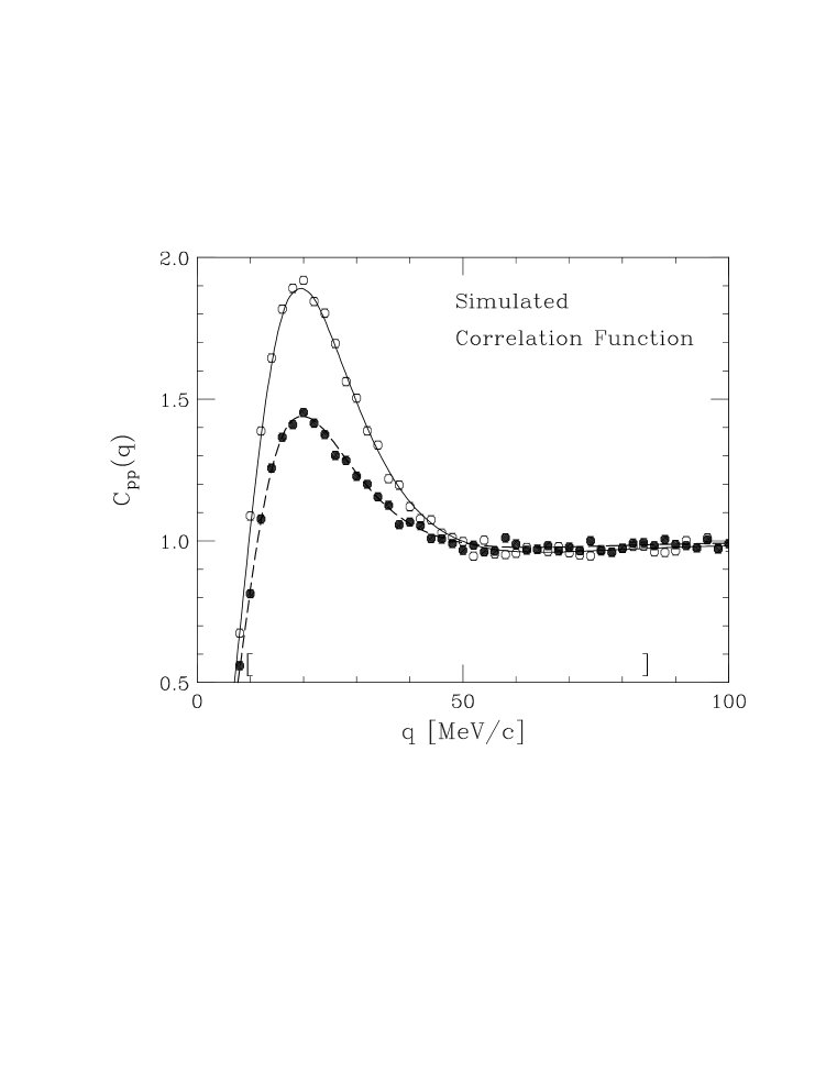
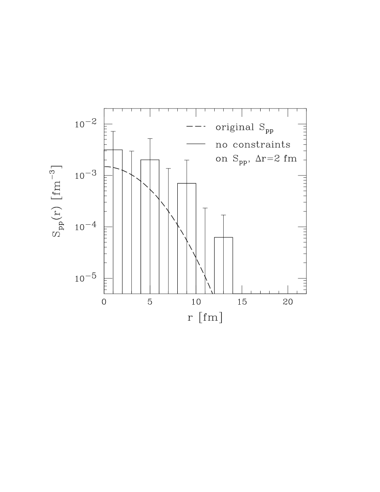
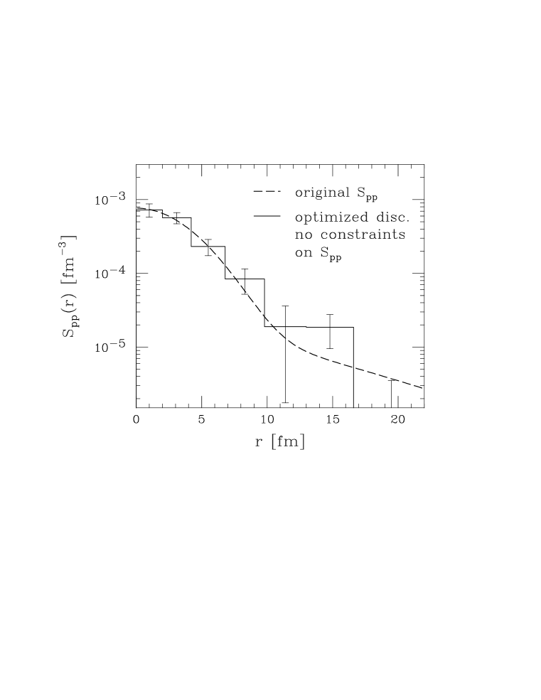
and generate a correlation function $C$ at relative momenta $q$ separated by $\Delta q=2$ MeV/c. We use the folding (3) with the wavefunctions in the kernel calculated by solving the Schrödinger equation with the regularized Reid soft-core potential REID93 [22]. This simulated source is shown in Fig. 1. We take $R_{0}=3.5$ fm in the source and we add random Gaussian-distributed errors to the correlation function from the folding. The rms magnitude of the error is 0.015, which is representative of the pp data of Ref. [15] analysed in [1]. We then attempt to restore the source by discretizing it with 7 intervals of fixed size, $\Delta r=2$ fm, for $r=(0-14)$ fm. We use a $q$–interval similar to the one used in Ref. [1], i.e. $10$ MeV/c $<q<86$ MeV/c. (Note that a naive Fourier-transform argument suggests that a number larger than 7 of $r$-intervals narrower than 2 fm could be used in the inversion.) Results from the restoration according to Eqs. (12) and (13) are shown in Fig. 2, together with the original source function (16). Clearly the errors for restored source far exceed the original source function. In fact, every second value of the restored source is negative. Incidentally, this is one of our more fortunate simulations, since all of the errors actually fit on the logarithmic plot.

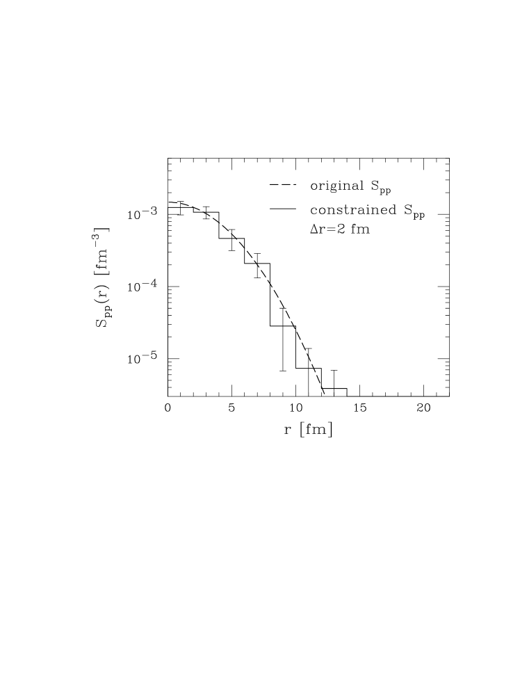
We next illustrate the dramatic stabilizing effect that the constraints have on the imaging, as it was first discussed by Tikhonov [12]. We carry out the inversion using the same correlation function and errors that we used for Fig. 2 (see Fig. 1). We impose the constraints that the imaged source is positive definite, i.e. $S_{j}\geq 0$, as expected in the semiclassical limit, and that the source is normalized: within the restored region $1\geq 4\pi\int_{0}^{r_{N}}dr\,r^{2}\,S\approx 4\pi\sum_{j=1}^{N}S_{j}\int_{r_{j-1}}^{r_{j}}dr\,r^{2}$. Following the general strategies [23] for estimating values with errors and under constraints, we carry out our imaging by sampling the values of the correlation of function according to the errors $\{\sigma_{i}\}_{i=1,\ldots,N}$ (equal to 0.015 in our case) and by applying (12). This amounts to the replacements in (12): $C_{i}\rightarrow C_{i}+\sigma_{i}\,\xi_{i}$, $i=1,\ldots,N$, with $\xi$’s drawn from the standard normal distribution. We accept only those samplings where the constraints are met. With these samplings, we calculate the average source values and the average dispersions. The results are shown in Fig. 3 together with the original source. They now compare favorably to the original source.

In the maximum entropy method [7], as we stated, the constraint of positive source definiteness is implicit. Another constraint one might use [12, 10, 21] is an assumption of smoothness of the source, permitting inversion with more points in the image then there are in the data. Cutting off the integral in the Fourier-transform method [1] at $q_{\rm max}$ implies the constraining assumption that $S$ varies slowly on the scale of $1/(2q_{\rm max})\approx 1.2$ fm in [1], which is reasonable given the range of strong interactions. Finally we comment that, in imaging terms, the common Gaussian parametrization of sources in heavy-ion collisions is a very extreme constraint for stabilizing the inversion.

IV Optimized Discretization

While imposing constraints on the source may stabilize the inversion, we have developed an imaging method that can yield very satisfactory results even without any constraints. Indeed, one may want to see directly whether the data are consistent with positive definite sources. The essential step is to vary the size of the $r$–intervals to minimize relative error of the source.

Thus, the first stage of analysis involves the values of relative momenta $\{q_{i}\}_{i=1,\ldots,M}$, where correlation function was measured, and errors on these measurements $\{\sigma_{i}\}_{i=1,\ldots,M}$, but not the values themselves $\{C_{i}\}_{i=1,\ldots,M}$. Specifically, we vary the edges of the intervals for source discretization, $\{r_{j}\}_{i=1,\ldots,N}$, demanding that the sum of errors relative to some “model source” is minimized at fixed $N$ and $r_{0}=0$,

$$\sum_{j=1}^{N}\left|{\Delta S_{j}\over S^{\rm mod}_{j}}\right|={\rm min}\,,$$ (17)

where the $\{\Delta S_{j}\}_{j=1,\ldots,N}$ are the square roots of the $\{\Delta^{2}S_{j}\}_{j=1,\ldots,N}$ in Eq. (15). We find a rather weak sensitivity of the results to fine details of $S^{\rm mod}$ in (17), so we just use a simple exponential form $S^{\rm mod}\propto\exp{(-r/R_{0}^{\prime})}$, $S^{\rm mod}_{j}=S^{\rm mod}((r_{j-1}+r_{j})/2)$, with $R_{0}^{\prime}$ of the order of few fm. The exponential form is consistent with a possible tail in the source due to prolonged decays.

Features of the squared wavefunction in (2) and the binning in q appear to have the greatest affect on determining the best set $\{r_{j}\}_{i=1,\ldots,N}\,$. Nevertheless, it is important to use relative errors, with some sensible $S^{\rm mod}$, in (17). If absolute errors are taken, then the $r^{2}$ weight from angle-averaging in (8) favors large $r$’s. The net result is that we learn that the source is close to zero at large $r$ to a very high accuracy; we do not need imaging to tell us this. Our practical observation is that the sum of relative errors in (17), rather than the sum of squares, is preferred for minimization; the sum of squares pushes $\{r_{j}\}_{i=1,\ldots,N}\,$inwards, leaving little resolution at high $r$.

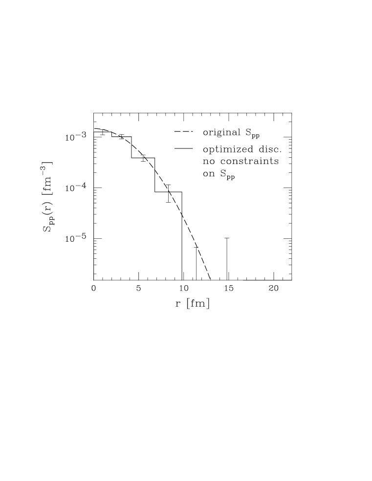
Once an optimal set of $\{r_{j}\}_{i=1,\ldots,N}\,$is found, Eq. (12) can be used to determine the source. The results of applying our procedure to the simulated pp correlation function of the preceeding section, are shown in Fig. 4, for $N=7$. The optimal intervals for discretization typically increase in size with $r$. For example, the first interval in Fig. 4 is 2 fm wide and the sixth is 3.6 fm wide. The figure clearly shows that we can satisfactorily restore the source without imposing any constraints. Figure 5 shows the results from a similar restoration of the source with an exponential tail:

$$S(r)={1\over 2}\,{1\over(2\pi R_{0}^{2})^{3/2}}\exp{\left(-\,{r^{2}\over 2R_{0}^{2}}\right)}+{1\over 2}\,{15\over 4\pi^{5}R_{1}^{4}}\,{r\over\exp{(r/R_{1})}-1}\,,\\$$ (18)

where $R_{0}=3.5$ fm and $R_{1}=6$ fm. We show the correlation function corresponding to the restored source in Fig. (1), both with and without errors of the rms magnitude of 0.015. Since the same $N$ and the same $\{q_{i},\sigma_{i}\}_{i=1,\ldots,M}$ are used in the inversion, we find the same optimal $\{r_{j}\}_{i=1,\ldots,N}\,$used in Fig. 4. The restored source gives evidence for the tail in the source, despite of the fact that the magnitude of the tail is lower by 2 orders of magnitude compared to the maximum at $r=0$. Comparing figures 4 and 5, we see that our method can discriminate between the two source shapes. If we impose additional constraints to the optimized discretization method, the agreement between the restored and original source functions further improves.

V Sources from pp Data

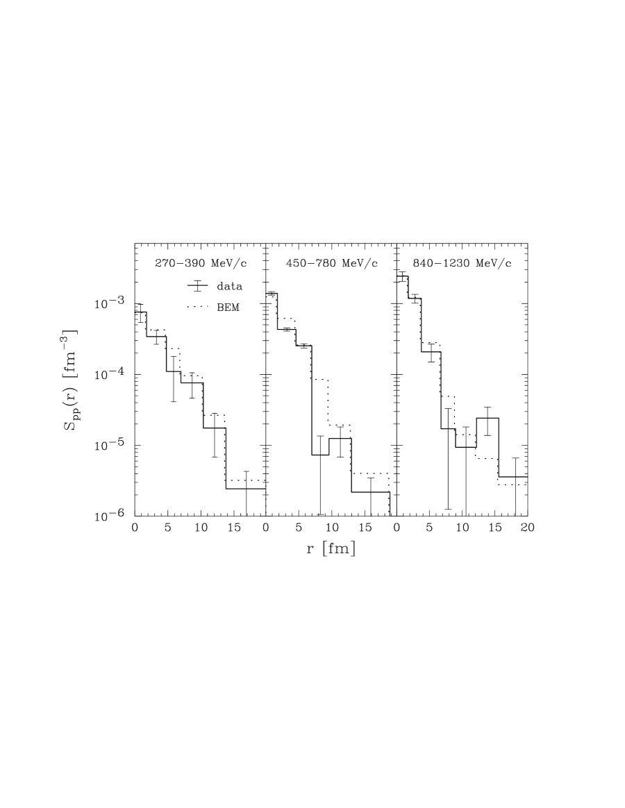
Now we apply our new optimized discretization method to analyse the pp correlation data [15, 16], from the ¹⁴N + ²⁷Al reaction at 75 MeV/nucleon, imaged in the naive fashion in Ref. [1]. Since our new method does not require positive definiteness for stabilization, we are able to lift this constraint and verify whether the data favor positive definite sources. Further, we do need to normalize the sources to 1 within the imaged region. We also compare the pp sources from data to those from the transport model [17], over a large range of relative separations and magnitude of the sources. Past experiences in comparing semiclassical transport models to single-particle and correlation data have been mixed [15, 16, 24, 25, 26] for this particular reaction and others in this energy range.

The low relative-momentum pp-correlations have been determined in Ref. [15, 16] for pairs emitted around $\theta_{\rm lab}=25^{\circ}$ from the ¹⁴N + ²⁷Al reaction at 75 MeV/nucleon, in three intervals of the total momentum: 270–390, 450–780, and 840–1230 MeV/c. The highest lab momenta interval corresponds to the highest proton momenta in the participant cm for this reaction. These momenta are higher than the average for participant protons and directed rather forward. Transport calculations [1, 17] show that the highest momenta bin is mostly populated by pairs from the semicentral to peripheral collisions. The intermediate momenta interval corresponds to the magnitude of typical momenta of participant nucleons in the forward NN cm hemisphere. The transport calculations show that these pairs stem mainly from the semicentral collisions. The lowest lab momenta interval has both participant and target spectator contributions. In the latter case, the transport calculations show that pairs are mostly from the semicentral to central collisions. According to the transport model, the average emission times for protons, from the first contact of the nuclei, in the three momenta intervals, from the highest to lowest, are $\sim 35$, $\sim 80$, and $\sim 110$ fm/c, respectively.

The results of analyzing data using the optimized discretization method are presented in Table I. While we quote only the values obtained using wavefunctions for the REID93 potential, the values for the NIJM2 [22] differ only by a fraction of $1/1000^{\rm th}$. Both the results with and without the positivity and normalization constraints are listed in the table. The results are similar, given their errors. The results obtained without constraints are generally consistent with positive definite source functions. Only in the highest total-momentum interval there might be some indication of a negative minimum in the source function. One can also see in Table I that the magnitude of $S$ in the low-$r$ region increases by a factor of 2 each time one switches from a lower to a higher total-momentum interval.

In Fig. 6, we compare the constrained results from the data to the distributions of relative separation of last collision points for protons with similar momentum from the transport model [1, 17]. Clearly, the semiclassical model can only yield positive-definite source functions. Again, we can see the focussing of the experimental distribution at low $r$ as the pair momentum increases. The large-$r$ tails in the distribution at different momenta cannot be accommodated with the Gaussian parametrizations used to describe the low-$r$ behavior of the sources [15, 16].

Generally (Fig. 6), the Boltzmann-equation model (BEM) yields relative emission point distributions that are similar to the imaged data, including the dependence on total pair momentum. In fact, the maximae around $q=20$ Mev/c (such as in Fig. 1 of the present paper) are nearly the same height as the data (see Fig. 2 in [24]). Such findings are somewhat surprising for the low and intermediate total momentum intervals. While BEM adequately describes high-momentum wide-angle single-particle spectra of protons, which correspond to the highest total-momentum interval (see Fig. 1 in [24]), the model overestimates the single-particle proton spectra by as much as 1.5–5 in the two lower momentum intervals [24]. Looking closer at Fig. 6, we find that the distributions from data are somewhat sharper at low-$r$ in the two lower total-momentum intervals than the the distributions from the model. In the next section, we reveal a serious discrepancy when we go beyond a point by point examination.

VI Generalized Chaoticity Parameter

An important quantity characterizing the imaged distribution can be the integral of the source over a region where the distribution is significant. We introduce the parameter

$$\lambda(r_{N})=\int_{r<r_{N}}d{\bf r}\,S({\bf r})\,.$$ (19)

that generalizes the the chaoticity $\lambda$ used to parametrize high-energy $\pi\pi$ correlations. The term ’chaoticity’ stems from early models involving classical currents used to describe $\pi$ production. The standard chaoticity parameter is defined by fitting the $\pi\pi$ correlation function to a Gaussian:

$$C(q)-1={2\pi\over q}\int_{0}^{\infty}dr\,r\sin{\left(2qr\right)}S(r)\simeq\lambda\exp{\left(-\,{2q^{2}R_{0}^{2}}\right)}\,.$$ (20)

When one uses this parametrization of the correlation function, one assumes the following parametrization of the source at low $r$:

$$S(r)\approx{\lambda\over(2\pi R_{0}^{2})^{3/2}}\exp{\left(-\,{r^{2}\over 2R_{0}^{2}}\right)}.$$ (21)

Our chaoticity parameter generalizes the one in (20) and (21) in two ways. First, because our chaoticity parameter is defined in terms of the imaged source function, rather than a Gaussian fit to the correlation function, it can apply to any particle pair, not just pion pairs. Second it is dependent on the cut–off, $r_{N}$. The importance of our definition of the generalized chaoticity parameter lies in the fact that some particles in the reaction, such as pions or protons, can stem from long-lived resonances and be emitted far from any other particles. Thus, they contribute primarily to $S$ at large $r$, possibly outside the region that may be imaged. If the kernel $K$ is close to zero or averages out to zero for moderate to high $q$ and large $r$, then the tail in $S$ does not contribute to the deviations of $C$ from 1 in Eq. (1) or (20). The imaged region is limited to $r_{N}$ and may result in $\lambda<1$. Access to $C$ at lower $q$ may give higher $r_{N}$ and $\lambda$ closer to 1. However, given experimental limitations on measuring $C$ at the lowest relative $q$, we only really stand a chance to study large $r$ with charged particles (and the higher the charge the better). The charged particles with low relative $q$ should be emitted far apart, otherwise they acquire relative kinetic energy due to mutual repulsion. For the analysed pp data [15], the low-$q$ region is either not available or is associated with large systematic errors. Imaging can only extend up to $r_{N}\sim 20$ fm. Thus, one can expect $\lambda(r_{N})<1$. In many $\pi\pi$ measurements, e.g. [28], the resolution allows one to image [1] regions of comparable sizes, typically 10–20 fm. In contrast to the $pp$ and $\pi\pi$ data, the data on IMF (such as [18]) often extend to low values of relative velocity because of the use of fragments with large charges. This permits imaging up to relative separations as large as 50 fm. For a discussion of this, see the next section.

In Table II, we have tabulated $\lambda(r_{N})$ in each momentum interval for the constrained and unconstrained sources of Section III as well as sources from the BEM. Comparing the results of the BEM to the constrained source, we only find agreement in the highest momentum interval. It follows that, when compared to the model, significant portions of the source are missing from the imaged regions. This discrepancy is especially pronounced in the intermediate-momentum region. Nevertheless, it is comforting that the transport model describes the features of the relative source for the high momentum protons since it properly describes [24] the high-momentum single-particle spectra. Now, in BEM no IMFs are produced and the IMFs may decay over an extended time, contributing to large separations in the relative emission function, as they move away from the reaction region. Of course these decays produce some final IMFs, contributing to the relative IMF sources at distances similar to those for the pp sources. It may be interesting to see whether a significant portion of the relative IMF sources can extend beyond $\sim 20$ fm, as is apparent for the pp sources. We check this in the next section of the paper.

The disagreements between the data and calculations in both the values of $\lambda(r_{N})$ and the single-particle spectra [24], for the lower momenta, reveal unphysical features of low-momentum proton emission in the transport model. The coarse agreement between the measured correlation function and the function calculated using the model in Ref. [24] in the lower total-momentum intervals, mentioned in the last section, is coincidental. Since the images show $\lambda(r_{N})<1$, some of the strength of $S$ is shifted out to large $r$ lowering the height of $C$. For BEM, the height of $C$ is lowered because $S$ is softer than $S$ from the data. Thus, the BEM correlation function can match the height of the measured correlation peak, while not matching the overall shape of the correlation function. For other systems in the general energy range, disagreements were found even in the height of $C$ [16, 25, 26].

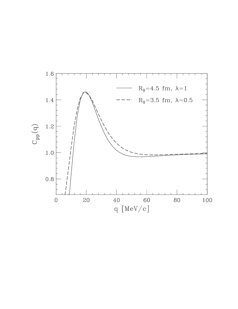
These conclusions raise the question of the general sensibility of attempting to fit the magnitude of pp or nn correlation function at the maximum [29, 15, 16] by adjusting the radius $R_{0}$ in the Gaussian parametrization of the source function (see Eq. (21)) with $\lambda=1$. When fitting the $\pi\pi$ correlation functions at intermediate relative momenta, both the strength and extent of the source function at low $r$ are varied: $\lambda$ is read off from the magnitude of the correlation function at low $q$ and $R_{0}$ is read off from the width of the correlation function in $q$. However, because of the resonant nature of the low-momentum NN interaction, the height of the NN correlation function is determined by the magnitude of the source within the resonance peak of the wavefunction. That magnitude is both affected by the overall low-$r$ strength of the source and the low-$r$ source falloff. This is illustrated in Fig. 7 which shows pp correlation functions for the source (21): the same maximum height can be obtained using $R_{0}=4.5$ fm and $\lambda=1$ as using $R_{0}=3.5$ fm and $\lambda=0.5$.

Given that the resonance peak in the ${}^{1}S_{0}$ wavefunction is quite narrow (it has an outer radius of $\sim 2.5$ fm) and the source falloff cuts off large-$r$ contributions to the integration in (1), the low-$r$ limit of $S$ is proportional to the $C-1$ at the maximum (to a $\pm 20\%$ level) for virtually all low-$r$ falloffs that may be encountered in practice, $R_{0}=2.5-6.0$ fm:

$$C_{\bf P}(20\,{\rm MeV/c})\approx 1+540\,{\rm fm^{3}}\,S_{\bf P}(r\rightarrow 0).$$ (22)

For the two sources we used in Fig. 7, we get about the same value of $S(r\rightarrow 0)$ and therefore about the same maximum height in $C$. With the same maximum height, the source falloff is reflected in the width of the maximum in Fig. 7. Note that the value of $S$ at short relative distances determines the average freeze-out phase-space density and the entropy in the reactions [32, 1]; the simple relation for estimating the proton phase-space density takes the form, from (22),

$$\langle f({\bf p})\rangle=0.0018\,\left({{\rm GeV}\over c}\right)^{3}\,(C_{2{\bf p}}^{\rm max}-1)\,{E_{p}\over m}\,{dN_{p}\over d{\bf p}}\,,$$ (23)

where $dN_{p}/d{\bf p}$ is the proton momentum distribution.

VII IMF Sources

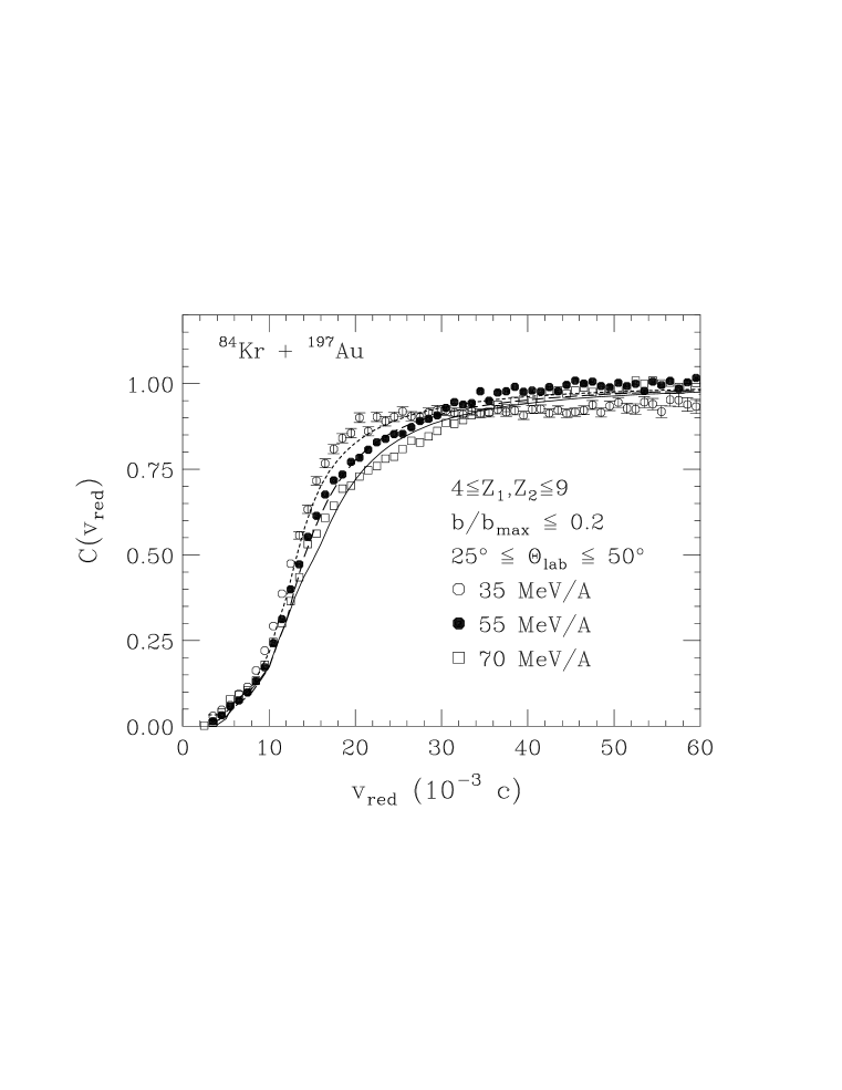
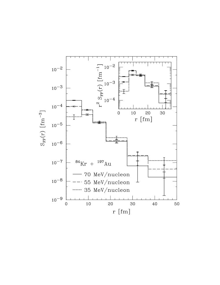
We now turn to the analysis of IMF sources. We choose the correlation data of Hamilton et al.  [18], from central ⁸⁴Kr + ¹⁹⁷Au reactions at 35, 55, and 70 MeV/nucleon, because these data give us the opportunity to examine the variation of sources with beam energy.

Pairs were collected in the angular range of $25^{\circ}<\theta_{\rm lab}<50^{\circ}$ in order to limit contributions to the correlation functions in [18] from targetlike residues. Hamilton et al. determine the functions in terms of the reduced velocity

$$v_{\rm red}={v\over(Z_{1}+Z_{2})^{1/2}}\,,$$ (24)

under the assumptions that the Coulomb correlation dominated the fragment correlation and that the fragments were approximately symmetric, $Z/A\approx 1/2$. The distance of closest approach in (6) for symmetric fragments is

$$r_{c}={2\,Z_{1}\,Z_{2}\,(A_{1}+A_{2})\,e^{2}\over A_{1}\,A_{2}\,m_{N}\,v^{2}}={e^{2}\over m_{N}\,v_{\rm red}^{2}}\,.$$ (25)

The correlation functions at the three beam energies are shown in Fig. 8. We have reduced the normalization for the correlation function at 35 MeV/nucleon by 5%, compared to [18], in order to better satisfy the condition that $C\rightarrow 1$ at large $v_{\rm red}$, outside of the region shown in Fig. 8. In examining Eqs. (1), (6), (25), and Fig. 8, certain issues become apparent. Contributions to the Coulomb correlation function $C$ for a given $v_{\rm red}$ stem only from the region of the source with $r>r_{c}$. As $v_{\rm red}$ increases from 0, the distance of closest approach $r_{c}$ decreases, with more and more inner regions of the source $S$ contributing to $C$. The low-$v_{\rm red}$ correlation functions at the three beam energies in Fig. 8 are quite similar, suggesting that the tails of the source functions are similar. Differences occur at higher $v_{\rm red}$, indicating differences in the inner source regions.

To image of the IMF sources, we optimize $\{r_{j}\}_{i=1,\ldots,N}\,$as in the pp case, but we add the constraint $r_{1}\geq r_{1}^{\rm min}$. We do this because the Coulomb interaction in (1) does not dominate when the measured fragments are in close contact. The Coulomb correlation alone cannot be relied upon to get information on the most inner portion of the source. The typical touching distance for the fragments measured in [18] is $r_{t}\sim 5$ fm; we chose a value $r_{1}^{\rm min}=7.0$ fm which ensures that there is more volume in the lowest bin outside $r_{t}$, than inside $r_{t}$.

The results from the imaging are shown in Fig. 9. Given the errors in the figure, the tails of the sources at the three energies are not very different. However, we observe significant variation with energy at short relative distances ($r<12$ fm) with the source undergoing a larger change between 55 and 75 MeV/nucleon, than between 35 and 55 MeV/nucleon.

In Table III we tabulate the generalized chaoticity parameter for the IMF sources with the cutoff of 20 fm and over the whole restored image. The values of $\lambda$ for the whole image (cutoff of 90 fm) are all consistent with 1, within errors. The values of $\lambda$(20 fm) 20–30% below 1 and Fig. 9 indicate that a large part of IMF emission occurs at distances that are not imaged with protons. Nevertheless, the values of $\lambda(\sim$20 fm) the low- and high-momentum pp sources in Section V are roughly equal to the IMF $\lambda$(20 fm) but the intermediate-momentum pp $\lambda$(20 fm) is lower. It should be mentioned that no complete quantitative agreement should be expected, even if the data were from the same reaction and pertained to the same particle-velocity range. This is because more protons than IMFs can stem from secondary decays. Besides, the velocity gained by a proton in a typical decay is large compared to the relevant relative velocities in pp correlations, but the velocity gained by an IMF can be quite small on the scale of velocities relevant for the IMF Coulomb correlations. Thus, the IMF correlations may reflect the primary parent sources, which are concentrated around the origin, rather than the final sources.

The tails of the IMF sources extend so far that they must be associated with the time extension of emission. Even so, it is interesting to ask how far into the center of the source must we go to see the effects due to the spatial extent of the primary source. In [18], the combinations of single-particle source radii and lifetimes that gave acceptable descriptions of their data have radii varying between 5 and 12 fm. In general, the combination of spatial extent and lifetime effects should give rise to a bone-like shape of the relative source, with the source elongation being due to the emission lifetime. With this, one could try to separate the temporal and spatial effects by restoring the full a three-dimensional source. In the angle-averaged source, the part dominated by lifetime effects should fall off as an exponential divided by the square of the separation, $r^{2}$, as a function of relative separation. On the other hand, the part of the relative source dominated by spatial effects may fall off at a slower pace or even be constant. In Fig. 9, we see that the sources change weakly with $r$ at 35 and 55 MeV/nucleon and faster at 70 MeV/nucleon, within the range where sources vary with energy ($r$  $\raisebox{-2.15277pt}{$\stackrel{{\scriptstyle<}}{{\scriptstyle\sim}}$$\,\,$}12$ fm). For reference, in the insert to Fig. 9 we show the IMF source multiplied by $r^{2}$. We see an edge at $r\sim 11$ fm at 35 and at 55 MeV/nucleon which disappears at 70 MeV/nucleon, suggesting that the IMF’s are emitted from a spatial region, with a radius $R\sim 11/\sqrt{2}\sim 8$ fm, that becomes more dilute as the energy increases. This observation is consistant with the expectation that dilute sources are more effective at emitting IMF’s since IMF yields in central symmetric collisions or from central sources in asymmetric collisions maximize towards 100 MeV/nucleon [30].

VIII Conclusions

We have introduced the new method of optimized discretization to image sources. This method is suitable for determining the relative source from different particle pair correlations in heavy-ion collisions. Recognizing the need for stable imaging, in our method we adjust the resolution to minimize the relative errors of the source. The fact that we can actually estimate errors in this method gives our method a significant advantage over the maximum entropy method. We tested our method by restoring assumed compact pp sources and found that the quality of the restored source is comparable to the restored source we obtain by imposing the constraints of positivity and normalization. Imposing these constraints in our new method further reduces the source errors, but imposing these constraints is no longer required. The new method allows one to study the long-range source structure by adjusting the overall size of the imaged region and the resolution at large distances.

The robustness of our new imaging method gave us the capability to examine the positive definiteness of proton Wigner sources in the ¹⁴N + ²⁷Al reaction at 75 MeV/nucleon [15, 16]. In principle, unraveling the quantal negative values of a Wigner function is not far fetched. In fact, negative values of Wigner functions have been observed in interfering atomic beams [31]. Admittedly, if we had discovered such values in the heavy-ion reactions, we would first have to check for a possible breakdown of the assumptions leading to (1) and on systematic errors in data, before concluding on a success. The extensive averaging in the reactions makes it unlikely that a genuinely quantal oscillation in the source function would survive except in the very tail of the function.

We found that our imaged sources change significantly with the total pair momentum, becoming sharpest for the largest momenta in the cm. Significant portions of the imaged source are missing from the imaged region at typical participant momenta in the cm, but not at the highest momenta. The chaoticity parameter (the integral of the source) from the Boltzmann-equation model [27, 17] agrees with the data at the highest momenta, but the integral is close to one in the participant and target-emission momenta. Nevertheless, the model yields the correct height of the maximae of the correlation functions [24]. This is because the right combination of source normalization and sharpness in the model can yield the right value of $S$ at short separations, $S_{\bf P}(r\rightarrow 0)$, and this primarily determines the height of $C$. Gaussian-source fits to the height of the pp correlation function [29, 15, 16] are of a limited value because considerable source strength may lie at large relative separations.

In our analysis of midrapidity IMF sources in central ⁸⁴Kr + ¹⁹⁷Au reactions at different beam energies, we found a significant variation of the sources with energy at short distances, but not at large distances. Considerable portions of the IMF sources extend to large distances ($r>20$ fm) just like the lower total-momentum pp sources. It would be very interesting to image both the IMF and pp sources in one reaction. There is a deficiency of our fragmentation analysis method, namely our method lacks three-body Coulomb effects. When weak, these effects could be included as a first-order perturbation.

As this work was nearing completion, it was suggested [33] that we use nested Gaussians, of variable width and centered at $r=0$, in place of sharp-edged intervals in our source description. The Gaussians would generalize nicely to three dimensions while maintaining the features of the error optimization in our method and we will investigate the possibility of using them in the near future. Our strategy of letting the errors and the kernel choose what source they can image is novel not just for the problem of inverting correlations but the inversion problem in general [7].

TABLE I.: Relative pp source values restored from the data of Ref. [15] through the optimized discretization method, with ($S^{\rm co}$) and without ($S^{\rm nc}$) constraints imposed for three total momentum gates. The centers of the discretization intervals are $r_{k-1/2}=(r_{k}+r_{k-1})/2$ and the size is $\Delta r_{k}=r_{k}-r_{k-1}$. The number of intervals is either $N=6$ (two lower momentum gates) or $N=7$ (the highest gate).

$P$-Range	k	$r_{k-1/2}$	$10^{4}\times S_{k}^{\rm nc}$		$10^{4}\times S_{k}^{\rm co}$		$\Delta r_{k}$
[MeV/c]		$[{\rm fm}]$	$[\mbox{fm}^{-3}]$		$[\mbox{fm}^{-3}]$		[fm]
	1	$0.9$	7.6$\pm$	2.2	7.6$\pm$	2.2	$1.8$
	2	$3.3$	3.55$\pm$	0.90	3.42$\pm$	0.76	$3.0$
	3	$5.9$	1.07$\pm$	0.91	1.10$\pm$	0.69	$2.2$
270–390	4	$8.7$	0.85$\pm$	0.34	0.76$\pm$	0.30	$3.4$
	5	$12.1$	0.30$\pm$	0.21	0.18$\pm$	0.11	$3.4$
	6	$16.9$	–0.024$\pm$	0.047	0.024$\pm$	0.019	$6.2$
	1	$0.9$	13.89$\pm$	0.70	13.87$\pm$	0.69	$1.8$
	2	$3.2$	4.18$\pm$	0.24	4.30$\pm$	0.21	$2.8$
	3	$5.8$	2.69$\pm$	0.22	2.54$\pm$	0.17	$2.4$
450–780	4	$8.3$	–0.10$\pm$	0.13	0.073$\pm$	0.063	$2.6$
	5	$11.3$	0.161$\pm$	0.075	0.124$\pm$	0.057	$3.4$
	6	$15.9$	0.017$\pm$	0.018	0.022$\pm$	0.013	$5.8$
	1	$0.9$	25.0$\pm$	4.5	24.3$\pm$	3.7	$1.8$
	2	$2.8$	9.8$\pm$	2.3	11.8$\pm$	1.7	$2.0$
	3	$5.3$	2.89$\pm$	0.98	2.09$\pm$	0.59	$3.0$
840–1230	4	$7.9$	–1.08$\pm$	0.88	0.17$\pm$	0.16	$2.2$
	5	$10.6$	–0.20$\pm$	0.38	0.094$\pm$	0.088	$3.2$
	6	$13.9$	0.41$\pm$	0.22	0.24$\pm$	0.10	$3.4$
	7	$18.2$	0.009$\pm$	0.089	0.036$\pm$	0.030	$5.2$

TABLE II.: Comparison of the integral of the relative pp source function, $\lambda(r_{N})$, for the restored and BEM sources in three total momentum gates in the ¹⁴N + ²⁷Al reaction at 75 MeV/nucleon. The restored sources use the data of Ref. [15]. The integrals are truncated at the distance $r_{N}$.

$P$-Range	$\lambda(r_{N})$					$r_{N}$
[MeV/c]	unconstrained		constrained		BEM	[fm]
270-390	0.69$\pm$	0.22	0.69$\pm$	0.15	$0.98$	$20.0$
450-780	0.560$\pm$	0.065	0.574$\pm$	0.053	$0.91$	$18.8$
840-1230	0.65$\pm$	0.37	0.87$\pm$	0.14	$0.88$	$20.8$

TABLE III.: Comparison of the integrals of the midrapidity IMF source function, $\lambda(r_{N})$, in central ⁸⁴Kr + ¹⁹⁷Au reactions at three beam energies, for different truncation points, $r_{N}$. The restored sources use the data of Ref. [18].

Beam Energy	$\lambda(90\,{\rm fm})$		$\lambda(20\,{\rm fm})$
[MeV/nucleon]
35	0.96$\pm$	0.07	0.72$\pm$	0.04
55	0.97$\pm$	0.06	0.78$\pm$	0.03
70	0.99$\pm$	0.05	0.79$\pm$	0.03

FIG. 1.: The solid line is the correlation function from the source in Eq. (16) and the dashed line is from the source in Eq. (18). We obtained the wavefunctions in the kernel in (3) by solving the Schrödinger equation with the REID93 potential [22]. The symbols are the values of the correlation functions with added random errors of rms magnitude 0.015. The square brackets above the horizontal axis indicate the range of $q$ we used to restore source.

FIG. 2.: The solid histogram is the relative pp source function $S$ restored from the simulated correlation function in Fig. 1 indicated there by the open symbols. The dashed line is the original source function in (16) that we used to generate the correlation function. We employed fixed-size intervals of $\Delta r=2$ fm for discretizing the source function and we imposed no constraints on $S$.

FIG. 3.: This plot is the same as Fig. 2, except that the restored source is constrained to be positive and its integral is restricted to be less than one.

FIG. 4.: This plot is the same as Figs. 2 and 3, except that the source is not constrained and is restored with the optimized discretization method.

FIG. 5.: The solid histogram is the relative pp source restored using the optimized discretization method. The correlation function used is indicated by the filled circles in Fig. 1. The original source function is shown with the dashed line.

FIG. 6.: Relative source for protons emitted from the ¹⁴N + ²⁷Al reaction at 75 MeV/nucleon, in the vicinity of $\theta_{\rm lab}=25^{\circ}$, in the three total momentum intervals of 270–390 MeV/c (left panel), 450–780 MeV/c (center panel), and 840–1230 MeV/c (right panel). Solid lines are the source values extracted from the data [16] and the dotted lines are the source values obtained in the Boltzmann-equation calculation.

FIG. 7.: The solid line is the two-proton correlation function for $R_{0}=4.5$ fm and $\lambda=1$ while the dashed line is for $R_{0}=3.5$ fm and $\lambda=0.5$. The source is the Gaussian in Eq. (21).

FIG. 8.: Fragment-fragment velocity correlation function in central ⁸⁴Kr + ¹⁹⁷Au reactions. The symbols show the data of Ref. [18] and the lines show the imaged source function. The 35 MeV/nucleon data is represented by the open circles and dotted line, the 55 MeV/nucleon data by solid circles and dashed line, and 70 MeV/nucleon by open squares and solid line.

FIG. 9.: Relative source for IMFs emitted from central ⁸⁴Kr + ¹⁹⁷Au reactions from the data of Ref. [18] at 35 (dotted line), 55 (dashed line), and 70 MeV/nucleon (solid line). The insert shows the source multiplied by $r^{2}$. In both plots, the full image extends out to $90$ fm.