Testing the Core-Halo Model
on Bose-Einstein Correlation Functions

1 Introduction

High energy heavy ion collisions are providing a reproducible experimental environment to study physics at extremely high energy densities in relatively large volumes. A tool to access the space-time characteristics of such systems is the technique known as intensity interferometry. If the observed particles are bosons, intensity interferometry is frequently referred to as HBT effect [1] or Bose-Einstein correlations [2, 3, 4]. These intensity correlations appear due to the enhanced (decreased) likelihood that a boson (fermion) is produced in a quantal state that is close in phase-space to a state already occupied by another boson (fermion). Intensity interferometry is a fastly developing tool for studying spatial and temporal extension of hot and dense strongly interacting systems on the $10^{-15}$ m and $10^{-23}$ s scales.

Accumulating evidence indicates, that high energy heavy ion reactions, performed currently at CERN SPS and Brookhaven AGS, create composite sources of particles, that can be approximately divided into two parts: a central core, where the time evolution of the matter can be thought as a violent cascading of binary collisions or hydrodynamical behavior of strongly interacting matter, and a halo of long-lived resonances, that are created in the hot and dense medium but decay far outside the core. In case of pions, the resonance halo undoubtedly contains the decays of $K_{S}^{0}$ where $\tau=8.9\cdot 10^{-9}$ s, the decays of the $\eta$ and $\eta^{\prime}$ resonances that have a very narrow decay widths of $\Gamma_{\eta}=1.20$ keV and $\Gamma_{\eta^{\prime}}=0.2MeV$. The lifetimes of these resonances correspond to $\tau=\hbar/\Gamma=164417$ fm/c and 986.5 fm/c, respectively. The next long-lived resonance which is expected to be produced in significant numbers in high energy collisions is the $\omega$ meson with a full width of $\Gamma_{\omega}=8.4$ MeV and a corresponding life-time of $\tau_{\omega}=23.4$ fm/c. In the literature, one may observe a scientific debate weather the decay products of the $\omega$ mesons contribute to the halo or not.

After a brief summary of the statements made about the contribution of the omega resonance to the BECF-s, we attempt to conclude this debate in case of the $S+Pb\rightarrow\pi+\pi+X$ reaction measured by the NA44 Collaboration at CERN SPS [5], by presenting an analysis of this data set along the lines suggested in ref. [6]. In case of other reactions or other experimental resolutions/techniques, we emphasize that the role of the $\omega$ meson should be investigated again, in a manner similar to the analysis presented in the forthcoming sections.

The main purpose of the present paper is to test, whether the core/halo model interpretation of the two-particle correlation function is indeed applicable to the above cited NA44 data, or not, with the help of a novel method suggested in ref. [6]. If the core/halo interpretation of the measured correlation function is meaningful, the parameterization of the correlation data should be independent of the data points at the lowest values of the relative momentum, hence these data points could be deleted without significantly changing the fitted parameters of the correlation functions. We check the validity of this hypothesis by gradually removing the data points at smallest relative momentum from the NA44 $S+Pb$ data set. To our best knowledge, this is the first time that such kind of analysis is performed on measured correlation data, in order to verify the applicability of the core/halo model. Hence, we must establish the limits of the technique to be used before attempting the data analysis.

The paper is structured as follows: In Section 2 we summarize the basics of Bose-Einstein correlations and the assumptions that are introduced to obtain the core/halo model. We also summarize here those various theoretical considerations and conclusions about the influence of the $\omega$ meson on the two-pion correlation function, that were achieved in earlier numerical investigations, reviewing the status of this scientific debate.

In Section 3, we describe a Monte-Carlo procedure that was used to estimate the limits of the procedure that we utilized to verify the applicability of the core/halo picture to NA44 data in the subsequent Section 4. Finally, we summarize and conclude. Conceptually, our study is also related to a recently discussed “model-independent” Gaussian parameterization of the correlation functions. In Appendix A we evaluate the Gaussian model-independent radii in the core/halo model and compare the resulting “model-independent” correlation functions to the prediction of the core-halo model. Then we give a re-formulation of the “model-independent” parameterization of the correlation functions that can be applied to core/halo type of models as well as systems without halo and clarify the model assumptions that have to be made in order to achieve this “model-independent” result.

In the followings, we use natural units, $\hbar=c=1$, to simplify the notation.

2 Correlation Functions and the $\omega$-Puzzle

Let us briefly recapitulate the theoretical description of the two-particle Bose-Einstein correlation functions following the lines of refs. [6, 7].

Particle emission is characterized by the single-particle Wigner-function $S(x,p)$. Here $x=(t,{\bf r}\,)$ denotes a point in space-time and $p=(E,{\bf p}\,)$ a point in momentum-space. The emitted particles are on mass-shell, $m=\sqrt{E^{2}-{\bf p}^{\,2}}$.

An auxiliary quantity can be introduced as

$$\tilde{S}(\Delta k,K) = \int d^{4}x\,\,S(x,K)\,\exp(i\Delta k\cdot x),$$ (1)

where $\Delta k=p_{1}-p_{2}$, $K={(p_{1}+p_{2})/2}$ and $\Delta k\cdot x$ denotes an inner product.

The invariant momentum distribution can be expressed as

$$E{\displaystyle\phantom{|}dn\over\displaystyle\phantom{|}d{\bf p}} = N_{1}({\bf p})\,=\,\tilde{S}(\Delta k=0,K=p).$$ (2)

In the present paper, we utilize the so called hydrodynamical normalization of the Wigner-functions,

$$\int{\displaystyle\phantom{|}d{\bf p}\over\displaystyle\phantom{|}E}d^{4}xS(x,p) = \int{\displaystyle\phantom{|}d{\bf p}\over\displaystyle\phantom{|}E}N_{1}({\bf p})\,\,=\,\,\langle n\rangle,$$ (3)

where $\langle n\rangle$ is the mean multiplicity.

The two-particle correlation function can be written as

$$C_{2}({\bf p}_{1},{\bf p}_{2}) = {\displaystyle\phantom{|}N_{2}({\bf p}_{1},{\bf p}_{2})\over\displaystyle\phantom{|}N_{1}({\bf p}_{1})\,N_{1}({\bf p}_{2})}\,=\,1+{\displaystyle\mid\tilde{S}({\bf\Delta k},{\bf K})\mid^{2}\over\displaystyle\phantom{|}\tilde{S}(0,{\bf p}_{1})\tilde{S}(0,{\bf p}_{2})}\,\simeq\,1+{\displaystyle\mid\tilde{S}({\bf\Delta k},{\bf K})\mid^{2}\over\displaystyle\phantom{|}\mid\tilde{S}(0,{\bf K})\mid^{2}},$$ (4)

e.g. in ref. [8, 9]. Interestingly, this formalism can be introduced not only when multi-particle symmetrizations are negligible, but even when they are fully taken into account [10]. For the most recent derivation, where full multi-particle symmetrization effects were included, see ref.  [10].

The last approximation in eq. (4) can be estimated to give correct results within 5 % error  [11]. We have neglected here final state interactions, and a completely chaotic particle emission is assumed.

The second and the higher order Bose-Einstein correlation functions,

$$C_{n}({\bf p}_{1},{\bf p}_{2},...,{\bf p}_{n}) = {\displaystyle\phantom{|}N_{n}({\bf p}_{1},{\bf p}_{2},...,{\bf p}_{n})\over\displaystyle\phantom{|}N_{1}({\bf p}_{1})N_{1}({\bf p}_{2})...N_{1}({\bf p}_{n})}$$ (5)

are given [12] in terms of the Fourier-transformed Wigner-functions as

$$C_{n}({\bf p}_{1},{\bf p}_{2},...,{\bf p}_{n}) = {\displaystyle\phantom{|}\sum_{\sigma^{n}}\prod_{i=1}^{n}\tilde{S}(i,\sigma_{i})\over\displaystyle\phantom{|}\prod_{i=1}^{n}\tilde{S}(i,i)}\,\,=\,\,\sum_{\sigma^{n}}\prod_{i=1}^{n}{\displaystyle\phantom{|}\tilde{S}(i,\sigma_{i})\over\displaystyle\phantom{|}\tilde{S}(i,i)}\,\,=\,\,\sum_{\sigma^{n}}\prod_{i=1}^{n}\tilde{s}(i,\sigma_{i}),$$ (6)

where $\sigma^{n}$ stands for the set of permutations of $n$ indexes,

$$\tilde{S}(i,\sigma_{i})\,=\,\tilde{S}({\bf K}_{i,\sigma_{i}},{\bf\Delta k}_{i,\sigma_{i}}), \tilde{s}(i,\sigma_{i})\,=\,{\displaystyle\phantom{|}\tilde{S}(i,\sigma_{i})\over\displaystyle\phantom{|}\tilde{S}(i,i)},$$ and (7)

$${\bf K}_{i,\sigma_{i}}\,=\,{\displaystyle\phantom{|}{\bf p}_{i}+{\bf p}_{\sigma_{i}}\over\displaystyle\phantom{|}2}, {\bf\Delta k}_{i,\sigma_{i}}\,=\,{\bf p}_{i}-{\bf p}_{\sigma_{i}}.$$ and (8)

Note the difference between $\sigma^{n}$, which stands for a set of permutations and $\sigma_{i}$ (subscript $i$), which stands for the permuted value of index $i$ in a given permutation from the set $\sigma^{n}$.

Let us recapitulate the Assumptions of the core/halo model from ref.  [7]:

Assumption 0: The emission function does not have a no-scale, power-law like structure. This possibility was discussed and related to intermittency in ref. [13].

Assumption 1: The bosons are emitted either from a central part or from the surrounding halo. Their emission functions are indicated by $S_{c}(x,p)$ and $S_{h}(x,p)$, respectively. According to this assumption, the complete emission function can be written as

$$S(x,p)=S_{c}(x,p)+S_{h}(x,p),$$ (9)

using the hydrodynamic normalization of the Wigner functions.

Assumption 2: We assume that the emission function which characterizes the halo changes on a scale $R_{H}$ which is larger than $R_{max}\approx\hbar/Q_{min}$, the maximum length-scale resolvable [6] by the intensity interferometry microscope. However, the smaller central part of size $R_{c}$ is assumed to be resolvable, $R_{H}>R_{max}>R_{c}$. This inequality is assumed to be satisfied by all characteristic scales in the halo and in the central part, e.g. in case the side, out or longitudinal components [14, 15] of the correlation function are not identical.

Assumption 3: The momentum-dependent core fraction $f_{c}(i)=N_{c}({\bf p}_{i})/N_{1}({\bf p}_{i})$ varies slowly on the relative momentum scale given by the correlator of the core $\tilde{s}_{c}(1,2)\tilde{s}_{c}(2,1)$.

Let us also recapitulate the normalization conditions:

$$\int d^{4}x{\displaystyle\phantom{|}d{\bf p}\over\displaystyle\phantom{|}E}S_{c}(x,p)\,=\,\langle n\rangle_{c}, \int d^{4}x{\displaystyle\phantom{|}d{\bf p}\over\displaystyle\phantom{|}E}S_{h}(x,p)\,=\,\langle n\rangle_{h},$$ and (10)

where the subscripts $c,h$ refer to the contribution from the central core and from the halo, respectively.

Note that ref [6] also utilized the above Assumptions, however, in a modified form, that was based on Wigner-functions normalized to 1, and a core-fraction $f_{c}=\langle n\rangle_{c}/\langle n\rangle$ was introduced, while in the present paper a momentum-dependent core fraction $f_{c}({\bf p})=N_{c}({\bf p})/N({\bf p})$ is utilized. One finds that

$$N_{1}({\bf p})\,=\,N_{c}({\bf p})+N_{h}({\bf p}), \langle n\rangle\,=\,\langle n\rangle_{c}+\langle n\rangle_{h}.$$ and (11)

According to ref.  [7], the general expression for $C_{n}(1,...,n)$ reads in the core/halo model as

$$C_{n}(1,...,n) = 1+\sum_{j=2}^{n}\sum_{i_{1},...,i_{j}=1}^{\hbox{}\,\,\,n\,\,\,_{\prime}}\sum_{\rho^{n}}\prod_{k=1}^{j}f_{c}(i_{k})\tilde{s}_{c}(i_{k},i_{\rho_{k}}).$$ (12)

where $\sum^{\prime}$ refers to a summation over different values of the indices (i.e. $i_{j}=i_{k}$ type of terms are excluded). For the two-particle correlation function, the above equation takes a particularly simple form:

$$C_{2}(1,2) = 1+f_{c}(1)f_{c}(2)\tilde{s}_{c}(1,2)\tilde{s}_{c}(2,1).$$ (13)

With the help of Assumption 3, the core/halo model thus predicts the following form for the two-particle correlation function:

$${C({\bf\Delta k}_{12},{\bf K}_{12})} = 1+\lambda_{*}({\bf K}_{12}){\displaystyle\phantom{|}\mid\tilde{S}_{c}({\bf\Delta k}_{12},{\bf K}_{12})\mid^{2}\over\displaystyle\phantom{|}\tilde{S}_{c}(0,{\bf p}_{1})\tilde{S}_{c}(0,{\bf p}_{2})},\,\simeq\,1+\lambda_{*}({\bf K}_{12}){\displaystyle\phantom{|}\mid\tilde{S}_{c}({\bf\Delta k}_{12},{\bf K}_{12})\mid^{2}\over\displaystyle\phantom{|}|\tilde{S}_{c}(0,{\bf K}_{12})|^{2}},$$

where one introduces an effective intercept parameter as

$$\lambda_{*}({\bf K})=\left[N_{c}({\bf K})/N_{1}({\bf K})\right]^{2}.$$ (15)

As emphasized in Ref. [6], this effective intercept parameter ( which is not the same as the exact intercept parameter, $\lambda_{x}=1$ at $Q=0$ MeV) shall in general depend on the mean momentum of the observed boson pair, which within the errors of $Q_{min}$ coincides with any of the on-shell four-momentum $p_{1}$ or $p_{2}$.

Thus one obtains the core/halo interpretation of the two-particle correlation function:

The measured part of the BECF picks up an effective, momentum dependent intercept parameter $\lambda_{*}({\bf K})$, that depends on the mean momentum only and which can be used as a tool to measure the momentum dependence of the fraction of particles that are emitted from the core. On the other hand, the relative momentum dependence of the BECF-s carries the information on the core in this picture. Note, that in high energy heavy ion collisions the momentum dependence of the $\lambda_{*}({\bf K})$ parameter is very weak, actually, within the errors $\lambda_{*}({\bf K})$ is constant for the NA44 data analyzed in ref. [6]. However, the validity of Assumption 3 has to be checked experimentally for each data set, by determining the momentum dependence of the $\lambda({\bf K})$ parameter of the two-particle correlation function.

At this point, we emphasize that non-Gaussian correlation functions with $0\leq\lambda_{*}\leq 1$ are very well possible within the core/halo picture, as discussed e.g. in refs. [6, 16]. We shall discuss in Appendix A under what conditions can the core correlator have an approximate Gaussian shape.

Since the core-halo model neglects possible partial coherence, motivated by the success of fully chaotic Monte-Carlo simulations of high energy heavy ion collisions like RQMD [17], the exact intercept parameter is $\lambda_{x}=1$ and the value of the exact intercept of the two-particle correlation function is always $1+\lambda_{x}=2$ in the core/halo picture. The effect of long-lived resonances is to create an unresolvable, narrow peak in the region $0<Q<Q_{min}$ from the interference of the particles of $(h,h)$ and $(h,c)$ type, i.e. from those pairs which have at least one member of the pair from the core. This is illustrated in Figure  1, taken from Ref. [6].

Another very important general observation is that the region with small $Q$ has a different characteristic structure from that of $Q>Q_{min}$ region. Thus any analytical expansions of the Bose-Einstein correlation functions around the $Q=0$ point become both qualitatively and quantitatively unreliable for the core-halo type of systems, characterized by $0<\lambda_{*}<1$. This point is further elaborated in the Appendix, let us return now to the detailed discussion of the core-halo model using an example.

Note, that in principle the core as well as the halo part of the emission function could be decomposed into more detailed contributions. We shall argue below, that in case of $S+Pb$ reactions at 200 AGeV at CERN SPS, in the NA44 acceptance, one can separate the contribution of various long-lived resonances as

$$S_{h}(x,p)\,=\,\sum_{r=\omega,\eta,\eta^{\prime},K^{0}_{S}}S^{(r)}_{h}(x,p) N_{h}({\bf p})\,=\,\sum_{r=\omega,\eta,\eta^{\prime},K^{0}_{S}}N^{(r)}_{h}({\bf p}).$$ and (16)

For a general consideration, e.g. the ones discussed in ref. [7], the question whether the $\omega$ decay products contribute to the halo or not, is essentially indifferent. However, when a data analysis is performed, this question becomes important both qualitatively and quantitatively, influence of the $\omega$ meson on the shape and the intercept parameters of the two-particle correlation functions is suggested in various theoretical papers, see e.g. refs. [15, 17, 18, 19, 20, 21, 22, 23].

Let us briefly summarize the various statements made in this scientific debate. Essentially, three different type of statements were made regarding the influence of decay products of the $\omega$ meson on the short range part of the two-particle correlation function. Although we cannot repeat the fine-prints and all the reservations that were made in earlier papers on this point, we think that a rough (and probably incomplete) summary can be made as follows:

A

The effect of the $\omega$ decay products is clearly visible on the two-particle BECF. These decay products are mainly responsible for the deviation of the BECF from a Gaussian shape and they influence the intercept parameter also in a non-trivial manner. Essentially, the $\omega$ decays contribute to the resolvable, core part of the source.

B

The decay products of the $\omega$ meson should be considered as an intermediate case. Their contribution should be partially visible, resulting in a deviation from the Gaussian shape of the BECF.

C

At the current level of experimental techniques, $Q_{min}\approx 5-10$ MeV and $B(Q)_{max}\geq 25$ MeV, the $\omega$ decay products can be taken as part of the halo. Their contribution to the two-particle BECF cannot be resolved experimentally in case of NA44 data.

In the core/halo picture, the points A - C correspond to the following conclusions: In case of A, the $\omega$ decay products belong to the core. In case of B, the core/halo model is not applicable to simplify the theoretical treatment of the two-particle BECF-s. This case corresponds to a really complicated situation. Finally, in case of C, the $\omega$ decay products contribute to the halo and the theoretical description of the correlation function can be simplified substantially.

Let us also give a (probably incomplete) list of papers where these statements were made. Conclusion A has been reached in ref. [15], in a Monte-Carlo simulation with the help of SPACER, and later in ref. [21] assuming $5$ MeV $Q_{min}$ resolution for $Pb+Pb$ reactions at CERN SPS in a 3d hydrodynamical simulation with the code HYLANDER. Conclusion B was reached in refs. [20, 22, 23, 24], using phenomenological parameterization of a hydrodynamically evolving core with thermally populated resonance production. In all these studies, full resonance decay kinematics was included and resonance production was described either in a thermal manner or in a non-equilibrium process with the help of re-scattering. All of these studies share in common that they evaluated the correlation function as a mathematical function but they did not consider in detail the error bar distribution on the theoretical curve.

Finally, in refs. [6, 7, 25, 26], conclusion C was reached based on considerations related to the NA44 detector resolution and the surprisingly Gaussian shape of the measured NA44 correlation functions.

Another interesting study was performed recently by Padula and Gyulassy [27], that included a simulation of binning and detector resolution effects for AGS energies with the help of the inside-outside cascade code CERES, with proper resonance decay kinematics, to conclude that

D Preliminary data seem to rule out dynamical models with significant $\omega$ and $\eta$ resonance fraction yields in case of the E802 measurement of $Si+Au$ data at 14.6 AGeV at Brookhaven AGS.

We do restrict our study to CERN SPS reactions, and published NA44 data. In the next section, we perform a Monte-Carlo simulation to make a connection between source parameters and the parameters of the fitted correlation functions before attempting the data analysis.

3 Monte Carlo Simulations

For the sake of simplicity, one may simplify the problem by fixing the mean momentum of the observed particle pairs and introduce the source density for those particles which are emitted with the given mean momentum as $\rho_{\bf K}(x)=S(x,\mathbf{K})$. The index ${\bf K}$ will thus be suppressed in the forthcoming, but implicitly we shall assume that the analysis is performed at a fixed value of $\mathbf{K}$. Also, in the applications, we shall analyze NA44 data where the mean momentum of the pairs is restricted to a certain range. We have had access only to the one dimensional slices of a three-dimensional NA44 data set, along the main axis in the LCMS frame [15]. These data were taken at a fixed mean momentum. In effect, we thus analyzed three different one dimensional data set instead of analyzing a single three dimensional one. As the quality of the published data is expected to be improved in the near future, we hope that this limitation will disappear and in a future analysis one may study the 3d correlation functions at a fixed value of ${\bf K}$ directly in a similar manner as presented below.

The limitation that we had access to 1d slices of data yields an advantage as well, since it is enough for the present paper to formulate the procedure for one dimensional distributions only. The generalization of the method for multi-dimensional distributions is trivial hence it will be omitted.

In the core/halo picture, the source density is written as

$$\rho(x)=f_{c}\rho_{c}(x)+(1-f_{c})\rho_{h}(x)$$ (17)

where $f_{c}$ from now on represents the fraction of pions produced in the core at the given mean momentum $\mathbf{K}$. In order to make predictions for the model, forms for $\rho_{c}(x)$ and $\rho_{h}(x)$ must be assumed. With Gaussian assumptions for both, $\rho_{i}(x)=\frac{1}{\sqrt{2\pi R_{i}}}e^{-x^{2}/2R_{i}^{2}}$, the resulting correlation function is

$$C_{2}(Q)=1+f_{c}^{2}e^{-R_{c}^{2}Q^{2}}+(1-f_{c})^{2}e^{-R_{h}^{2}Q^{2}}+2f_{c}(1-f_{c})e^{-\frac{1}{2}(R_{c}^{2}+R_{h}^{2})Q^{2}}$$ (18)

Examination of this expression reveals Gaussian terms for the core, the halo, and an ‘interference’ term. Figure 2 shows the relative size of these terms, as a function of some momentum variable $Q$, for typical values of $f_{c}$, $R_{c}$, and $R_{h}$. The effect of the halo is to introduce a sharp peak in the correlation function at low values of $Q$. This narrow peak in $Q$-space is indicative of a large length-scale in $x$-space. Note that the model predicts $C_{2}(Q=0)=2$ – there is no need to assume any coherent boson production which would reduce the intercept. Figure 3 illustrates the effect of the $f_{c}$ parameter on the correlation function.

Since we are more interested in the radius parameters of the core than the halo, the easiest way to extract the proper core parameters is to remove the low $Q$ data points so that the effect of the halo is negligible, a procedure suggested e.g. in ref. [6]. This simple method minimizes the effect of the Gaussian assumption for the shape of the halo structure - as long as the length-scale of the halo is large compared to $\hbar/Q_{min}$, removing the low $Q$ points should remove the halo’s effects. Fitting the remaining data with a standard Gaussian form should produce $R=R_{c}$ and $\lambda=f_{c}^{2}$.

However, given the finite experimental resolution of $\sim$10 MeV/c, the halo may not be visible at all. If this is the case, the extracted $\lambda$ and $R$ parameters still have an interpretation as the fraction of core pions (squared) and the core radius parameter, respectively. If they do not change as $Q_{min}$, the minimum value of $Q$ included in the data, is increased, it will indicate that the correlation function really is Gaussian. This would contradict the prediction that some resonances distort the Gaussian shape of the correlation function.

In either case, we must establish the limits of the procedure before attempting the analysis of real data. There must be some maximum number of data points that can be removed from a real correlation function while still being able to extract valid parameters. If that number is too small, then the idea of removing low $Q$ points in order to study the correlation function of the core is invalid - if the length-scales of the core and the halo cannot be separated, then the fitted parameters of the truncated correlation function become dependent on $Q_{min}$, the size of the excluded region.

The core-halo model takes advantage of finite experimental resolution – as resolution increases, and more of the low $Q$ structure of $C_{2}(Q)$ is revealed, perhaps a more detailed model will be necessary. But for now, this reasonable model imitates the effects of resonance production and can attribute physical significance to the $R$ and $\lambda$ parameters extracted from a correlation function.

3.1 The acceptance-rejection method

What is required is a method of producing correlation functions where the underlying parameters are known in advance, so they can be compared to the extracted parameters. This will be done by simulating the actual distribution $A(Q)$ and the background distribution $B(Q)$ that a real experiment uses to produce $C_{2}(Q)=A(Q)/B(Q)$.

It is necessary to assume a form for $A(Q)$ and $B(Q)$ in order to do this. The background distribution $B(Q)$ is different for every experiment, so one must parameterize it appropriately each time. The $A(Q)$ distribution will not be parameterized directly; rather, we will assume a form for $C_{2}(Q)$, and then simulate the distribution $A(Q)=B(Q)\cdot C_{2}(Q)$. In this way, we can have control over the parameters that are going into the simulation. The finite number of iterations performed in the simulation ensure that these parent distributions are never reproduced exactly, so the assumed form for $C_{2}(Q)$ is not returned directly. Binning effects are automatically included and, most importantly, the error-bar distribution on the correlation function will follow the experimental one at least when statistical errors are considered. Fits shall be done with optimizing $\chi^{2}/NDF$ hence the error bar distribution plays an important role when determining the best fitted values and their errors.

We would like to emphasize that the simulation of the $A(Q)$ and $B(Q)$ distributions is essential when discussing possible resonance effects on the two-particle correlation function, since the resonance decay products are expected to influence the shape of the Bose-Einstein correlation function in the $Q\leq 50$ MeV region [15, 19, 6, 22, 23] and they also contribute to the fitted value of the radius and the intercept parameters. However, the fitted values are strongly influenced by the distribution of the errors on the data points, since the fit selects to reproduce the best that part of the correlation function, which has the smallest errors. Unfortunately, very few experiments decided to publish their actual and background distributions, but some [28, 29, 30, 31, 5] did this important step. Even fewer theoretical models tried to reproduce the distribution of the statistical errors on the data as arising from the number of actual and background pairs as a function of the relative momentum. In fact, none of the theoretical simulations that reached a conclusion belonging to type A or B included this important step.

Unfortunately, it is not possible to sample from the complicated distributions $A(Q)$ and $B(Q)$ directly. Instead, we will use the acceptance-rejection method, which works as follows: Let the known distribution to be sampled be denoted by $p(Q)$, that will be chosen as $A(Q)$ or $B(Q)$ in the subsequent parts. The probability distribution $p(Q)$ should be normalized, $\int p(Q)\,dQ=1$, over the range of interest. Find a comparison function, $f(Q)$, which has the following properties:

1. Let $f(Q)$ satisfy $f(Q)>p(Q)$ for all $Q$.

2. There exists a closed form for a random $Q$ point sampled from $f(Q)$.

In the interest of computational efficiency, the comparison function $f(Q)$ should be chosen to be as close to $p(Q)$ as possible, while still satisfying $f(Q)>p(Q)$, in order to minimize the number of rejected points. A random $Q$ point, $Q_{i}$, is sampled from the comparison function $f(Q)$. Then the value of the parent distribution $p(Q_{i})$ is calculated. The ratio $R=p(Q_{i})/f(Q_{i})$, which is always less than 1, is then compared to another uniform random number $U^{\prime}$. If $U^{\prime}>R$, the point $x_{i}$ is rejected and the process starts over again. If $U^{\prime}<R$, $Q_{i}$ is accepted. In this way, the distribution $p(Q)$ is sampled.

3.2 Simulating a one dimensional correlation function

If we assume the halo form for $C_{2}(Q)$, eq. 18, the two distributions to be simulated are $B(Q)$ and $A(Q)$. For the CERN experiment NA44, studying S+Pb collisions, the shape of $B(Q)$ is given approximately by [32]

$$B(Q)=Q^{3}e^{-3.6Q^{0.3}},$$ (19)

hence the $A(Q)$ distribution is sampled as

$$A(Q)=B(Q)(1+f_{c}^{2}e^{-R_{c}^{2}Q^{2}}+(1-f_{c})^{2}e^{-R_{h}^{2}Q^{2}}+2f_{c}(1-f_{c})e^{-\frac{1}{2}(R_{c}^{2}+R_{h}^{2})Q^{2}}).$$ (20)

For these one-dimensional simulations, $Q$ can be any relative momentum variable – $Q_{inv}$, $Q_{side}$, $Q_{out}$, etc. The above expression for $B(Q)$ was given for $Q_{inv}$, but it is valid for any one dimension of $\mathbf{Q}$ as long as the other components are small. The parameters for a Lorentzian comparison function are adjusted by hand until the Lorentzian satisfies condition 1) reasonably well. The Lorentzian comparison function was sampled as suggested in ref. [33]. With the help of Lorentzian comparison functions, the distributions $A(Q)$ and $B(Q)$ were sampled as described above. As each point was sampled from either $A(Q)$ or $B(Q)$, it is binned. The bin size of 10 MeV/c is chosen to reflect experimental situation for the multi-dimensional NA44 data analysis. The value of $Q$ for each bin is calculated by averaging all entries, from both $A(Q)$ and $B(Q)$, that fall in that bin. Figure 4 shows the results of the simulations of $A(Q)$, $B(Q)$, and the resulting $C_{2}(Q)$. The number of iterations for the simulation is chosen to give reasonable error bars on the final $C_{2}(Q)$. The number of iterations must be higher for $A(Q)$, however, since $A(Q)>B(Q)$ for all $Q$. The areas under the curves are used to calculate the proper ratio of iterations.

The error bars are calculated as follows. For $A(Q)$ and $B(Q)$, we assume that the number of entries in each bin is Poisson distributed, so that the error for each bin is just the square root of the number of bin entries. The errors for $C_{2}(Q)$ are then just combined in the usual manner.

Now we can fit the simulated correlation function with a standard Gaussian shape, $C_{2}(Q)=1+\lambda e^{-R^{2}Q^{2}}$, reflecting experimental analysis techniques, and observe the behavior of the parameters as $Q_{min}$ is increased. Figure 5 shows the value of the $R_{*}$ and $\lambda_{*}$ parameters as low $Q$ data points are removed. The solid lines represent the input values, $R_{c}=4.0$ fm and $f_{c}^{2}=0.5625$. Examining these results indicates that reliable values for the parameters can be extracted, i.e. $R_{*}=R_{c}$ within errors and $\lambda_{*}=f_{c}^{2}$ within errors, when $Q_{min}$ is varied in the range of 10 to 50 MeV/c. We can also read off from Figure  5 that the fitted radius and intercept values are essentially insensitive to the exact value of $Q_{min}$ if this is varied in the above range.

4 Core/halo model analysis of NA44 data

We now apply the data chopping analysis, tested in the earlier section, to real experimental data. CERN experiment NA44 has been running since 1991, and has an extensive collection of correlation function data [29, 30, 34, 35, 31, 5]. We analyze their S+Pb data. The data set is three-dimensional – that is, it covers all of the (out, side, long) space, but we only have access to slices of the data along the three axes. So in effect we are analyzing three one-dimensional slices of the three-dimensional Bose-Einstein correlation functions, for each published data set. Values of the two-particle correlation functions and their errors were read directly off the published figures by eye, as accurately as possible. NA44 has analyzed S+Pb data for both $\pi^{+}$ and $K^{+}$. The $\pi^{+}$ data were taken with two different magnetic settings – ‘high $p_{t}$’ data is characterized by $<p_{t}>=450MeV/c$, and the ‘low $p_{t}$’ data has $<p_{t}>=150MeV/c$. This was done in an attempt to observe some detailed dynamics of the system.

Thus we have analyzed the slices of the three-dimensional NA44 Bose-Einstein correlation function for the low-$p_{t}$ and high-$p_{t}$ pion sample and for the kaon sample in $S+Pb$ reactions at CERN SPS, data were from refs. [5, 37]. Unfortunately, we had no access to the three-dimensional distributions either for NA44 measurements or for other data. Ideally, the analysis presented below should have been performed on the (unpublished) three-dimensional distributions. However, our final result indicates that the extracted values for the intercept parameters are within errors similar for each projection of the NA44 sample, which justifies the utilization of the projections in this particular case.

Our analysis results are shown in the Figures  6-11. Note that the left-most data point in each figure represents the value of that particular parameter when none of the data points are removed. Also, with three separate slices along the three main axis instead of one three-dimensional set, one can extract three values for the $\lambda$ parameter. The NA44 analysis produces just one $\lambda$, since they fit to

$$C_{2}(Q)=1+\lambda e^{-Q_{out}^{2}R_{out}^{2}-Q_{side}^{2}R_{side}^{2}-Q_{long}^{2}R_{long}^{2}}$$ (21)

The parameters show no significant, systematic change as $Q_{min}$ is increased. This confirms that the shape of the correlation function really is Gaussian. In the context of the core-halo model, this suggests that long-lived resonances are not resolved by NA44, neither in case of pions, nor for kaons, see Figures (6-11).

In order to extract values for $R$ and $f_{c}$ from this analysis, we fit the previous data with a constant (see Table  1). The data up to $Q_{min}=40$ MeV/c are chosen, since this has been shown to be a reliable range.

parameter	high $p_{t}$ $\pi^{+}$	low $p_{t}$ $\pi^{+}$	$K^{+}$
$R_{c\ out}$ (fm)	2.92 $\pm$ .13	4.29 $\pm$ .13	2.54 $\pm$ .18
$R_{c\ side}$ (fm)	2.90 $\pm$ .18	4.24 $\pm$ .26	2.22 $\pm$ .19
$R_{c\ long}$ (fm)	3.31 $\pm$ .16	5.43 $\pm$ .30	2.67 $\pm$ .22
$f_{c\ out}$	.704 $\pm$ .012	.725 $\pm$ .011	.802 $\pm$ .027
$f_{c\ side}$	.735 $\pm$ .021	.647 $\pm$ .021	.736 $\pm$ .033
$f_{c\ long}$	.738 $\pm$ .014	.724 $\pm$ .015	.789 $\pm$ .029

Table 1: Extracted values for $R_{c}$ and $f_{c}$ from NA44 S+Pb data.

These results show several things. As expected, the kaon core fraction is larger than either pion fraction. Further, the trend in the core radii is $R_{kaon}<R_{highp_{t}}<R_{lowp_{t}}$. The interpretation of this result is not a trivial task [16]. One would first imagine that the decrease of these radii follows the trend of increasing resonance influence, suggesting that short-lived resonances can also affect core radii. It is also possible that kaons decouple from the interaction region sooner than pions do. Secondly, the core fractions are similar for the high and low $p_{t}$ data, since the intercept parameter is within errors independent of the transversal mass of the particles. One might argue that the constancy of the $\lambda$ parameter implies that any increase in resonance contribution in the low $p_{t}$ data takes place in the short-lived resonances.

Name	$m$ (MeV)	$\tau$	Decay	$f_{Fritiof}$	$f_{RQMD}$
direct $\pi$	140	7.804 m	-	0.19	0.33
$\rho$	770	1.3 fm	$\pi\pi$	0.40	0.26
$\Delta$	1232	1.64 fm	$N\pi$	0.06	0.12
$K^{*}$	892	3.94 fm	$K\pi$	0.09	0.07
$\Sigma(1385)$	1385	5.5 fm	$\Sigma\pi$	0.01	0.02
$\omega$	783	23.4 fm	$\pi\pi\pi$	0.16	0.07
$\eta\prime$	958	982 fm	$\eta\pi\pi$	0.02	0.02
$\eta$	548	$1.64\times 10^{5}$ fm	$\pi\pi\pi$	0.04	0.03
$K_{S}^{0}$	498	2.7 cm	$\pi\pi$	0.03	0.07

Table 2: Sources of pions in relativistic heavy ion collisions, taken from Ref. [20].

This interpretation, however, is not likely since hydrodynamical expansion may also result in a strong transversal mass dependence of the measured radius parameters [16], even an approximate $m_{t}$ scaling can be obtained in this manner in a certain limiting case. Further, a comparison of Tables 1 and  2 indicates that the measured core fractions are in the vicinity of the core fractions of Fritiof and RQMD if $\omega$, $\eta$ and $\eta^{\prime}$ are taken as unresolved long lived resonances, as indicated by Table  3.

$f_{c,NA44}$ (high $p_{t}$ $\pi^{+}$ )	$f_{c,NA44}$ (low $p_{t}$ $\pi^{+}$ )	$f_{c,Fritiof}$	$f_{c,RQMD}$
0.71 $\pm$ 0.01	0.71 $\pm$ 0.01	0.75	0.80

Table 3: Core fractions $f_{c}$ from NA44 S+Pb data compared to core fractions from RQMD and Fritiof, when $\omega$, $\eta$ and $\eta^{\prime}$ are taken as unresolved long-lived resonances. The core fractions for the NA44 low $p_{t}$ and high $p_{t}$ sample are obtained from a simultaneous fit to ($f_{c,out},f_{c,side},f_{c,long}$) by a constant value, and the result is rounded to two decimal digits.

Since both $\omega$ and $\eta$ decay predominantly into three pions, in a narrow region of phase space characterized by $m-3m_{\pi}$, these resonance decays should produce predominantly low-$p_{t}$ pions. Similar conclusion holds also for the $\eta^{\prime}$ resonance where the phase space is characterized by $m_{\eta^{\prime}}-2m_{\pi}-m_{\eta}$, which is also rather small. Thus a resonance interpretation of the $m_{t}$ dependence of the radius parameters seems to contradict to the observed constancy of the $\lambda$ parameters. Collective effects, like three dimensional hydrodynamic expansion and $m_{t}$ dependent volume factors that enhance the direct production of pions at low $p_{t}$ as compared to the direct production of heavier resonances were discussed as a possible solution of this puzzle in Refs. [16, 6, 41].

In the future, we hope that this type of analysis will be applied to full three-dimensional data sets by various experimental groups. This would be more significant for several reasons. First, several recent papers [36, 38] have suggested the presence of cross-terms in the 3-D correlation function, something which cannot be detected with just slices of data along the three axes. Secondly, the 1-D slices we have used may cover up some of the low-$Q$ detail, since they integrate over small regions of the other two dimensions (typically $<40$ MeV/c).

Looking farther ahead, the core-halo model could be useful in the next generation of heavy ion experiments. Physicists at RHIC or at CERN experiment NA49 expect to have a $Q$ resolution of $\leq$ 5 $MeV/c$, which could be sufficient to see the halo directly.

5 Conclusions

In summary, an outline of Bose-Einstein correlation analysis for heavy ion collisions has been presented. In contrast to theoretical predictions of a complicated correlation function due to the effect of resonance decays, experimental correlation functions seem to be characterized by just a single intercept parameter $\lambda$ and a set of Gaussian radius parameters, $R_{side}$, $R_{out}$, $R_{long}$ (and $R_{out-long}$). As an attempt to incorporate resonance effects into a simple correlation model, core and resonance halo sources are dealt with separately, each characterized by a Gaussian width parameter along with a core fraction parameter. Data from NA44 do indicate indirectly the presence of such a halo. Our results cast doubt on the validity of predictions that long-lived resonances produce complicated structure in the Bose-Einstein correlation function at CERN SPS, when observed with a two-particle resolution of $Q_{min}\approx 10$ MeV.

In the Appendix, we present one of the simplest possible application of the core-halo model to illustrate that the Gaussian “model independent” HBT radii are unreliable qualitatively and are unreliable quantitatively in their frequently quoted original form, if the intercept parameter $\lambda<1$. At the end of the Appendix, we include the corrected definition of these parameters, that can be applied to core/halo type of systems with $\lambda<1$ also.

Acknowledgments:

T. Csörgő would like to thank to Professors Kiang and Gyulassy for their kind hospitality at Dalhousie and Columbia Universities. This research was supported by the OTKA Grants W01015107, T016206, T024094 and by an Advanced Research Award of the Fulbright Foundation and by an operating grant from the Natural Sciences and Engineering Research Council of Canada.

Appendix A: What do “Model-Independent Radii” measure?

In this Appendix, we discuss the Gaussian model-independent radii of the HBT correlation functions in terms of the core/halo model, along the lines of ref. [39].

Let us recall the definition of the “model-independent” Gaussian radius parameters:

$$R_{i,j}^{2} = \langle(x_{i}-\beta_{i}t)(x_{j}-\beta_{j}t)\rangle-\langle(x_{i}-\beta_{i}t)\rangle\langle(x_{j}-\beta_{j}t)\rangle,$$ (22)

$$C(\mathbf{K},\mathbf{\Delta k}) = 1+\exp\left(-R^{2}_{i,j}Q_{i}Q_{j}\right),$$ (23)

$$N({\bf p}) = \langle 1\rangle,$$ (24)

$$\langle f(x,p)\rangle = \int d^{4}xf(x,p)S(x,p),$$ (25)

where $i=side,out$ or $long$, $\beta_{i}=K_{i}/K_{0}$ is the component of the four-velocity vector of the pair in the direction $i$ and $Q_{i}=\mathbf{\Delta k}_{i}$, and $S(x,p)$ is the emission function that characterizes a chaotic system, see ref. [36, 11].

For clarity, it is better to consider a one-dimensional system only. Let us consider a core/halo type of system, with Gaussian ansatz for both the core and the halo part, with a core radius of $R_{c}=4$ fm, a halo radius of $R_{H}=40$ fm, and a core-fraction is assumed to be $f_{c}=0.75$. Let us compare the full correlation function $C_{2}(Q)$, given by eq. (18) to the core/halo model approximation $C_{2}^{c/h}(Q)$, given as

$$C_{2}^{c/h}(Q) = 1+\lambda_{*}\exp(-R_{*}^{2}Q^{2})$$ (26)

$$\lambda_{*} = f_{c}^{2}\,=\,0.56$$ (27)

$$R_{*} = R_{c}\,=\,4\mbox{\rm~{}fm}$$ (28)

and to the model-independent Gaussian approximation to correlation function, $C_{2}^{G}(Q)$, which reads as

$$C_{2}^{G}(Q) = 1+\lambda_{G}\exp(-R_{G}^{2}Q^{2}),$$ (29)

$$\lambda_{G} = 1\quad\mbox{\rm by definition},$$ (30)

$$R_{G}^{2} = \langle x^{2}\rangle-\langle x\rangle^{2}\qquad\rightarrow\quad R_{G}=20.3\mbox{\rm~{}fm}.$$ (31)

This comparison is visualized in Figure  12.

In Figure  12 it is clearly visible, that the model-independent Gaussian parameterization of the correlation function works only in the $Q<\hbar/R_{h}=5$ MeV region. The variance of the source function is dominated by the variance of the halo part, and this is picked up by the model-independent Gaussian radii. The approximation works in the unobservable $Q$ range, however, in the well measurable $Q>10$ MeV region the resulting correlation function approximates rather incorrectly the full correlation function. On the other hand, the core/halo model approximation fails in the unobservable $Q<5$ MeV region, but it approximates with high accuracy the correlation function in the observable $Q>10$ MeV. If a measurement is performed in the $Q>10$ MeV range, the extrapolated correlation function will be a Gaussian with $\lambda<1$. We may conclude, that for a core/halo type of system, the Gaussian model-independent approximation yields qualitatively incorrect results in the range $Q>\hbar/\langle x\rangle^{2}_{h}$, when naively compared to a measurement of such a correlation function, since $\lambda<1$ will be measured experimentally. If the radius parameter is considered only, its value is quantitatively wrong ($R_{G}=20.3$ fm instead of 4 fm) in the model-independent approximation [36], since $R_{G}^{2}=\langle x^{2}\rangle-\langle x\rangle^{2}$ is dominated by the contribution of the halo.

Note that the authors of refs. [11, 36] warned the readers against the straightforward applications of their result. Let us quote their warning from ref. [11]: “ We would like to point out, that one must take care when comparing the above radii with the experimentally measured correlation radii, since the former measure second derivatives around $Q=0$, while the latter are parameters of a Gaussian fit to the whole correlation function …”.

Such non-Gaussian structures appear e.g. in the case of stable distributions, like the Lorentzian distribution, for which the Fourier-transformed distribution exists, however the first or the second moment of the distribution diverges thus the Fourier-transformed distribution is not analytic at small values of the relative momenta. See appendix of Ref. [16] for further details on this point. Such a non-Gaussian correlation function may characterize even the core part of the distribution.

From the above example it is clear that a direct application of the of the original definitions of the Gaussian model-independent radii, as was proposed originally in refs. [36, 11] leads to qualitatively and quantitatively unreliable results if applied even to very simple models of core-halo type. The Gaussian model-independent radii were obtained in refs. [36, 11] from an expansion around the $Q=0$ point. However, according to Figure  1, in this region the correlation function may have a narrow and unresolved structure, dominated by the large regions of homogeneity in the halo. Obviously, the variances as determined by the above relationships shall be dominated by the variances of the halo part of the system, and in effect one obtains a nice Gaussian approximation to the Bose-Einstein correlation function — in the unresolved range of $Q<Q_{min}\approx 10$ MeV. However, the resolved part of the correlation function shall be missed completely by this approximation. See Figure 12 for an illustration of the effect.

From the above is also quite obvious, how to modify the original definitions of the model-independent radii to get an approximation to the measured correlation functions: the variances should be evaluated for the core emission function only. Although the possibility of such a characterization was discussed in ref. [23, 22] in a manner similar to the present Appendix, the equations corresponding to such a description were not given there. We provide these below, since they may become a practically useful tool to characterize the two-particle Bose-Einstein correlation functions in high energy heavy ion collisions.

This step results e.g. in a hydrodynamical like predictions for these radii and in a $0<\lambda_{*}<1$ intercept parameter of the correlation function. A necessary condition for the applicability of the Gaussian approximation is that the first two moments of the source distributions of the core should be finite. The exceptional stable distributions (e.g. the Lorentzian) do not satisfy this criteria. We know that the mean of the core distribution is always finite hence the criteria is reduced to the requirement that the variances of the core be finite. Under these conditions, the two-particle correlation function in the core/halo picture can be rewritten as

$$C^{c/h}(\mathbf{K},\mathbf{\Delta k}) = 1+\lambda_{*}({\bf K})\,\exp\left(-R^{2}_{i,j}({\bf K}){\bf\Delta k}_{i}{\bf\Delta k}_{j}\right),$$ (32)

$$\lambda_{*}({\bf K}) = [N_{\bf c}({\bf K})/N({\bf K})]^{2},$$ (33)

$$R_{i,j}^{2}({\bf K}) = \langle(x_{i}-{\mathbf{\beta}}_{i}t)(x_{j}-{\mathbf{\beta}}_{j}t)\rangle_{\bf c}-\langle(x_{i}-{\mathbf{\beta}}_{i}t)\rangle_{\bf c}\langle(x_{j}-{\mathbf{\beta}}_{j}t)\rangle_{\bf c},$$ (34)

$$\langle f(x,{\bf p})\rangle_{\bf c} = \int d^{4}xf(x,{\bf p})S_{\bf c}(x,{\bf p}),$$ (35)

where $i=side,out$ or $long$ as before, and $S_{\bf c}(x,{\bf p})$ is the emission function that characterizes the central core. Thus the halo contributes in this model to the reduction of the intercept parameter only and the variances of the core correspond to the Gaussian core/halo model radii of the measured correlation function. This result cannot be obtained with an expansion around $Q=0$, on the other hand, it can be obtained with the help of a moment expansion of the source distribution function around $x=\langle x\rangle_{c}$, which becomes possible if the second moment of the core distribution is finite. Hence, this result corresponds to a large $Q$ expansion of the Bose-Einstein correlation function [40].

Although the above parameterization is a rather straight-forward combination of core - halo model and the expressions for the “model-independent” HBT radii, the results can still be considered simultaneously as a particular Gaussian approximation of the more general core/halo model result of eq. (LABEL:e:lamq) as well as a generalization of the “model-independent” Gaussion HBT radii for systems of core/halo type.

Figure Captions

Fig. 1

Full line indicates the effective, measured correlation function of the core/halo model using Gaussian ansatz for both the halo and the core, $R_{c}=4.0$ fm/c, $R_{H}=40$ fm/c. Dashed line stands for the full correlation function, which includes the effect from the halo, resulting in a narrow and unresolvable peak if $Q_{min}=10$ MeV is the experimental resolution. The extrapolated intercept parameter, $\lambda_{*}$ thus deviates from the exact intercept of $\lambda_{x}=1$, however, $\lambda_{*}$ carries important information about the fraction of core particles at a mean momentum.

Fig. 2

The value of the three terms in the core-halo model correlation function. $f_{c}=0.75,R_{c}=4.0$ fm, $R_{h}=40.$ fm

Fig. 3

The effect of $f_{c}$ on $C_{2}(Q)$ in the core-halo model for $R_{c}=4.0$ fm and $R_{h}=40.$ fm.

Fig. 4

The simulated $A(Q)$ and $B(Q)$ distributions, and the resulting $C_{2}(Q)$. Error bars are too small to be seen for the actual and the background distributions $A(Q)$ and $B(Q)$. Input values were $R_{c}=4.0$ fm, $R_{h}=40.$ fm and $f_{c}=0.75$. To simulate the $A(Q)$ distribution of the pion pairs, 349,476 points were sampled, for the $B(Q)$ distribution, 300,000. Note, that these $A(Q)$ and $B(Q)$ distributions were chosen to peak at 25 MeV, similarly to the CERN experiment NA44.

Fig. 5

The behaviour of the fitted $\lambda_{*}$ and $R$ parameters as low $Q$ data points are removed from $C_{2}(Q)$. Solid line stands for $\lambda_{*}=f_{c}^{2}$ and $R_{fit}=R_{core}$.

Fig. 6

Radius parameters as a function of $Q_{min}$ for NA44’s low $p_{t}$ $\pi^{+}$ data.

Fig. 7

$\lambda_{*}$ parameter as a function of $Q_{min}$ for NA44’s low $p_{t}$ $\pi^{+}$ data.

Fig. 8

Radius parameters as a function of $Q_{min}$ for NA44’s high $p_{t}$ $\pi^{+}$ data.

Fig. 9

$\lambda_{*}$ parameter as a function of $Q_{min}$ for NA44’s high $p_{t}$ $\pi^{+}$ data.

Fig. 10

Radius parameters as a function of $Q_{min}$ for NA44’s $K^{+}$ data.

Fig. 11

$\lambda_{*}$ parameter as a function of $Q_{min}$ for NA44’s $K^{+}$ data.

Fig. 12

Comparision of the full correlation function (full line) to the core/halo model approximation (dashed line) and to the model-independent Gaussian approximation (dotted line). The model-independent radii yield qualitatively and quantitatively unreliable results if $\lambda_{*}<1$.

MMMM

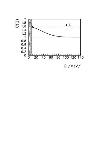
Figure 1:

Figure 2:

Figure 3:

Figure 4:

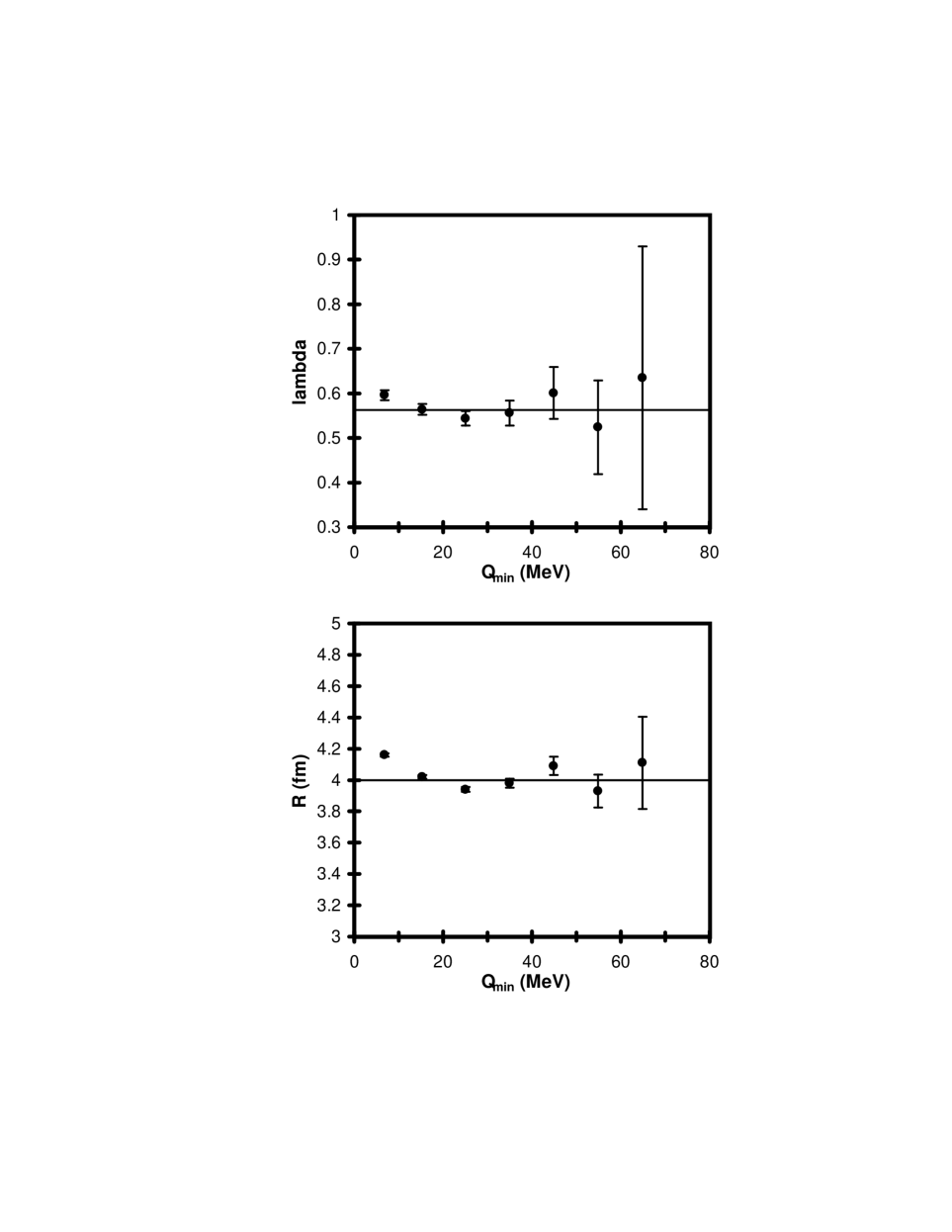
Figure 5:

Figure 6:

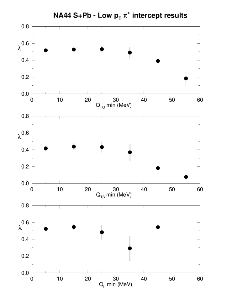
Figure 7:

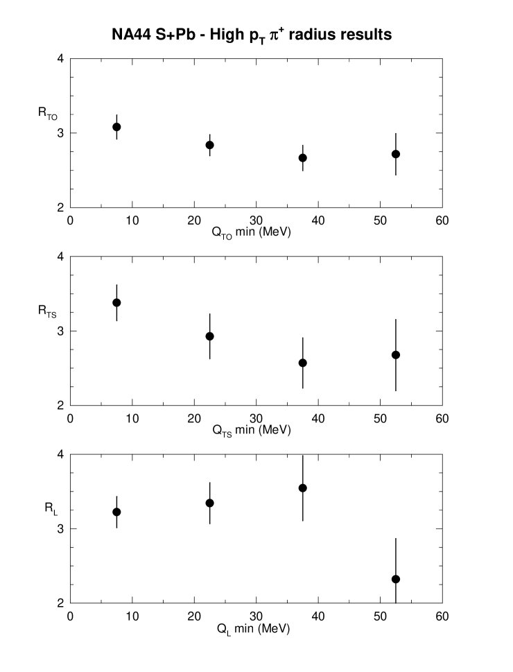
Figure 8:

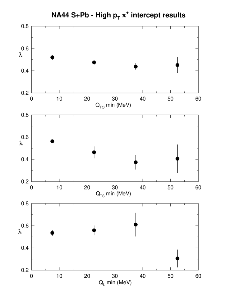
Figure 9:

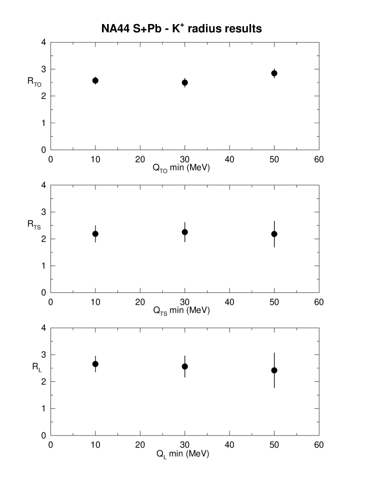
Figure 10:

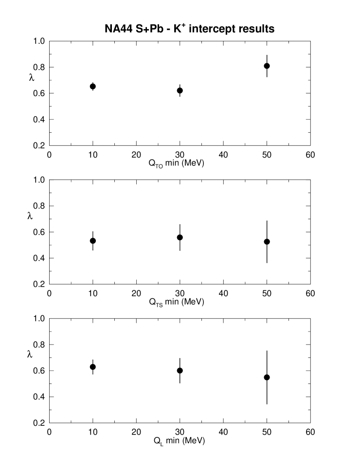
Figure 11:

Figure 12:

References

- [1] R. Hanbury-Brown and R.Q. Twiss, Nature 178, 1046 (1956).
- [2] G. Goldhaber, W. B. Fowler, S. Goldhaber, T. F. Hoang, T. E. Kalogeropolous and W. M. Powell, Phys. Rev. Lett 3 (1959) 181.
- [3] G. Goldhaber, S. Goldhaber, W. Lee, and A. Pais, Phys. Rev. 120, 300 (1960).
- [4] M. Gyulassy, S. K. Kaufmann and L. W. Wilson, Phys. Rev. C20, (1979) 2267
- [5] H. Beker et al, Phys. Rev. Lett. 74, 3340 (1995).
- [6] T. Csörgő, B. Lörstad, and J. Zimányi, hep-ph/9411307, Z. Phys. C 71 (1996) 491
- [7] T. Csörgő, hep-ph/9705422, Phys. Lett. B 409 (1997) 11
- [8] S. Pratt, T. Csörgő and J. Zimányi, Phys. Rev. C42 (1990) 2646
- [9] William Zajc, in Particle Production in Highly Excited Matter, ed. by H. Gutbord and J. Rafelski, NATO ASI series B303 (Plenum Press, New York, 1993) p. 435.
- [10] J. Zimányi and T. Csörgő, hep-ph/9705432 (Phys. Rev. Lett. (1997) in preparation).
- [11] S. Chapman, P. Scotto and U. Heinz, Heavy Ion Physics 1 (1995) 1
-
[12]
I. Andreev, M. Plümer, R. Weiner,
Int. J. Mod. Phys. A8(1993)4577;
M. Biyajima et al, Progr. Theor. Phys. 84(1990)931;
N. Suzuki, M. Biyajima, Progr. Theor. Phys. 88 (1992) 609. - [13] A. Bialas, Acta Physica Polonica B23 (1992) 561
- [14] G. F. Bertsch, Nucl. Phys. A498 (1989) 173c
- [15] T. Csörgő and S. Pratt, Report No. KFKI-1991-28/A p. 75
- [16] T. Csörgő and B. Lörstad, Phys. Rev. C 54 (1996) 1390
-
[17]
J. P. Sullivan et al, Phys. Rev. Lett. 70 (1993) 3000;
R. D. Fields et al, Phys. Rev. C52 (1995) 986 - [18] J. Bolz, U. Ornik, M. Plümer, B.R. Schlei, and R.M. Weiner, Phys. Lett. B 300, 404 (1993).
- [19] J. Bolz, U. Ornik, M. Plümer, B.R. Schlei, and R.M. Weiner, Phys. Rev. D 47, 3860 (1993).
- [20] H. Heiselberg, hep-ph/9602431, Phys. Lett. B. 379 (1996) 27
- [21] B. R. Schlei et al, Phys. Lett. B376 (1996) 212
- [22] U. Heinz, nucl-th/9609029, in Correlations and Clustering Phenomena in Subatomic Physics, Dronten, The Netherlands, Aug 4-18 1996 (NATO ASI Proc. Series, Plenum Press, to appear).
- [23] U. Heinz and U. A. Wiedemann, nucl-th/9611031
- [24] Yu. M. Sinyukov, S. V. Akkelin and Yu. A. Tolstkyh, Nucl. Phys. 610 (1996) 278c
- [25] S. Nickerson, “A Halo Model of Heavy Ion Collisions”, M. Sc. Thesis, Dalhousie University, Halifax, Canada, June 1996
- [26] T. Csörgő, S. Nickerson and D. Kiang, hep-ph/9611275
- [27] S. S. Padula and M. Gyulassy, Phys. Lett. B 348 (1995) 303
-
[28]
T. Akesson et al, AFS Collaboration,
Phys. Lett. B 129 (1983) 269 ;
Phys. Lett. B 187 (1987) 420 ; Z. Phys. C 36 (1987) 517. - [29] H. Beker et al, NA44 Collaboration, Z. Phys. C 64 (1994) 209
- [30] H. Bøggild et al, NA44 Collaboration, Phys. Lett. B 302 (1993) 510.
- [31] H. Bøggild et al, Phys. Lett. B 349, 386 (1995).
- [32] B. Lörstad (private communication).
- [33] W.H. Press, B.P. Flannery, S.A. Teukolsky, and W.T. Vetterling, Numerical Recipes : The Art of Scientific Computing, (Cambridge University Press, New York, 1987).
- [34] M. Sarabura, Nucl. Phys. A 544, 125c (1992).
- [35] J. Dodd, NA44 Collaboration, Proc. XXV-th ISMPD, Stara Lesna, Slovakia, Sept. 1995. (D. Bruncko et al., eds, World Scientific, Singapore, 1996)
- [36] S. Chapman, P. Scotto, and U. Heinz, Phys. Rev. Lett. 74, 4400 (1995).
- [37] H. Beker et al, Z. Phys. C 64, 209 (1994).
- [38] T. Alber for the NA35/NA49 Collaborations, Nucl. Phys. A 590 (1995) 453c.
- [39] T. Csörgő, talk at the HBT’96 conference, ECT*, Trento, Italy, September 1996.
- [40] D. Miskowiecz, talk at the HBT’96 conference, ECT*, Trento, Italy, September 1996.
- [41] S. E. Vance, T. Csörgő and D. Kharzeev, in preparation.