Proton Polarization in the $p(\vec{e},e^{\prime}\vec{p})\pi^{0}$
Reaction and the Measurement
of Quadrupole Components
in the N to $\Delta$ Transition

Abstract

The recoil proton polarization in the $\pi^{0}$ production off the proton with longitudinally polarized electron beam has been studied as a means to measure quadrupole components in the N to $\Delta$ transition. On top of the $\Delta$ resonance a high sensitivity to a possible Coulomb quadrupole excitation is found in parallel kinematics. The ratio of $S_{1+}/M_{1+}$ multipole amplitudes can be determined from the ratio of the two in-scattering-plane recoil proton polarization components. Avoiding the absolute measurement of the polarizations, such a ratio allows small experimental uncertainties. Furthermore, the electron helicity independent proton polarization component enables the characterization of resonant and non-resonant pieces.

PACS: 14.20.Gk; 13.60.Rj; 13.60.Le; 13.40.-f; 13.60.-r

1 Introduction and Motivation

The occurrence of quadrupole components in the N to $\Delta$ transition is within quark models related to d-state configurations in the nucleon and/or the $\Delta$ wavefunction [1, 2]. They originate from details of the inner dynamics of the composite nucleon like a color hyperfine interaction in the one-gluon-exchange [3] and, therefore, are of interest for the understanding of the nucleon structure. The precise measurement of the quadrupole amplitudes is a long standing experimental problem due to their smallness compared to the dominating magnetic dipole amplitude. Only observables carrying interference terms between the large and the small amplitudes offer sufficient sensitivity for a reliable determination. Appropriate interferences are accessible in $\Delta^{+}$-electroproduction experiments off the proton where the resonance is tagged by its decay into proton and $\pi^{0}$, and either the pion or the recoiling proton is detected in coincidence with the scattered electron. Early coincidence experiments at NINA [4] and DESY [5, 6, 7] extracted, with large experimental uncertainties, ratios of Coulomb quadrupole to magnetic dipole strength, $S_{1+}/M_{1+}$, around $-6\%$ over a range of four-momentum transfers of $0.3$ to $1.56$ (GeV/c)². A fixed-t dispersion-relation based reanalysis [8] of older data [9, 10, 11] yielded surprisingly large numbers of about $-15\%$ at momentum transfers down to $0.047$ (GeV/c)². A comparatively large ratio of $(-11.0\pm 3.7)\%$ was also obtained in a recent experiment at ELSA, which measured the azimuthal angular distribution of the high energetic photon from the $\pi^{0}$-decay around the momentum transfer direction [12]. All the experiments extracted the sum of resonant and non-resonant quadrupole components. A separation was achieved for the first time in a pion-photoproduction experiment at MAMI. There, a linearly polarized tagged photon beam was used to determine photon asymmetries simultaneously for both neutral and charged pion production [13], thus enabling the decomposition into isospin $1/2$ and $3/2$ channels of the electric quadrupole amplitude, E2, at the photon point.

Further insight into the electric quadrupole admixture of the N to $\Delta$ transition could be obtained by a precise determination of the resonant $S_{1+}/M_{1+}$ ratio as a function of four-momentum transfer. This would constrain the spatial distribution of the electric charge in the transition.

Polarized electron beams in combination with polarized proton targets or recoil proton polarimetry open possibilities for new approaches. The $p(\vec{e},e^{\prime}\vec{p})\pi^{0}$ reaction has been examined with regard to a measurement of the longitudinal quadrupole component in the N to $\Delta$ transition and the separation of resonant and non-resonant pieces. The next section recalls briefly the general formalism for $\pi^{0}$-electroproduction and then discusses the possibilities of recoil polarization measurements, particularly in parallel kinematics where the recoiling proton is detected in momentum transfer direction. Section 3 evaluates important experimental aspects and the main conclusions are summarized in section 4.

2 The $p(\vec{e},e^{\prime}\vec{p})\pi^{0}$ Reaction

Following the notation of Raskin and Donnelly [14], the differential cross section for the $p(\vec{e},e^{\prime}\vec{p})\pi^{0}$ reaction can be written as

$$\left(\frac{d\sigma}{dE^{\prime}\Omega_{e}\Omega_{p}^{cm}}\right) = \mbox{$K_{Mott}$}\cdot\{(v_{L}R_{fi}^{L}+v_{T}R_{fi}^{T}+v_{TT}R_{fi}^{TT}+v_{LT}R_{fi}^{LT})+$$ (1)

$$\qquad\qquad+h(v_{T^{\prime}}R_{fi}^{T^{\prime}}+v_{LT^{\prime}}R_{fi}^{LT^{\prime}})\}$$

with

$$K_{Mott}=\frac{M_{p}m_{\pi}p_{p}^{cm}}{8\pi^{3}W}\sigma_{Mott}\,\mbox{.}$$ (2)

$W$ is the invariant mass of the recoiling hadronic system, $p_{p}^{cm}$ the proton momentum in the center-of-momentum frame, and $M_{p}$ and $m_{\pi}$ are the proton and pion rest mass, respectively. The electron kinematics enters into the factors $v_{M}$ ($M=L,T,TT,LT,T^{\prime},LT^{\prime}$):

$$v_{L} = \left(\frac{Q^{2}}{\vec{q}\,^{2}}\right)^{2}\cdot\left(\frac{W}{M_{p}}\right)^{2}$$

$$v_{T} = \frac{1}{2}\left(\frac{Q^{2}}{\vec{q}\,^{2}}\right)+\tan^{2}\frac{\vartheta_{e}}{2}$$

$$v_{TT} = -\frac{1}{2}\left(\frac{Q^{2}}{\vec{q}\,^{2}}\right)$$

$$v_{LT} = -\frac{1}{\sqrt{2}}\left(\frac{Q^{2}}{\vec{q}\,^{2}}\right)\sqrt{\left(\frac{Q^{2}}{\vec{q}\,^{2}}\right)+\tan^{2}{\frac{\vartheta_{e}}{2}}}\cdot\frac{W}{M_{p}}$$

$$v_{T^{\prime}} = \sqrt{\left(\frac{Q^{2}}{\vec{q}\,^{2}}\right)+\tan^{2}{\frac{\vartheta_{e}}{2}}}\tan{\frac{\vartheta_{e}}{2}}$$

$$v_{LT^{\prime}} = -\frac{1}{\sqrt{2}}\left(\frac{Q^{2}}{\vec{q}\,^{2}}\right)\tan{\frac{\vartheta_{e}}{2}}\cdot\frac{W}{M_{p}}$$ (3)

In the above equations, $\vartheta_{e}$ is the electron scattering angle, $\vec{q}\,^{2}$ the square of the three-momentum transfer, $Q^{2}=4EE^{\prime}\sin^{2}(\vartheta_{e}/2)$ is the negative squared four-momentum transfer, and $h$ is the longitudinal polarization of the electron beam. The structure of the hadronic system is contained in the six structure functions $R_{fi}^{M}$, which implicitly contain the proton polarization. The dependence on proton polarization can be made explicit, leading to a total of 18 structure functions [14, 15] in the cross section:

$$\left(\frac{d\sigma}{dE^{\prime}\Omega_{e}\Omega_{p}^{cm}}\right) = K_{Mott}\cdot\Big{\{}v_{L}(\mbox{$R_{L}$}+\Pi_{n}\mbox{$R_{L}^{n}$})+v_{T}(\mbox{$R_{T}$}+\Pi_{n}\mbox{$R_{T}^{n}$})+$$ (4)

$$\quad v_{LT}\left[(\mbox{$R_{LT}$}+\Pi_{n}\mbox{$R_{LT}^{n}$})\cos\Phi+(\Pi_{l}l\mbox{$R_{LT}^{l}$}+\Pi_{t}\mbox{$R_{LT}^{t}$})\sin\Phi\right]+$$

$$\quad v_{TT}\left[(\mbox{$R_{TT}$}+\Pi_{n}\mbox{$R_{TT}^{n}$})\cos{2\Phi}+(\Pi_{l}\mbox{$R_{TT}^{l}$}+\Pi_{t}\mbox{$R_{TT}^{t}$})\sin{2\Phi}\right]+$$

$$\quad h\cdot\Big{\{}v_{LT^{\prime}}\left[(\mbox{$R_{LT^{\prime}}$}+\Pi_{n}\mbox{$R_{LT^{\prime}}^{n}$})\sin\Phi+(\Pi_{l}\mbox{$R_{LT^{\prime}}^{l}$}+\Pi_{t}\mbox{$R_{LT^{\prime}}^{t}$})\cos\Phi\right]+$$

$$\qquad v_{T^{\prime}}\left[\Pi_{l}\mbox{$R_{TT^{\prime}}^{l}$}+\Pi_{t}\mbox{$R_{TT^{\prime}}^{t}$}\right]\Big{\}}\Big{\}}$$

$\Pi_{n,l,t}=\pm 1$ are the projections of the proton spin in its rest frame onto the axes $n$, $l$, $t$ depicted in Fig.1. The longitudinal unit vector, $\hat{l}$, is in the direction of the proton momentum in the center-of-momentum frame, $\hat{n}=\hat{q}\times\hat{l}/\sin{\mbox{$\theta_{p}^{cm}$}}$ points normal to the reaction plane and $\hat{t}=\hat{n}\times\hat{l}$ is perpendicular to the proton momentum in the reaction plane. The connection between the R structure functions and the W structure functions as defined by Raskin and Donnelly [14] is given in the appendix.

Figure 1: Reference frames for the recoil proton polarization

From the cross section of Eq.(4) one gets for the recoil proton polarization components

$$\sigma_{0}P_{l} = \mbox{$K_{Mott}$}\left\{v_{LT}\mbox{$R_{LT}^{l}$}\sin\Phi+v_{TT}\mbox{$R_{TT}^{l}$}\sin 2\Phi+h\left[v_{LT^{\prime}}\mbox{$R_{LT^{\prime}}^{l}$}\cos\Phi+v_{T^{\prime}}\mbox{$R_{TT^{\prime}}^{l}$}\right]\right\}$$

$$\sigma_{0}P_{t} = \mbox{$K_{Mott}$}\left\{v_{LT}\mbox{$R_{LT}^{t}$}\sin\Phi+v_{TT}\mbox{$R_{TT}^{t}$}\sin 2\Phi+h\left[v_{LT^{\prime}}\mbox{$R_{LT^{\prime}}^{t}$}\cos\Phi+v_{T^{\prime}}\mbox{$R_{TT^{\prime}}^{t}$}\right]\right\}$$ (5)

$$\sigma_{0}P_{n} = \mbox{$K_{Mott}$}\left\{v_{L}\mbox{$R_{L}^{n}$}+v_{T}\mbox{$R_{T}^{n}$}+v_{LT}\mbox{$R_{LT}^{n}$}\cos\Phi+v_{TT}\mbox{$R_{TT}^{n}$}\cos 2\Phi+hv_{LT^{\prime}}\mbox{$R_{LT^{\prime}}^{n}$}\sin\Phi\right\},$$

where $\sigma_{0}$ represents the proton polarization independent part of the cross section. The recoil proton polarization can be split into the electron polarization dependent part (transferred polarization), $P_{\{n,l,t\}}^{\prime}$, which is proportional to $h$, and an electron polarization independent induced polarization. From the above equations the transferred polarization components are given by:

$$\sigma_{0}P_{t}^{\prime} = h\cdot\mbox{$K_{Mott}$}\cdot\left[v_{T^{\prime}}\mbox{$R_{TT^{\prime}}^{t}$}+v_{LT^{\prime}}\mbox{$R_{LT^{\prime}}^{t}$}\cos{\Phi}\right]$$

$$\sigma_{0}P_{l}^{\prime} = h\cdot\mbox{$K_{Mott}$}\cdot\left[v_{T^{\prime}}\mbox{$R_{TT^{\prime}}^{l}$}+v_{LT^{\prime}}\mbox{$R_{LT^{\prime}}^{l}$}\cos{\Phi}\right]$$ (6)

$$\sigma_{0}P_{n}^{\prime} = h\cdot\mbox{$K_{Mott}$}\cdot v_{LT^{\prime}}\mbox{$R_{LT^{\prime}}^{n}$}\sin{\Phi}$$

There are two terms contributing to the polarization component $P_{t}^{\prime}$. The first one is independent of $\Phi$ and points always into $t$ direction of the reaction plane reference frame, which rotates with the out-of-plane angle $\Phi$ (see Fig.1). Viewed from the electron scattering plane, the polarization related to this term points into opposite directions left ($\Phi=0$) and right ($\Phi=\pi$) of $\vec{q}$ and therefore vanishes in the case of parallel kinematics $\mbox{$\theta_{p}^{cm}$}=0$. Correspondingly, $R_{TT^{\prime}}^{t}$  carries an implicit $\sin\mbox{$\theta_{p}^{cm}$}$-dependence. The second term depends on $\cos\Phi$, like the projection of a polarization which is fixed in the electron scattering plane onto the rotating $\{n,l,t\}$ frame. This part does not vanish in parallel kinematics.

Similarly the other components of Eq.(2) also contain projections of a fixed polarization in the electron scattering plane. The natural choice for a polarization, $P$, that is fixed in the electron scattering plane is the $\{x,y,z\}$ frame of Fig.1, which is related to the $\{n,l,t\}$ system by a simple rotation:

$$P_{x} = \mbox{$P_{l}$}\sin\mbox{$\theta_{p}^{cm}$}\cos\Phi+\mbox{$P_{t}$}\cos\mbox{$\theta_{p}^{cm}$}\cos\Phi-\mbox{$P_{n}$}\sin\Phi$$

$$P_{y} = \mbox{$P_{l}$}\sin\mbox{$\theta_{p}^{cm}$}\sin\Phi+\mbox{$P_{t}$}\cos\mbox{$\theta_{p}^{cm}$}\sin\Phi+\mbox{$P_{n}$}\cos\Phi$$ (7)

$$P_{z} = \mbox{$P_{l}$}\cos\mbox{$\theta_{p}^{cm}$}-\mbox{$P_{t}$}\sin\mbox{$\theta_{p}^{cm}$}$$

In the case of parallel kinematics this transformation remains still defined. The angle $\Phi$ then plays the role of the orientation of the transverse polarization, $P_{t}$, relative to the electron scattering plane.

The proton polarization components can be expressed by the multipole decomposition of the structure functions according to [14]. Restricting the expansion in the usual way to s and p waves and retaining only terms with the dominant $M_{1+}$ amplitude, one gets for the case of strictly parallel kinematics with $\mbox{$\theta_{p}^{cm}$}=0$:

$$\sigma_{0}P_{x} = h\cdot\mbox{$K_{LT^{\prime}}$}\cdot\sqrt{2}\cdot\Re\left\{S_{0+}^{*}M_{1+}+S_{1-}^{*}M_{1+}+4S_{1+}^{*}M_{1+}\right\}$$ (8)

$$\sigma_{0}P_{y} = -\mbox{$K_{LT}$}\cdot\sqrt{2}\cdot\Im\left\{S_{0+}^{*}M_{1+}+S_{1-}^{*}M_{1+}+4S_{1+}^{*}M_{1+}\right\}$$ (9)

$$\sigma_{0}P_{z} = h\cdot\mbox{$K_{T^{\prime}}$}\cdot\left[|M_{1+}|^{2}+\Re\left\{6E_{1+}M_{1+}^{*}+2M_{1+}(E_{0+}^{*}-M_{1-}^{*})\right\}\right]$$ (10)

with

$$K_{M}=K_{Mott}\cdot v_{M}\cdot\frac{4\pi W^{2}}{\alpha m_{\pi}M_{p}^{2}}~{};~{}~{}~{}M=LT^{\prime},LT,T^{\prime}\mbox{.}$$ (11)

The two in-plane components, $P_{x}$ and $P_{z}$, are proportional to the electron helicity, $h$, and vanish with unpolarized electron beam. Contrary, the component normal to the electron scattering plane, $P_{y}$, is independent of $h$ and thus shows up already with unpolarized beam.

$P_{x}$ carries in parallel kinematics a high sensitivity to the small longitudinal quadrupole amplitude, $S_{1+}$, due to the interference with the large $M_{1+}$ amplitude. It is, however, not solely determined by resonant amplitudes, but receives both resonant and non-resonant contributions. The induced polarization, $P_{y}$ (Eq.9), measures the imaginary part of the same combinations of interference terms of which $P_{x}$ (Eq.8) determines the real part. This offers the possibility to disentangle resonant and non-resonant pieces, which will later be discussed in more detail. $P_{z}$ is dominated by $|M_{1+}|^{2}$. Therefore, the ratio of the two in-plane polarization components, $P_{x}/P_{z}$, is directly related to $S_{1+}/M_{1+}$. $P_{x}$ and $P_{z}$ are simultaneously accessible behind a (spin precessing) magnetic system like a proton spectrometer. In the ratio $P_{x}/P_{z}$ the absolute values of both the electron beam polarization and the analyzing power of the proton polarimeter cancel out, which otherwise represent major sources of systematic uncertainties.

With real detectors the polarization components are averaged over finite acceptances around parallel kinematics. This will be discussed in the next section along with the influence of the non-leading terms in the s and p wave approximation.

2.1 Polarization observables in the laboratory frame

The considerations of the preceeding section illustrate the sensitivity of the recoil proton polarization to the $S_{1+}$ quadrupole amplitude for parallel kinematics. A real experiment will cover a finite solid angle around the strictly parallel case. Therefore, in this section the azimuthal averaging of the polarization components $P_{x,y,z}^{lab}$ is considered. For this discussion the polarization (Eq.(2)) is projected from the center-of-momentum into the laboratory frame [16]. The corresponding transformation is given by the so-called Wigner-rotation [17]:

$$P_{t}^{lab} = P_{t}\cos{\vartheta_{W}}+P_{l}\sin{\vartheta_{W}}$$

$$P_{l}^{lab} = -P_{t}\sin{\vartheta_{W}}+P_{l}\cos{\vartheta_{W}}$$ (12)

$$P_{n}^{lab} = P_{n}$$

The Wigner angle, $\vartheta_{W}$, is given by

$$\sin{\vartheta_{W}}=\frac{1+\gamma}{\gamma^{cm}+\gamma^{lab}}\cdot\sin(\mbox{$\theta_{p}^{cm}$}-\theta_{p}^{lab}),$$ (13)

where the Lorentz factors $\gamma$, $\gamma^{cm}$ and $\gamma^{lab}$ are related to the velocities of the center-of-momentum frame against the laboratory frame, and of the proton in the cm and lab frames, respectively. The transformation

$$P_{x}^{lab} = \mbox{$P_{l}$}^{lab}\sin\theta_{p}^{lab}\cos\Phi+\mbox{$P_{t}$}^{lab}\cos\theta_{p}^{lab}\cos\Phi-\mbox{$P_{n}$}^{lab}\sin\Phi$$

$$P_{y}^{lab} = \mbox{$P_{l}$}^{lab}\sin\theta_{p}^{lab}\sin\Phi+\mbox{$P_{t}$}^{lab}\cos\theta_{p}^{lab}\sin\Phi+\mbox{$P_{n}$}^{lab}\cos\Phi$$ (14)

$$P_{z}^{lab} = \mbox{$P_{l}$}^{lab}\cos\theta_{p}^{lab}-\mbox{$P_{t}$}^{lab}\sin\theta_{p}^{lab}$$

projects the polarization as seen in the laboratory reaction plane (Eq.(2.1)) onto the {x,y,z}-frame related to the electron scattering plane. The {x,y,z}-components of Eq.(2.1) are azimuthally averaged around the direction of the momentum transfer, $\vec{q}$, which is indicated by the bar in the following equations. Only those terms with even powers of $\sin\Phi$ and $\cos\Phi$ survive the integration over $\Phi$. Keeping for the sake of clarity only terms containing the dominant $M_{1+}$ amplitude, the result is:

$$(\overline{\sigma_{0}P_{x}})^{lab} = h\cdot\mbox{$K_{LT^{\prime}}$}\cdot\sqrt{2}\cdot\Re\big{\{}S_{0+}^{*}M_{1+}\cdot\frac{1}{2}\big{[}-4\sin\mbox{$\theta_{p}^{cm}$}(\sin\mbox{$\theta_{p}^{lab}$}\cos\mbox{$\vartheta_{W}$}+\cos\mbox{$\theta_{p}^{lab}$}\sin\mbox{$\vartheta_{W}$})$$ (15)

$$\qquad+\cos\mbox{$\theta_{p}^{cm}$}(\cos\mbox{$\theta_{p}^{lab}$}\cos\mbox{$\vartheta_{W}$}-\sin\mbox{$\theta_{p}^{lab}$}\sin\mbox{$\vartheta_{W}$}+1)\big{]}\quad+$$

$$S_{1-}^{*}M_{1+}\cdot\frac{1}{2}\big{[}1+(2-\cos^{2}\mbox{$\theta_{p}^{cm}$})(\cos\mbox{$\theta_{p}^{lab}$}\cos\mbox{$\vartheta_{W}$}-\sin\mbox{$\theta_{p}^{lab}$}\sin\mbox{$\vartheta_{W}$})$$

$$\qquad-\sin\mbox{$\theta_{p}^{cm}$}\cos\mbox{$\theta_{p}^{cm}$}(\cos\mbox{$\theta_{p}^{lab}$}\sin\mbox{$\vartheta_{W}$}+\sin\mbox{$\theta_{p}^{lab}$}\cos\mbox{$\vartheta_{W}$})\big{]}\quad+$$

$$S_{1+}^{*}M_{1+}\cdot\frac{1}{2}\big{[}4(2\cos^{2}\mbox{$\theta_{p}^{cm}$}-1)(\cos\mbox{$\theta_{p}^{lab}$}\cos\mbox{$\vartheta_{W}$}-\sin\mbox{$\theta_{p}^{lab}$}\sin\mbox{$\vartheta_{W}$})$$

$$\qquad-10\cos\mbox{$\theta_{p}^{cm}$}\sin\mbox{$\theta_{p}^{cm}$}(\cos\mbox{$\theta_{p}^{lab}$}\sin\mbox{$\vartheta_{W}$}+\sin\mbox{$\theta_{p}^{lab}$}\cos\mbox{$\vartheta_{W}$})$$

$$\qquad+2(3\cos^{2}\mbox{$\theta_{p}^{cm}$}-1)\big{]}\big{\}}$$

$$(\overline{\sigma_{0}P_{y}})^{lab} = -\mbox{$K_{LT}$}\cdot\sqrt{2}\cdot\Im\big{\{}S_{0+}^{*}M_{1+}\cdot\frac{1}{2}\big{[}-4\sin\mbox{$\theta_{p}^{cm}$}(\sin\mbox{$\theta_{p}^{lab}$}\cos\mbox{$\vartheta_{W}$}+\cos\mbox{$\theta_{p}^{lab}$}\sin\mbox{$\vartheta_{W}$})$$ (16)

$$\qquad+\cos\mbox{$\theta_{p}^{cm}$}(\cos\mbox{$\theta_{p}^{lab}$}\cos\mbox{$\vartheta_{W}$}-\sin\mbox{$\theta_{p}^{lab}$}\sin\mbox{$\vartheta_{W}$}+1)\big{]}\quad+$$

$$S_{1-}^{*}M_{1+}\cdot\frac{1}{2}\big{[}1+(2-\cos^{2}\mbox{$\theta_{p}^{cm}$})(\cos\mbox{$\theta_{p}^{lab}$}\cos\mbox{$\vartheta_{W}$}-\sin\mbox{$\theta_{p}^{lab}$}\sin\mbox{$\vartheta_{W}$})$$

$$\qquad-\sin\mbox{$\theta_{p}^{cm}$}\cos\mbox{$\theta_{p}^{cm}$}(\cos\mbox{$\theta_{p}^{lab}$}\sin\mbox{$\vartheta_{W}$}+\sin\mbox{$\theta_{p}^{lab}$}\cos\mbox{$\vartheta_{W}$})\big{]}\quad+$$

$$S_{1+}^{*}M_{1+}\cdot\frac{1}{2}\big{[}4(2\cos^{2}\mbox{$\theta_{p}^{cm}$}-1)(\cos\mbox{$\theta_{p}^{lab}$}\cos\mbox{$\vartheta_{W}$}-\sin\mbox{$\theta_{p}^{lab}$}\sin\mbox{$\vartheta_{W}$})$$

$$\qquad-10\cos\mbox{$\theta_{p}^{cm}$}\sin\mbox{$\theta_{p}^{cm}$}(\cos\mbox{$\theta_{p}^{lab}$}\sin\mbox{$\vartheta_{W}$}+\sin\mbox{$\theta_{p}^{lab}$}\cos\mbox{$\vartheta_{W}$})$$

$$\qquad+2(3\cos^{2}\mbox{$\theta_{p}^{cm}$}-1)\big{]}\big{\}}$$

$$(\overline{\sigma_{0}P_{z}})^{lab} = h\cdot\mbox{$K_{T^{\prime}}$}\cdot\big{\{}|M_{1+}|^{2}\big{[}(2-\cos^{2}\mbox{$\theta_{p}^{cm}$})(\cos\mbox{$\theta_{p}^{lab}$}\cos\mbox{$\vartheta_{W}$}-\sin\mbox{$\theta_{p}^{lab}$}\sin\mbox{$\vartheta_{W}$})$$ (17)

$$\qquad-\sin\mbox{$\theta_{p}^{cm}$}\cos\mbox{$\theta_{p}^{cm}$}(\cos\mbox{$\theta_{p}^{lab}$}\sin\mbox{$\vartheta_{W}$}+\sin\mbox{$\theta_{p}^{lab}$}\cos\mbox{$\vartheta_{W}$})\big{]}\quad+$$

$$\Re\{6M_{1+}^{*}E_{1+}\}\big{[}(2\cos^{2}\mbox{$\theta_{p}^{cm}$}-1)(\cos\mbox{$\theta_{p}^{lab}$}\cos\mbox{$\vartheta_{W}$}-\sin\mbox{$\theta_{p}^{lab}$}\sin\mbox{$\vartheta_{W}$})$$

$$\qquad-\sin\mbox{$\theta_{p}^{cm}$}\cos\mbox{$\theta_{p}^{cm}$}(\cos\mbox{$\theta_{p}^{lab}$}\sin\mbox{$\vartheta_{W}$}+\sin\mbox{$\theta_{p}^{lab}$}\cos\mbox{$\vartheta_{W}$})\big{]}\quad+$$

$$\Re\{M_{1-}^{*}M_{1+}\}\big{[}(-1-\cos^{2}\mbox{$\theta_{p}^{cm}$})(\cos\mbox{$\theta_{p}^{lab}$}\cos\mbox{$\vartheta_{W}$}-\sin\mbox{$\theta_{p}^{lab}$}\sin\mbox{$\vartheta_{W}$})$$

$$\qquad-\sin\mbox{$\theta_{p}^{cm}$}\cos\mbox{$\theta_{p}^{cm}$}(\cos\mbox{$\theta_{p}^{lab}$}\sin\mbox{$\vartheta_{W}$}+\sin\mbox{$\theta_{p}^{lab}$}\cos\mbox{$\vartheta_{W}$})\big{]}\quad+$$

$$\Re\{E_{0+}^{*}M_{1+}\}\big{[}2\cos\mbox{$\theta_{p}^{cm}$}(cos\mbox{$\theta_{p}^{lab}$}\cos\mbox{$\vartheta_{W}$}-\sin\mbox{$\theta_{p}^{lab}$}\sin\mbox{$\vartheta_{W}$})$$

$$\qquad-\sin\mbox{$\theta_{p}^{cm}$}(\cos\mbox{$\theta_{p}^{lab}$}\sin\mbox{$\vartheta_{W}$}+\sin\mbox{$\theta_{p}^{lab}$}\cos\mbox{$\vartheta_{W}$})\big{]}\big{\}}$$

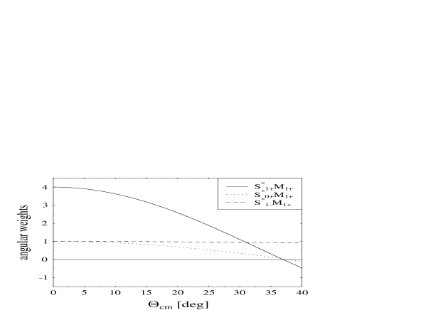
Figure 2: Relative angular weights of the leading multipole terms of $P_{x}$ and $P_{y}$, which are the same for both components (see text), for the kinematics described in section 3.1.

The angular coefficients of the interference terms are the same in Eq.(15) and (16). They are plotted in Fig.2. The sensitivity to the $S_{1+}^{*}M_{1+}$ interference term decreases with increasing $\theta_{p}^{cm}$. $S_{0+}^{*}M_{1+}$ shows practically the same behaviour, but reduced by a factor 4, while the weight of $S_{1-}^{*}M_{1+}$ is almost constant.

In the limit of parallel kinematics, Eqs.(15-17) reduce to Eqs.(8-10). Keeping also the non-leading terms in the s and p wave approximation, one arrives at:

$$(\overline{\sigma_{0}P_{x}})^{lab}_{\theta\rightarrow 0} = \mbox{$K_{LT^{\prime}}$}\cdot h\cdot\sqrt{2}\cdot\Re\big{\{}(S_{0+}^{*}+S_{1-}^{*}+4S_{1+}^{*})(E_{0+}+3E_{1+}+M_{1+}-M_{1-})\big{\}}~{}~{}~{}$$ (18)

$$(\overline{\sigma_{0}P_{y}})^{lab}_{\theta\rightarrow 0} = -\mbox{$K_{LT}$}\cdot\sqrt{2}\cdot\Im\big{\{}(S_{0+}^{*}+S_{1-}^{*}+4S_{1+}^{*})(E_{0+}+3E_{1+}+M_{1+}-M_{1-})\big{\}}~{}~{}~{}$$ (19)

$$(\overline{\sigma_{0}P_{z}})^{lab}_{\theta\rightarrow 0} = \mbox{$K_{T^{\prime}}$}\cdot h\cdot\Big{[}|E_{0+}|^{2}+9|E_{1+}|^{2}+|M_{1-}|^{2}+|M_{1+}|^{2}$$ (20)

$$\quad+\Re\left\{2E_{0+}^{*}(6E_{1+}+M_{1+}-M_{1-})+6M_{1+}^{*}E_{1+}-2M_{1-}^{*}M_{1+}\right\}\Big{]}.$$

Thus, in parallel kinematics, $P_{y}$ contains the imaginary part of the same interference terms as the real part in $P_{x}$. This fact can be exploited for a separation of contributions due to the Delta-resonance from other contributions, which are caused either by non-resonant $\pi^{0}$-production or by higher nucleon resonances.

2.2 Separation of resonant and non-resonant pieces

The multipole amplitudes of Eqs.(18-20) are not solely determined by the $\Delta$-resonance, but contain both resonant and non-resonant pieces. Therefore, in the following, the multipole combinations of $P_{x}$ and $P_{y}$ (Eqs.18 and 19) are split into their resonant and non-resonant parts. This is closely related to the decomposition of the physical $\pi^{0}$-electroproduction amplitudes, $A_{i}^{\pi^{0}}$, into isospin $\frac{1}{2}$ and $\frac{3}{2}$ channels [18].

$$A_{i}^{\pi^{0}}=A_{i}^{1/2}+\frac{2}{3}A_{i}^{3/2}\hskip 8.5359pt;\hskip 28.45274ptA=M,\,E,\,S$$ (21)

As stated by the Watson Final State Theorem [19], all $A_{1+}^{3/2}$ amplitudes show the almost purely resonant behaviour of $M_{1+}^{3/2}$. All other multipoles are considered as non-resonant.

$$S_{0+}^{*}+S_{1-}^{*}+4S_{1+}^{*} = [S_{0+}^{1/2}+S_{1-}^{1/2}+4S_{1+}^{1/2}+\frac{2}{3}(S_{0+}^{3/2}+S_{1-}^{3/2})]^{*}+\frac{8}{3}(S_{1+}^{3/2})^{*}$$ (22)

$$= [S_{non}^{*}]+S_{res}^{*}$$

$$E_{0+}+3E_{1+}+M_{1+}-M_{1-} = [E_{0+}^{1/2}+3E_{1+}^{1/2}+M_{1+}^{1/2}-M_{1-}^{1/2}+\frac{2}{3}(E_{0+}^{3/2}-M_{1-}^{3/2})]$$ (23)

$$\quad+\frac{2}{3}(3E_{1+}^{3/2}+M_{1+}^{3/2})$$

$$= [E,M_{non}]+E,M_{res}\mbox{.}$$

If, at the position of the $\Delta$ resonance, all terms without the by far dominating $\Im\{M_{1+}^{3/2}\}$ are neglected, Eqs.(18) and (19) can be written as

$$(\overline{\sigma_{0}P_{x}})^{lab}_{\theta\rightarrow 0} = \mbox{$K_{LT^{\prime}}$}\cdot h\cdot\sqrt{2}\cdot\Im\{S_{non}^{*}+S_{res}^{*}\}\cdot\frac{2}{3}\Im\{M_{1+}^{3/2}\}$$ (24)

$$(\overline{\sigma_{0}P_{y}})^{lab}_{\theta\rightarrow 0} = -\mbox{$K_{LT}$}\cdot\sqrt{2}\cdot\Re\{S_{non}^{*}\}\cdot\frac{2}{3}\Im\{M_{1+}^{3/2}\}$$ (25)

The real parts of resonant amplitudes vanish directly on top of the resonance and therefore the corresponding terms do not occur in the above equations. According to Eqs.(24) and (25) $P_{x}$ measures the sum of the resonant longitudinal quadrupole component, $S_{res}^{*}=\frac{8}{3}(S_{1+}^{3/2})^{*}$, and nonresonant contributions, $S_{non}^{*}$, whereas $P_{y}$ is solely sensitive to $S_{non}^{*}$. In the (hypothetical) case of a single, pure resonance where all real parts vanish on top of the resonance, $P_{y}$ would thus be identical zero.

However, purely real Born terms $S_{0+}^{1/2,3/2}$, $S_{1-}^{1/2,3/2}$, and $S_{1+}^{1/2}$ result already in a nonvanishing $P_{y}$. On the other hand, for real Born terms $\Im\{S_{non}\}$ vanishes, i.e. Eq.(24) yields:

$$(\overline{\sigma_{0}P_{x}})^{lab}_{\theta\rightarrow 0}=\mbox{$K_{LT^{\prime}}$}\cdot h\cdot\sqrt{2}\cdot\frac{16}{9}\cdot\Im\{(S_{1+}^{3/2})^{*}\}\cdot\Im\{M_{1+}^{3/2}\}$$ (26)

This means that, within the approximations discussed, $P_{x}$ contains directly the wanted isospin 3/2 part of the $S_{1+}$ amplitude.

Non-Born contributions might occur due to either rescattering processes or higher resonances, like $S_{1-}^{1/2}$ from the Roper N(1440). If there were non-Born imaginary parts contributing, Eq.(26) would be more complicated. Such terms are in principle detectable through $P_{y}$, because real and imaginary parts of the amplitudes are related by fixed phases as requested by Watson’s Final State Theorem. Therefore imaginary parts in $S_{non}$ go along with an altered real part $\Re\{S_{non}\}$ as compared to purely real non-resonant amplitudes.

3 Experimental aspects

The polarization of recoil protons can be measured in a focal plane polarimeter behind a magnetic spectrometer, like the proton polarimeter [20] of the A1 collaboration [21] at MAMI. Such a device measures the azimuthal asymmetry of protons which were inclusively scattered in a carbon secondary scatterer. With this process, only the two polarization components perpendicular to the proton momentum are accessible. Due to the spin precession in the spectrometer magnetic system, these two polarization components measured in the focal plane are linear combinations of all three components at the target, $P_{x},P_{y},P_{z}$. Provided a complete understanding of the spin precession, the measurement of only two focal plane polarization components is nevertheless sufficient to determine all three target components, because there is additional information from flipping the electron beam helicity: $P_{x}$ and $P_{z}$ are odd under helicity reversal, while $P_{y}$ is even (cf. Eqs.(8-10)).

The averaging over the azimuthal angle, $\Phi$, which leads to the expressions discussed in section 2.1, can be easily accomplished in the case of parallel kinematics where the spectrometer sits in the momentum transfer direction. Here the sensitivity to the longitudinal quadrupole amplitude, $S_{1+}$, is maximum. It is higher than in previously proposed experiments with distinct measurements left and right of the momentum transfer direction [22, 23, 24]. The comparatively high degree of proton polarization in those experiments is only due to the mixing of the large $P_{z}$ component, which according to Eq.(17) contains a $|M_{1+}|^{2}$ term, into the considered $P_{t}$ polarization components at finite angles $\theta_{p}^{cm}$.

In contrast to a non-magnetic polarimeter, where the longitudinal proton polarization component is inaccessible, $P_{x}$ and $P_{z}$ can be measured simultaneously behind the spectrometer. This allows the mesaurement of the ratio $P_{x}/P_{z}$ with obvious advantages:

1. The leading term of this ratio is directly $\Re\{S_{1+}^{*}M_{1+}\}/|M_{1+}|^{2}$.

2. In the polarization ratio the absolute value of the electron beam polarization cancels out.

3. The recoil polarizations are determined by polarimeter asymmetries with a common effective analyzing power. The polarization ratio is thus also independent of the absolute value of the polarimeter’s analyzing power.

Therefore such a measurement can be performed without monitoring the electron beam polarization. The beam polarization need even not be constant over time, because both recoil polarization components are measured truely simultaneously. The absolute calibration of the effective polarimeter analyzing power is neither required, since in the ratio it cancels out, too. A similar polarization-ratio method was successfully employed in a recent measurement of the neutron electric formfactor [25, 26].

The influence of possible non-Born contributions to the measured ratio can be studied via the induced polarization, $P_{y}$. This component is independent of the electron beam polarization and thus more sensitive to false systematic asymmetries. For the analysis of $P_{y}$ the absolute calibration of the proton polarimeter is therefore desirable, although a ratio measurement $P_{y}/P_{z}$ could also be imagined. In any case, the beam polarization must be known, since in the $P_{y}/P_{z}$-ratio the polarimeter analyzing power cancels, but the beam polarization does not.

3.1 Expected proton polarizations in a realistic experiment

Accounting only for the leading terms in the above expressions (cf. Eqs.(8,10)) and neglecting a possible offset due to imaginary parts of the non-resonant amplitudes, the recoil proton polarization in parallel kinematics can be estimated by

$$P_{x} = \frac{1}{\sigma_{0}}h\mbox{$K_{Mott}$}v_{LT^{\prime}}N^{2}\sqrt{2}\Re\{4S_{1+}^{*}M_{1+}\}$$ (27)

$$P_{z} = \frac{1}{\sigma_{0}}h\mbox{$K_{Mott}$}v_{T^{\prime}}N^{2}|M_{1+}|^{2}\mbox{.}$$ (28)

With the proton polarization independent cross section approximated through

$$\sigma_{0}=\mbox{$K_{Mott}$}v_{T}N^{2}|M_{1+}|^{2}\mbox{,}$$ (29)

one receives

$$P_{x} = 4\sqrt{2}h\frac{v_{LT^{\prime}}}{v_{T}}\frac{\Re\{S_{1+}^{*}M_{1+}\}}{|M_{1+}|^{2}}$$ (30)

$$= -8h\frac{\tan(\vartheta_{e}/2)}{1+\frac{2\vec{q}\,^{2}}{Q^{2}}\tan^{2}(\vartheta_{e}/2)}\cdot\frac{W}{M_{p}}\cdot\frac{\Re\{S_{1+}^{*}M_{1+}\}}{|M_{1+}|^{2}}$$

$$= -8\cdot h\cdot\epsilon\cdot\tan(\vartheta_{e}/2)\cdot\frac{W}{M_{p}}\cdot\frac{\Re\{S_{1+}^{*}M_{1+}\}}{|M_{1+}|^{2}}\,,$$

$$P_{z} = h\frac{v_{T^{\prime}}}{v_{T}}\frac{|M_{1+}|^{2}}{|M_{1+}|^{2}}$$ (31)

$$= h\sqrt{1-\epsilon^{2}}\,.$$

$\epsilon=[1+(2\vec{q}\,^{2}/Q^{2})\tan^{2}\frac{\vartheta_{e}}{2}]^{-1}$ is the virtual photon’s degree of transverse polarization. Making use of the relations of appendix D of [15] between CGLN amplitudes [27] and structure functions, the above relation for $P_{z}$ can be shown to hold generally in parallel kinematics, i.e. independently of the approximations discussed. Fixed by kinematical variables only, $P_{z}$ might thus be used for calibration checks. Applying the electron kinematics of the MAMI $N$-$\Delta$ proposal [24], $E=0.855\,\mbox{GeV},\,W=1.232\,\mbox{GeV},\,Q^{2}=0.12\,\mbox{(GeV/c)}^{2},\,\vartheta_{e}=32^{o},\,|\vec{q}|=0.53\,\mbox{GeV}\,$, Eqs.(30) and (31) yield

$$P_{x} = -2.2\cdot h\cdot\frac{\Re\{S_{1+}^{*}M_{1+}\}}{|M_{1+}|^{2}}$$ (32)

$$P_{z} = 0.7\cdot h\,.$$ (33)

Thus, a quadrupole contribution of the order of $-5$ % causes a transverse proton polarization of $P_{x}\simeq 7.6\,\%$ with an electron beam polarization of 70 %, which now routinely is achieved [28]. The longitudinal proton polarization then is $P_{z}=49\,\%$.

4 Summary and conclusion

The $p(\vec{e},e^{\prime}\vec{p})\pi^{0}$ reaction with measurement of the recoil proton polarization has a large potential towards the precise determination of the longitudinal quadrupole component, $S_{1+}$, in the N to $\Delta$ transition. In particular in parallel kinematics, it offers on top of the $\Delta$ resonance a high sensitivity to the $S_{1+}^{*}M_{1+}$ interference term. This is clearly revealed when the process is discussed in the appropriate $\{x,y,z\}$ coordinate frame, which is fixed to the electron scattering plane (see Fig.1). Here the polarization transfer from the electron takes a simple form and is not obscured by projections onto rotating reference frames.

The ratio of the recoil proton polarization components, $P_{x}/P_{z}$, is directly related to $\Re\{S_{1+}^{*}M_{1+}\}/|M_{1+}|^{2}$. If both components are measured simultaneously after the deflection in a magnetic spectrometer, the absolute values of both electron beam polarization and polarimeter analyzing power cancel out. Therefore small experimental uncertainties can be achieved. The electron beam helicity independent polarization component, $P_{y}$, offers the opportunity to determine possible non-Born contributions.

5 Acknowledgements

I thank R. Beck, J. Friedrich, F. Klein and L. Tiator for many fruitful discussions. This work was supported by the Deutsche Forschungsgemeinschaft (SFB201).

Appendix

The relation between the R and W structure functions of [14] are explicitly:

$$\hat{R}_{L} =W^{L}(0) \qquad\hat{R}_{L}^{n} =W^{L}(n) \qquad\hat{R}_{T} =W^{T}(0) \qquad\hat{R}_{T}^{n} =W^{T}(n)$$

$$\hat{R}_{TT} =W^{TT}(0) \qquad\hat{R}_{TT}^{n} =W^{TT}(n) \qquad\hat{R}_{TT}^{l} =\tilde{W}^{TT}(l) \qquad\hat{R}_{TT}^{t} =\tilde{W}^{TT}(s)$$

$$\hat{R}_{LT} =W^{TL}(0) \qquad\hat{R}_{LT}^{n} =W^{TL}(n) \qquad\hat{R}_{LT}^{l} =\tilde{W}^{TL}(l) \qquad\hat{R}_{LT}^{t} =\tilde{W}^{TL}(s)$$

$$\hat{R}_{LT^{\prime}} =\tilde{W}^{TL^{\prime}}(0) \qquad\hat{R}_{LT^{\prime}}^{n} =\tilde{W}^{TL^{\prime}}(n) \qquad\hat{R}_{LT^{\prime}}^{l} =W^{TL^{\prime}}(l) \qquad\hat{R}_{LT^{\prime}}^{t} =W^{TL^{\prime}}(s)$$

$$\qquad\hat{R}_{TT^{\prime}}^{l} =W^{T^{\prime}}(l) \qquad\hat{R}_{TT^{\prime}}^{t} =W^{T^{\prime}}(s)$$

with

$$\hat{R}_{M}=\frac{R_{M}}{N^{2}}\qquad\mbox{and}\qquad N^{2}=\frac{4\pi W^{2}}{\alpha m_{\pi}M_{N}^{2}}.$$

References

• [1] S.S. Gershtein et al., Sov. J. Nucl. Phys. 34, 870 (1981)
• [2] N. Isgur et al., Phys. Rev. D 25, 2394 (1982)
• [3] S.L. Glashow, Physica A 96, 27 (1979)
• [4] R. Siddle et al., Nucl. Phys. B 35, 93 (1971)
• [5] J.C. Alder et al., Nucl. Phys. B 46, 573 (1972)
• [6] W. Albrecht et al., Nucl. Phys. B 25, 1 (1971)
• [7] W. Albrecht et al., Nucl. Phys. B 27, 615 (1971)
• [8] R.L. Crawford et al., Nucl. Phys. B 28, 573 (1971)
• [9] C.W. Akerlof et al., Phys. Rev. 163, 1482 (1967)
• [10] C. Mistretta et al., Phys. Rev. 184, 1487 (1969)
• [11] K. Baba et al., Nuovo Cimento 59A, 53 (1969)
• [12] F. Kalleicher et al., Z. Phys. A 359, 201 (1997)
• [13] R. Beck et al., Phys. Rev. Lett. 78, 606 (1997) and
H.P. Krahn, doctoral thesis, Mainz 1996
• [14] A.S. Raskin and T.W. Donnelly, Ann. of Phys. 191, 78 (1989)
• [15] D. Drechsel and L. Tiator, J. Phys. G: Nucl. Part. Phys. 18, 449 (1992)
• [16] V. Dmitrasinovic and F. Gross, Phys. Rev. C 40, 2479 (1989)
• [17] D.R. Giebink, Phys. Rev. C 32, 502 (1985) and references therein
• [18] see for example:
A.A. Komar (ed.), β€œPhotoproduction of Pions on Nucleons and Nuclei”, Proceedings of the Lebedev Physics Institute Academy of Science of the USSR, Volume 186, Nova Science Publishers, New York and Budapest 1989
• [19] K.M. Watson, Phys. Rev. 95, 228 (1954)
• [20] T. Pospischil, doctoral thesis, Mainz (in preparation)
• [21] K.I. Blomqvist et al., accepted for publication in Nucl. Instr. Methods A
• [22] R. Lourie, Nucl. Phys. A 509, 653 (1990)
• [23] Proposal #89-03 β€œPolarization Observables in Pion Electroproduction at the $\Delta$(1232) Resonance”, MIT-Bates, Cambridge, MA, USA (1989)
• [24] Proposal A1/3-93 β€œMeasurement of $E2/C2$ contributions in the $N\rightarrow\Delta$ transition through the $p(\vec{e},e^{\prime}\vec{p})\pi^{0}$ reaction”, MAMI, University of Mainz, Germany (1993)
• [25] F. Klein, Proceedings of the 14th International Conference on Particles and Nuclei, PANIC’96, Williamsburg, VA, USA (1996), p.121
• [26] M. Ostrick, doctoral thesis, Mainz (in preparation)
• [27] G.F. Chew et al., Phys. Rev. 106, 1345 (1957)
• [28] K. Aulenbacher et al., Nucl. Instrum. Methods A 391, 498 (1997)