Two photons decay of the glueball and scalar isoscalar mesons in a scaled NJL model

Abstract

We use a modified version of the Nambu–Jona-Lasinio model which implements the QCD trace anomaly to calculate the two photons decay width of the glueball ($f_{0}(1500)$) and of the two scalar mesons ($f_{0}(1370)$, $f_{J=0}(1710)$) to which it is mixed. We investigate the effect of this mixing over the coupling constants of the $f_{0}$ states to the quarks.

,

1 Introduction

The scalar resonance $f_{0}(1500)$ which has been discovered at LEAR by the Crystal Barrel Collaboration in the reaction $p\overline{p}$ (at rest) $\rightarrow 3{\pi}^{0},\eta\eta{\pi}^{0}$ [1] and $\eta\eta\ ^{\prime}{\pi}^{0}$ [2], was immediately considered as a good candidate for the scalar glueball. Indeed, the observed mass ((1520$\pm$25) MeV in [1] and (1545$\pm$25) MeV in [2]) was near the value predicted by the lattice-QCD calculations [3] of that time. It is also in agreement with the analysis of recent data on the decay $f_{0}(1500)\rightarrow K\overline{K}$ [4] which however requires a mixture between the glueball and the neighbouring $q\overline{q}$ states [5]. Another signal that strengthens this identification lies in the fact that, in the radiative decay $J/\psi\rightarrow\gamma+4\pi$, a sharp peak is seen in the 4$\pi$ spectrum, having quantum numbers ${0}^{++}$ and mass and width also compatible with $f_{0}(1500)$ [6].

The mixing between the glueball and the $q\overline{q}$ states has also been noted by Sexton et al. [7]. They however identify the nearly glueball state with $f_{J}(1710)$ whose mixing with $f_{0}(1370)$ and $f_{0}(1500)$ requires that $J=0$ [5], [8].

In Refs. [8], [9], it has been claimed that good tests of the glue and $q\overline{q}$ contents of the glueball would consist in studying its partial strong decay widths into $\pi\pi,K\overline{K},\eta\eta^{\prime},\eta\eta$. We plan to calculate them in a forthcoming paper [10].

In the present paper, we follow the idea of Close et al. [5] who estimate the two photons decay widths of the glueball and of the mesons to which it is mixed. Emission of photons is surely a good test to investigate the glueball or $q\overline{q}$-nature of the $f_{0}$ states since gluons do not couple to photons. The authors suggest a mixing between $f_{0}(1370)$, $f_{0}(1500)$ and $f_{0}(1710)$ for which they study two different schemes, according to the preceding remarks. Firstly, they consider the case where $f_{0}(1500)$ exhibits large contents in glue and in $q\overline{q}$ ($u$ and $s$) excitations while $f_{0}(1710)$ has its largest component in the $s\overline{s}$ chanel. This allows to reproduce the $f_{0}(1500)\rightarrow K\overline{K}$ data [4]. The second scheme consists in considering the glueball lying above the $s\overline{s}$ member of the nonet [7]: $f_{0}(1710)$ can then be the glueball while $f_{0}(1500)$ is mainly a $s\overline{s}$ excitation. Within these two schemes, Close et al. [5] have estimated the relative strength of the $2\gamma$ widths for the three $f_{0}$ states:

$$f_{0}(1370):f_{0}(1500):f_{0}(1710)\approx 12:1:3,\hskip 28.45274pt(\mbox{scheme 1})$$

$$f_{0}(1370):f_{0}(1500):f_{0}(1710)\approx 13:0.2:3.\hskip 19.91692pt(\mbox{scheme 2})$$

Whatever the mixing, the decay width of $f_{0}(1500)$ is always the smallest. Experimental estimation of the $2\gamma$ widths would then be a good test of the general idea of $q\overline{q}$ and glue mixing. Indeed, if the width of the $f_{0}(1500)$ was found to be larger than one of the others, the idea of mixing would be destroyed. Note that the decay $f_{0}(1370)\rightarrow 2\gamma$ is the only one that has been measured experimentally : $\Gamma_{f_{0}(1370)}=5.4\pm 2.3$ KeV [11].

The model we use to calculate the two photons decay widths is a modified version of the SU(3) NJL model [12] which implements the trace anomaly of QCD [13]. It is called the scaled NJL model. It entails the introduction of a scalar field $\chi$ whose mean value $\chi_{0}$ can be identified with the vacuum gluon condensate [14]. This $\chi$ field couples to the quarks so that our model can describe the processes schematically shown in Fig. 1. In our model, it is the vacuum gluon condensate that fixes the mixing [15]: the smaller $\chi_{0}$, the larger the mixing.

Figure 1: Schematic $2\gamma$ decay of the glueball and of a scalar state.

However, in the domain of $\chi_{0}$ which allows to roughly reproduce the meson masses, $f_{0}(1710)$ remains mainly a $s\overline{s}$ excitation. Its coupling to the up quark is weak. In contrast, the strength of the coupling to the $u$ or $s$ quark is roughly of the same order of magnitude for $f_{0}(1370)$ and for $f_{0}(1500)$. In our model, the three states have glue content. $f_{0}(1500)$ is the one which yields to pure glueball if no mixing and it is the state that always has the largest glue content even if that of $f_{0}(1370)$ can become important. We then work in a scheme similar to the scheme 1 presented above.

The parameters of the model are fixed to reproduce the pion and kaon masses, the pion decay constant and the masses of $a_{0}(1450)$ $[{u\overline{d},\overline{u}d,{1\over\sqrt{2}}(u\overline{u}-d\overline{d})}]$ and $f_{0}(1500)$. The mass of the largest member of the nonet ($f_{0}(1710)$) will then vary as well as that of $f_{0}(1370)$. The latter is very sensitive to the value of the vacuum gluon condensate while the former keeps a value not far away from $1710$ MeV, whatever $\chi_{0}$ .

For completeness, let us add that the $2\gamma$ decay of the scalar mesons has also been studied in Ref. [16] within a relativistic quark model with linear confinement and instanton-induced interaction. $f_{0}(1500)$ and $f_{0}(980)$ are there considered as mixing between $u\overline{u}$ and $s\overline{s}$ states. Another relativistic treatment using a OGE model has been presented in Ref. [17].

Our paper is organized as follows. Section 2 recalls the useful tools of the scaled NJL model. Section 3 is devoted to the derivation of the decay widths of the mesons and of the glueball. We insist on the fact that the mixing between the three fields generating the glueball and the scalar mesons modifies the transition amplitudes. For instance, $f_{0}(1370)$ can decay into $2\gamma$ through the production of a $s\overline{s}$ pair. The estimation of the widths assumess the knowledge of the masses of the mesons and the glueball as well as their coupling constants to the quarks. These quantities are defined in Section 4. We discuss our results in Section 5. Finally, Section 6 gives our conclusions.

2 The model

The model used in this paper is described in Refs. [12, 18] under the name of ”A-scaling model”. We recall here some of the useful tools for the understanding of the present work. We start from the vacuum SU(3) effective Lagrangian:

$${\cal L}_{eff}(q,\bar{q},\chi) = \bar{q}(-i{\partial}_{\mu}\gamma_{\mu}+m)q$$ (1)

$$\mbox{}+\frac{1}{2a^{2}\chi^{2}}\sum_{i=0}^{8}[(\bar{q}\frac{(\lambda^{i})_{F}}{2}q)^{2}+(\bar{q}i\gamma_{5}\frac{((\lambda^{i})_{F}}{2}q)^{2}]+{\cal L}_{\chi}$$

which yields to the bosonized effective Euclidean action

$$I_{eff}(\varphi,\chi) = -{\rm Tr}_{\Lambda\chi}\ln(-i{\partial}_{\mu}\gamma_{\mu}+m+\Gamma_{a}\varphi_{a})$$ (2)

$$\hskip 85.35826pt\mbox{}+\int{d}^{4}x\frac{a^{2}\chi^{2}}{2}\varphi_{a}\varphi_{a}+\int{d}^{4}x{\cal L}_{\chi}$$

once one has integrated out the quark degrees of freedom. The meson fields write:

$$\varphi_{a}=(\sigma_{a},\pi_{a}),\hskip 42.67912pt\Gamma_{a}=(\lambda_{a},i\gamma_{5}\lambda_{a}),\hskip 42.67912pta=0,...,8$$ (3)

where the $\lambda_{a}$ are the usual Gell-Mann matrices with $\lambda_{0}={\sqrt{2/3}\bf{1}}$. We choose to work in the isospin symmetry limit and the quantity $\it m$ stands for the diagonal matrix ${\mathrm{diag}}(m_{u},m_{u},m_{s})$. The trace anomaly of QCD is modelized using a scalar dilaton field $\chi$ that is intimately related to the gluon condensate $\chi\propto{\langle G^{2}_{\mu\nu}\rangle}^{1/2}$ [12]:

$${\cal L_{\chi}}=\frac{1}{2}(\partial_{\mu}\chi)^{2}+\frac{1}{16}b^{2}(\chi^{4}\ln\frac{\chi^{4}}{\chi^{4}_{G}}-(\chi^{4}-\chi^{4}_{G})).$$ (4)

Since we are only interested in the scalar sector, the axial anomaly which would give the $\eta$-$\eta$’ mass difference is not considered here. Our model contains six parameters: the current quark masses ($m_{u},m_{s}$), the strengths ($a^{2},b^{2}$), the gluon parameter $\chi_{G}$ and the cut-off $\Lambda$ introduced to regularize the diverging quark loop. Four of these parameters are adjusted to reproduce the pion mass ($m_{\pi}$), the weak pion decay constant ($f_{\pi}$), the kaon mass ($m_{K}$) and that of $f_{0}$(1500). We then have two free parameters that we choose to be the vacuum gluon condensate $\chi_{0}$ (related to $\chi_{G}$ [18]) and the constituent up quark mass $M_{u}$. The latter is connected to the strength $a^{2}$ using the usual gap equation [12] which minimizes the action. Note that the strange constituent quark mass $M_{s}$ and $\chi_{0}$ obey similar stationary conditions. $M_{u}$ will have a large value ($725$ MeV) in order to reproduce $a_{0}(1450)$ [8] and $\chi_{0}$ will remain free.

3 The decay widths

The widths for the two photons decay of the scalar isoscalar mesons are given by

$$\Gamma_{i} = {1\over 2}{1\over 2{m}_{i}}{1\over(2\pi{)}^{2}}\int\int{{d}^{3}{k}_{1}\over 2\left|{{\vec{k}}_{1}}\right|}{{d}^{3}{k}_{2}\over 2\left|{{\vec{k}}_{2}}\right|}{\left|{{\cal T}_{i}}\right|}^{2}\delta(Q-{k}_{1}-{k}_{2})$$ (5)

$$= {1\over 32\pi}{1\over{m}_{i}}{\left|{{\cal T}_{i}}\right|}^{2}$$

for $i=f_{0}(1370),f_{0}(1710)$ and $f_{0}(1500)$. In Eq. (5), $m_{i}$ represents the mass of the meson, $Q$ its quadrimomentum while $k_{1}$ and $k_{2}$ stand for the quadrimomenta of the emerging photons. The mesons are assumed to be at rest. In a pure NLJ, the transition amplitude for $f_{0}(1500)$, identified with the glueball, is identically zero; ${\Gamma}_{{f}_{0}(1370)}$ only involves the propagator of the up quark (in the limit of isospin symmetry) while ${\Gamma}_{{f}_{0}(1710)}$ is expressed in terms of the strange quark propagator.

Figure 2: Feynman direct diagrams for $2\gamma$ decay of $f_{0}(1370)$ (a) and of $f_{0}(1710)$ (b).

The direct diagram (Fig. 2.a) writes

$${\cal T}_{{f}_{0}(1370)}={N}_{c}({e}_{u}^{2}+{e}_{d}^{2})\ {g}_{{f}_{0}(1370)}^{u\overline{u}}\ {\varepsilon}_{\mu}^{*}({k}_{1}){\varepsilon}_{\nu}^{*}({k}_{2})U$$ (6)

with

$$U = \int{d^{4}q_{3}\over(2\pi{)}^{4}}{\mathrm{tr}}_{D}\left\{{({q\!\!\!/}_{2}+{M}_{u}){\gamma}_{\mu}({q\!\!\!/}_{3}+{M}_{u}){\gamma}_{\nu}({q\!\!\!/}_{1}+{M}_{u})}\right\}$$ (7)

$$\times {1\over({q}_{1}^{2}+{M}_{u}^{2})({q}_{2}^{2}+{M}_{u}^{2})({q}_{3}^{2}+{M}_{u}^{2})}$$

while the direct diagram (Fig. 2.b) has the similar form:

$${\cal T}_{{f}_{0}(1710)}={N}_{c}{e}_{s}^{2}{g}_{{f}_{0}(1710)}^{s\overline{s}}{\varepsilon}_{\mu}^{*}({k}_{1}){\varepsilon}_{\nu}^{*}({k}_{2})S$$ (8)

with

$$S = \int{d^{4}q_{3}\over(2\pi{)}^{t4}}{\mathrm{tr}}_{D}\left\{{({q\!\!\!/}_{2}+{M}_{s}){\gamma}_{\mu}({q\!\!\!/}_{3}+{M}_{s}){\gamma}_{\nu}({q\!\!\!/}_{1}+{M}_{s})}\right\}$$ (9)

$$\times {1\over({q}_{1}^{2}+{M}_{s}^{2})({q}_{2}^{2}+{M}_{s}^{2})({q}_{3}^{2}+{M}_{s}^{2})}.$$

In the scaled NLJ, the mesons $f_{0}(1370)$ and $f_{0}(1710)$ are not anymore pure $u\overline{u}$ or pure $s\overline{s}$ excitations. Equations (6) and (8) have then to be modified in order to take these new effects into account:

$${\cal T}_{{f}_{0}(1370)} = {N}_{c}({e}_{u}^{2}+{e}_{d}^{2}){g}_{{f}_{0}(1370)}^{*u\overline{u}}{\varepsilon}_{\mu}^{*}({k}_{1}){\varepsilon}_{\nu}^{*}({k}_{2})U$$ (10)

$$\hskip 56.9055pt\mbox{}+{N}_{c}{e}_{s}^{2}{g}_{{f}_{0}(1370)}^{*s\overline{s}}{\varepsilon}_{\mu}^{*}({k}_{1}){\varepsilon}_{\nu}^{*}({k}_{2})S$$

$${\cal T}_{{f}_{0}(1710)} = {N}_{c}{e}_{s}^{2}{g}_{{f}_{0}(1710)}^{*s\overline{s}}{\varepsilon}_{\mu}^{*}({k}_{1}){\varepsilon}_{\nu}^{*}({k}_{2})S$$ (11)

$$\hskip 56.9055pt\mbox{}+{N}_{c}({e}_{u}^{2}+{e}_{d}^{2}){g}_{{f}_{0}(1710)}^{*u\overline{u}}{\varepsilon}_{\mu}^{*}({k}_{1}){\varepsilon}_{\nu}^{*}({k}_{2})U.$$

The quark meson coupling constants ${g}_{i}^{*u\overline{u}}$, ${g}_{i}^{*s\overline{s}}$, ($i=f_{0}(1370)$, $f_{0}(1710)$) differ from the ones introduced in Eqs. (6) and (8). Their analytical expressions will be established in Section. 4.

Having some content in $q\overline{q}$ excitations the glueball $f_{0}(1500)$ can now decay:

$${\cal T}_{{f}_{0}(1500)} = {N}_{c}({e}_{u}^{2}+{e}_{d}^{2}){g}_{{f}_{0}(1500)}^{*u\overline{u}\ }{\varepsilon}_{\mu}^{*}({k}_{1}){\varepsilon}_{\nu}^{*}({k}_{2})U$$ (12)

$$\hskip 56.9055pt\mbox{}+{N}_{c}{e}_{s}^{2}{g}_{{f}_{0}(1500)}^{*s\overline{s}}{\varepsilon}_{\mu}^{*}({k}_{1}){\varepsilon}_{\nu}^{*}({k}_{2})S.$$

Summing over the final polarization of the photon and using $Q=k_{1}+k_{2}$, $q_{1}=q-k_{2}$, $q_{2}=q+k_{1}$, $q_{3}=q$, one gets :

$${\left|{{\cal T}_{{f}_{0}(1370)}}\right|}^{2} = {12800\over 9}{\pi}^{2}{\alpha}^{2}\bigg{|}{({m}_{{f}_{0}(1370)}^{2}-4{M}_{u}^{2}){M}_{u}{g}_{{f}_{0}(1370)}^{*u\overline{u}}{J}_{u}(-{m}_{{f}_{0}(1370)}^{2})}\bigg{.}$$ (13)

$$+ {\bigg{.}{{1\over 5}({m}_{{f}_{0}(1370)}^{2}-4{M}_{s}^{2}){M}_{s}{g}_{{f}_{0}(1370)}^{*s\overline{s}}{J}_{s}(-{m}_{{f}_{0}(1370)}^{2})}\bigg{|}}^{2}$$

$${\left|{{\cal T}_{{f}_{0}(1710)}}\right|}^{2} = {12800\over 9}{\pi}^{2}{\alpha}^{2}\bigg{|}{({m}_{{f}_{0}(1710)}^{2}-4{M}_{u}^{2}){M}_{u}{g}_{{f}_{0}(1710)}^{*u\overline{u}}{J}_{u}(-{m}_{{f}_{0}(1710)}^{2})}\bigg{.}$$ (14)

$$+ {\bigg{.}{{1\over 5}({m}_{{f}_{0}(1710)}^{2}-4{M}_{s}^{2}){M}_{s}{g}_{{f}_{0}(1710)}^{*s\overline{s}}{J}_{s}(-{m}_{{f}_{0}(1710)}^{2})}\bigg{|}}^{2}$$

$${\left|{{\cal T}_{{f}_{0}(1500)}}\right|}^{2} = {12800\over 9}{\pi}^{2}{\alpha}^{2}\bigg{|}{({m}_{{f}_{0}(1500)}^{2}-4{M}_{u}^{2}){M}_{u}{g}_{{f}_{0}(1500)}^{*u\overline{u}}{J}_{u}(-{m}_{{f}_{0}(1500)}^{2})}\bigg{.}$$ (15)

$$+ {\bigg{.}{{1\over 5}({m}_{{f}_{0}(1500)}^{2}-4{M}_{s}^{2}){M}_{s}{g}_{{f}_{0}(1500)}^{*s\overline{s}}{J}_{s}(-{m}_{{f}_{0}(1500)}^{2})}\bigg{|}}^{2}$$

with

$${J}_{i}(Q)=\int{{d}^{4}q\over(2\pi{)}^{4}}{1\over\left[{(q+{k}_{1}{)}^{2}+{M}_{i}^{2}}\right]\left[{(q-{k}_{2}{)}^{2}+{M}_{i}^{2}}\right]\left[{{q}^{2}+{M}_{i}^{2}}\right]}$$ (16)

and $\alpha={e}^{2}/4\pi$ the fine structure constant. We will work with a large constituent up quark mass, $M_{u}$ = 725 MeV, in order to reproduce $a_{0}(1450)$. However, even with such a large mass, the mesons $f_{0}(1710)$ and the glueball (1500) always lie above the unphysical pair $u\overline{u}$ creation threshold $2M_{u}$. In the same way, $f_{0}(1710)$, which aquires a mass larger than $2M_{s}=1728$ MeV, is always above the $s\overline{s}$ threshold. The function $J_{u}$ should then be calculated in the complex plan:

$${J}_{u}\rightarrow{\left.{{J}_{u}({Q}^{2}-i{0}^{+})}\right|}_{{Q}^{2}=-({m}_{i}-{i{\Gamma}_{i}\over 2}{)}^{2}},$$ (17)

where $\Gamma_{i}$ is the width of the meson for its $u\overline{u}$ decay and with a similar expression for $J_{s}$. This width as well as the mass $m_{i}$ can be calculated from a Dyson-Schwinger equation (see below) which amounts to two coupled equations for $\Gamma_{i}$ and $m_{i}$. The latter cannot be decoupled without a suitable and model-dependent description. In the same way, expression (17) is here approximated by $\left|J_{u}(-{m_{i}}^{2}-i0^{+})\right|$. Note that the results are not significantly affected by the prescription used above the threshold. However, it would worth using a confining model to get rid of the unphysical decay channel. Indeed, Celenza et al. [19] have shown that a modification of the scalar vertex by a confining nonlocal interaction increases the mass of the ${\sigma}$ of $\approx 250$ MeV. This feature could surely modify quantitatively the results we present here.

4 Meson masses and coupling constants

Equations (13-15) involve the masses of the mesons as well as their coupling constants to the quarks $u$ and $s$. We now show how to calculate them, insisting on the way the coupling constants are modified due to the coupling between the various fields. The effective action (2) can be expanded up to second order in the fluctuating parts of the meson fields $({\tilde{\sigma}}_{0},{\tilde{\sigma}}_{8})$ and of the dilaton field $\tilde{\chi}$ :

$${I}^{(2)}({\sigma}_{0},{\sigma}_{8},\chi)={1\over 2\beta\Omega}\sum\limits_{q}({\tilde{\sigma}}_{0,q},{\tilde{\sigma}}_{8,q},{\tilde{\chi}}_{q}){S}^{-1}\left({\matrix{{\tilde{\sigma}}_{0,-q}\cr{\tilde{\sigma}}_{8,-q}\cr{\tilde{\chi}}_{-q}\cr}}\right).$$ (18)

$S^{-1}$ is a 3x3 matrix with 9 nonvanishing elements that can be read in Ref. [12]. It can be diagonalized, yielding to

$${I}^{(2)}({\phi}_{1},{\phi}_{2},{\phi}_{3})={1\over 2\beta\Omega}\sum\limits_{q}\sum\limits_{i}{\widetilde{\phi}}_{i,q}{\mathrm{diag}}\left[{{\Lambda}_{ii}({q}^{2})}\right]{\widetilde{\phi}}_{i,-q}.$$ (19)

with

$${\mathrm{diag}}\left[{{\Lambda}_{ii}({q}^{2})}\right]={V}^{T}(q^{2}){S}^{-1}V(q^{2}),$$ (20)

and $V$ the $q^{2}$ dependent eigenvector matrix. Expression (19) can be approximated by expanding the elements of the diagonal matrix around their respective zero, that is around the respective meson masses:

$${I}^{(2)}({\phi}_{1},{\phi}_{2},{\phi}_{3})\approx{1\over 2\beta\Omega}\sum\limits_{q}\sum\limits_{i}{\widetilde{\phi}}_{i,q}{\mathrm{diag}}\bigg{[}{{\Lambda}_{ii}}\bigg{.}(-{m}_{i}^{2})$$ (21)

$$\bigg{.}+({q}^{2}+{m}_{i}^{2}){\partial}_{{q}^{2}}{\Lambda}_{ii}{\bigg{.}{({q}^{2})}\bigg{|}}_{{q}^{2}=-{m}_{i}^{2}}\bigg{]}{\widetilde{\phi}}_{i,-q}$$ (22)

$$={1\over 2\beta\Omega}\sum\limits_{q}\sum\limits_{i}{\widetilde{\phi}}_{i,q}{G}_{i}^{-2}({q}^{2}+{m}_{i}^{2}){\widetilde{\phi}}_{i,-q}.$$ (23)

In Eq. (23), we have used the fact that

$${\mathrm{diag}}\left[{{\Lambda}_{ii}(-{m}_{i}^{2})}\right]=0$$ (24)

and we have defined [15]

$${G}_{i}^{-2}={\partial}_{{q}^{2}}{\mathrm{diag}}\left[{\Lambda}_{ii}(-{m}_{i}^{2})\right]={\left[{{V}^{T}(-{m}_{i}^{2})({\partial}_{{q}^{2}}{S}^{-1})V(-{m}_{i}^{2})}\right]}_{ii}$$ (25)

where the eigenvector matrix $V$ has its first row calculated at $-{m}_{1}^{2}=-{m}_{{f}_{0}(1370)}^{2}$, its second row at $-{m}_{2}^{2}=-{m}_{{f}_{0}(1710)}^{2}$ and the last one at $-{m}_{3}^{2}=-{m}_{{f}_{0}(1500)}^{2}$. The new physical fields ${\widetilde{\phi}}_{i}^{{}^{*}}$ associated with the three $f_{0}$ states write:

$${\widetilde{\phi}}_{i}^{{}^{*}}={G}_{i}^{-1}{\widetilde{\phi}}_{i}={G}_{i}^{-1}\sum\limits_{j}{V}_{ij}^{-1}(-{m}_{i}^{2}){\widetilde{\sigma}}_{j}$$ (26)

with ${\widetilde{\sigma}}_{1}\equiv{\widetilde{\sigma}}_{0},{\widetilde{\sigma}}_{2}\equiv{\widetilde{\sigma}}_{8},{\widetilde{\sigma}}_{3}\equiv\widetilde{\chi}$.

The interaction term in the quark loop ($\ln$) between the quarks and the meson fields (see Eq.(2)) reflects an interaction term in the Lagrangian of the form $\overline{q}({\sigma}_{0}{\lambda}_{0}+{\sigma}_{8}{\lambda}_{8})q$. Using Eq. (26), the latter becomes an interaction term between the quarks and the ${\widetilde{\phi}}_{i}^{{}^{*}}$:

$$\overline{q}({\sigma}_{0}{\lambda}_{0}+{\sigma}_{8}{\lambda}_{8})q=\overline{u}{A}_{1}u+\overline{d}{A}_{2}d+\overline{s}{A}_{3}{s}$$ (27)

with (there is no summation over the index i)

$${A}_{i}=\sum\limits_{j=1,2,3}{\widetilde{\phi}}_{j}^{{}^{*}}\left({({\lambda}_{0}{)}_{ii}{V}_{1j}+({\lambda}_{8}{)}_{ii}{V}_{2j}}\right){G}_{j}\ \ \ \ \ i=1,2,3$$ (28)

showing that the two mesons as well as the glueball are indeed coupled to the three quarks with the respective coupling constants:

$${g}_{j}^{*u\overline{u}}={g}_{j}^{*d\overline{d}} = \left[{({\lambda}_{0}{)}_{11}{V}_{1j}+({\lambda}_{8})_{11}{V}_{2j}}\right]{G}_{j}$$ (29)

$$g_{j}^{*s\overline{s}} = \left[{({\lambda}_{0}{)}_{33}{V}_{1j}+({\lambda}_{8}{)}_{33}{V}_{2j}}\right]{G}_{j},$$

$$\hskip 56.9055ptj=1({f}_{0}(1370)),2({f}_{0}(1710)),3({f}_{0}(1500)).$$

In a pure SU(3) NJL, without mixing with the dilaton, Eq. (28) reduces to

$${A}_{i}={\widetilde{\phi}}_{i}^{{}^{*}}{G}_{i}\ \ \ \ \ i=1,2$$ (31)

so that Eq. (25) defines the coupling constant of the mesons to the quark and ${\widetilde{\phi}}_{1}^{{}^{*}}\ ({\widetilde{\phi}}_{2}^{{}^{*}})$ is only coupled to the quark $u(s)$.

In the present approach, we will use Eqs. (24), (29), (4) to calculate the mass of the mesons and their respective coupling to the quarks. Note that it is the nonvanishing value of ${g}_{f_{0}(1500)}^{*u\overline{u}}$ and ${g}_{f_{0}(1500)}^{*s\overline{s}}$ that allows the glueball decay $f_{0}(1500)\rightarrow\gamma\gamma$.

As mentioned above, some caution must be taken when the $u\overline{u}$ or $s\overline{s}$ thresholds are reached. Due to the mixing with the glueball, it is not possible to solve analytically ${\mathrm{diag}}\left[{{\Lambda}_{ii}({q}^{2})}\right]$ (see Eq. (24)). In order to illustrate the threshold problem, we will drop here this mixing. The diagonalization then yields:

$${\Lambda}_{11}^{{}^{*}}({q}^{2})=4{N}_{c}{F}_{u}(q^{2})({q}^{2}+4{M}_{u}^{2})+{a}^{2}{\chi}_{0}^{2}{{m}_{u}\over{M}_{u}}$$ (32)

$${\Lambda}_{22}^{{}^{*}}({q}^{2})=4{N}_{c}{F}_{s}(q^{2})({q}^{2}+4{M}_{s}^{2})+{a}^{2}{\chi}_{0}^{2}{{m}_{s}\over{M}_{s}}$$ (33)

with

$${F}_{i}(q^{2})=\int{d}^{4}k{1\over\left[{(k-\frac{q}{2}{)}^{2}+{M}_{i}^{2}}\right]\left[{(k+{q\over 2}{)}^{2}+{M}_{i}^{2}}\right]}\ \ \ i=u,s.$$ (34)

Whenever the mesons lie below the threshold their mass is given by:

$${\Lambda}_{11}^{{}^{*}}(-{m}_{{f}_{0}(1370)}^{2})=0,\ \ {\Lambda}_{22}^{{}^{*}}(-{m}_{{f}_{0}(1710)}^{2})=0.$$ (35)

When the threshold is reached, Eq. (35) has to be modified to take into account the fact that the meson acquires a width due to its nonphysical decay into $u\overline{u}$ or $s\overline{s}$. This width and its mass are solutions of :

$${\Lambda}_{11}^{{}^{*}}{\left.{({q}^{2}-i\varepsilon)}\right|}_{{q}^{2}=-({m}_{{f}_{0}(1370)}-i{\Gamma}_{{f}_{0}(1370)}{)}^{2}}=0,$$ (36)

or more explicitly:

$$4{N}_{c}{F}_{u}\left[{-({m}_{{f}_{0}}+i\varepsilon-i{\Gamma}_{{f}_{0}}{)}^{2}}\right]\left[{-({m}_{{f}_{0}}-i{\Gamma}_{{f}_{0}}{)}^{2}+4{M}_{u}^{2}}\right]+{a}^{2}{\chi}_{0}^{2}{{m}_{u}\over{M}_{u}}=0,$$ (37)

with similar expression for ${f}_{0}(1710)$ with $u$ replaced by $s$. In order to get rid of the unphysical ${\Gamma}_{{f}_{0}}$, we perform here calculation with the approximated equations [15]

$$4{N}_{c}\left|{{F}_{i}\left[{-({m}_{{f}_{0}}+i\varepsilon{)}^{2}}\right]}\right|({-m}_{{f}_{0}}^{2}+4{M}_{u}^{2})+{a}^{2}{\chi}_{0}^{2}{{m}_{i}\over{M}_{i}}=0,\ \ i=u,s.$$ (38)

Other approximated expressions for the right-hand side of Eq. (37) can be found in the literature [20]. To our knowledge, Eq.(37) has never been solved exactly.

5 Results

The $\chi_{0}$ behavior for the mass of the three $f_{0}$ states is given in Fig. 3.

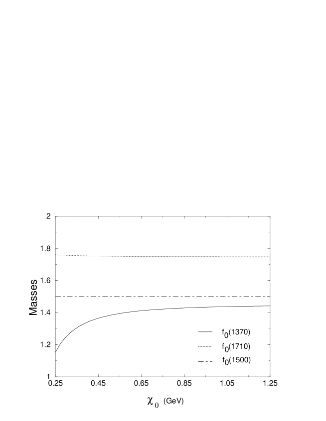
Figure 3: $\chi_{0}$ behavior of the mass of the three states $f_{0}(1370)$, $f_{0}(1500)$ and $f_{0}(1710)$.

For large values of $\chi_{0}$, the states take the mass they would have without coupling ($m_{f_{0}(1370)}=2M_{u}=1450$ MeV , $m_{f_{0}(1710)}=2M_{s}=1728$ MeV in the chiral limit). The mass of $f_{0}(1710)$ is quite stable while an acceptable value for the mass of $f_{0}(1370)$ limits the value of $\chi_{0}$ to a domain between 300 and 450 MeV (see Table 1).

Table 1: Masses and widths in $2\gamma$ of the hybrids $f_{0}(1370)$, $f_{0}(1710)$ and $f_{0}(1500)$.

		masses(MeV)	$\Gamma$(eV)	${\Gamma}/{\Gamma_{f_{0}(1710)}}$
	${f}_{0}(1370)$	1341	348	51.9
$\chi_{0}=400$ MeV	${f}_{0}(1500)$	1500	102	15.2
	${f}_{0}(1710)$	1753	6.7	1
	${f}_{0}(1370)$	1305	617	69.7
$\chi_{0}=350$ MeV	${f}_{0}(1500)$	1500	112	12.7
	${f}_{0}(1710)$	1755	8.85	1
	${f}_{0}(1370)$	1250	1258	102.3
$\chi_{0}=300$ MeV	${f}_{0}(1500)$	1500	123	10.0
	${f}_{0}(1710)$	1757	12.3	1

The same kind of behavior appears at the level of the coupling constants of the $f_{0}$ states to the quarks $u$ (Fig. 4, Eq. (29)) and $s$ (Fig. 5, Eq. (4)). Note that Fig. 4 and Fig. 5 exhibit the modulus of the coupling constants. Whenever the phase factor $(m_{f_{0}}^{2}-4M_{i}^{2})$ is negative, the corresponding coupling constant also becomes negative in such a way that the two contributions $u$ and $s$ add up (see Eqs. (13)–(15)). Here again, ${g}^{*u\overline{u}}$ and ${g}^{*s\overline{s}}$ are stable for the $f_{0}(1710)$ with ${g}^{*s\overline{s}}$ an order of magnitude larger than ${g}^{*u\overline{u}}$ indicating that $f_{0}(1710)$ is nearly a pure $s\overline{s}$ state. For large $\chi_{0}$, ${g}^{*u\overline{u}}_{f_{0}(1710)}{\rightarrow}0$. In contrast, the coupling constants ${g}^{*u\overline{u}}$ and ${g}^{*s\overline{s}}$ are of the same order of magnitude for $f_{0}(1370)$ and for $f_{0}(1500)$. At large $\chi_{0}$, ${g}_{{f}_{0}(1370)}^{*s\overline{s}}$ goes to zero, reflecting the fact ${f}_{0}(1370)$ is a pure $u\overline{u}$ state when the mixing is turned off. Finally, ${f}_{0}(1500){\rightarrow}2\gamma$ is forbidden in our model for large $\chi_{0}$, illustrated by the asymptotic behavior of ${g}_{{f}_{0}(1500)}^{*u\overline{u}}$ and ${g}_{{f}_{0}(1500)}^{*s\overline{s}}$ that vanish when $\chi_{0}{\rightarrow}\infty$. However, the decrease of the coupling constants of ${f}_{0}(1500)$ is slower than the others.

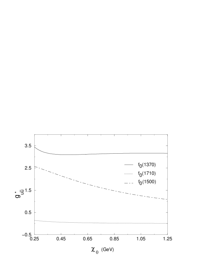
Figure 4: $\chi_{0}$ behavior of the coupling constant to the quark $u$, ${g}^{*u\overline{u}}$, of the three states $f_{0}(1370)$, $f_{0}(1500)$ and $f_{0}(1710)$.

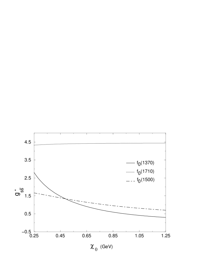
Figure 5: $\chi_{0}$ behavior of the coupling constant to the quark $s$, ${g}^{*s\overline{s}}$, of the three states $f_{0}(1370)$, $f_{0}(1500)$ and $f_{0}(1710)$.

The masses and the coupling constants so obtained allow to estimate the $2\gamma$ decay widths (Eqs. (5),(13)–(15)). Results are shown in Fig. 6. The three widths decrease with increasing $\chi_{0}$ since for $\chi_{0}\rightarrow\infty$, at least one of the corresponding coupling constants vanishes. $\Gamma_{f_{0}(1710)}$ is always the smallest because of two additionnal effects: in the RHS of Eq. (14) the first term is small due to the small value of ${g}_{{f}_{0}(1710)}^{*u\overline{u}}$ while the second one nearly vanishes due to the fact that $m_{f_{0}(1710)}\approx 2M_{s}$. For the two other states, the relative amplitude of the decays depends on the value of $\chi_{0}$.

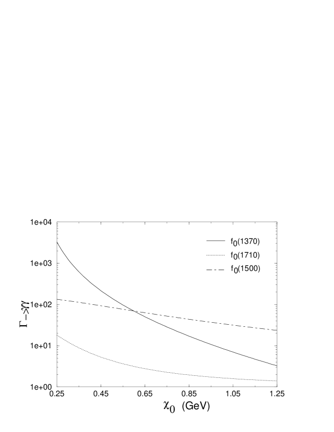
Figure 6: $\chi_{0}$ behavior of the width into $2\gamma$ of the three states $f_{0}(1370)$, $f_{0}(1500)$ and $f_{0}(1710)$.

For small $\chi_{0}$, $\Gamma_{f_{0}(1370)}>\Gamma_{f_{0}(1500)}$ due to four cumulative effects: $g_{f_{0}(1370)}^{*i\overline{i}}>g_{f_{0}(1500)}^{*i\overline{i}}$ and $\left|m_{f_{0}(1370)}^{2}-4M_{i}^{2}\right|>\left|m_{f_{0}(1500)}^{2}-4M_{i}^{2}\right|$ with $i=u,s$. For large $\chi_{0}$, $m_{f_{0}(1370)}\approx 2M_{u}$ and ${g}_{{f}_{0}(1370)}^{*s\overline{s}}$ becomes smaller while the RHS of Eq. (15) keeps two nonvanishing terms up to quite large values of $\chi_{0}$. One then has $\Gamma_{f_{0}(1370)}<\Gamma_{f_{0}(1500)}$. Note that in the chiral limit, the three widths go asymptotically to zero. (The factors $(m^{2}-4M^{2})$, which lead to a vanishing of the decay widths of $f_{0}(1370)$ and $f_{0}(1710)$ in the pure NJL model (no mixing) in the chiral limit, are a consequence of the chiral symmetry in the scalar sector. This was already shown by Bajc et al. Ref. [21].)

One then sees that our model provides meson and glueball widths that can vary from one to three orders of magnitude. Moreover, their relative magnitude is also $\chi_{0}$ dependent (see Fig. 7). Taking $\Gamma_{f_{0}(1710)}$ as reference, $\Gamma_{f_{0}(1370)}/\Gamma_{f_{0}(1710)}$ varies of two orders of magnitude and $\Gamma_{f_{0}(1500)}/\Gamma_{f_{0}(1710)}$, while more stable, can however vary of a factor 5 in the considered domain of $\chi_{0}$.

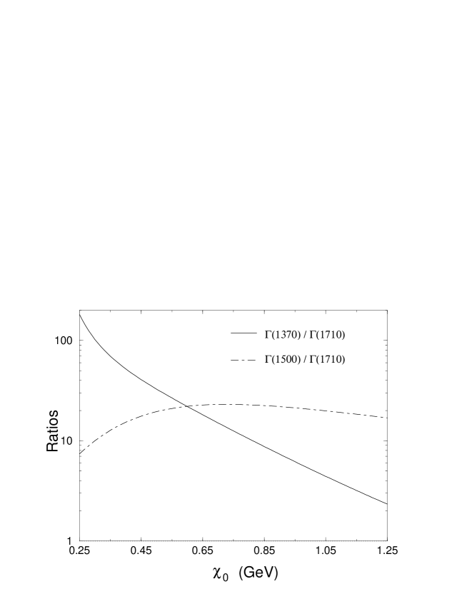
Figure 7: $\chi_{0}$ behavior of the ratios $\Gamma_{f_{0}(1370)}/\Gamma_{f_{0}(1710)}$ and $\Gamma_{f_{0}(1500)}/\Gamma_{f_{0}(1710)}$.

We have indicated in Table 1 the value of the widths as well as their ratio to $\Gamma_{f_{0}(1710)}$, for three typical values of $\chi_{0}$ compatible with the masses of the $f_{0}$ states.

Our results are in complete desagreement with the statement of Close et al. [5] presented in the introduction: the relative strengths are not reproduced, even qualitatively since the width $\Gamma_{f_{0}(1500)}$ is always larger than $\Gamma_{f_{0}(1710)}$. Moreover, the width of $f_{0}(1370)$ is always too small. To get the lower bound of the experimental value ($5.4\pm 2.3$ keV), one needs to consider gluon condensates as small as 270 MeV yielding a mass of $\approx 1200$ MeV and a still higher ratio $\Gamma$$/$$\Gamma_{f_{0}(1710)}$.

In order to compare our results with those of Ref. [16] it seems appropriate to compare our ratio $\Gamma_{f_{0}(1370)}$$/$$\Gamma_{f_{0}(1500)}$ with their result for $\Gamma_{f_{0}(980)}$$/$$\Gamma_{f_{0}(1590)}$. Indeed, in both cases the coupling of the two mesons to the $u\overline{u}$ and $s\overline{s}$ channels is important. Of course our model provides an additionnal glue content. One finds a quantity which varies from 3 to 10 while their corresponding result lies between 6 to 11.

6 Summary and conclusions

The model we developed in Refs. [14, 15] implements the QCD trace anomaly of QCD by the introduction of a dilaton scalar field $\chi$. (Other models of this type are on the market. See for example [22, 23] and references therein.) Since the NJL model is not renormalizable, a cut-off must be introduced to regularize the diverging integrals. This cut-off breaks the scale invariance of the quark loop that can be restored by the replacement $\Lambda\rightarrow\Lambda\chi$. This entails a mixing between the three scalar isoscalar fields. Put in an other way, one emerges with three scalar ”hybrids” $f_{0}$ which are mixing of glue and $u\overline{u}$ and $s\overline{s}$ excitations. We followed the idea of Close et al. [5] who identify these hybrids with $f_{0}(1370)$, $f_{0}(1500)$ and $f_{0}(1710)$. In our model, one has one free parameter, the vacuum gluon condensate $\chi_{0}$ that fixes the strength of the mixing. In the domain of $\chi_{0}$ (300 MeV $\leq\chi_{0}\leq 450$ MeV) which reproduces in an acceptable way the masses of the states, the mixing is quite large, reflected by the large values of the coupling constants to both types of quarks $u$ and $s$, especially for $f_{0}(1370)$ and $f_{0}(1500)$. The latter is identified with the glueball in the sense that it is the state that would yield pure glue if there was no mixing. In that case, it could not decay into $2\gamma$. Here this decay is allowed as well as that of the two other states. The relative magnitude of the widths largely depends on the value of the gluon condensate. However, whatever $\chi_{0}$, the width of $f_{0}(1710)$ is always the smallest. Our results are then at variance with that of Close et al. [5] according to which it is the width of $f_{0}(1500)$ that is always the smallest. They also claimed, that the idea of mixing should be revised if it was found experimentally that $\Gamma_{f_{0}(1500)}$ could exceed the width of the other states. We have however presented a model which yields totally different results while still including mixing and have shown that the reduction factors $(m^{2}-4M^{2})$ (playing almost no role for the $f_{0}(1500)$) are the key to understand the discrepancy between our results and those of [5]. Of course, our model contains some drawbacks, the most important being surely the lack of confinement. However the statement of Ref. [5] should be considered with some reserve and we suggest that people using model with dilatons [23] coupled to scalar states investigate the problem.

References

[1] Crystal Barrel Collaboration, V.V. Anisovich et al.,
Phys. Lett. B323 (1994) 233.
[2] Crystal Barrel Collaboration, C. Amsler et al., Phys. Lett. B340 (1994) 259.
[3] UKQCD Collaboration, G.S. Bali et al., Phys. Lett. B309 (1993) 378, R. Gupta et al., Phys. Rev. D43
(1991) 2301.
[4] R. Landau, in Proceedings of the XXVII Internationaal
Conference on
High Energy Physics, poland, 1996 (unpublished)
00
[5] F.E. Close, G.R. Ferrar and Z. Li, Phys. Rev. D55 (1997)
5749.
[6] D.V. Bugg et al., Phys. Lett. B353 (1995) 378.
[7] J. Sexton, A. Vaccarino, and D. Weingarten, Phys. Rev. Lett.
75 (1995) 4563.
[8] C. Amsler and F.E. Close, Phys. Lett. B353 (1995) 385,
C. Amsler and F.E. Close, Phys. Rev. D53 (1996) 295.
[9] V.V. Anisovich, Phys. Lett. B364 (1995) 195.
[10] M. Jaminon, M. Mathot and B. Van den Bossche, to be
published.
[11] Particle Data 1996, Phys. Rev. D54 (1996) 1.
[12] M. Jaminon and B. Van den Bossche, Nucl. Phys. A582
(1995) 517.
[13] H. Gomm, P. Jain, R. Johnson and J. Schechter, Phys. Rev. D35 (1987) 2230.
[14] G. Ripka and M. Jaminon, Ann. Phys. 218 (1992) 51.
[15] M. Jaminon and B. Van den Bossche, Nucl. Phys. A619
(1997) 285.
[16] E. Klempt, B.C. Metsch, C.R. Münz and
H.R. Petry, Phys. Lett. B361 (1995) 160.