Nuclear Response in Electron Scattering at High Momentum Transfer

Abstract

The nuclear response functions for high energy electron scattering were calculated in the wide region of excitation energy. The three typical regions were studied: the quasi-elastic region, the $\Delta$-excitation region and the intermediate region where the meson-exchange currents give significant contribution. In the quasi-elastic and the $\Delta$ regions the response functions were found for finite size nucleus with account of relativistic kinematics. The contribution of the meson-exchange currents was calculated in the relativistic Fermi-gas model. The results were compared with the electron scattering data at high momentum transfer from ${}^{12}C$ and ${}^{16}O$.

Keywords: electron scattering, nuclear response functions, high momentum transfer, $\Delta$-isobar, meson-exchange currents.

PACS: 25.30.Fj, 25.30.Rw, 13.60.Hb

1 Introduction

In a number of experiments on inclusive electron scattering from nuclei, $A(e,e^{\prime})X$, a wide range of the energy and momentum transfer has been covered [1] - [8]. The inclusive spectrum, as a function of the energy transfer $\omega$ is characterized by two broad and prominent peaks clearly related to the processes of quasi-elastic scattering and $\Delta$(1232) resonance electroproduction. Although the other nucleon resonances are also visible, the $\Delta$ is the most prominent feature of the transversal nuclear response function and in the present paper we shall not discuss the region of higher resonances.

In recent years extensive theoretical work has been performed in studies of the inclusive electron spectra and the nuclear response functions (see [9] for the full list of references). Although the problem of the Coulomb sum rule became less pronounced after the reanalysis of the world data [10], the situation is still not well established and needs further study. In this connection, the data at the highest available momentum transfer are of particular interest. At high momentum transfer the role of the nucleon correlations in nuclear medium decreases and we can hope to reproduce the response functions at high momentum transfer within simple independent particle models. The fact, that the response functions are better reproduced in theoretical calculations at higher momentum transfer has been already noted, see e.g. [11].

With increasing the momentum transfer, due to mass difference between N and $\Delta$, the relative distance between two peaks decreases and they start to overlap. This feature prompts for unified description both nucleon and $\Delta$ degrees of freedom in this region of excitation energy. At high momentum transfer the relativistic effects begin to work. This is seen very clearly in the quasi-elastic region, where the non-relativistic calculations of the differential cross-section produce a very broad maximum covering not only quasi-elastic region but the $\Delta$ region as well [12]. We suggest the way, how the relativistic kinematics can be accounted for a finite nucleus using formalism of the response functions. This approach is also used as the base for the mentioned above unified description of the whole region.

Apart from nucleon and $\Delta$ degrees of freedom the meson-exchange currents are also necessary to exhaust the cross-section, especially in the deep region between $N$ and $\Delta$ [3, 13, 14].

In the present paper we develop a formalism that allows to calculate the response functions of a finite size nucleus with proper account of the relativistic kinematics for outgoing nucleon or $\Delta$. Full relativistic treatment of the nuclear response has been done in [15]. It was done for very specific nucleon- nucleon interaction, within the Walecka model [16]. In our approach, which is certainly not fully relativistic, we can use all the variety of the nucleon-nucleus interactions developed for Schrödinger equation. The only correction we make is the improvement of the relation between the momentum of outgoing particle and the energy transfer $\omega$. This approach has been already used in the calculations of parity violating nuclear response functions [17].

The paper is organized as follows. First, we discuss the quasi-elastic region. We calculate the particle-hole response functions using several models. Just for the reference we present the calculations for the non-relativistic, non-interacting Fermi-gas, and non-relativistic response functions for finite size nuclei. We demonstrate that even for high $q$ the low-energy wing of the quasi-elastic peak is sensitive to the finite size effects.

Next, we calculate the response functions for non-interacting, but relativistic Fermi-gas. It differs by the very important feature: the differential cross-section in the quasi-elastic region does not broaden in the relativistic model, and the quasi-elastic peak position is better reproduced.

Finally, we generalize the calculation of the response functions for finite nuclei in order to include the relativistic kinematics for outgoing nucleons. With these response functions we made calculations of the (e,e’) cross-sections for ¹²C and ¹⁶O nuclei. We compare our calculations with the measured inclusive spectra. This is less informative than the comparison of the response functions, however, the response functions are not yet extracted from the data at this high momentum transfer. The calculations show that such ”quasi-relativistic” model describes the data at high initial energy somewhat better than the pure relativistic Fermi-gas model.

Similar approach has been used for the $\Delta$-excitation. The $\Delta$-hole response function was calculated for a $\Delta$ moving in the Woods-Saxon optical potential. The finite size of the target nucleus is even more important in this case since the kinetic energy of the $\Delta$ can be small enough providing strong final-state interaction with the residual nucleus.

Finally, we discuss the deep region and the contribution of the meson-exchange currents. It was shown [18] that the meson-exchange currents give a significant contribution to the transversal nuclear response behind the quasi-elastic peak. Extensive study of the pionic effects has been performed in [19] within the static Fermi gas model. We made the calculations in the model of relativistic Fermi-gas with account of the nonstatic $w$-dependence in the spirit of [20]. We found that the meson-exchange currents (MEC) contribution in the differential cross-sections is significant. It improves considerably the agreement of the calculations with the data.

2 Low energy and quasi-elastic region.

The inclusive $(e,e^{\prime})$ cross-section from an unpolarized target in terms of Coulomb and transversal structure functions is given by

$$\frac{d^{2}\sigma}{d\omega d\Omega}=\sigma_{M}\Big{[}\frac{q^{4}}{{\bf q}^{4}}S_{C}(\omega,{\bf q})+\Big{(}-\frac{q^{2}}{2{\bf q}^{2}}+\tan^{2}(\theta/2)\Big{)}S_{T}(\omega,{\bf q})\Big{]},$$ (1)

where $\sigma_{M}$ is the Mott cross-section, $\omega=E-E^{\prime}$ is the electron energy loss, $\bf q$ is the tree-momentum transfer, $q^{2}=\omega^{2}-{\bf q}^{2}$ is the four-momentum transfer squared, and $\theta$ is the electron scattering angle.

The structure functions $S_{C}(\omega,{\bf q})$ and $S_{T}(\omega,{\bf q})$ are related to the imaginary parts of the corresponding response functions

$$S_{C}(\omega,{\bf q})=-\frac{1}{\pi}\Im m\int_{-\infty}^{\infty}dte^{\imath\omega t}<T(\rho^{\dagger}({\bf q},t)\rho({\bf q},0))>,$$ (2)

$$S_{T}(\omega,{\bf q})=-\frac{1}{\pi}(\delta_{ij}-\frac{q_{i}q_{j}}{{\bf q}^{2}})\Im m\int_{-\infty}^{\infty}dte^{\imath\omega t}<T(J^{\dagger}_{i}({\bf q},t)J_{j}({\bf q},0))>,$$ (3)

where $\rho({\bf q},t)$ and $J_{i}({\bf q},t)$ are the Fourie components of the charge and electromagnetic current densities.

The Coulomb response function $R_{C}(\omega,{\bf q})$ for the non-relativistic Fermi gas is given by

$$R_{C}(\omega,{\bf q})=\sum_{{\bf p},\sigma}\frac{n_{\bf p}-n_{{\bf p}+{\bf q}}}{\omega+\epsilon_{\bf p}-\epsilon_{{\bf p}+{\bf q}}+\imath\delta},$$ (4)

where $n_{\bf p}$ is the proton occupation number and $\epsilon_{\bf p}={\bf p}^{2}/2m$.

For finite size nucleus the response function depends on two momenta ${\bf q}$ and ${\bf q}^{\prime}$. It can be presented for a spherical nucleus as

$$R_{C}(\omega,{\bf q},{\bf q}^{\prime})=16\pi^{2}\sum_{JM}Y^{*}_{JM}(\hat{\bf q})Y_{JM}(\hat{\bf q}^{\prime})\cdot$$

$$\int_{0}^{\infty}r^{2}drr^{\prime 2}dr^{\prime}j_{J}(qr)j_{J}(q^{\prime}r^{\prime})A_{J}(\omega;r,r^{\prime}),$$ (5)

where the particle-hole propagator $A_{J}(\omega;r,r^{\prime})$ is

$$A_{J}(\omega;r,r^{\prime})=\frac{1}{2J+1}\sum_{\nu_{1}\nu_{2}}n_{\nu_{1}}R_{\nu_{1}}(r)R_{\nu_{1}}(r^{\prime})|\langle l_{1}j_{1}||Y_{J}||l_{2}j_{2}\rangle|^{2}$$

$$(G_{l_{2}j_{2}}(r,r^{\prime};\epsilon_{\nu_{1}}+\omega)+G_{l_{2}j_{2}}(r,r^{\prime};\epsilon_{\nu_{1}}-\omega)).$$ (6)

Here $G_{l_{2}j_{2}}(r,r^{\prime};\epsilon)$ is the Green function of the radial Schrödinger equation with the appropriate boundary conditions at infinity, $R_{\nu}(r)$ is the radial wave function of the occupied bound state $|\nu\rangle$, and $\langle l_{1}j_{1}||Y_{J}||l_{2}j_{2}\rangle$ is the reduced matrix element of the spherical harmonics $Y_{JM}(\theta,\phi)$. The structure functions (2,3) are related to the diagonal part of the response (5) by

$$S_{C}(\omega,q)=-4F^{2}_{e}(q^{2})\sum_{J}(2J+1)\int_{0}^{\infty}r^{2}drr^{\prime 2}dr^{\prime}j_{J}(qr)j_{J}(qr^{\prime})\Im mA_{J}(\omega;r,r^{\prime}),$$ (7)

where $F_{e}(q^{2})$ is the proton charge formfactor. Note, that the imaginary part is nonzero only for the $+\;\omega$ term in (6). For the transversal response the similar expressions were obtained. They differ from (6) by the tensor operators in the corresponding particle-hole response functions. The explicit expressions can be obtained from

$${\bf J}({\bf q})=\sum_{{\bf p},\sigma,\sigma^{\prime}}F_{e}(q^{2})\frac{2{\bf p}+{\bf q}}{2m}a^{\dagger}_{{\bf p}+{\bf q},\sigma}a_{\bf p,\sigma}+F_{m}(q^{2})\frac{\mu}{2m}[{\bf q}\times a^{\dagger}_{{\bf p}+{\bf q},\sigma}\mbox{\boldmath$\sigma$}_{\sigma\sigma^{\prime}}a_{{\bf p},\sigma^{\prime}}].$$ (8)

The calculations of the cross-section for free Fermi-gas and the finite size nucleus are shown in Fig.1. Here we clearly see the difference in the shape of the quasi-elastic peak for these two cases. The difference in the shape reflects the difference in the momentum distributions of the nucleons in these two models. The peak is more narrow for the finite size case although the position of the maximum is the same in both models. Notice, that the sum of all contributions produces the peak slightly wider in the quasi-elastic region than the data even at this lowest electron energy $E=961$ MeV. For higher electron energy the nonrelativistic calculation produces unreasonably wide quasi-elastic peak. This reflects the necessity of using the relativistic kinematics for these high values of the momentum transfer [12].

Let us compare now the response functions for the nonrelativistic and the relativistic Fermi-gas. For the Coulomb and the transversal responses of the nonrelativistic Fermi-gas we have

$$R_{C}(\omega,{\bf q})=2\int\frac{d^{3}p}{(2\pi)^{3}}\frac{n_{\bf p}-n_{{\bf p}+{\bf q}}}{\omega-{\bf q}^{2}/2m-({\bf pq})/m+\imath\delta\omega/|\omega|}$$ (9)

and

$$R_{T}(\omega,{\bf q})=\frac{2}{(2\pi)^{3}}\int d^{3}p\frac{n_{\bf p}-n_{{\bf p}+{\bf q}}}{\omega-{\bf q}^{2}/2m-({\bf pq})/m+\imath\delta\omega/|\omega|}\cdot$$

$$\Big{[}F_{e}^{2}\frac{2}{m^{2}}({\bf p}-\frac{{\bf q}({\bf pq})}{{\bf q}^{2}}\Big{)}^{2}+\frac{F_{m}^{2}}{m^{2}}{\bf q}^{2}\Big{]}.$$ (10)

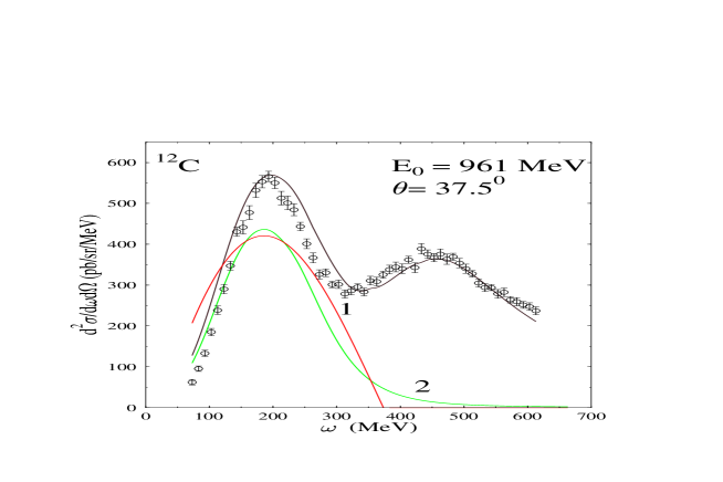
Figure 1: The quasi-elastic peak, 1 - free Fermi-gas, 2 - finite size nucleus. The upper line is the full calculation for nonrelativistic finite size nucleus including quasi-elastic, $\Delta$ , and MEC contributions

In the case of relativistic nucleon we have for the electromagnetic current density:

$$J_{\mu}(x)=\overline{\psi}(x)\Gamma_{\mu}\psi(x),$$

where

$$\Gamma_{\mu}=F_{1}\gamma_{\mu}-\frac{F_{2}}{2m}\sigma_{\mu\nu}q^{\nu}.$$

The Dirac formfactors $F_{1}$ and $F_{2}$ are related to the charge and magnetic formfactors by

$$F_{1}=\frac{F_{e}+\eta F_{m}}{1+\eta},\quad F_{2}=\frac{F_{m}-F_{e}}{1+\eta},\quad\eta=-\frac{q^{2}}{4m^{2}}.$$ (11)

For the Coulomb and the transversal responses we find then

$$R_{C}(\omega,{\bf q}^{2})=\frac{2}{(2\pi)^{3}}\int d^{3}p\Big{[}\frac{A({\bf q}^{2},\omega)}{\omega+q^{2}/2m-({\bf pq})/m}+\frac{A({\bf q}^{2},-\omega)}{-\omega+q^{2}/2m+({\bf pq})/m}\Big{]}$$ (12)

$$R_{T}(\omega,{\bf q}^{2})=\frac{2}{(2\pi)^{3}}\int d^{3}p\Big{[}\frac{A^{\prime}({\bf q}^{2},\omega)}{\omega+q^{2}/2m-({\bf pq})/m}+\frac{A^{\prime}({\bf q}^{2},-\omega)}{-\omega+q^{2}/2m+({\bf pq})/m}\Big{]},$$ (13)

where

$$A({\bf q}^{2},\omega)=\frac{F_{e}^{2}}{1+\eta}(1+\frac{\omega}{2m})^{2}+F_{m}^{2}\Big{[}\frac{\eta}{1+\eta}(1+\frac{\omega}{2m})^{2}-\frac{{\bf q}^{2}}{4m^{2}}\Big{]},$$ (14)

$$A^{\prime}({\bf q}^{2},\omega)=\frac{F_{e}^{2}+\eta F_{m}^{2}}{1+\eta}\cdot\frac{2}{m^{2}}\Big{[}{\bf p}^{2}-\frac{(m\omega+q^{2}/2)^{2}}{{\bf q}^{2}}\Big{]}-F_{m}^{2}\frac{q^{2}}{m^{2}}.$$ (15)

The Eqs. (12,13) were obtained assuming nonrelativistic motion of the nucleons inside the nucleus, putting thus $E_{\bf p}=m$ whenever it is possible. For this reason, we expect the difference between (12) and its nonrelativistic analog (9) to be mainly in kinematics. Comparing (9), (12) and (10), (13) we find the difference in the following. First, in the denominators of (9) and (10) we have to substitute $\omega\rightarrow\omega+\omega^{2}/2m$. Second, instead of simple formfactors squared we have the factors that are the combinations of the formfactors with some other factors depending on $\omega$ and $q^{2}$. These factors give the difference between Rosenbluth formula for the electron scattering cross-section from the proton and its nonrelativistic analog. It is worth to note that with these factors we have now the contribution to the Coulomb response from neutrons via the magnetic formfactor. At high momentum transfer this contribution is not negligible.

The substitution of $\omega$ is even more important. Due to this change the quasi-elastic peak is not broadening and keeps the correct peak position and the shape compared to the nonrelativistic response. In Fig.2 we see that the nonrelativistic response produces very broad quasi-elastic peak in comparison to the relativistic Fermi-gas response. This is not surprising because now we have the correct relativistic relation between the energy transfer and the particle-hole energy in the final state. After the substitution we have for the kinetic energy of outgoing nucleon the relation

$$T=\omega+\frac{\omega^{2}}{2m}.$$ (16)

Even if we use for the nucleon the nonrelativistic Schrödinger equation where $T={\bf p}^{2}/2m$, we obtain from (16) the correct relativistic relation between the energy-transfer $\omega$ and the momentum ${\bf p}$ of the nucleon in the continuum.

$$\omega=\sqrt{m^{2}+{\bf p}^{2}}-m.$$ (17)

So, the main effect of this substitution is pure kinematical. There is, however another effect. It is the presence of the negative energy intermediate states in the loop. However, in our region of $\omega<2m$ this part is real and does not contribute to the cross-section.

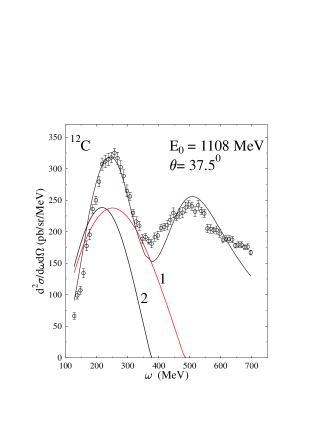
Figure 2: 1 - nonrelativistic Fermi-gas, 2 - relativistic Fermi-gas

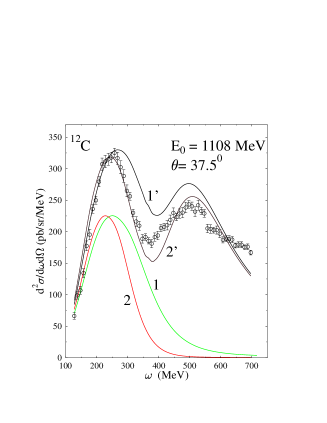
Figure 3: 1, 1’ - finite size nucleus, 2, 2’ - ”quasi-relativistic” finite size nucleus

Since the main effect has pure kinematical origin, we can try to extend our calculations for the finite size response functions to the region of high momentum transfer just by substituting $\omega$ in the argument of the Green functions in (6) by $\omega+\omega^{2}/2m$. This substitution will improve the energy-momentum relation for outgoing nucleons stabilizing, thus, the quasi-elastic peak. In Fig.3 we show the results of our calculations of the response functions for the finite size nucleus where we, first, substituted $\omega\rightarrow\omega+\omega^{2}/2m$, second, redefined the formfactors $F_{e}^{2}\rightarrow A({\bf q}^{2},\omega)$ for the Coulomb response and changed

$$F_{e}^{2}\to\frac{F_{e}^{2}+\eta F_{m}^{2}}{1+\eta},\;\;F_{m}^{2}\to F_{m}^{2}\Big{[}\frac{-q^{2}}{{\bf q}^{2}}\Big{]},$$ (18)

for the transversal response function. These last changes do not influence much the result, except for the Coulomb response of neutrons. The main effect comes from the improved kinematics. With these changes the result of finite size calculations does not differ much from the relativistic Fermi gas, except the low-energy wing of the quasi-elastic peak as it was found in [17]. One should keep in mind that the change (18) in the formfactors can be justified for the spin saturated nuclei only. For other nuclei one has to use the explicit relativistic corrections for the electromagnetic currents.

For a finite nucleus the response functions were calculated in the independent particles model where the particles were moving in the Woods-Saxon potential [21]

$$U(r)=(V+\imath W)f(r)+V_{ls}r_{0}^{2}({\bf ls})\frac{1}{r}\frac{df(r)}{dr}+V_{C}(r),$$ (19)

where

$$f(r)=\frac{1}{1+\exp{(r-R)/a}}.$$

The inclusion of the meson-exchange currents and the final state interaction for the outgoing nucleons leads to inevitable use of the optical potential for nucleons in the continuum [22]. In the region of the quasi-elastic peak we found the value of the imaginary part of the optical potential (19) $W=13$ MeV. This value is consistent with the parameters of the optical potential found in elastic proton scattering at the same proton energy [23].

The imaginary part of the optical potential brings an additional problem. It violates the conservation of the electromagnetic current. This nonconservation is very natural, since the imaginary part of the optical potential describes the flow of nucleons from single-particle to many-particle configurations. However, the amplitude of the process remains gauge invariant. In the amplitude the hadronic current is multiplied by the conserving electron electromagnetic current and the gauge dependent part of the amplitude, which is proportional to $q_{\mu}$, disappears. The Coulomb response function $S_{c}(w,{\bf q})$ depends explicitly now on both the charge density and the space-longitudinal part of the current density. However, we can redefine the hadronic current subtracting its 4-dimensionally longitudinal part

$$J^{\prime}_{\mu}=J_{\mu}-2\frac{q_{\mu}}{q^{2}}\cdot\Psi^{\dagger}({\bf r})W({\bf r})\Psi({\bf r})$$ (20)

For this corrected current we have the same expressions for the $S_{C}(\omega,{\bf q})$ via $J^{\prime}_{\mu}$ as given by (2).

3 $\Delta$-isobar excitation

The $\Delta$ - production contributes to the $S_{T}(\omega,{\bf q})$. The elementary amplitude of the $\Delta$ - production is given by [8]

$$T_{\gamma N,\Delta}(q^{2})=F_{N}(q^{2})\cdot(1+q^{2}/t^{2})\frac{f_{\gamma N,\Delta}}{m_{\Delta}}\sum\limits_{j}i[{\bf S}_{j}\times{\bf q}]T_{3j}e^{i{\bf qr}_{j}},$$ (21)

where $F_{N}(q^{2})$ is the usual nucleon electromagnetic formfactor, and $t=6GeV/c$. The coupling constant $f_{\gamma N,\Delta}$=3.6 was found from the reaction on a single proton [8]. ${\bf S}$ and ${\bf T}$ are the spin and the isospin transition matrices.

For a spherical nucleus it is convenient to use the multipole expansion

$$[{\bf S}_{j}\times{\bf q}]_{\nu}e^{\imath{\bf qr}}=4\pi\sum\limits_{JLM}(i)^{L}\j_{L}(qr)({\bf S}\cdot{\bf Y}^{L}_{JM}(\hat{\bf n}))[{\bf Y}_{JM}^{L\ast}(\hat{\bf q})\times{\bf q}]_{\nu}$$ (22)

where ${\bf Y}_{JM}^{L}({\bf n})$ is the vector spherical function. The multipole transition density in terms of the tensor operators (22) is defined by

$$\rho^{L}_{JM}(r)=\sum\limits_{j}({\bf S}\cdot{\bf Y}_{JM}^{L}({\bf n}))T_{3j}\frac{\delta(r-r_{j})}{r^{2}}$$ (23)

The structure function $S_{T}(\omega,{\bf q})$ can be presented then as a sum of contributions from different multipoles

$$S_{T}(\omega,{\bf q})=F^{2}_{N}(q^{2})(1+q^{2}/t^{2})^{2}\frac{4\pi F^{2}_{\gamma N\Delta}(q^{2})}{m^{2}_{\Delta}}\sum\limits_{J=0}^{\infty}[(J+1)W^{J}_{J-1J-1}(\omega,q)+$$

$$JW^{J}_{J+1J+1}(\omega,q)-\sqrt{J(J+1)}W_{J-1J+1}^{J}(\omega,q)-$$

$$\sqrt{J(J+1)}W^{J}_{J+1J-1}(\omega,q)+(2J+1)W^{J}_{JJ}(\omega,q)],$$ (24)

where $W^{J}_{LL^{\prime}}(\omega,q)$ is the diagonal Fourie component of the imaginary part of the response function

$$W^{J}_{LL^{\prime}}(\omega,q)=-\frac{1}{\pi}\int_{0}^{\infty}r^{2}drj_{L}(qr)ImR_{LL^{\prime}}^{J}(r,r^{\prime};\omega)j_{L^{\prime}}(qr^{\prime})r^{{}^{\prime}2}dr^{\prime},$$ (25)

$$\delta_{JJ^{\prime}}\delta_{MM^{\prime}}R^{J}_{LL^{\prime}}(r,r^{\prime};\omega)=<i|\rho^{{\dagger}L}_{JM}(r)\frac{1}{\omega-E_{i}-H+i\delta}\rho^{L^{\prime}}_{J^{\prime}M^{\prime}}(r^{\prime})|i>.$$ (26)

The many-body hamiltonian $H$ in (26) includes the $\Delta$ - nucleus and nucleon - nucleus single particle hamiltonians together with free $\Delta$ width and the $\Delta-N$ and $N-N$ residual interactions.

$$H=h_{\Delta}-i\Gamma_{\Delta}/2+\sum\limits^{A-1}_{j=1}\sum\limits^{A-1}_{j=1}V_{\Delta N}(r_{\Delta}-r_{j})+\frac{1}{2}\sum\limits^{A-1}_{i\neq j}V_{NN}(r_{i}-r_{j})$$ (27)

The transition density operator (23) acting on ground nuclear state creates a $\Delta$ - hole state. Using this set of states and neglecting the residual interaction one can obtain the following expression for the response function (26)

$$R^{J}_{LL^{\prime}}(r,r^{\prime};\omega)=\frac{2}{3}\frac{1}{2J+1}\times$$

$$\sum\limits_{\nu_{\Delta}\nu_{h}}n_{\nu_{h}}\frac{<\nu_{h}\|{\bf S}^{\dagger}\cdot{\bf Y}^{L*}_{J}\|\nu_{\Delta}><\nu_{\Delta}\|{\bf S}\cdot{\bf Y}_{J}^{L}\|\nu_{h}>R^{*}_{\nu_{h}}(r)R_{\nu_{\Delta}}(r)R^{*}_{\nu_{\Delta}}(r^{\prime})R_{\nu_{h}}(r^{\prime})}{\omega+\epsilon_{\nu_{h}}-\epsilon_{\nu_{\Delta}}-\Delta m+i\Gamma_{\Delta}(\omega)/2}$$ (28)

where $\epsilon_{\nu}$ and $R_{\nu}(r)$ are the single-particle energies and the wave functions of the $\Delta$ and the bounded nucleons. In (28) we neglected the contribution of the backward loop because it has large energy denominator, of the order of $2\Delta m$, and it does not have the imaginary part at all.

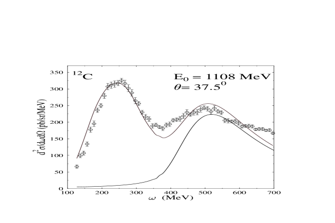
Figure 4: The $\Delta$-isobar contribution

In order to calculate the response function (28) of a finite nucleus it is convenient to define the Green function of the single-particle radial equation for a $\Delta$

$$G_{J_{\Delta}l_{\Delta}}(r,r^{\prime};\epsilon)=\sum\limits_{n_{\Delta}}\frac{R_{n_{\Delta}j_{\Delta}l_{\Delta}}(r)R^{*}_{n_{\Delta}j_{\Delta}l_{\Delta}}(r^{\prime})}{\epsilon-\epsilon_{n_{\Delta}j_{\Delta}l_{\Delta}}+i\Gamma(\epsilon)/2}$$ (29)

that satisfies the equation

$$(\epsilon-\stackrel{{\scriptstyle\land}}{{h}}_{j_{\Delta}l_{\Delta}})G_{j_{\Delta}l_{\Delta}}(r,r^{\prime};\epsilon)=\delta(r-r^{\prime}),$$ (30)

where $\stackrel{{\scriptstyle\land}}{{h}}_{j_{\Delta}l_{\Delta}}$ is the radial $\Delta$ - nucleus Hamiltonian. The asymptotic behavior of the $G_{j_{\Delta}l_{\Delta}}(r,r^{\prime};\epsilon)$ at large $r,r^{\prime}$ is determined by a pole position in (29).

$$G_{j_{\Delta}l_{\Delta}}(r,r^{\prime})\sim\exp(ikr),$$ (31)

where $k=\sqrt{2m_{\Delta}/\hbar^{2}(\epsilon+i\Gamma/2)}$. The expression for the response function (28) becomes

$$R^{J}_{LL^{\prime}}(r,r^{\prime};\omega)=\frac{1}{2}\frac{1}{2J+1}\sum\limits_{\nu_{\Delta}\nu_{h}}n_{\nu_{h}}<\nu_{h}\|{\bf S}^{\dagger}\cdot{\bf Y}^{L*}_{J}\|\nu_{\Delta}><\nu_{\Delta}\|{\bf S}\cdot{\bf Y}^{L}_{J}\|\nu_{h}>\times$$

$$G_{j_{\Delta}l_{\Delta}}(r,r^{\prime};\omega-\Delta m+\epsilon_{\nu_{h}}).$$ (32)

The $\Delta$-nucleus optical potential has been taken in the Woods-Saxon form with the parameters found from the pion-nucleus data [24] The results of the calculations of the $\Delta$-isobar contribution into inclusive spectrum for the electron scattering from ${}^{12}C$ at the energy of incident electron 1108 MeV are shown in the Fig.4.

4 Meson-exchange currents

It is known that the single-nucleon and single-$\Delta$ degrees of freedom do not exhaust the spectrum especially in the intermediate region between N and $\Delta$ peaks. The meson-exchange currents are necessary to account for quantitative description of the spectra [25, 26]. Part of the MEC has been included already into the $\Delta$-excitation process. Here we shall discuss only the nucleon sector of MEC.

As it can be inferred from [25] there are three types of diagrams shown in Fig.5. This diagrams correspond to the following expressions for the current densities:

$$J_{\mu}^{\pi-in-fl}=2iP_{\mu}\;({\bf P}-{\bf q}/2)\cdot\mbox{\boldmath$\sigma$}_{11^{\prime}}\;({\bf P}+{\bf q}/2)\cdot\mbox{\boldmath$\sigma$}_{22^{\prime}}\cdot$$

$$[\mbox{\boldmath$\tau$}_{1}\times\mbox{\boldmath$\tau$}_{2}]_{3}\cdot\frac{f_{\pi}(P-q/2)\cdot f_{\pi}(P+q/2)}{({m_{\pi}}^{2}-(P+q/2)^{2})({m_{\pi}}^{2}-(P-q/2)^{2})},$$ (33)

Fig.5 (c), which is usually called the pion-in-flight contribution.

$$J_{\mu}^{cont}=i[\overline{U}(P_{2}^{\prime})(\hat{P}+\hat{q}/2)\gamma_{5}U(P_{2})\,\overline{U}(P_{1}^{\prime})\gamma_{\mu}\gamma_{5}U(P_{1})\,[\mbox{\boldmath$\tau$}_{1}\times\mbox{\boldmath$\tau$}_{2}]_{3}\cdot$$

$$\frac{{f_{\pi}}^{2}(P+q/2)}{({m_{\pi}}^{2}-(P+q/2)^{2})}+\overline{U}(P_{1}^{\prime})(\hat{P}-\hat{q}/2)\gamma_{5}U(P_{1})\,\overline{U}(P_{2}^{\prime})\gamma_{\mu}\gamma_{5}U(P_{2})\,[\mbox{\boldmath$\tau$}_{1}\times\mbox{\boldmath$\tau$}_{2}]_{3}$$

$$\cdot\frac{{f_{\pi}}^{2}(P-q/2)}{({m_{\pi}}^{2}-(P-q/2)^{2})}]$$ (34)

Figure 5: Meson-exchange currents diagrams

Fig.5 (b), which is called the contact contribution, and

$$J_{\mu}^{prop}=[\overline{U}(P_{1}^{\prime})\gamma_{\mu}\frac{1}{(m-(\hat{P}_{1}^{\prime}-\hat{q}))}\gamma_{\nu}\gamma_{5}U(P_{1})\cdot\overline{U}(P_{2}^{\prime})\gamma_{\kappa}\gamma_{5}U(P_{2})\cdot$$

$$\cdot(P+q/2)^{\nu}(P+q/2)^{\kappa}\cdot\frac{1}{2}(1+\tau_{3}^{(1)})\mbox{\boldmath$\tau$}^{(1)}\cdot\mbox{\boldmath$\tau$}^{(2)}+$$

$$+\overline{U}(P_{1}^{\prime})\gamma_{\nu}\gamma_{5}\frac{1}{(m-(\hat{P}_{1}+\hat{q}))}\gamma_{\mu}U(P_{1})\cdot\overline{U}(P_{2}^{\prime})\gamma_{\kappa}\gamma_{5}U(P_{2})\cdot$$

$$(P+q/2)^{\nu}(P+q/2)^{\kappa}\cdot\mbox{\boldmath$\tau$}^{(1)}\cdot\mbox{\boldmath$\tau$}^{(2)}\frac{1}{2}(1+\tau_{3}^{(1)})]\cdot\frac{{f_{\pi}}^{2}(P+q/2)}{({m_{\pi}}^{2}-(P+q/2)^{2})}+$$

$$+[1\leftrightarrow 2,q\leftrightarrow-q]\cdot\frac{{f_{\pi}}^{2}(P-q/2)}{({m_{\pi}}^{2}-(P-q/2)^{2})}$$ (35)

Fig.5 (a), which is the propagation contribution. The factor $f_{\pi}(P)$ is a pion formfactor and it was taken as in [25]

$$f_{\pi}(p)=(\Lambda^{2}-m_{\pi}^{2})/(\Lambda^{2}-p^{2})$$

.

In our calculations the best agreement with the data was obtained for $\Lambda$ = 1250 MeV.

The total current, which is the sum of these three terms $J_{\mu}=J_{\mu}^{\pi-in-fl}+J_{\mu}^{cont}+J_{\mu}^{prop}$ , is really conserving.

Let us discuss the diagram (a) more closely. Here we have two different situations for the positive and the negative energy states in the propagator of nucleons. We would like to note, that the diagrams have a pole in the region of the quasi-elastic peak and we inevitably cross it during the integration over the initial momentum of the nucleon. This singularity produces infinite contribution to the cross-section. The way of treating this singularity in given order of perturbation theory has been indicated in [19]. We would like to use different approach in the interpretation of the pole. Let us remark that the pion-exchange is not specific in this diagram and it can be replaced by any other interaction. The pole in the diagrams does not disappear. One can immediately draw the higher order diagrams, where the singularity will be accumulating. As it was shown in [22], this kind of diagrams corresponds to the interaction in final state for the positive energy states of propagating nucleon. Summing these diagrams we come to the optical potential for the final state nucleons and the contribution of the diagrams (a) for the intermediate states with positive energy should be omitted at all if we use an optical potential in order to avoid double counting.

As for negative energy intermediate states, it was shown in [26] that their contribution is small and we neglect it here as well.

In order to calculate the cross-section we have to square the obtained currents and to integrate them over three momenta $P$, $P_{1}$, and $P_{2}$. The simplest way to do it is to calculate the corresponding response functions as it has been done for the single-nucleon channel. The diagrams for the response functions are presented in Fig.6. It is seen clearly that the integration over the momenta is almost factorized. We have separate integration in the upper loop over ($P_{1}$), in the lower loop over ($P_{2}$), and over the momentum carried by the pion ($P$).

Figure 6: Loops for MEC

The calculations of the particle-hole loop for the pion channel have been done in [28]. We need to compute the upper loops only. The result is: for the diagram (a)

$$R^{()}_{up}(\omega,{\bf q},P)=\frac{2}{(2\pi)^{3}}\int d^{3}P_{1}\Big{[}\frac{A({\bf q},\omega,P,P_{1})}{\omega+P_{0}+(q+P)^{2}/2m-({\bf P_{1}}\cdot{\bf(q+P)})/m}-$$

$$-\frac{A({\bf q},\omega,P,-P_{1})}{\omega+P_{0}-(q+P)^{2}/2m-({\bf P_{1}}\cdot{\bf(q+P)})/m}\Big{]},$$ (36)

where

$$A({\bf q},\omega,P,P_{1})=4\Big{[}(2m^{2}+P_{1}\cdot(q-P))\cdot(g_{\mu\nu}-\frac{q_{\mu}q_{\nu}}{q^{2}})-$$

$$-2(P_{1\mu}-\frac{q_{\mu}(qP_{1})}{q^{2}})\cdot(P_{1\nu}-\frac{q_{\nu}(qP_{1})}{q^{2}})+(P_{1\mu}-\frac{q_{\mu}(qP_{1})}{q^{2}})\cdot(P_{\nu}-\frac{q_{\nu}(qP)}{q^{2}})+$$

$$+(P_{\mu}-\frac{q_{\mu}(qP)}{q^{2}})\cdot(P_{1\nu}-\frac{q_{\nu}(qP_{1})}{q^{2}})$$ (37)

Here $A({\bf q},\omega,P)$ is written in a symbolic form both for the Coulomb and the transversal responses.

For (b) we obtain

$$R^{(b)}_{up}(\omega,{\bf q},P)=\frac{2}{(2\pi)^{3}}\int d^{3}P_{1}\Big{[}\frac{B({\bf q},\omega,P,P_{1})}{\omega+P_{0}+(q+P)^{2}/2m-({\bf P_{1}}\cdot{\bf(q+P)})/m}-$$

$$-\frac{B({\bf q},\omega,P,-P_{1})}{\omega+P_{0}-(q+P)^{2}/2m-({\bf P_{1}}\cdot{\bf(q+P)})/m}\Big{]},$$ (38)

where

$$B({\bf q},\omega,P,P_{1})=4\Big{[}2m^{2}\cdot(P_{\mu}-\frac{q_{\mu}(qP_{)}}{q^{2}})(2P_{\nu}-q_{\nu})+$$

$$+(P_{1\mu}-\frac{q_{\mu}(qP_{1})}{q^{2}})(2P_{\nu}-q_{\nu})\cdot({(q-P)}^{2}+2\cdot P_{1}(q-P))\Big{]}$$ (39)

Using the above expressions for the response functions we obtain

$$R_{C,T}(\omega,{\bf q})=4\int\frac{d^{4}P}{(2\pi)^{4}}\Big{[}2R^{()}_{up}(\omega,{\bf q},P)R^{()}_{low}(\omega,{\bf q},P)\cdot\frac{{f_{\pi}(P)}^{4}}{{(P^{2}-{m_{\pi}}^{2})}^{2}}+$$

$$+2R^{(b)}_{up}(\omega,{\bf q},P)R^{(b)}_{low}(\omega,{\bf q},P)\cdot\frac{{f_{\pi}(P)}^{2}{f_{\pi}(q-P)}^{2}}{(P^{2}-{m_{\pi}}^{2})({(q-P)}^{2}-{m_{\pi}}^{2})}+$$

$$+4R^{(c)}_{up}(\omega,{\bf q},P)R^{(c)}_{low}(\omega,{\bf q},P)\cdot\frac{{f_{\pi}(P)}^{3}f_{\pi}(q-P)}{{(P^{2}-{m_{\pi}}^{2})}^{2}({(q-P)}^{2}-{m_{\pi}}^{2})}+$$

$$+R^{(d)}_{up}(\omega,{\bf q},P)R^{(d)}_{low}(\omega,{\bf q},P)\cdot\frac{{f_{\pi}(P)}^{2}{f_{\pi}(q-P)}^{2}}{{(P^{2}-{m_{\pi}}^{2})}^{2}{({(q-P)}^{2}-{m_{\pi}}^{2})}^{2}}\Big{]}$$ (40)

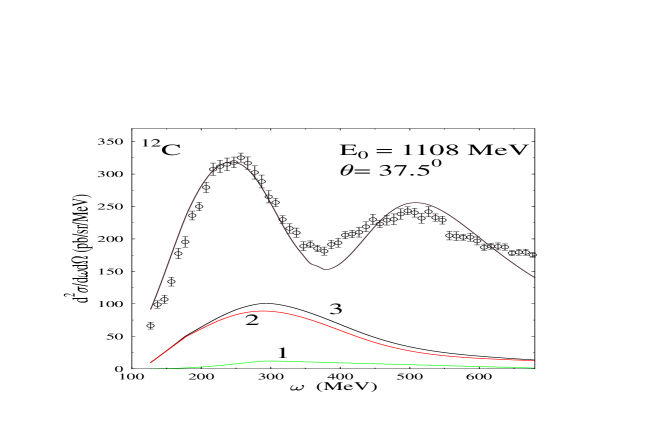
Figure 7: 1 - the longitudinal cross-section, 2 - the transversal cross-section, 3 - the total cross-section from the meson-exchange currents

The contribution of each response function is shown in Fig.7. As in the previous calculations the transversal response is considerably larger than the longitudinal response [27].

In general, at high momentum transfer the contribution of the meson-exchange currents is considerable and can not be neglected.

5 Results for ${}^{12}C$ and ${}^{16}O$

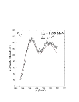
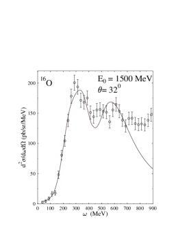
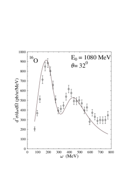
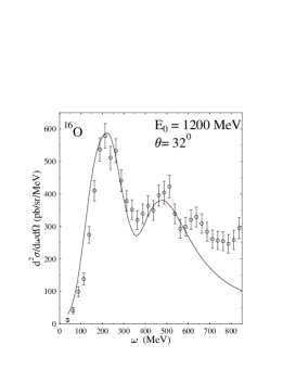
Figure 8: Total cross-section including quasi-elastic peak, $\Delta$ - excitation and MEC

The final results of our approach are shown in Fig.8, where we present the spectra at high electron energy for two nuclei ${}^{12}C$ and ${}^{16}O$ [7, 8]. For both nuclei the calculations were performed with the same set of the parameters (except the size of a nucleus). Again, the best fit was obtained to the data with the highest momentum transfer, Fig.8. At lower momentum transfer, Fig.1 and Fig.2, there is a small systematic shift of the quasi-elastic peak position. This can be indication that either some 1p-1h correlations still present in the final state even at this high momentum transfer, or it can be the difference in the potential depths for the bounded nucleons and the nucleons in the continuum. The oxigen data show the large contribution to the cross-section behind the $\Delta$-peak. This is the indication of higher nucleon resonances excitation. However, just the number of MEC diagrams is much larger in this region and they can hide the resonance contribution. This problem needs separate investigation.

In conclusion, we calculated the inclusive cross-section in the regions of quasi-elastic peak, $\Delta$ - peak and the intermediate region. It was demonstrated that in accordance with the earlier calculations the nonrelativistic approach fails to reproduce the shape of quasi-elastic peak at high momentum transfer and the simple recipe was proposed to account the relativistic kinematics for the finite nucleus calculations.

6 Acknowledgment

The encouraging discussions with T.-S.H. Lee on the initial stage of work are greatly acknowledged by one of the author (V.D.) The authors are grateful to Dr. M.Anghinolfi for presenting the oxygen data.

References

- [1] P. Barreau et al., Nucl. Phys. A402 (1983) 515.
- [2] Z.E. Meziani et al., Phys. Rev. Lett. 52 (1984) 2180.
- [3] J.S. O’Connell et al., Phys. Rev. Lett. 53 (1984) 1627.
- [4] Z.E. Meziani et al., Phys. Rev. Lett. 54 (1985) 1233.
- [5] D.T. Baran et al., Phys. Rev. Lett. 61 (1988) 400.
- [6] R.M.Sealock et al., Phys. Rev. Lett. 62 (1989) 1350.
- [7] J.S. O’Connell and R.M. Sealock, Phys. Rev. C 42 (1990) 2290.
- [8] M. Anghinolfi et.al., Nucl. Phys. A602 (1996),405.
- [9] S. Boffi, C. Guisti and F.D. Pacati, Phys. Rep. 226C (1993) 1.
- [10] J. Jourdan, Phys. Lett., B353 (1995) 189.
- [11] R.Cenni, F.Conte, P.Saracco, nucl-th/9702026, submitted to Nucl. Phys. A.
- [12] W.M. Alberico et al., Phys. Rev. C 38 (1988) 1801.
- [13] M. Kohno and N. Ohtsuka, Phys. Lett. 98B (1981) 335.
- [14] C.R. Chen and T.-S. H. Lee, Phys. Rev. C 38 (1988) 2187.
- [15] C. J. Horowitz and J. Piekarewicz, Nucl. Phys. A511 (1990) 461.
- [16] J. D. Walecka, Ann. of Phys. 83 (1974) 491.
- [17] J.E. Amaro et al., Nucl. Phys. A602 (1996) 263.
- [18] T.W.Donelly, J.D.Walecka, Ann. Rev. Nucl. Sci., 25 (1975) 329.
- [19] W.M. Alberico et al., Nucl. Phys. A512 (1990) 541.
- [20] M.J. Dekker, P.J. Brussaard and J.A. Tjon, Phys. Lett. B 289 (1992) 255.
- [21] A.Bohr, B.Mottelson, Nuclear Structure (v.1), W.A. Benjamin Inc. NY,Amsterdam. (1969).
- [22] Y.Horikawa, F.Lenz, Nimai C.Mukhopadhyay Phys. Rev. C, 22 (1980) 1680.
- [23] H.Fiedeldey and C.A. Engelbrecht, Nucl. Phys. A128 (1968) 673.
- [24] Y. Horikawa, M. Thies, and F. Lenz, Nucl. Phys. A345 (1980) 386.
- [25] D.O.Riska, Phys. Rep. C 181 (1989) 207.
- [26] J.W. Van Orden and T.W. Donnelly, Ann. of Phys., 131 (1981) 451.
- [27] J. Ryckebusch, M. Vanderhaeghen, L. Machenil, M. Waroquier, Nucl. Phys. A568 (1994) 820.
- [28] V.F.Dmitriev and Toru Suzuki, Nucl. Phys., A438, 1985.