Sensitivity of the deuteron form factor to nucleon resonances^∗

Abstract

The sensitivity of the deuteron form factor to contributions from the excited states of the nucleon is explored using a simple model of the nucleon-nucleon interaction which employs a tower of charged nucleon resonances. The model is manifestly covariant, analytically solvable, and gauge invariant. The consequences of this model are studied in the simplest possible framework. We assume that all particles have spin zero and that the tower has only three charged members, which consist of the proton, the Roper, and a higher state in the vicinity of the ${D}_{13}$. Nucleon-nucleon $S$-wave phase shifts and the deuteron form factor are calculated using this three member tower, and the results are compared to similar calculations using the proton ground state only. We conclude that the deuteron form factor is insensitive to the presence of excited states of the proton unless those states are of sufficiently low mass to produce strong inelasticities in $NN$ scattering channels.

I Overview, results, and conclusions

A Introduction

Now that first results from experiments performed at the Thomas Jefferson National Accelerator Facility (Jefferson Lab) are becoming available, the details of the two nucleon current may be explored in great detail. Some of the new experiments will probe the short range structure of this current, which can be interpreted as arising from the exchange of quarks and gluons, or alternatively, from meson exchange and the excitation of virtual excited states of the nucleons. In this paper we turn our attention to virtual contributions from these nucleon excited states.

The effects of nucleon resonances (or excited states) are obvious above the production threshold; it is less obvious what effect they will have on cross sections and observables measured well below the production threshold. Denoting the mass of the final state in electron scattering by $M_{x}$, and the square of the four momentum transfer by $Q^{2}>0$, we try to answer the following question: “If $M_{x}$ lies below the threshold for the physical excitation of nucleon resonances, does their existance nevertheless affect the high $Q^{2}$ behavior of form factors and structure functions?” To study this question we introduce the “tower of states” model. This is a simple, dynamical model for the study of nucleon resonances which can make easy, but admittedly rough, predictions of the effects that might be seen at places like Jefferson Lab. The goal is to use this simple model to get a qualitative feeling of where effects due to resonances will be large.

Any such model must be compatible with highly successful theories of $NN$ interactions [3] –[11] which have gone before. Motivated by previous work [11] and the relativistic work of Tjon and collaborators [12] –[15] we use manifestly covariant dynamics. When working at the level of a few GeV, as at Jefferson Lab, one must use relativistic equations. The model is constructed so that gauge invariance is satisfied exactly. This requires the introduction of an interaction current which is derived from the strong kernel. Finally, the model is analytically solvable, allowing for simple calculations of various properties of the $NN$ system. Many of these features have appeared in earlier models, but, to our knowledge, this is the first time the contributions from resonances and their corresponding interaction currents have been systematically applied to the study of the deuteron form factor using a simple model which is analytically solvable, covariant, and gauge invariant.

In this first study we use the simplest possible potential (rank-one separable), with a minimal number of free parameters (five, at most). We fix all free parameters by fitting the $NN$ phase shifts below lab energies of 350 MeV. All deuteron properties (binding energy, wavefunctions, form factors) are then calculated from the model. Our treatment of the nucleon resonances varies somewhat from earlier works. Most models have considered the addition of only one additional resonance, usually the $\Delta$ (Ref. [6] is an exception, however, but see the discussion in Ref. [15]). Such channels have been considered as add-ons to existing successful $NN$ models [9], or used to increase the applicability of such models [15]. Previous calculations of the deuteron form factor using separable models have usually ignored the interaction current which should accompany the calculation. The philosophy behind our treatment is that the resonances and their interaction currents should be consistently included on an equal footing from the beginning.

Since we wish to keep this first exploration of the contribution of resonances as simple as possible, we have neglected spin (all particles in the following discussions are scalar), and used a basic separable four-point interaction diagram as the kernel with a “tower” consisting of only three states. A Tabakin-style form factor, similar to the one used by Rupp and Tjon [16], is employed in order to realistically model the contributions of meson exchange without actually having to deal with its complexities. We compare results from a three member tower with those obtained from a purely elastic scattering model (a one member tower, in our language). Therefore, any differences between the models which include higher resonances and those which do not are due to the presence of the resonances. Clearly, if differences between these models can be seen even at this basic level, then further investigation with more complicated systems is warranted.

In this section we begin with an overview of the techniques used in formulating the model, and then discuss the results of this work. Particular attention is paid to the effects of inelasticity on the tower models. At the end of this section we present our conclusions. Sec. II includes a full development of the model, including the solution of the relativistic scattering equation, proof of unitarity, a proof of gauge invariance, and the development of the deuteron form factor. The relations used for inelastic scattering are also derived. In order to maintain gauge invariance, contributions from an interaction current are required, since the kernel of the this model is dependent on the center-of-mass four-momentum. The interaction current is fully derived in the Appendix, and the contributions from the interaction current prove to be very important to several facets of the $NN$ system. Finally, Sec. III includes some specific details of the models.

B Background and overview

The tower of states model is built upon the idea that, in the process of repeated scattering with a neutron, a proton may “sample” any one of its higher order resonances (the “tower”). That is, the proton and neutron interact, causing the proton to become a virtual Roper for a short period of time before interacting again with the neutron. In successive scatterings, multiple samplings of this tower of higher resonant states could occur. We explore the effects that such sampling will have on various properties of the $NN$ system, particularly the properties of the deuteron where all inelastic contributions are virtual.

As a brief overview of the techniques used in formulating the model, we begin with the most general form of the relativistic scattering equation

$$M={\cal V}+\int_{k}{\cal V}GM,$$ (1)

where ${\cal V}$ is the relativistic kernel, G is the propagator, and $\int_{k}$ is specified by choosing a particular formalism, such as Bethe-Salpeter [17], Blankenbecler-Sugar [18], or Spectator [19]–[22]. The basic four-point interaction between a member of the tower and a neutron shown in Fig. 1 is chosen as the kernel. The coupling strengths are denoted by the coupling matrix $g_{ij}$, where $i$ and $j$ denote members of the tower. We include a Tabakin-style form factor

$$f(x)=\frac{(\alpha^{2}-x)(p_{c}^{2}+x)}{(\gamma^{2}-x)(\beta^{2}-x)^{2}},$$ (2)

with

$$x=x(p,P)={p}^{2}-\frac{(P\cdot{p})^{2}}{P^{2}},$$ (3)

where ${p}$ is the relative momentum between the neutron and the tower member and $P$ is the center of mass four-momentum (for a detailed definition of the form factor, see Sec. III A). As shown by Rupp and Tjon [16], and again here for a one-member tower called Model 1, the Tabakin form factor allows one to successfully model the $NN$ system without having to actually perform meson exchange calculations. Since spin is being neglected at this time, all particles have scalar propagators. Finally, we choose to work in the spectator formalism [19]–[22], which has proven to be very useful in describing the $NN$ system [11], [20]. For simplicity in this first treatment, we will treat the $np$ system only, and discard the isospn formalism, so that the neutron and proton are nonidentical particles. The spectator formalism is then simplified if the neutral particle, i.e. the neutron, is placed consistently on its mass shell and excluded from the tower of states. The towers will contain the proton and its charged excited states only.

FIG. 1.: Basic tower of states interaction. This diagram forms the kernel of the spectator equation describing the scattering and bound states of the system. The cross on the neutron lines denotes that the particle is on the mass shell.

These choices are not made arbitrarily. Each has been specifically chosen to reduce the complexity of the system in some way without losing the essential physics. By constructing a very basic, separable kernel, the $M$-matrix may be obtained analytically (see Sec. II for the full details). Neglecting spin is, of course, an automatic reduction of complexity useful for this first treatment of the problem. The choice of the spectator formalism motivates the initial inclusion of only one tower (since one particle is on shell, it is natural to restrict it to its ground state, although a more complete treatment can be developed later) and is chosen because it is easily extended to more complex cases. Finally, treating the proton and neutron as nonidentical particles and neglecting the distribution of charge inside the neutron allows us to restrict the electromagnetic interaction to the tower members; the neutron does not interact with the photon in the naive models considered here.

FIG. 2.: The basic electromagnetic coupling between tower members

Once the scattering equation has been solved, we obtain the $S$-wave phase shifts, $\delta$, and inelasticity parameters, $\eta=\cos\rho$, from the usual representation of the inelastic scattering amplitude

$$-{M}=\frac{\eta e^{2i\delta_{1}}-1}{2i\rho_{1}}\,,$$ (4)

where $\rho_{1}$ (not to be confused with the inelastic phase angle $\rho$) is the relativistic phase space factor given in Eq. (26) below. The free parameters of the models are then fit to the Nijmegen 1993 phase shifts below 350 MeV [23]. Excellent fits are obtained using towers with either one or three members. Fits using a two member tower were attempted, but proved to be less successful than those obtained from one- and three-member towers. The reason for these poor fits is under investigation; it may be related to the need for a certain symmetry between the coupling constants. Due to the larger number of free parameters, $\chi^{2}$s for three-member tower models are slightly improved over those using only the proton. These results will be presented in Sec. I C.

In order to explore the effect of the resonances in a simple $NN$ system where they can can only make virtual contributions, we study the deuteron form factor. The electromagnetic coupling between tower members, illustrated in Fig. 2, is chosen to be proportional to $e_{ij}=\zeta_{ij}e$, where $e$ is the electric charge. The full currents with electromagnetic form factors are constructed using the methods of Gross and Riska [24] (see Eq. (40) for more detail). In this simple first treatment we choose $\zeta_{ij}=\delta_{ij}$ so the photon itself cannot excite or de-excite members of the tower. In order to satisfy gauge invariance an interaction current must be included, and the inclusion and study of this current is one of the novel features of this work. This current is derived from the kernel ${\cal V}$ by minimal substitution using the methods of Ito et. al. [25]. However, because the structure of the kernel is different from the one assumed by Ito et. al., a slightly different argument is needed, and because the derivation is somewhat lengthly the details are presented in the Appendix.

C Numerical results

From the real and imaginary parts of $M$ we calculate the phase shifts and perform a least-squares fit to fix the free parameters in the models. The resulting parameters for three models are shown in Table I. Model 1 consists of a tower with the proton only, Model 3 employs a three-member tower consisting of the proton, Roper, and ${\rm D}_{13}$, and Model 3I uses the same three-member tower, except that the mass of the Roper has been lowered to increase its inelastic contributions. The inelastic region has no effect on the fitting procedure, as only data below 350 MeV are used in the fit.

TABLE I.: Parameters in the tower of states models. Numbers in bold face were varied during the fitting procedure. The form factor parameters and all masses are in GeV; all the coupling constants have dimensions ${\rm GeV}^{4}$.

	Model 1		Model 3		Model 3I
Parameter	${}^{1}S_{0}$	${}^{3}S_{1}$	${}^{1}S_{0}$	${}^{3}S_{1}$	${}^{1}S_{0}$	${}^{3}S_{1}$
$\alpha$	0.198125	0.155094	0.197611	0.157080	0.197750	0.150054
$\beta$	1.09772	1.27872	1.09795	1.29825	1.10168	1.28994
$\gamma$	0.171623	0.136404	0.172138	0.139047	0.172141	0.129887
$p_{c}$	0.3492	0.412689	0.3492	0.412689	0.3492	0.412689
$g_{11}$	-1516.96	-2553.31	-1500.89	-2615.86	-1504.81	-2554.04
$g_{12}$			155.0	406.731	190.0	404.563
$g_{13}$			155.0	-105.0	190.0	-105.0
$g_{22}$			10.0	-105.0	15.0	-105.0
$g_{23}$			272.175	597.206	253.928	591.489
$g_{33}$			10.0	-105.0	15.0	-105.0
$\chi^{2}$	6.97	7.60	5.06	6.83	3.66	6.04
$m_{1}$	0.93825		0.93825		0.93825
$m_{2}$			1.44		1.17
$m_{3}$			1.52		1.52

TABLE II.: Binding energy of the deuteron as calculated in each of the three models. The percent error shown is the error between the calculated value and the expected value of 2.22 MeV. The energies are given in MeV.

	Model 1	Model 3	Model 3I
Binding Energy	2.15	2.02	2.47
Percent Error	3.2	9.0	11.3

TABLE III.: Values for the phase shifts, in degrees, below 350 MeV. $T_{{\rm LAB}}$ is in MeV.

	Nijmegen 1993a		Model 1		Model 3		Model 3I
$T_{{\rm LAB}}$	${}^{1}S_{0}$	${}^{3}S_{1}$	${}^{1}S_{0}$	${}^{3}S_{1}$	${}^{1}S_{0}$	${}^{3}S_{1}$	${}^{1}S_{0}$	${}^{3}S_{1}$
$1$	$62.029$	$147.75$	$61.559$	$147.97$	$60.889$	$147.58$	$61.2$	$148.36$
$5$	$63.627$	$118.18$	$64.203$	$118.27$	$63.99$	$117.83$	$64.148$	$118.54$
$10$	$59.956$	$102.61$	$60.55$	$102.32$	$60.498$	$101.96$	$60.614$	$102.35$
$25$	$50.903$	$80.629$	$51.199$	$80.009$	$51.32$	$79.786$	$51.403$	$79.705$
$50$	$40.545$	$62.767$	$40.675$	$62.641$	$40.884$	$62.468$	$40.961$	$62.222$
$75$	$32.933$	$51.585$	$32.912$	$51.852$	$33.149$	$51.685$	$33.232$	$51.435$
$100$	$26.783$	$43.227$	$26.564$	$43.72$	$26.812$	$43.556$	$26.903$	$43.332$
$125$	$21.549$	$36.46$	$21.174$	$37.146$	$21.423$	$36.985$	$21.525$	$36.793$
$150$	$16.939$	$30.72$	$16.371$	$31.480$	$16.618$	$31.327$	$16.73$	$31.165$
$175$	$12.776$	$25.701$	$12.075$	$26.536$	$12.317$	$26.394$	$12.439$	$26.258$
$200$	$8.943$	$21.216$	$8.08$	$22.026$	$8.3152$	$21.898$	$8.4471$	$21.786$
$225$	$5.357$	$17.14$	$4.4249$	$17.959$	$4.648$	$17.847$	$4.7894$	$17.755$
$250$	$1.959$	$13.386$	$1.031$	$14.189$	$1.2076$	$14.095$	$1.3552$	$14.022$
$275$	$-1.3$	$9.89$	$-2.3423$	$10.696$	$-2.0353$	$10.621$	$-1.8673$	$10.565$
$300$	$-4.457$	$6.602$	$-5.3305$	$7.4381$	$-5.0731$	$7.3836$	$-4.897$	$7.3436$
$325$	$-7.545$	$3.484$	$-8.2173$	$4.958$	$-7.9706$	$4.3246$	$-7.7858$	$4.3003$
$350$	$-10.59$	$0.502$	$-10.96$	$1.4582$	$-10.72$	$1.4466$	$-10.525$	$1.438$

In order to best understand the nature of the restrictions placed on these parameters, look at the expression for $\tan\delta$. For a one-member tower (Model 1), this expression reduces to

$$\tan\delta_{1}=-\frac{g_{11}{\rm Im}{\cal G}_{1}}{4\pi^{2}+g_{11}{\rm Re}{\cal G}_{1}}\,,$$ (5)

where ${\cal G}_{1}$ is the integral given in Eq. (13). In order for the phase shift to cross zero (which it does at around 300 MeV lab energy), there must be a zero in the numerator, and ${\rm Im}{\cal G}_{1}$ must be set equal to zero at the particular value of the center of mass energy at which the phase shift crosses zero. If we fix $p_{c}$ by this method, the zero in the numerator will be a double zero, and will result in the desired structure for the phase shift only if the denominator also has a single zero located at precisely the same center of mass energy. This zero in the denominator of tan $\delta_{1}$ is used to determine the parameter $g_{11}$. Note that the value of $p_{c}$ will be a constant during the fitting procedure (it does not depend on any of the free parameters) and $g_{11}$ will be determined actively during the fitting process. Of the five parameters which define Model 1, only $\alpha$, $\beta$, and $\gamma$ are are varied freely during the fit, and these are shown in bold face in Table I. This procedure was used for both the singlet and triplet cases.

The careful reader will have noticed that the denominator of $\tan\delta_{1}$ in Eq. (5) must be the same as the denominator of the $M$-matrix. Thus, this expression must also have a second zero in the triplet case, located at the mass of the deuteron. No attempt is made to fix the location of this zero, we instead determine it after the fitting is complete, obtaining the mass of the deuteron directly from the model. Table II shows the values of the binding energy of the deuteron for the various models, and the percent difference from the experimental binding energy of the deuteron. While the these errors are large on the scale of the deuteron binding energy, 2.2 MeV, they result from a delicate cancellation between two large numbers (of the order of 2 GeV), and hence the agreement is really quite good. In light of this, all three models give quite satisfactory values for the binding energy.

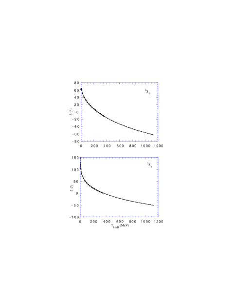
FIG. 3.: The singlet and triplet phase shifts to 1.2 GeV in lab energy for Model 1 (solid line), Model 3 (dashed line), and Model 3I (dotted line). The Nijmegen 1993 phase shift data are shown up to 350 MeV (Ref. 21) (black circles). Note that the phase shifts in both cases are nearly indistinguishable.

In the case of Models 3 and 3I there are ten parameters: six coupling constants and four form factor parameters. Unlike the case of Model 1, the singlet and triplet couplings have different restrictions placed upon them. For the singlet case, $p_{c}$ will be fixed using the location of the zero in the phase shift, as detailed above, reducing the number of parameters to nine. It was determined that $g_{11}$ needs to be a fitted parameter in this case, in order to reduce $\chi^{2}$ to its optimum value. There are, however, restrictions on several of the other coupling constants, specifically, $g_{12}=g_{13}$ and $g_{22}=g_{33}$. These four couplings are then fixed to constant values, reducing the number of parameters to five.

The choice of values for certain coupling constants may seem arbitrary. It was discovered during initial fitting trials that the fits were most sensitive to the values of the form factor parameters, and rather less sensitive to most of the tower couplings. Therefore, many of the tower couplings were fixed at historically useful values, preserving certain symmetries which seemed to consistently appear in successful fits. These values, for both the form factor parameters and the tower couplings, are given in Table I. While the fitting procedure is most sensitive to the values of the form factor parameters, it also shows some sensitivity to the values of $g_{11}$ and $g_{23}$. These parameters were therefore allowed to vary, while the other couplings were fixed such that the proportions of the couplings were maintained. For the triplet case, the full set of restrictions on $p_{c}$ and $g_{11}$ is once again applied; only $g_{12}$ and $g_{23}$ are allowed to vary. Once again, the restriction placed on the remaining coupling constants, $g_{13}=g_{22}=g_{33}$, is designed to maintain the proportions of the couplings. Thus, there are still only five free parameters in the triplet case, but they are different from those in the singlet case.

We now present numerical results for all three models discussed above, as well as our analysis of the significance of these results. First are the phase shifts, shown in Table III for the fitting region (below 350 MeV) for the three models together with the Nijmegen 1993 values. All three models give nearly indistinguishable fits to the Nijmegen phase shifts, with excellent $\chi^{2}$s. Clearly, there is no significant difference between the models as regards the phase shifts below 350 MeV. This is as expected; substantial changes in the phase shifts are not anticipated until one goes above the inelastic threshold.

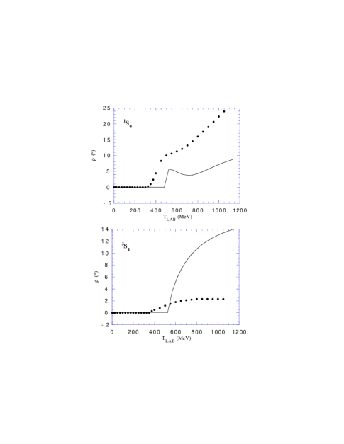
FIG. 4.: Inelasticities for Model 3I. The shape of the ${}^{1}S_{0}$ inelasticity, while more pronounced than others, is not unusual. The black dots are the inleasticities of Arndt and collaborators (Ref. 24).

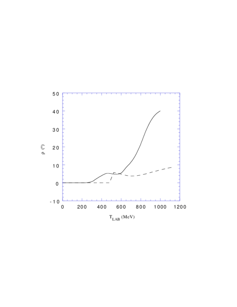
FIG. 5.: The ${}^{1}S_{0}$ inelasticities of van Faassen and Tjon (Ref. 12) (solid curve) and the Model 3I (dashed curve). Note that the shape of the Model 3I inelasticity is similar to that of van Faassen and Tjon, though more pronounced.

After the parameters are determined, the singlet and triplet phase shifts are calculated out to 1.2 GeV in lab energy and are shown in Fig. 3 (the Nijmegen 1993 phases are also shown in the fitting region). All three models fit the phase shifts extremely well. More importantly, note that the phase shifts for all three models are nearly identical in the entire range, despite the fact that the onset of inelasticity in Model 3I is at 492 MeV. The inelasticities for Model 3I are shown in Fig. 4, along with the inelasticities of Arndt and collaborators [26]. We have chosen to plot $\rho$, which is defined by $\eta=\cos\rho$. Some readers may be puzzled by the shape of the singlet inelasticity. In Fig. 5 we show the inelasticities for the ${}^{1}S_{0}$ np partial wave of van Faassen and Tjon [15] together which those of our Model 3I. Ours is more pronounced than that of van Faassen and Tjon, but the structure is similar. Some deviation in both the magnitude and shape of the inelasticity is expected since the source of inelasticity in our model arises from the production of a zero-width nucleon resonance like the Roper, instead of the more realistic coupling to a continum $\pi NN$ channel associated with the onset of production of the $\Delta$ resonance.

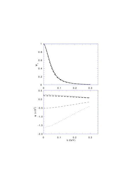
FIG. 6.: Deuteron wave functions for Model 1 (solid curves), Model 3 (dashed curves), and Model 3I (dotted curves). In the lower graph, the bold face curves are the $\psi_{2}$ components, while the normal curves are the $\psi_{3}$ components. These wave functions are dimensionless due to the manner in which they are normalized.

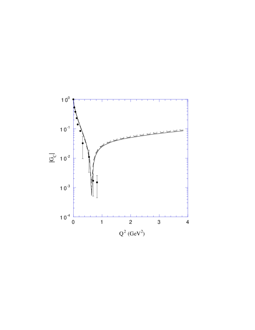
FIG. 7.: The deuteron form factor for the three models. The curves are as in Fig. 6. The black circles are data from Ref. 25.

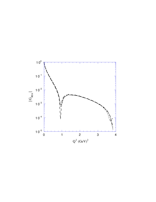
FIG. 8.: The relativistic impulse approximation contribution to the deuteron form factor. The curves are as in Fig. 7. Note the presence of an additional minimum for Model 3I.

We have also plotted the deuteron wave function for each of the three models in Fig. 6. All the wave functions are normalized in the following manner:

$$\psi_{i}(k)=\frac{\phi_{i}^{B}(k)}{\phi_{1}^{B}(0)}.$$ (6)

Clearly, the contributions from $\psi_{2}$ and $\psi_{3}$ are very small indeed.

Finally, we examine the deuteron form factor, shown in Fig. 7. Note that, in spite of the unrealistic simplicity of the models, all three of them describe the data [27] resonably well. We attribute this to the fact that each has been fitted to the ${}^{3}S_{1}$ phase shifts. There is a small gap between the three curves most prominently seen at high $Q^{2}$, where the average percent difference between Model 1 and Model 3I is 12%. This effect can only be due to the presence of the additional resonances in the three-member models. A small shift between Models 3 and 3I can also be seen.

The separation of the curves in Fig. 7, as well as the reasonable comparison to the data, appears to be due entirely to the presence of the interaction current. Fig. 8 shows the relativistic impulse approximation contributions for the three models, which we denote by $F_{I}$. We see that they are nearly identical, except for the additional minimum just visible near 4 ${\rm GeV}^{2}$ in Model 3I, and would not fit the data alone. We emphasize that only the diagonal terms of the interaction current have been included in this calculation of the deuteron form factor (recall that $\zeta_{ij}=\delta_{ij}$). Inclusion of the off-diagonal terms would likely increase the interaction current contribution, and change the final result for the deuteron form factor.

Clearly there is an effect due to the presence of the resonances in the three-member tower models, most easily seen in the calculation of the deuteron form factor, but even there it is rather small. However, the question must be asked, are the effects truly small, or are they small in this case because the inelasticities themselves are small? It is with this idea in mind that, in the next section, the effects of large inelasticity on the tower model shall be explored.

D An exploration of large inelasticity

As seen in the previous section, Model 3I has a relatively small inelasticity (but bigger that the actual data, as shown in Fig. 4), yet there seems to be an effect visible in the deuteron form factor. We now explore this effect, specifically to discover if greater inelasticity will produce larger effects in such calculated quantities. A criticism frequently leveled at current models is that the inelasticities cannot be ignored as one proceeds to larger $Q^{2}$. How large do the inelasticities need to be before one can no longer ignore their effects? It is known that in other partial waves the true $NN$ system has larger inelasticities than those found for this model, thus it seems reasonable to explore regions of large inelasticity.

In order to accomplish this, we choose to work backwards, in a sense. Rather than try to fit the known inelasticities of the $NN$ system with a tower model, we chose a simpler course of action, in keeping with a first exploration of these concepts. First, a set of data was created, based on Model 3I, with much larger inelasticity. Then, a one-member tower model, similar to Model 1, was fit to the low energy data of this new data set. The full set of calculations were then completed for both the new data and the new model. This gives us insight into the question of large inelasticity in the simplest and most direct way possible.

The large inelasticity data set was created by adjusting the Roper couplings of Model 3I, that is, $g_{12}$, $g_{22}$, and $g_{23}$, such that the inelasticity $\rho$ increased to 40-50 degrees, while maintaining the shape of the phase shifts as much as possible. The restrictions placed on the couplings in Sec. I C are also kept intact. The parameters for this set of data, called the LI data set, can be found in Table IV. This table also includes the parameters of the one tower model, referred to as Model 1LI, which was fit to this data set. The phase shifts for both the LI data set and Model 1LI are given in Table V. Note that the changes in the phase shift are very slight for the singlet case, but somewhat more pronounced in the triplet (see Table III for the Nijmegen 1993 phase shift data). Even though the $\chi^{2}$ for the triplet fit of Model 1LI seems quite large, the fit is quite good, as we will see below. The binding energy of the deuteron for both the data set and the model are given in Table VI.

TABLE IV.: Parameters in the LI data set and Model 1LI. Numbers in bold face were varied during the fitting procedure. The form factor parameters and all masses are in GeV; all the coupling constants have dimensions ${\rm GeV}^{4}$.

	LI Data Set		Model 1LI
Parameter	${}^{1}S_{0}$	${}^{3}S_{1}$	${}^{1}S_{0}$	${}^{3}S_{1}$
$\alpha$	0.197750	0.150054	0.197579	0.075051
$\beta$	1.10168	1.28994	1.10175	1.31118
$\gamma$	0.172141	0.129887	0.172310	0.058073
$p_{c}$	0.3492	0.412689	0.3492	0.412689
$g_{11}$	-1511.44	-1906.51	-1534.46	-2758.70
$g_{12}$	200.0	1000.0
$g_{13}$	200.0	-600.0
$g_{22}$	-60.0	-600.0
$g_{23}$	1700.0	800.0
$g_{33}$	-60.0	-600.0
$\chi^{2}$			0.029	31.60
$m_{1}$	0.93825		0.93825
$m_{2}$	1.17
$m_{3}$	1.52

TABLE V.: Values for the phase shifts below 350 MeV for the LI data set and Model 1LI.

$T_{{\rm LAB}}$	LI Data Set		Model 1LI
	${}^{1}S_{0}$	${}^{3}S_{1}$	${}^{1}S_{0}$	${}^{3}S_{1}$
$1.0$	$55.63$	$140.6$	$55.58$	$141.2$
$5.0$	$61.25$	$109.1$	$61.26$	$108.3$
$10.0$	$58.52$	$93.78$	$58.56$	$92.78$
$25.0$	$50.06$	$73.11$	$50.13$	$73.44$
$50.0$	$40.01$	$57.21$	$40.08$	$58.82$
$75.0$	$32.46$	$47.31$	$32.53$	$49.36$
$100.0$	$26.24$	$39.84$	$26.30$	$41.94$
$125.0$	$20.94$	$33.78$	$20.99$	$35.86$
$150.0$	$16.2$	$28.57$	$16.24$	$30.51$
$175.0$	$11.96$	$24.02$	$11.99$	$25.79$
$200.0$	$8.003$	$19.89$	$8.025$	$21.45$
$225.0$	$4.384$	$16.17$	$4.397$	$17.52$
$250.0$	$1.022$	$12.73$	$1.025$	$13.86$
$275.0$	$-2.322$	$9.559$	$-2.329$	$10.46$
$300.0$	$-5.284$	$6.62$	$-5.301$	$7.277$
$325.0$	$-8.146$	$3.86$	$-8.174$	$4.266$
$350.0$	$-10.87$	$1.284$	$-10.91$	$1.428$

The inelasticities for the data set LI are shown in Fig. 9, and the phase shifts are shown in Fig. 10. The presence of the low mass “Roper” resonance can be seen in the kink in the LI data set at about 500 MeV, which is at the onset of inelasticity. Fig. 11 shows the deuteron wave function for the LI data set and corresponding model. It is clear that the inelastic effects are much stronger than in the previous case; the $\psi_{2}$ and $\psi_{3}$ components are about ten times stronger than before.

TABLE VI.: Binding energy of the deuteron as calculated in each of the large inelastic cases. The percent error shown is the error between the calculated value and the expected value 2.22 MeV. The energies are given in MeV.

	$LIData$	$Model1LI$
$BindingEnergy$	$2.47$	$2.33$
$PercentError$	$11.3$	$5.0$

FIG. 9.: The singlet and triplet inelasticities for the LI data set.

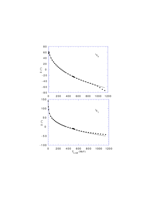
FIG. 10.: The phase shifts to 1.2 GeV for the Model 1LI (solid line) and the LI data set (black circles). Note that the kink in the triplet phase shift for the LI data set occurs exactly at the inelastic threshold.

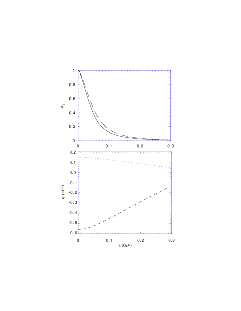
FIG. 11.: Deuteron wave functions for Model 1LI (solid curves) and LI data (broken curves). In the lower graph, the dashed line is the curve for $\psi_{30}$, while the dotted line is $\psi_{20}$. These wave functions are dimensionless due to the manner in which they are normalized.

Finally, we turn to the most noticable demonstration of the effects of the resonances: the deuteron form factor in the large inelastic case, shown in Fig. 12. Note the pronounced splitting between the model and the data, as well as the slight shift in the zero. Clearly, the resonances are finally having an effect. Our thoughts on this matter will be summarized in the next section.

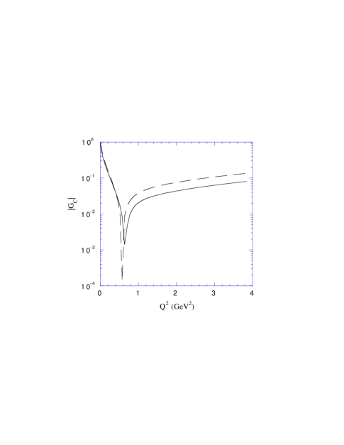
FIG. 12.: The deuteron form factor for the large inelastic model and data set. The curves are as in Fig. 11.

E Conclusions

The major conclusions of this paper are summarized as follows.

1. The low energy $NN$ data can be fit by tower models using either the proton alone (Model 1) or a tower consisting of the proton, the Roper, and the ${\rm D}_{13}$ (Models 3 and 3I). Model 1 has three parameters in both the singlet and triplet case; Models 3 and 3I have five parameters each. It has been noted that the fits do not depend strongly on the coupling constants, but rather on the three form factor parameters. Therefore, certain symmetries have been exploited in fixing several of the remaining coupling constants. In the case of Model 3I, the Roper mass is set equal to 1.17 GeV in order to ensure that some inelasticity appears within the range of interest ($T_{{\rm LAB}}=0-1.2$ GeV). Only slight effects are seen from this inelasticity on such properties of the deuteron and its wave function and form factor.

2. Three-member tower models which have small inelasticity fit the data just as well as models having no inelasticity. The differences between these models and a model with no higher order resonances are slight, and thus one might conclude that no further investigation is warranted. However, unless models with large inelasticity are explored, we cannot be sure whether the effects are small because the inelasticities themselves are small, or because inelasticity truly has no effect on the system whatsoever.

3. In order to explore the effects of large inelasticity, an adjusted data set was produced by increasing the Roper couplings in Model 3I. This large inelasticity data set was then fit below 350 MeV using a proton-only tower model. Much larger effects of the resonances are seen in this case. In this case of unrealistically large inelasticity the deuteron form factor is changed at large $Q^{2}$ by about a factor of 2, which can certainly be detected by the precision experments which will be carried out at Jefferson Lab.

In summary, our simple model suggests that the impact of nucleon resonances on the deuteron form factor will be substantial only if the inelasticity in the deuteron channel is substantial (which is not the case in the $S$-wave channel). However, we have not explored the effects of spin, the coupling to the $D$-wave channel, or the excitation of nucleon resonances by the electromagnetic current, so our conclusions can only be very preliminary. Further study is certainly warranted to assess the sizes of these additional effects.

This concludes our overview and summary of this work. The following sections will discuss the work in greater detail, beginning with the definition of the general tower of states model, and concluding with model-specific results.

II General theory

In this part the general framework of the tower of states model will be presented. The relativistic scattering equation is obtained, and an analytic solution for the $M$-matrix produced. Locations of bound state poles are also discussed. The subject of unitarity is then discussed and relations for the phase shifts obtained. Next, the inelastic scattering matrix is developed and the relations for the phase shift and the inelasticity parameter derived. Then the gauge invariance of the model is explored. Finally, we derive the expression for the deuteron form factor.

A General description of the tower of states model

We define the tower of states to be the proton and all of its charged excited states, and assume that the neutron remains unexcited by the interaction while the proton can be transformed into any of its excited states. The interaction which carries the $i$th member of this tower (and a neutron) into the $j$th member (and a neutron) is illustrated in Fig. 1 and takes the form

$${\cal V}_{ij}=g_{ij}f\left[x(p_{n}^{\prime},D)\right]f\left[x(p_{n},D)\right]\,,$$ (7)

where $x(p_{n},D)$ is defined by

$$x(p_{n},D)=p_{n}^{2}-\frac{(p_{n}\cdot D)^{2}}{D^{2}}\,,$$ (8)

with $p_{n}$ the four-momentum of the neutron and $D$ the total four-momentum. Also, $g_{ij}$ is the strong coupling between the $i$th and $j$th tower members, and $f$ is the Tabakin-style form factor defined in Eq. (2). For simplicity we will sometimes use the notation $x=x(p_{n},D)$ and $x^{\prime}=x(p_{n}^{\prime},D)$; when necessary the arguments will be written in full to avoid confusion. The variable $x$ is unchanged by the substitution $p_{n}\to p_{n}+\lambda D$, so that $x(p_{n},D)=x(p,D)$. Note also that our form factor is not equal to unity when both particles are on the mass shell, as is the case with many form factors.

It is important to remember that the neutron is placed consistently on the mass shell at all times and is not a member of the tower of states. The proton and neutron are treated as non-identical particles, which is possible if we limit ourselves to the $np$ system only (which includes the deuteron). The coupling of the photon to the neutron will be neglected in this simple, begining model. The subscript o shall be used to indicate quantities associated with the neutron, while quantities associated with the $i$th tower member, such as masses, will be given a subscript $i$. However, the four-momentum of the neutron will be labeled with $n$ to avoid confusion with the $0$th component of the vector $p$, while the tower particle four-momentum will be written without subscripts. The quantities $m_{1}=m_{o}=0.93825$ GeV will be used interchangeably. Outgoing momenta are distinguished from incoming momenta by the use of the prime, and internal momenta are generally denoted by k, without subscripts. Finally, quantities written in bold face are three-vectors.

B Analytic solution for the $M$-matrix and bound state wave functions

We would like to find an analytic form for the scattering matrix [22], to simplify the calculation of phase shifts and other such important quantities. Begin with the most general form for a two-body scattering equation

$$M(p,p^{\prime};D)={\cal V}(p,p^{\prime};D)+\int_{k}{\cal V}(p,k;D)G(k,D)M(k,p^{\prime};D)\,,$$ (9)

where M is the scattering amplitude, ${\cal V}$ is the kernel, $\int_{k}$ represents an integration over the unspecified internal four-momentum, and G is the two-body propagator. The exact forms of these terms will be discussed in Sec. III.

Assuming that the kernel is sufficiently small, perturbation theory permits us to obtain an iterative solution to the above equation. This solution takes the form

$$M={\cal V}+\int{\cal V}G{\cal V}+\int\int{\cal V}G{\cal V}G{\cal V}+\cdots+\left(\int{\cal V}G\right)^{n}{\cal V}+\cdots\,,$$ (10)

also shown diagrammatically in Fig. 13. This may be recognized as a geometric series, which has a simple analytic form,

$$M=\left(1-\int{\cal V}G\right)^{-1}{\cal V}\,.$$ (11)

Note that because of the form of the kernel, each term in the sum (10) will contain a factor of $f(x^{\prime})f(x)$, one form factor each for the incoming and outgoing tower member. It therefore becomes convenient to define the reduced $M$-matrix ${\cal M}$, such that its elements are defined by $M_{ij}=f(x^{\prime})f(x){\cal M}_{ij}$.

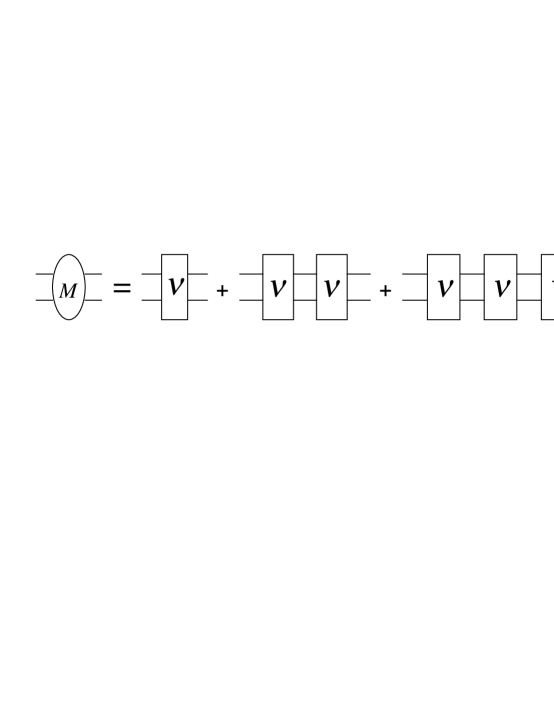
FIG. 13.: Diagrammatic form of Eq. (2.4).

In terms of matrices, Eq. (11) can be written

$${\cal M}=(1-g{\cal G})^{-1}g\,,$$ (12)

where the matrix ${\cal G}$ is a diagonal matrix of propagators with elements

$${\cal G}_{\ell}=\int_{k}f^{2}(k)G_{\ell}\,,$$ (13)

and $g$ is the matrix of the strong coupling constants $\{g_{ij}\}$ defined in Sec. II A and $G_{\ell}$ is the propagator for the $\ell$th tower member.

To locate the bound state poles (if any) of Eq. (11) introduce the matrix $A=(1-g{\cal G})$ and write the solution (12) as

$${\cal M}=\frac{C^{\rm T}g}{\det A}\,,$$ (14)

where $C$ is the cofactor matrix of A. The full matrix $M$ is then

$$M=f(x^{\prime})\frac{C^{\rm T}g}{\det A}f(x)\,.$$ (15)

Written in this form it is clear that the locations of any bound state poles can be found simply by solving the equation $\det A=0$.

To find the bound state wave function, recall that the integral equation for the bound state is

$$\Gamma(p,D)=\int_{k}{\cal V}(p,k;D)G(k,D)\Gamma(k,D)\,,$$ (16)

where $\Gamma$ is the bound state vertex function. This equation can also be written in matrix notation

$$(1-{\cal VG})\Gamma=0\,.$$ (17)

Since the interaction is separable, the solution to this equation is

$$\Gamma(p,D)=\left(\begin{array}[]{c}c_{1}\\ c_{2}\\ \vdots\\ \end{array}\right)f(x)$$ (18)

for as many tower members as we choose. The bound state wave function is

$$\phi={\cal N}G\Gamma,$$ (19)

where ${\cal N}$ is a normalization constant and $G$ is the diagonal matrix of propagators with elements $G_{\ell}$. Therefore the solution of Eq. (17) determines the wave function up to a normalization constant.

C Unitarity

The most general unitarity relation, derivable from Eq. (9) [22], is

$$M-\bar{M}= \int_{k}\bar{M}(G-\bar{G})M$$ (20)

$$= M^{\ast}({\cal G}-{\cal G}^{\ast})M\,,$$ (21)

where the last is the matrix version of the unitary relation. Note that the bars may be changed to complex conjugates since there is no Dirac structure in the problem, and hence the equation reduces to the following conditions on the matrix elements of $M$

$$2i\,{\rm Im}M_{ij}=M_{i\ell}^{\ast}({\cal G}_{\ell}-{\cal G}_{\ell}^{\ast})M_{\ell j}\,,$$ (22)

where the implied summation over $\ell$ runs over all members of the tower.

If we are below the production threshold for any tower member except the proton,

$$\rho_{\ell}=\frac{{\cal G}_{\ell}-{\cal G}_{\ell}^{\ast}}{2i}=0\quad\ell>1\,.$$ (23)

This allows us to simplify Eq. (22) to

$${\rm Im}M_{ij}=\rho_{1}M_{i1}^{\ast}M_{1j}.$$ (24)

For determining the phase shifts, only the expression for $M_{11}$ need be considered, and

$${\rm Im}M_{11}=\rho_{1}|M_{11}|^{2}\,,$$ (25)

where $\rho_{1}$ is the relativisitic phase space factor

$$\rho_{1}=\frac{\sqrt{W^{2}-4m_{o}^{2}}}{8\pi W}\,.$$ (26)

Note the similarity between Eq. (25) and the unitarity relation for the $\ell$th partial wave in nonrelativistic scattering

$${\rm Im}f_{\ell}=\frac{p}{K}|f_{\ell}|^{2},$$ (27)

where K is a constant, usually equal to unity in nonrelativistic theory. Therefore, the standard identifications may be made,

$$f_{\ell} \leftrightarrow -M_{11}$$ (28)

$$\frac{p}{K} \leftrightarrow \rho_{1}\,,$$ (29)

(where the minus sign in the first relation comes from a comparison of the integral equations and not the unitary relation) allowing us to write

$$M_{11}=-\frac{e^{i\delta_{1}}\sin\delta_{1}}{\rho_{1}}\,,$$ (30)

which implies

$${\rm Re}M_{11} = -\frac{\cos\delta_{1}\sin\delta_{1}}{\rho_{1}}$$ (31)

$${\rm Im}M_{11} = -\frac{\sin^{2}\delta_{1}}{\rho_{1}}\,.$$ (32)

These can be combined to yield a single expression for $\delta_{1}$,

$$\delta_{1}=\arctan\left(\frac{{\rm Im}M_{11}}{{\rm Re}M_{11}}\right).$$ (33)

This is the general expression for the elastic phase shift. In order to fit to the phase shift data, the real and imaginary parts of $M_{11}$ must be written in terms of the free parameters. This will be discussed in Sec. III.

D Inelasticity

To explore the inelastic scattering region for the tower model [28] we generalize the structure of the scattering matrix to include the possibility of inelasticity:

$$-M_{11}=\frac{\eta e^{2i\delta_{1}}-1}{2i\rho_{1}},$$ (34)

where $\eta=\cos\rho<1$ is the inelasticity parameter. Note that elastic scattering corresponds to $\eta=1$ (or $\rho=0$), and that as $\eta$ decreases toward zero (or $\rho$ toward $\pi/2$) the scattering becomes increasingly inelastic.

It follows from (34) that the real and imaginary parts of $M_{11}$ are now

$${\rm Im}M_{I} = \frac{1}{\rho_{1}}(\eta\cos 2\delta_{1}-1)$$ (35)

$${\rm Re}M_{I} = -\frac{1}{\rho_{1}}\eta\sin 2\delta_{1}\,.$$ (36)

Solving for the two unknowns, $\eta$ and $\delta_{1}$, gives

$$\eta = \frac{\rho_{1}{\rm Im}M_{11}+1}{\cos 2\delta_{1}}$$ (37)

$$\tan 2\delta_{1} = -\frac{{\rm Re}M_{11}}{{\rm Im}M_{11}+{\displaystyle\frac{1}{\rho_{1}}}}\,.$$ (38)

We will return to these expressions for the phase shift and inelasticity parameter in Sec. III.

E Electromagnetic current and gauge invariance

In this section we describe the one and two body currents, and show that the model is exactly gauge invariant.

Charge conservation requires that the coupling between the photon and a given tower member be of the form $e_{ij}=\zeta_{ij}e$, where e is the electromagnetic charge of the proton and $\zeta_{ij}$ is a scaling factor which must equal unity if $i=j$. The off-diagonal terms are not constrained by charge conservation, but the simplest way to insure that the model is gauge invarinat is to require them to be be transverse, that is, $q_{\mu}j^{\mu}=0$. Finally, we require that the diagonal component of the current satisfy a Ward-Takahashi identity [29],[30], which may be expressed in a compact fashion,

$$q_{\mu}j^{\mu}_{ij}(p^{\prime},p)=-e\left[G_{i}^{-1}\left(p^{\prime 2}\right)-G_{j}^{-1}\left(p^{2}\right)\right]\delta_{ij}\,,$$ (39)

where $p$ and $p^{\prime}$ are the initial and final momentum of the tower member, respectively. This restriction is satisfied by the following form of the electromagnetic current of the tower member:

$$j_{ij}^{\mu}(p^{\prime},p)=e_{ij}F_{ij}(Q^{2})\left(P^{\mu}-\frac{P\cdot q}{q^{2}}q^{\mu}\right)+e_{ij}\delta_{ij}\left(\frac{P\cdot q}{q^{2}}q^{\mu}\right)\,,$$ (40)

where $P=p^{\prime}+p$ and the form factors $F_{ij}(Q^{2})$ represent the structure of the current due to the true (nonpointlike) nature of the tower members. To avoid kinematic singularities we require

$$F_{ii}(0)= 1$$ (41)

$$F_{ij}(0)= 0\,.$$ (42)

Except for these requirements, the form factors need not be further specified at this time.

Because the strong form factors $f$ depend on the total four-momentum, we expect them to generate an interaction current. Using a technique similar to that of Ito, Buck and Gross [25], and assuming that $\zeta_{ij}=\delta_{ij}$ for simplicity, leads to the following interaction current (see the Appendix for details)

$$j_{ij}^{\mu^{INT}}(p_{n}^{\prime},p_{n};D^{\prime},D)=eg_{ij}\Biggl{\{} {\cal Z}^{\prime\mu}\frac{f\left[x(p_{n}^{\prime},D^{\prime})\right]-f\left[x(p_{n}^{\prime},D)\right]}{x(p_{n}^{\prime},D^{\prime})-x(p_{n}^{\prime},D)}f\left[x(p_{n},D)\right]$$ (44)

$$+{\cal Z}^{\mu}f\left[x(p_{n}^{\prime},D^{\prime})\right]\frac{f\left[x(p_{n},D^{\prime})\right]-f\left[x(p_{n},D)\right]}{x(p_{n},D^{\prime})-x(p_{n},D)}\Biggr{\}}\,,$$

where

$${\cal Z}^{\mu}=\frac{1}{2D^{2}D^{\prime 2}}\biggl{\{} (D+D^{\prime})^{\mu}\left[(p_{n}\cdot D)^{2}+(p_{n}\cdot D^{\prime})^{2}\right]$$ (46)

$$-p_{n}^{\mu}\;\;\;\;p_{n}\cdot\!(D+D^{\prime})\left(D^{2}+D^{\prime 2}\right)\biggr{\}}\,,$$

and ${\cal Z}^{\prime\mu}$ is obtained from ${\cal Z}^{\mu}$ by replacing $p_{n}$ by $p^{\prime}_{n}$. Contracting $q_{\mu}$ into this current gives

$$q_{\mu}j_{ij}^{\mu^{INT}}(p_{n}^{\prime},p_{n};D^{\prime},D)=e\biggl{\{}{\cal V}_{ij}(p_{n}^{\prime},p_{n};D^{\prime})-{\cal V}_{ij}(p_{n}^{\prime},p_{n};D)\biggr{\}}\,.$$ (47)

Recalling that the bound state is generated by the infinte sum given in Eq. (10), it can be shown that the electrodisintegration process is described by the four diagrams shown in Fig. 14. We will show that these diagrams, together with the conditions (39) and (47), are sufficient to ensure that the electrodisintegration process is gauge invariant.

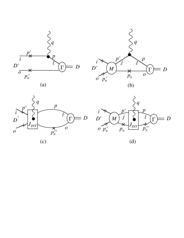
FIG. 14.: The four diagrams required for the calculation of the electrodisintegration process. The large boxes with photons coupling to them are interaction currents, the oval with a $\Gamma$ is a bound state vertex, and the circle with an $M$ is a scattering matrix.

Note first that all four diagrams have the same incoming state, namely

$$\phi_{\ell}^{i}=\phi_{\ell}^{B}(p_{n},D)=G_{\ell}(p)\Gamma_{\ell}(p_{n},D),$$ (48)

where $\phi_{\ell}^{B}$ is the bound state wave function of a neutron and the $\ell$th member of the tower of states. The final states, however, are different. For diagrams 14(a) and 14(c) there is no final state interaction and the final state is a plane wave state with

$$\bar{\phi}_{ij\;{\rm pw}}^{f}(p^{\prime}_{n},p_{n};D^{\prime})=2E\,\delta_{ij}\,(2\pi)^{3}\delta^{3}(p^{\prime}_{n}-p_{n})\,,$$ (49)

where $E=\sqrt{m_{n}^{2}+p_{n}^{2}}$. Diagrams 14(b) and 14(d) include the final state interactions. In the notation of the figures, this is

$$\bar{\phi}_{ij\;{\rm scatt}}^{f}(p^{\prime}_{n},p_{n};D^{\prime})=\bar{M}_{ij}(p_{n}^{\prime},p_{n};D^{\prime})G_{j}(p^{\prime}).$$ (50)

These two processes can be combined by introducing the total final state wave function

$$\bar{\phi}_{ij}^{f}(p^{\prime}_{n},p_{n};D^{\prime}) = \bar{\phi}_{ij\;{\rm pw}}^{f}(p^{\prime}_{n},p_{n};D^{\prime})+\bar{\phi}_{ij\;{\rm scatt}}^{f}(p^{\prime}_{n},p_{n};D^{\prime})$$ (51)

$$= \bar{M}_{ij}(p_{n}^{\prime},p_{n};D^{\prime})G_{j}(p^{\prime})+2E\,\delta_{ij}\,(2\pi)^{3}\delta^{3}(p_{n}^{\prime}-p_{n})\,.$$ (52)

Using this notation, the four diagrams shown in Fig. 14 can be written

$$\langle J^{\mu}\rangle_{i}= \int{d^{3}p_{n}\over(2\pi)^{3}2E}\;\bar{\phi}_{ij}^{f}(p^{\prime}_{n},p_{n};D^{\prime})j_{j\ell}^{\mu}(p^{\prime},p)\phi_{\ell}^{B}(p_{n},D)$$ (54)

$$+\int\frac{d^{3}p_{n}\;d^{3}p^{\prime\prime}_{n}}{(2\pi)^{6}4EE^{\prime\prime}}\,\bar{\phi}_{ij}^{f}(p^{\prime}_{n},p_{n};D^{\prime})\,j_{j\ell}^{\mu^{INT}}(p,p^{\prime\prime};D^{\prime},D)\,\phi_{\ell}^{B}(p^{\prime\prime}_{n},D)\,,$$

where summation over repeated indicies is implied.

Now, to demonstrate that the current (54) is gauge invariant we contract it with $q_{\mu}$ and use the relations (39) and (47) to obtain

$$q_{\mu}\langle J^{\mu}\rangle_{i}= -e\int{d^{3}p_{n}\over(2\pi)^{3}2E}\bar{\phi}_{ij}^{f}(p^{\prime}_{n},p_{n};D^{\prime})\left\{G_{j}^{-1}\left(p^{\prime}\right)-G_{j}^{-1}(p)\right\}\phi_{j}^{B}(p_{n},D)$$ (57)

$$+e\int\frac{d^{3}p_{n}\;d^{3}p^{\prime\prime}_{n}}{\left(2\pi\right)^{6}4EE^{\prime\prime}}\;\bar{\phi}_{ij}^{f}(p^{\prime}_{n},p_{n};D^{\prime})$$

$$\quad\times\biggl{\{}{\cal V}_{j\ell}(p_{n},p_{n}^{\prime\prime};D^{\prime})-{\cal V}_{j\ell}(p_{n},p_{n}^{\prime\prime};D)\biggr{\}}\phi_{\ell}^{B}(p^{\prime\prime}_{n},D)\,.$$

We can reduce the expressions $G_{j}^{-1}(p)\phi_{j}^{B}$ and $\bar{\phi}_{ij}^{f}G_{j}^{-1}(p^{\prime})$ which occur in the first term of Eq. (57) by using the fact that $\bar{\phi}_{ij}^{f}$ and $\phi_{j}^{B}$ satisfy the spectator equation:

$$G_{j}^{-1}(p)\phi_{j}^{B}(p_{n},D)=\int\frac{d^{3}p^{\prime\prime}_{n}}{(2\pi)^{3}2E^{\prime\prime}}{{\cal V}}_{jm}(p_{n},p_{n}^{\prime\prime};D)\phi_{m}^{B}(p^{\prime\prime}_{n},D)\,,$$ (58)

and similiarly for the final state. Using these equations to rewrite the first term of Eq. (57) yields

$$q_{\mu}\langle J^{\mu}\rangle_{i}= -e\int\frac{d^{3}p_{n}\;d^{3}p^{\prime\prime}_{n}}{\left(2\pi\right)^{6}4EE^{\prime\prime}}\biggl{\{}\bar{\phi}_{im}^{f}(p^{\prime}_{n},p^{\prime\prime}_{n};D^{\prime}){\cal V}_{mj}\left(p^{\prime\prime}_{n},p_{n};D^{\prime}\right)\phi_{j}^{B}(p_{n},D)$$ (62)

$$\qquad\qquad\qquad\qquad-\bar{\phi}_{ij}^{f}(p^{\prime}_{n},p_{n};D^{\prime}){{\cal V}}_{jm}\left(p_{n},p^{\prime\prime}_{n};D\right)\phi_{m}^{B}(p^{\prime\prime}_{n},D)\biggr{\}}$$

$$+e\int\frac{d^{3}p_{n}\;d^{3}p^{\prime\prime}_{n}}{\left(2\pi\right)^{6}4EE^{\prime\prime}}\;\bar{\phi}_{ij}^{f}(p^{\prime}_{n},p_{n};D^{\prime})$$

$$\quad\times\biggl{\{}{\cal V}_{j\ell}(p_{n},p_{n}^{\prime\prime};D^{\prime})-{\cal V}_{j\ell}(p_{n},p_{n}^{\prime\prime};D)\biggr{\}}\phi_{\ell}^{B}(p^{\prime\prime}_{n},D)$$

$$= 0\,,$$ (63)

where the cancellation follows from interchanging the $p_{n}$ and $p^{\prime\prime}_{n}$ integrations in the first term and relabeling the sums. This completes our proof that the current is gauge invariant.

F Deuteron form factor

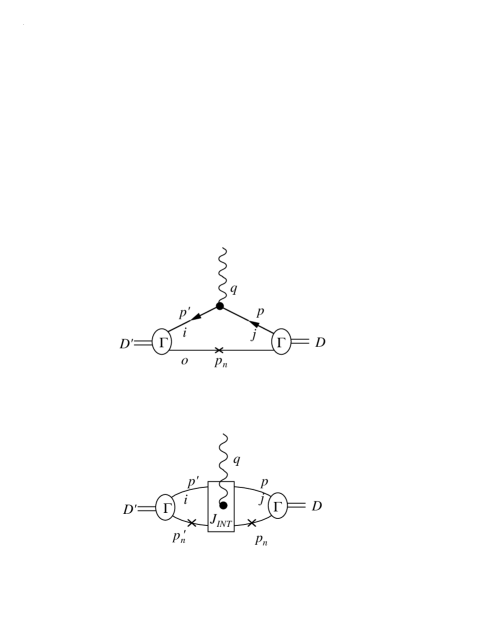
FIG. 15.: The diagrams needed to calculate the deuteron form factor. Diagram (a) is the relativistic impulse approximation and diagram (b) includes the interaction current.

In this section we discuss the calculation of the deuteron current given by the two diagrams shown in Fig. 15. The deuteron form factor, $G_{C}$, is defined by the relation

$$J_{p}^{\mu}=e\,G_{C}(Q^{2})\,(D+D^{\prime})^{\mu}\,.$$ (64)

The form factor describes the structure of the deuteron; the current for a structureless point particle is obtained from this equation by replacing $G_{C}\to 1$.

The current for the processes shown in Fig. 15 is

$$J_{D}^{\mu}= \int\frac{d^{3}p_{n}}{(2\pi)^{3}2E}\;\bar{\phi}_{i}^{B}(p_{n},D^{\prime})j_{ij}^{\mu}(p^{\prime},p)\phi_{j}^{B}(p_{n},D)$$ (66)

$$+\int\frac{d^{3}p_{n}^{\prime}\,d^{3}p_{n}}{(2\pi)^{6}4EE^{\prime}}\;\bar{\phi}_{i}^{B}(p^{\prime}_{n},D^{\prime})j^{\mu^{INT}}_{ij}(p_{n}^{\prime},p_{n};D^{\prime},D)\phi_{j}^{B}(p_{n},D)\,,$$

where the one-body and interaction currents are the same as those given in Eqs. (40) and (44). When the polarization vectors $\epsilon_{\mu}$ of the photon (including the longitudinal polarization vector associated with a virtual photon) are contracted into these currents, any terms containing $q^{\mu}$ will vanish. Using the notation shown in the relativistic impulse approximation (RIA) diagram given in Fig. 15 leads to the replacement $P^{\mu}=(D+D^{\prime})^{\mu}-2p_{n}^{\mu}$, and the effective one-body current is simply

$$j_{ij}^{\mu}=eF(Q^{2})\biggl{\{}(D+D^{\prime})^{\mu}-2p_{n}^{\mu}\biggr{\}}\,\delta_{ij}\,.$$ (67)

Since the interaction current does not contain any factors of $q_{\mu}$, it remains as given in Eq. (44).

We now extract an explicit formula for the deuteron form factor from Eq. (66). First, note that the integrand of the integral

$$I_{1}=\int\frac{d^{3}p_{n}}{(2\pi)^{3}2E}\;\bar{\phi}_{i}^{B}(p_{n},D^{\prime})\;\phi_{i}^{B}(p_{n},D)\,,$$ (68)

is an even function of the three vector ${\bf p}_{n}$ in the Breit frame, and hence in this frame

$$I^{\mu}_{p}= \int\frac{d^{3}p_{n}}{(2\pi)^{3}2E}\;\bar{\phi}_{i}^{B}(p_{n},D^{\prime})\;p_{n}^{\mu}\;\phi_{i}^{B}(p_{n},D)$$ (69)

$$= (D^{\prime}+D)^{\mu}\int\frac{d^{3}p_{n}}{(2\pi)^{3}2E}\;\bar{\phi}_{i}^{B}(p_{n},D^{\prime})\;\left[\frac{p_{n}\cdot(D+D^{\prime})}{(D+D^{\prime})^{2}}\right]\;\phi_{i}^{B}(p_{n},D)\,.$$ (70)

Since both sides of this equation are covariant, this expression holds in any frame.

The interaction current term can also be simplified in the same way. Since the initial and final states are identical, the integrand of the interaction integral is symmetric under the interchange ${\bf p}_{n}\leftrightarrow-{\bf p}^{\prime}_{n}$ in the Breit frame [which transforms $x(p^{\prime}_{n},D^{\prime})$ into $x(p_{n},D)$ and $x(p^{\prime}_{n},D)$ into $x(p_{n},D^{\prime})$], except for the terms in ${\cal Z}^{\mu}$ and ${\cal Z}^{\prime\mu}$ which are linear in the three-vector parts of $p_{n}^{\mu}$ and $p^{\prime\mu}_{n}$. These terms are odd under this interchange, and thus vanish, leaving only the time components of $p_{n}^{\mu}$ and $p^{\prime\mu}_{n}$. The interaction current can therefore be written as the product of two integrals

$$J_{D\,{\rm INT}}^{\mu}=2eg_{ij}\; \int\frac{d^{3}p^{\prime}_{n}}{(2\pi)^{3}2E^{\prime}}\;{\phi}_{i}^{B}(p^{\prime}_{n},D^{\prime})f\left[x(p_{n}^{\prime},D^{\prime})\right]$$ (71)

$$\times \int\frac{d^{3}p_{n}}{(2\pi)^{3}2E}\phi_{j}^{B}(p_{n},D){\cal Z}^{\mu}\left(\frac{f\left[x(p_{n},D^{\prime})\right]-f\left[x(p_{n},D)\right]}{x(p_{n},D^{\prime})-x(p_{n},D)}\right)\,,$$ (72)

where, for the deuteron form factor with $D^{2}=D^{\prime 2}=M_{d}^{2}$, ${\cal Z}^{\mu}$ simplifies to

$${\cal Z}^{\mu}= (D+D^{\prime})^{\mu}\;\overline{{\cal Z}}$$ (73)

$$= (D+D^{\prime})^{\mu}\;\left\{{(p_{n}\cdot D)^{2}+(p_{n}\cdot D^{\prime})^{2}\over 2M_{d}^{4}}-{\left[p_{n}\cdot(D+D^{\prime})\right]^{2}\over M_{d}^{2}\,(D^{\prime}+D)^{2}}\right\}\,.$$ (74)

Each of the two integrals in (72) is covariant, and therefore can be evaluated in any frame. The first of these two integrals depends on $D^{\prime}$ only, and is therefore a constant (which is obvious when it is evaluated in the rest frame of the outgoing deuteron). Denoting this constant by $C_{i}$

$$C_{i}=\int\frac{d^{3}p^{\prime}_{n}}{(2\pi)^{3}2E^{\prime}}\;{\phi}_{i}^{B}(p^{\prime}_{n},D^{\prime})f\left[x(p_{n}^{\prime},D^{\prime})\right]\,,$$ (75)

and using (70) and (72) gives the following result for the deuteron form factor

$$G_{C}(Q^{2})= F(Q^{2})\int\frac{d^{3}p_{n}}{(2\pi)^{3}2E}\;\bar{\phi}_{i}^{B}(p_{n},D^{\prime})\;\left[1-\frac{2p_{n}\cdot(D+D^{\prime})}{(D+D^{\prime})^{2}}\right]\;\phi_{i}^{B}(p_{n},D)$$ (77)

$$+2g_{ij}\;C_{i}\int\frac{d^{3}p_{n}}{(2\pi)^{3}2E}\phi_{j}^{B}(p_{n},D)\overline{{\cal Z}}\left(\frac{f\left[x(p_{n},D^{\prime})\right]-f\left[x(p_{n},D)\right]}{x(p_{n},D^{\prime})-x(p_{n},D)}\right)\,.$$

Note that the only the first term (the RIA) depends on the nucleon form factor, $F(Q^{2})$. The second, exchange term, is independent of this factor and depends only on the strong form factor $f$. As we will discuss in the next section, this term actually goes to a constant as $Q^{2}\to\infty$.

This concludes the discussion of the general theory of the tower of states. In the next section we will apply this to the specific models under consideration.

III Tower of States Models

In this section the detailed form of the equations appropriate for a three-member tower are presented. Then the details of the equations needed to calculate the phase shifts and inelasticity parameter for a three-member tower above the inelastic threshold of the second tower member are presented. In the final subsection the behavior of the interaction current contribution to the deuteron form factor is more carefully examined.

A Specific structure for a three-member tower

Using the spectator formalism, the generic integrals in Sec. II B become

$$\int_{k}=-\int\frac{d^{3}k}{(2\pi)^{3}2E}\,,$$ (78)

where $E=\sqrt{m_{n}^{2}+k^{2}}$ (where $k^{2}$ is the square of the three-momenta in these formulae, not to be confused with the four-momenta), and the elements of the propagator matrix (13) in the rest frame of the $NN$ system, where $D=(W,{\bf 0})$, are

$${\cal G}_{i}=-\int\frac{d^{3}k}{(2\pi)^{3}2E}\;\frac{f^{2}[x(k,D)]}{E_{i}^{2}-(W-E)^{2}}\,.$$ (79)

The momenta are labeled in Fig. 16. Here $E_{i}=\sqrt{m_{i}^{2}+k^{2}}$ and, in the rest frame,

$$f\left[x(k,D)\right]=\frac{(\alpha^{2}+{k}^{2})(p_{c}^{2}-{k}^{2})}{(\gamma^{2}+{k}^{2})(\beta^{2}+{k}^{2})^{2}}\equiv f(k^{2})\,.$$ (80)

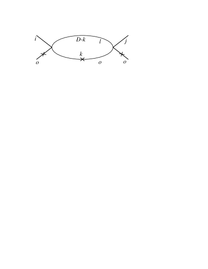
FIG. 16.: The definition of the momenta for the bubble diagram. It is these momenta which must be used in the integrals ${\cal G}_{i}$.

If $W<m_{o}+m_{i}$ (where $m_{o}=m_{n}$ as discussed above), the integrand of Eq. (79) is real for all $k$ and the integral is real. When $W>m_{o}+m_{i}$ the integrand has a pole in the range of integration located at ${k}={k}_{p}^{i}$, where

$${k}^{i}_{p}=\sqrt{\left(\frac{W^{2}-m_{i}^{2}+m_{o}^{2}}{2W}\right)^{2}-m_{o}^{2}}\,,$$ (81)

This pole gives the integral an imaginary part. The threshold for the onset of this complex behavior, in terms of the kinetic energy of the nucleon in the $NN$ laboratory system, is

$$T_{{\rm LAB}}^{i}={(m_{o}+m_{i})^{2}-4m_{o}^{2}\over 2m_{o}}\,.$$ (82)

These thresholds are given in Table VII for each of the channels discussed in Sec. I.

TABLE VII.: Thresholds for the onset of inelasticity for the various channels.

channel mass	$T_{{\rm LAB}}^{i}$
in GeV	in MeV
0.93825	0
1.17	492
1.44	1138
1.52	1344

For energies in the fitting region ($T_{{\rm LAB}}<$ 350 MeV) only ${\cal G}_{1}$ will have an imaginary part. (The case where more than one of the integrals has an imaginary part will be discussed in Sec. III B.) For all energies ${\cal G}_{1}$ can be written

$${\cal G}_{1}={\cal P}\int_{0}^{\infty}{k^{2}dk\over E}\,\frac{f^{2}(k^{2})}{W(2E-W)}+i\,{\rm Im}{\cal G}_{1}\,,$$ (83)

where ${\cal P}$ denotes the Cauchy Principle Value of the integral, and the imaginary part is

$${\rm Im}{\cal G}_{1}=\pi\,\frac{\sqrt{W^{2}-4m_{o}^{2}}}{4W}\;f^{2}(k^{2}_{1p})\,.$$ (84)

The real part can be evaluated numerically.

Now return to Eq. (15) and evaluate the $NN$ scattering amplitude, which in the tower notation is $M_{11}$. At energies below the production threshold for either of the resonances, the imaginary part of $M_{11}$ can come only from ${\cal G}_{1}$, which contributes only to the denominator $\det(1-g{\cal G})=\det A$, and recalling that the cofactor matrix of $A$ is denoted by $C$, we obtain

$$M_{11}=\frac{(C^{\rm T}\,g)_{11}}{{\rm Re}(\det A)+i{\rm Im}(\det A)}\,f(x^{\prime})f(x)\,.$$ (85)

Rationalizing the denominator gives the real and imaginary parts of $M_{11}$, and hence the phase shift in the elastic scattering region depends only on the $\det A$

$$\tan\delta_{1}=-\frac{{\rm Im}(\det A)}{{\rm Re}(\det A)}\,.$$ (86)

For a three member tower, the real and imaginary parts of $\det A$ are

$${\rm Im}(\det A) = -\left[g_{11}-(g_{11}g_{33}-g_{13}^{2}){\cal G}_{3}-(g_{11}g_{22}-g_{12}^{2}){\cal G}_{2}+B_{g}{\cal G}_{2}{\cal G}_{3}\right]{\rm Im}{\cal G}_{1}$$ (87)

$${\rm Re}(\det A) = 1-g_{33}{\cal G}_{3}-g_{22}{\cal G}_{2}+(g_{22}g_{33}-g_{23}^{2}){\cal G}_{2}{\cal G}_{3}$$ (89)

$$-\left[g_{11}-(g_{11}g_{33}-g_{13}^{2}){\cal G}_{3}-(g_{11}g_{22}-g_{12}^{2}){\cal G}_{2}+B_{g}{\cal G}_{2}{\cal G}_{3}\right]{\rm Re}{\cal G}_{1}\,,$$

where $B_{g}$ is

$$B_{g}=(g_{11}g_{22}g_{33}-g_{11}g_{23}^{2}-g_{12}^{2}g_{33}+2g_{13}g_{12}g_{23}-g_{13}^{2}g_{22})\,.$$ (90)

The deuteron vertex function for a three-member tower,

$$\Gamma=\left(\begin{array}[]{c}c_{1}\\ c_{2}\\ c_{3}\\ \end{array}\right)f(k^{2})\,,$$ (91)

is obtained from Eq. (17). The solution for $c_{2}$ and $c_{3}$ in terms of $c_{1}$ (which must be determined by normalization) is

$$c_{2} = \frac{g_{12}(1-g_{33}{\cal G}_{3})+g_{13}g_{23}}{(1-g_{22}{\cal G}_{2})(1-g_{33}{\cal G}_{3})-g_{23}^{2}{\cal G}_{2}}\;{\cal G}_{1}c_{1}$$ (92)

$$c_{3} = \frac{g_{13}(1-g_{22}{\cal G}_{2})+g_{12}g_{23}}{(1-g_{22}{\cal G}_{2})(1-g_{33}{\cal G}_{3})-g_{23}^{2}{\cal G}_{2}}\;{\cal G}_{1}c_{1}\,,$$ (93)

where the integrals ${\cal G}_{i}$ must be evaluated at $W=M_{D}$. Normalizing the wave function to unity at $k=0$, the general expression for the deuteron wave function for a three-member tower is

$$\psi_{i}(k)=\frac{\phi_{i}^{B}({k})}{\phi_{1}^{B}(0)}=\frac{c_{i}M_{D}(2m_{o}-M_{D})}{c_{1}\left(m_{i}^{2}-m_{o}^{2}+2M_{D}\sqrt{m_{o}^{2}+{k}^{2}}-M_{D}^{2}\right)}\;{\gamma^{2}\beta^{4}\over\alpha^{2}p_{c}^{2}}f(k^{2})\,.$$ (94)

Finally, we evaluate the deuteron form factor in the case of the three-member tower. The integrations in Eq. (77) are easily carried out if the momenta in Fig. 15 are evaluated in the Breit frame, where

$$p = D-p_{n}$$ (95)

$$p^{\prime} = D^{\prime}-p_{n}^{\prime}$$ (96)

$$q = (0,{\bf q})$$ (97)

$$D = \left(D_{0},-{\textstyle\frac{1}{2}}{\bf q}\right)$$ (98)

$$D^{\prime} = \left(D_{0},{\textstyle\frac{1}{2}}{\bf q}\right)\,,$$ (99)

with $D_{0}=\sqrt{M_{D}^{2}+{\bf q}^{2}/{4}}$. We use the standard notation $Q^{2}=-q^{2}={\bf q}^{2}$. For the nucleon form factor, $F(Q^{2})$, we use the dipole approximation,

$$F(Q^{2})=\left(\frac{1}{1+0.71Q^{2}}\right)^{2}\,.$$ (100)

where $Q^{2}$ is in GeV².

In the next subsection we extend the results for $M_{11}$ to the inelastic region.

B Inelasticities in the three-member tower

Since one of the tower models (Model 3I) has a significant inelastic region, in this subsection we develop the relations needed to calculate the phase shifts and inelasticities above the production threshold for particle 2.

In Section III A, the determination of the real and imaginary parts of $M$ was considerably simplified by realizing that only terms containing ${\cal G}_{1}$ could contribute to the imaginary part. In the inelastic region ${\cal G}_{2}$ will also have an imaginary part. Breaking the numerator and the denominator of Eq. (85) into their real and imaginary parts and rationalizing the denominator gives

$${\rm Im}M_{11} = \frac{{\rm Im}(C^{\rm T}g)_{11}{\rm Re}({\det A})-{\rm Re}(Cg)_{11}{\rm Im}({\det A})}{\left[{\rm Re}(\det A)\right]^{2}+\left[{\rm Im}({\det A})\right]^{2}}f(x^{\prime})f(x)$$ (101)

$${\rm Re}M_{11} = \frac{{\rm Re}(Cg)_{11}{\rm Re}({\det A})+{\rm Im}(Cg)_{11}{\rm Im}({\det A})}{\left[{\rm Re}(\det A)\right]^{2}+\left[{\rm Im}({\det A})\right]^{2}}f(x^{\prime})f(x)\,,$$ (102)

where

$${\rm Re}(C^{\rm T}g)_{11} = g_{11}(1-g_{33}{\cal G}_{3})+g_{13}^{2}{\cal G}_{3}-D{\rm Re}{\cal G}_{2}$$ (103)

$${\rm Im}(C^{\rm T}g)_{11} = -D{\rm Im}{\cal G}_{2}$$ (104)

$${\rm Re}(\det A) = 1-g_{33}{\cal G}_{3}-g_{11}{\rm Re}{\cal G}_{1}-g_{22}{\rm Re}{\cal G}_{2}$$ (108)

$$+(g_{11}g_{33}-g_{13}^{2}){\cal G}_{3}{\rm Re}{\cal G}_{1}+(g_{22}g_{33}-g_{23}^{2}){\cal G}_{3}{\rm Re}{\cal G}_{2}$$

$$+(g_{11}g_{22}-g_{12}^{2})({\rm Re}{\cal G}_{1}{\rm Re}{\cal G}_{2}-{\rm Im}{\cal G}_{1}{\rm Im}{\cal G}_{2})$$

$$-\det g\;{\cal G}_{3}({\rm Re}{\cal G}_{1}{\rm Re}{\cal G}_{2}-{\rm Im}{\cal G}_{1}{\rm Im}{\cal G}_{2})$$

$${\rm Im}(\det A) = -g_{11}{\rm Im}{\cal G}_{1}-g_{22}{\rm Im}{\cal G}_{2}+(g_{11}g_{33}-g_{13}^{2}){\cal G}_{3}{\rm Im}{\cal G}_{1}+(g_{22}g_{33}-g_{23}^{2}){\cal G}_{3}{\rm Im}{\cal G}_{2}$$ (111)

$$+(g_{11}g_{22}-g_{12}^{2})({\rm Re}{\cal G}_{1}{\rm Im}{\cal G}_{2}+{\rm Im}{\cal G}_{1}{\rm Re}{\cal G}_{2})$$

$$-\det g\;{\cal G}_{3}({\rm Re}{\cal G}_{1}{\rm Im}{\cal G}_{2}+{\rm Im}{\cal G}_{1}{\rm Re}{\cal G}_{2})\,,$$

and

$$D=\left[g_{11}g_{22}(1-g_{33}{\cal G}_{3})+g_{11}g_{23}^{2}{\cal G}_{3}-g_{12}(1-g_{33}{\cal G}_{3})-2g_{12}g_{13}g_{23}{\cal G}_{3}+g_{13}^{2}g_{22}{\cal G}_{3}\right]\,,$$

and

$$\det g=g_{11}g_{22}g_{33}-g_{11}g_{23}^{2}-g_{12}^{2}g_{33}+2g_{12}g_{13}g_{23}-g_{13}^{2}g_{22}\,.$$

C The interaction current contribution to the deuteron form factor

We have already derived the specific formula for the three-member tower deuteron form factor in Section III A. The analytic form of the interaction current contribution, specifically in the limit as $Q^{2}$ approaches infinity, merits closer examination. It shall be shown that this limit reveals a rather unusual property of the interaction current contribution: it is constant as $Q^{2}$ becomes very large.

Recall from Eq. (77) that the interaction current contribution to the deuteron form factor is

$$G_{\rm IC}(Q^{2})= 2g_{ij}\;C_{i}\int\frac{d^{3}p_{n}}{(2\pi)^{3}2E}\phi_{j}^{B}(p_{n},D)\overline{{\cal Z}}\left(\frac{f\left[x(p_{n},D^{\prime})\right]-f\left[x(p_{n},D)\right]}{x(p_{n},D^{\prime})-x(p_{n},D)}\right)$$ (112)

$$= 2g_{ij}\;C_{i}\;{\cal I}_{j}(Q^{2})\,,$$ (113)

where $\overline{\cal Z}$ and $C_{i}$ are as defined in Eqs. (74) and (75). Using the fact that $\phi^{B}_{j}(p_{n},D)={\cal N}G_{j}(p)f\left[x(p_{n},D)\right]$ [recall Eq. (19)], Eq. (113) gives the following expression for ${\cal I}_{j}(Q^{2})$

$${\cal I}_{j}(Q^{2})={\cal N}\int\frac{d^{3}p_{n}}{(2\pi)^{3}2E}\;G_{j}(p)f\left[x(p_{n},D)\right]\overline{{\cal Z}}\left(\frac{f\left[x(p_{n},D^{\prime})\right]-f\left[x(p_{n},D)\right]}{x(p_{n},D^{\prime})-x(p_{n},D)}\right)\,,$$ (114)

This integral can be evaluated in any frame (it is covariant) and it is convenient to evaluate it in the incoming deuteron rest frame. In order to express the functions in ${\cal I}_{j}$ in the incoming deuteron rest frame, all of the momenta must be boosted from the Breit frame to this new frame. This boosting can be accomplished by the use of the matrix $\Lambda$, which carries $D$ to rest:

$$\Lambda\left(\begin{array}[]{r}D_{0}\\ \\ -{\textstyle\frac{1}{2}}{q}\end{array}\right)=\frac{1}{M_{D}}\left(\begin{array}[]{rrr}D_{0}&&{\textstyle\frac{1}{2}}{q}\\ &&\\ {\textstyle\frac{1}{2}}{q}&&D_{0}\end{array}\right)\left(\begin{array}[]{r}D_{0}\\ \\ -{\textstyle\frac{1}{2}}{q}\end{array}\right)=\left(\begin{array}[]{c}M_{D}\\ \\ 0\end{array}\right)\,,$$ (115)

where $q$ is the magnitude of ${\bf q}$ (and will be taken to be in the $\hat{z}$ direction). Using this boost $\Lambda$, the outgoing deuteron momentum becomes

$$\frac{1}{M_{D}}\left(\begin{array}[]{rrr}D_{0}&&{\textstyle\frac{1}{2}}{q}\\ &&\\ {\textstyle\frac{1}{2}}{q}&&D_{0}\end{array}\right)\left(\begin{array}[]{r}D_{0}\\ \\ {\textstyle\frac{1}{2}}{q}\end{array}\right)=\frac{1}{M_{D}}\left(\begin{array}[]{c}M_{D}^{2}+{\textstyle\frac{1}{2}}{q}^{2}\\ \\ {q}D_{0}\end{array}\right)\,,$$ (116)

and $x(p_{n},D)=-{p}_{n}^{{2}}$ which is clearly independent of $q$. Therefore the wave function $\phi^{B}_{j}(p_{n},D)$ is also independent of $q$. However,

$$x(p_{n},D^{\prime})= m_{o}^{2}-\frac{1}{M_{D}^{2}}\left[E\left(M_{D}+\frac{{q}^{2}}{2M_{D}}\right)-\frac{D_{0}\,p_{n}qz}{M_{D}}\right]^{2}$$ (117)

$${\longrightarrow} \;-\frac{{q}^{4}}{4M_{D}^{4}}(E-{p}_{n}z)^{2}\quad{\rm as}\;q\to\infty\,,$$ (118)

where $z=\cos\theta$, with $\theta$ the angle between ${\bf p}_{n}$ and $\hat{z}$. Hence

$$\frac{f\left[x(p_{n},D^{\prime})\right]-f\left[x(p_{n},D)\right]}{x(p_{n},D^{\prime})-x(p_{n},D)}\longrightarrow\frac{4M_{D}^{4}f\left[x(p_{n},D)\right]}{q^{4}(E-{p}_{n}z)^{2}}\,,$$ (119)

because $f(x)\to 0$ as $x\to\infty$. Similarily, $\overline{\cal Z}$ becomes

$$\overline{\cal Z}= \frac{E^{2}}{2M_{D}^{2}}+\frac{1}{2M_{D}^{2}}\left[E\left(1+{q^{2}\over 2M_{D}^{2}}\right)-{D_{0}\over M_{D}^{2}}\,p_{n}qz\right]^{2}-\frac{\left[{2D_{0}^{2}E}-{D_{0}{p}_{n}qz}\right]^{2}}{4M_{D}^{4}D_{0}^{2}}$$ (120)

$${\longrightarrow} \frac{q^{4}}{8M_{D}^{6}}(E-{p}_{n}z)^{2}\quad{\rm as}\;q\to\infty\,.$$ (121)

Thus the large q-dependencies of Eqs. (119) and (121) cancel, and the limit of ${\cal I}$ as $q\to\infty$ approaches a constant

$${\cal I}_{j}(Q^{2})\longrightarrow {\cal N}\int\frac{d^{3}p_{n}}{(2\pi)^{3}2E}\;G_{j}(p)f\left[x(p_{n},D)\right]\frac{q^{4}}{8M_{D}^{6}}(E-{p}_{n}z)^{2}\frac{4M_{D}^{4}f\left[x(p_{n},D)\right]}{q^{4}(E-{p}_{n}z)^{2}}$$ (122)

$$= {{\cal N}\over 2M_{D}^{2}}\int\frac{d^{3}p_{n}}{(2\pi)^{3}2E}\;G_{j}(p)f^{2}\left[x(p_{n},D)\right]$$ (123)

$$= -{{\cal N}\over 2M_{D}^{2}}\,{\cal G}_{j}\,,$$ (124)

where ${\cal G}_{j}$ is evaluated at $D^{2}=M_{D}^{2}$. This means that the interaction current part of the form factor also goes to a constant. Calculating this constant from Eqs (75) and (124) gives a value of $-1.12\times 10^{-4}$, which agrees very well with the numerical results obtained for the interaction current contribution at very large $Q$, as shown in Fig. 17. We believe that this rather unusual feature of the interacton current comes from the fact that we are using a point-like four-point interaction as the kernel. At large $Q$ the separable form factor does not prevent the basic point-like structure we have chosen from being seen.

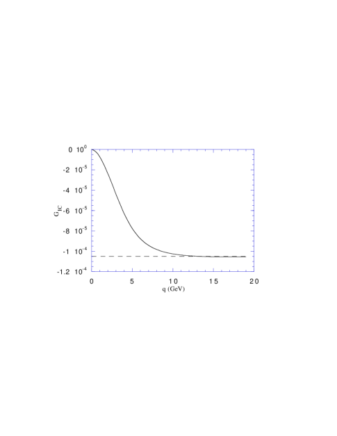
FIG. 17.: The interaction current contribution to the deuteron form factor in the case of Model 1, plotted out to very large values of $Q$. The dashed line shows the calculated value of the constant which the interaction current should approach as $Q$ becomes large.

This concludes the discussion of the specifics of the tower models.

Derivation of the interaction current

In this appendix we derive the interaction current given in Eq. (44). While the method is similar to that used in Ref. [25], there are certain differences which will be detailed here.

The interaction current will be obtained by minimal substitution, which is most easily done in coordinate space. The interaction is chosen to depend on $D$ and $p_{n}$; the coordinates conjugate to these momenta will be labeled $r$ and $r_{d}$. From

$$p\cdot r+p_{n}\cdot r_{n}=D\cdot r+p_{n}\cdot r_{d}\,,$$ (125)

it follows that $r_{d}=r_{n}-r$. Using these conjugate coordinates, the strong interaction in coordinate space can be written as (factors of $g$ are neglected for the moment)

$$\Delta = \int\frac{d^{4}p_{n}^{\prime}\,d^{4}p_{n}\,d^{4}D^{\prime}\,d^{4}D}{(2\pi)^{12}}\;e^{i(D^{\prime}\cdot r^{\prime}+p_{n}^{\prime}\cdot r_{d}^{\prime})}e^{-i(D\cdot r+p_{n}\cdot r_{d})}f(x^{\prime})f(x)\,\delta^{4}(D^{\prime}-D)$$ (126)

$$= \int\frac{d^{4}p_{n}^{\prime}\,d^{4}p_{n}\,d^{4}D}{(2\pi)^{12}}\;e^{i(D\cdot y+p_{n}^{\prime}\cdot r^{\prime}_{d}-p_{n}\cdot r_{d})}f(x^{\prime})f(x)$$ (127)

$$= \Delta(y;r_{d}^{\prime},r_{d}),$$ (128)

where $y=r^{\prime}-r$, and $x^{\prime}$ and x were defined in Eq. (8) (with $x^{\prime}$ obtained from $x$ by replacing $p_{n}$ with $p^{\prime}_{n}$). Note that in coordinate space, the strong interaction is not separable, as it is in momentum space.

Particle 2 is neutral, so dependences of the potential on $p_{n}$ and $p^{\prime}_{n}$

$$p^{\mu}_{n}=-i\frac{\partial}{\partial r_{d\;\mu}}\qquad p^{\prime\mu}_{n}=-i\frac{\partial}{\partial r^{\prime}_{d\;\mu}}$$ (129)

do not generate any current. Particle 1 is charged, and the coordinate associated with it is $y$. Therefore, from minimal substitution the dependences on $D^{\mu}$ generate

$$D^{\mu}=-i\frac{\partial}{\partial y_{\mu}}\longrightarrow-i\frac{\partial}{\partial y_{\mu}}+e\,\epsilon^{\mu}e^{iq\cdot y}.$$ (130)

Applying this to Eq. (128) generates an interaction current proportional to $\Gamma_{\mu}$

$$\Delta(y;r_{d}^{\prime},r_{d})\longrightarrow\Delta(y;r_{d}^{\prime},r_{d})+e\,\epsilon^{\mu}\,\Gamma_{\mu}(y;r_{d}^{\prime},r_{d})\,,$$ (131)

where $e\,\epsilon^{\mu}\,\Gamma_{\mu}$ is the first order (in the charge $e$) change to $\Delta$ which arises from the substitution (130). To find $\Gamma$, this change must be evaluated from

$$\delta\Delta = e\,\epsilon^{\mu}\,\Gamma_{\mu}(y;r_{d}^{\prime},r_{d})$$ (132)

$$= \int_{D}\Biggl{(}\left\{f\left[x\left(p^{\prime}_{n},-i\frac{\partial}{\partial y_{\mu}}+e\,\epsilon^{\mu}\,e^{iq\cdot y}\right)\right]f\left[x\left(p_{n},-i\frac{\partial}{\partial y_{\mu}}+e\,\epsilon^{\mu}\,e^{iq\cdot y}\right)\right]\right\}$$ (134)

$$-\left\{f\left[x\left(p^{\prime}_{n},-i\frac{\partial}{\partial y}\right)\right]f\left[x\left(p_{n},-i\frac{\partial}{\partial y}\right)\right]\right\}\Biggr{)}\;e^{i(D\cdot y+p_{n}^{\prime}\cdot r_{d}^{\prime}-p_{n}\cdot r_{d})}\,,$$

where

$$\int_{D}=\int\frac{d^{4}Dd^{4}p_{n}^{\prime}d^{4}p_{n}}{(2\pi)^{12}}\,.$$ (135)

To evaluate this, assume that $f$ can be expanded in a Taylor series

$$f(x)=\sum_{n}c_{n}\,x^{n}\,,$$ (136)

define ${\cal Z}_{\mu}$ by

$$x\left(p_{n},-i\frac{\partial}{\partial y_{\mu}}+e\epsilon^{\mu}e^{iq\cdot y}\right)=\tilde{x}=x\left(p_{n},-i\frac{\partial}{\partial y_{\mu}}\right)+e\,\epsilon^{\mu}\,{\cal Z}_{\mu}\,e^{iq\cdot y}+{\cal O}(e^{2})\,,$$ (137)

and work out the difference $\tilde{x}^{n}-x^{n}$ arising from the minimal substitution. Since $\delta\,x=\tilde{x}-x$ does not commute with $x$, this difference must first be written

$$\tilde{x}^{n}-x^{n}=\sum_{m}x^{n-1-m}\left(p_{n},-i\frac{\partial}{\partial y_{\mu}}\right)\,(\delta\,x)\,x^{m}\left(p_{n},-i\frac{\partial}{\partial y_{\mu}}\right)\,.$$ (138)

Now take into account the fact that each appearance of $\partial/\partial y$ will act on all factors of y to the right of it. This includes the factor of $\exp i(D\cdot y+p_{n}^{\prime}\cdot r_{d}-p_{n}\cdot r_{d})$ in the definition of $\delta\Delta$ where this expansion of the form factor will eventually be used. Therefore, factors of x occurring to the right of the factor $\delta\,x$ will depend on D only, while factors of x occurring to the left of the $\delta\,x$ term will depend on $D+q=D^{\prime}$ once the expansion is inserted into Eq. (134). Hence the change in $x^{n}$ under minimal substitution to first order in e is

$$\tilde{x}^{n}-x^{n}= \sum_{m}x^{n-1-m}(p_{n},D+q)\left[e\epsilon^{\mu}{\cal Z}_{\mu}e^{iq\cdot y}\right]x^{m}(p_{n},D)$$ (139)

$$= e\,\epsilon^{\mu}\,{\cal Z}_{\mu}\,e^{iq\cdot y}\;\sum_{m}x^{n-1-m}(p_{n},D+q)x^{m}(p_{n},D)\,.$$ (140)

Using the algebraic identity

$$\sum_{m=0}^{n-1}a^{n-1-m}b^{m}=\frac{a^{n}-b^{n}}{a-b},$$ (141)

Eq. (140) becomes

$$\tilde{x}^{n}-x^{n}=e\,\epsilon^{\mu}\,{\cal Z}_{\mu}\,e^{iq\cdot y}\;\frac{x^{n}(p_{n},D+q)-x^{n}(p_{n},D)}{x(p_{n},D+q)-x(p_{n},D)}\,.$$ (142)

Therefore, the change in f under minimal substitution is

$$\delta f=e\,\epsilon^{\mu}\,{\cal Z}_{\mu}\,e^{iq\cdot y}\;\frac{f\left[x(p_{n},D+q)\right]-f\left[x(p_{n},D)\right]}{x(p_{n},D+q)-x(p_{n},D,)}.$$ (143)

Note that Eq. (134) has the form $\tilde{f}^{\prime}\tilde{f}-f^{\prime}f$, where the tilde indicates the use of minimal substitution. To first order in e this can be written

$$\tilde{f}^{\prime}\tilde{f}-f^{\prime}f = \tilde{f}^{\prime}\tilde{f}-f^{\prime}\tilde{f}+f^{\prime}\tilde{f}-f^{\prime}f$$ (144)

$$= \delta f^{\prime}\tilde{f}+f^{\prime}\delta f$$ (145)

$$= \delta f^{\prime}f+f^{\prime}\delta f\,.$$ (146)

Thus, Eq. (134) becomes

$$\delta\Delta = \int_{D}e^{i\left[D^{\prime}\cdot y+p_{n}^{\prime}\cdot r_{d}^{\prime}-p_{n}\cdot r_{d}\right]}\Biggl{\{}e\,\epsilon^{\mu}\,{\cal Z}^{\prime}_{\mu}\;\frac{f\left[x(p_{n}^{\prime},D^{\prime})\right]-f\left[x(p^{\prime}_{n},D)\right]}{x(p_{n}^{\prime},D^{\prime})-x(p^{\prime}_{n},D)}f\left[x(p_{n},D)\right]$$ (148)

$$+e\,\epsilon^{\mu}\,{\cal Z}_{\mu}\;f\left[x(p_{n}^{\prime},D^{\prime})\right]\frac{f\left[x(p_{n},D^{\prime})\right]-f\left[x(p_{n},D)\right]}{x(p_{n},D^{\prime})-x(p_{n},D)}\Biggr{\}}\,.$$

Recalling that $\delta\Delta=e\,\epsilon^{\mu}\,\Gamma_{\mu}$, we can unfold the integral to give

$$j_{\mu}^{INT}=e\,g\Biggl{\{} {\cal Z}^{\prime}_{\mu}\;\frac{f\left[x(p_{n}^{\prime},D^{\prime})\right]-f\left[x(p^{\prime}_{n},D)\right]}{x(p_{n}^{\prime},D^{\prime})-x(p^{\prime}_{n},D)}f\left[x(p_{n},D)\right]$$ (150)

$$+{\cal Z}_{\mu}\,f\left[x(p_{n}^{\prime},D^{\prime})\right]\frac{f\left[x(p_{n},D^{\prime})\right]-f\left[x(p_{n},D)\right]}{x(p_{n},D^{\prime})-x(p_{n},D)}\Biggr{\}}\,,$$

which is the one-member tower version of Eq. (44).

To complete the calculation we must find ${\cal Z}^{\mu}$. We begin from its definition in Eq. (140) and construct it directly. Using the definition of $x$, Eq. (8), assuming that $\tilde{x}$ may be expanded in a power series in $e$, using the notation

$$\tilde{D}^{\mu}=-i{\partial\over\partial y_{\mu}}+e\,\epsilon^{\mu}\,e^{iq\cdot y}=-i{\partial\over\partial y_{\mu}}+e\,\delta^{\mu}\,,$$ (151)

and keeping only those terms which are first order in $e$, the change in $x$ due to minimal substitution is

$$\frac{\tilde{x}-x}{e} = -{(p_{n}\cdot\tilde{D})^{2}\over e\,\tilde{D}^{2}}+{(p_{n}\cdot{D})^{2}\over e\,{D}^{2}}$$ (152)

$$= -\left\{{1\over 2D^{2}}\;,\;\left[(p_{n}\cdot{D})\;(p_{n}\cdot\delta)+(p_{n}\cdot\delta)\;(p_{n}\cdot{D})\right]\right\}$$ (155)

$$+\left\{\lambda\;(p_{n}\cdot D)^{2}\;,\;\left[\frac{1}{4D^{4}}\left\{\delta,D\right\}+\left\{\delta,D\right\}\frac{1}{4D^{4}}\right]\right\}$$

$$+\left\{(1-\lambda)(p_{n}\cdot D)^{2}\;,\;\frac{1}{2D^{2}}\left\{\delta,D\right\}\frac{1}{D^{2}}\right\}\,,$$

where $\{A,B\}=AB+BA$, and

$$\left\{\delta,D\right\}=\left\{\epsilon\cdot D,e^{iq\cdot y}\right\}=\epsilon\cdot D\,e^{iq\cdot y}+e^{iq\cdot y}\,\epsilon\cdot D$$ (156)

is the summetrized expansion of $\tilde{D}^{2}-D^{2}$. We have expanded these functions symmetrically, using anticommutators of non-commuting operators, since every factor of $D$ contains a derivative which may not necessarily commute with all of its surrounding terms. The parameter $\lambda$ is introduced to provides a continuous choice between two different ways of symmetrizing the expansion of the $D^{-2}$ term; it is not clear a priori which of this continuous range of choices is correct. (If the operators all commuted, the result would be independent of the choice of $\lambda$.) Extracting the common factor of $\epsilon^{\mu}\,e^{iq\cdot y}$ [remembering that factors of $D$ contain derivatives which act all the way to the right when they are substituted into Eq. (134)], gives

$$\frac{\tilde{x}-x}{e} = -\epsilon^{\mu}e^{iq\cdot y}\left\{p_{n_{\mu}}\;\;\left[p_{n}\cdot(D+D^{\prime})\right]\left[\frac{1}{2D^{\prime^{2}}}+\frac{1}{2D^{2}}\right]\right\}$$ (159)

$$+\epsilon^{\mu}e^{iq\cdot y}\Biggl{\{}(D+D^{\prime})_{\mu}\left[(p_{n}\cdot D)^{2}+(p_{n}\cdot D^{\prime})^{2}\right]$$

$$\qquad\qquad\times\left[\frac{\lambda}{4}\left(\frac{1}{D^{4}}+\frac{1}{D^{\prime^{4}}}\right)+\frac{1-\lambda}{2D^{2}D^{\prime^{2}}}\right]\Biggr{\}}\,.$$

Therefore,

$${\cal Z}^{\mu} = -p_{n}^{\mu}\,\,\left[p_{n}\cdot(D+D^{\prime})\right]\left(\frac{1}{2D^{\prime^{2}}}+\frac{1}{2D^{2}}\right)$$ (161)

$$+(D+D^{\prime})^{\mu}\left[(p_{n}\cdot D)^{2}+(p_{n}\cdot D^{\prime})^{2}\right]\left[\frac{\lambda}{4}\left(\frac{1}{D^{4}}+\frac{1}{D^{\prime^{4}}}\right)+\frac{1-\lambda}{2D^{2}D^{\prime^{2}}}\right]\,.$$

All that remains is to determine $\lambda$. To do this, look at Eq. (161) in the case of elastic scattering ($D^{2}=D^{\prime^{2}}=M_{D}^{2}$). Contracting with $q$ gives

$$q_{\mu}{\cal Z}^{\mu}=-\left[(p_{n}\cdot D^{\prime})^{2}-(p_{n}\cdot D)^{2}\right]\frac{1}{M_{D}^{2}}=x(p_{n},D^{\prime})-x(p_{n},D)\,.$$ (162)

This is the result needed for the total current to be conserved [this result leads directly to Eq. (47)]. Hence, current conservation requires that this should be the result even when the scattering is not elastic. In that case,

$$q_{\mu}{\cal Z}^{\mu}= (p_{n}\cdot D^{\prime})^{2}\left[-\frac{1}{2D^{\prime^{2}}}\left(2-{3\over 2}\lambda\right)-\frac{1}{2D^{2}}\left({3\over 2}\lambda\right)+\frac{\lambda D^{\prime^{2}}}{4D^{4}}-\frac{\lambda D^{2}}{4D^{\prime^{4}}}\right]$$ (164)

$$+(p_{n}\cdot D)^{2}\left[\frac{1}{2D^{2}}\left(2-{3\over 2}\lambda\right)+\frac{1}{2D^{\prime^{2}}}\left({3\over 2}\lambda\right)+\frac{\lambda D^{\prime^{2}}}{4D^{4}}-\frac{\lambda D^{2}}{4D^{\prime^{4}}}\right]$$

Clearly the choice of $\lambda=0$ will reduce the expression to the desired form, ${\cal Z}_{\mu}$ reduces to Eq. (46), and the interaction current (150) is completely specified. The generalization of the interaction current to the case with more than one tower member is straightforward; the result is given in Eq. (44).

REFERENCES

- [1]
- [2] Based on work completed by K. Herbst in partial fulfilment of requirements for the Ph.D. degree at the College of William and Mary.
- [3] R. Reid, Ann. Phys. (N.Y.) 50, 411 (1968).
- [4] R. A. Malfliet and J. A. Tjon, Nucl. Phys. A127, 161 (1969).
- [5] L. Črepinšek, C. B. Lang, H. Oberhummer, W. Plessas, and H. F. K. Zingl, Acta Phys. Austriaca 42, 139 (1975).
- [6] R. R. Silbar and W. M. Kloet, Nucl. Phys. A338, 317 (1980).
- [7] L. Mathelitsch, W. Plessas, and W. Schweiger, Phys. Rev. C 26, 65 (1982).
- [8] K. Schwarz, J. Haidenbauer, and J. Fröhlich, Phys. Rev. C 33, 456 (1986).
- [9] W. A. Schnizer and W. Plessas, Phys. Rev. C 41, 1095 (1990).
- [10] G. Rupp and J. A. Tjon, Phys. Rev. C 45, 2133 (1992).
- [11] F. Gross, J. W. VanOrden, and K. Holinde, Phys. Rev. C 45, 2094 (1992).
- [12] J. Fleischer and J. A. Tjon, Nucl. Phys B84, 375 (1975); Phys. Rev. D 15, 2537 (1977); 21, 87 (1980).
- [13] M. J. Zuilhof and J. A. Tjon, Phys. Rev. C 22, 2369 (1980); 24, 736 (1981).
- [14] E. vanFaassen and J. A. Tjon, Phys. Rev. C 28, 2354 (1983); 30, 285 (1984).
- [15] E. vanFaassen and J. A. Tjon, Phys. Rev. C 33, 2105 (1986).
- [16] G. Rupp and J. A. Tjon, Phys. Rev. C 37, 1729 (1988).
- [17] E. E. Salpeter and H. A. Bethe, Phys. Rev. 84, 1232 (1951).
- [18] R. Blankenbecler and R. Sugar, Phys. Rev. 142, 1051 (1966).
- [19] F. Gross, Phys. Rev. 186, 1448 (1969).
- [20] F. Gross, Phys. Rev. D 10, 223 (1974).
- [21] F. Gross, Czech. J. Phys. B 39, 871 (1989).
- [22] F. Gross, Relativistic Quantum Mechanics and Field Theory (John Wiley and Sons, New York, 1993), Chap. 12.
- [23] V. G. J. Stoks, R. A. M. Klomp, M. C. M. Rentmeester, and J. J. de Swart, Phys. Rev. C 48, 792 (1993).
- [24] F. Gross and D. O. Riska, Phys. Rev. C 36, 1928 (1987).
- [25] H. Ito, W. W. Buck, and F. Gross, Phys. Rev C 43, 2483 (1991).
- [26] R. A. Arndt, L. D. Roper, R. A. Bryan, R. B. Clark, B. J. VerWest, and P. Signell, Phys. Rev. D 28, 97 (1983).
- [27] M. Garçon, et.al., Phys. Rev. C 49, 2516 (1994).
- [28] F. Gross and Y. Surya, Phys. Rev. C 47, 703 (1993). The formulation of the inelastic scattering matrix and subsequent calculations closely resemble their Appendix C.
- [29] Y. Takahashi, Nuovo Cimento 6, 2231 (1957).
- [30] J. C. Ward, Phys. Rev. 77, 293 (1950); 78, 182 (1950); Proc. Phys. Soc. 64, 54 (1951).