Electromagnetic interactions for the two-body spectator equations

Abstract

This paper presents a new non-associative algebra which is used to (i) show how the spectator (or Gross) two-body equations and electromagnetic currents can be formally derived from the Bethe-Salpeter equation and currents if both are treated to all orders, (ii) obtain explicit expressions for the Gross two-body electromagnetic currents valid to any order, and (iii) prove that the currents so derived are exactly gauge invariant when truncated consistently to any finite order. In addition to presenting these new results, this work complements and extends previous treatments based largely on the analysis of sums of Feynman diagrams.

I Introduction

The two-body spectator (or Gross) equations were first introduced in 1969 and have been developed in a number of subsequent papers [1]. The treatment of electromagnetic interactions in this context has also been studied [2]–[5]. However, all of these previous treatments have been largely based on the analysis of Feynman diagrams, and the equations have been largely derived from this diagrammatic analysis. In this paper we present an algebraic derivation of the equations which is complementary to previous diagrammatic derivations. More specifically, we develop a new operator algebra which involves some non-associative rules for the treatment of products of singular operators. Once this operator algebra has been carefully defined and developed, it provides a powerful tool for the formal manipulation of the equations and permits a careful and detailed comparison with the Bethe-Salpeter equations. It also alows us to derive several new results which would be difficult to derive using a purely diagrammatic approach. In applications the relativistic kernel for either the Bethe-Salpeter equation or the Gross equation is usually expanded in a perturbation series, and in this paper we obtain, for the first time, the form of the electromagnetic current operator for the Gross equation which is valid to all orders in this expansion. We also show explicitly that the theory conserves the charge of a bound state, and that gauge invariance is exactly preserved when the theory is truncated to any finite order, provided only that the strong kernel and the electromagnetic current operator are both truncated to the same finite order.

This work is a continuation of recent work [6] in which the normalization condition for the three-body vertex function was derived, and also lays the foundation for extension of recent developments of the three-body Gross equations by Stadler and Gross [7]. The new algebra developed in this paper will be used to derive, in this forthcoming paper, the electromagnetic current operator for the three-body Gross equations [8], and we have developed the formalism here with an eye to this extension. Spectator currents have also been independently discussed by Kvinikhidze and Blankleider [9]. Their discussion is more limited in scope than ours (here we develop an operator algebra, discuss the connection with the Bethe-Salpeter equation, and obtain results to all orders), but the results they do obtain agree with us (see the discussion in Sec. III below).

A number of other works deriving the electromagnetic current for various relativistic equations have appeared recently. Coester and Riska have derived the current operator for the Blankenbecler-Sugar equation [10] and Devine and Wallace [11] and Phillips and Wallace [12] have discussed the construction of a current operator for use with a relativistic version of the equal time equation. Extension of the new operator formalism presented here to these other equations is being studied. This effort may clarify a number of issues still unresolved in these treatments.

This paper begins with a brief review of the Bethe-Salpeter equation and the corresponding current operator. In Sec. III we extend this discussion to the Gross equation, in both the unsymmetrized form for nonidentical particles and the symmetrized form appropriate for the description of identical particles. In Sec. IV we present the final form for the currents and show that the currents appropriate for identical and nonidentical particles are equivalent. We also show that the exact results in the two formalisms (BS and spectator) are identical if both are calculated to all orders. Then, in Sec. V we use the normalization conditions proved in a previous paper [6] to show that the charge of the bound state is conserved by both theories. In Sec. VI we discuss the results when the perturbation expansions for the kernel and the current operator are truncated to a finite order, and show that gauge invariance is still satisfied. Finally, conclusions are presented in Sec. VII.

II Two-body Bethe-Salpeter Equation

In this section we review the Bethe-Salpeter formalism. Our results are not new, but the brief systematic development given here is needed both as an introduction to what will follow, and as a description of the formalism to which the spectator results will be compared. To prepare the way, we develop the subject using a conventional operator formalism. The need for non-associative operators will not appear until the next section.

The operator form of the equation for the four-point propagator as represented in Fig. 1 is

$${\cal G}= G_{\rm BS}-G_{\rm BS}V{\cal G}$$ (1)

$$= G_{\rm BS}-{\cal G}VG_{\rm BS}\,,$$ (2)

where the free two-body propagator $G_{\rm BS}=-iG_{1}G_{2}$ is defined in terms of the single-particle propagators $G_{i}$ and $V$ is the two-body Bethe-Salpeter kernel.

The usual momentum-space forms of these expressions can be obtained by introducing the virtual momentum space states defined such that

$$\left<x\right|\left.p\right> = e^{i\mathchoice{{\hbox{\boldmath$\displaystyle p$}}}{{\hbox{\boldmath$\textstyle p$}}}{{\hbox{\boldmath$\scriptstyle p$}}}{{\hbox{\boldmath$\scriptscriptstyle p$}}}\cdot\mathchoice{{\hbox{\boldmath$\displaystyle x$}}}{{\hbox{\boldmath$\textstyle x$}}}{{\hbox{\boldmath$\scriptstyle x$}}}{{\hbox{\boldmath$\scriptscriptstyle x$}}}-ip^{0}t}\,,$$ (3)

$$\left<p^{\prime}\right|\left.p\right> = (2\pi)^{4}\delta^{4}(p^{\prime}-p)$$ (4)

and

FIG. 1.: Diagrammatic representation of the integral equation for the four-point propagator.

$$\int\frac{d^{4}p}{(2\pi)^{4}}\left|p\right>\left<p\right|=1\,.$$ (5)

The operators are defined such that the momentum matrix elements for the one-body propagators are

$$\left<p^{\prime}_{i}|G_{i}|p_{i}\right>=G_{i}(p_{i})(2\pi)^{4}\delta^{4}(p^{\prime}_{i}-p_{i})\,,$$ (6)

the interaction kernel is

$$\left<p^{\prime}_{1}p^{\prime}_{2}|V|p_{1}p_{2}\right>=V(p^{\prime},p;P)(2\pi)^{4}\delta^{4}(P^{\prime}-P)\,,$$ (7)

and the interacting two-body propagator is

$$\left<p^{\prime}_{1}p^{\prime}_{2}|{\cal G}|p_{1}p_{2}\right>={\cal G}(p^{\prime},p;P)(2\pi)^{4}\delta^{4}(P^{\prime}-P)\,,$$ (8)

where $P=p_{1}+p_{2}$ and $P^{\prime}=p^{\prime}_{1}+p^{\prime}_{2}$ are the total momenta in the initial and final states, and $p=\frac{1}{2}(p_{1}-p_{2})$ and $p^{\prime}=\frac{1}{2}(p^{\prime}_{1}-p^{\prime}_{2})$ are the corresponding relative momenta.

The two-body propagator can also be written

$${\cal G}=G_{\rm BS}-G_{\rm BS}{\cal M}G_{\rm BS}$$ (9)

where

$${\cal M}=V-VG_{\rm BS}{\cal M}=V-{\cal M}G_{\rm BS}V$$ (10)

is the two-body scattering matrix. The Bethe-Salpeter equation for the scattering matrix (10) is represented by the Feynman diagrams of Fig. 2.

FIG. 2.: Diagrammatic representation the Bethe-Salpeter equation for the two-body scattering matrix.

Equation (1) can be written as

$$\left(G^{-1}_{\rm BS}+V\right){\cal G}=1$$ (11)

which implies that the solution for the inverse propagator is

$${\cal G}^{-1}=G^{-1}_{\rm BS}+V\,.$$ (12)

The equation for the Bethe-Salpeter bound-state vertex function is

$$\left|\Gamma\right>=-VG_{\rm BS}\left|\Gamma\right>\,,$$ (13)

which can be written

$$0=\left(1+VG_{\rm BS}\right)\left|\Gamma\right>=\left(G_{\rm BS}^{-1}+V\right)G_{\rm BS}\left|\Gamma\right>\,.$$ (14)

Using (12) this can be written

$${\cal G}^{-1}\left|\psi\right>=0\,,$$ (15)

where the Bethe-Salpeter bound-state wave function is defined as

$$\left|\psi\right>=G_{\rm BS}\left|\Gamma\right>\,.$$ (16)

The scattering states are defined in terms of physical, on-shell states with the normalization

$$\left<x\right|\left.\mathchoice{{\hbox{\boldmath$\displaystyle p$}}}{{\hbox{\boldmath$\textstyle p$}}}{{\hbox{\boldmath$\scriptstyle p$}}}{{\hbox{\boldmath$\scriptscriptstyle p$}}}\right>=e^{i\mathchoice{{\hbox{\boldmath$\displaystyle p$}}}{{\hbox{\boldmath$\textstyle p$}}}{{\hbox{\boldmath$\scriptstyle p$}}}{{\hbox{\boldmath$\scriptscriptstyle p$}}}\cdot\mathchoice{{\hbox{\boldmath$\displaystyle x$}}}{{\hbox{\boldmath$\textstyle x$}}}{{\hbox{\boldmath$\scriptstyle x$}}}{{\hbox{\boldmath$\scriptscriptstyle x$}}}-iE_{p}t}$$ (17)

where $E_{p}=\sqrt{\mathchoice{{\hbox{\boldmath$\displaystyle p$}}}{{\hbox{\boldmath$\textstyle p$}}}{{\hbox{\boldmath$\scriptstyle p$}}}{{\hbox{\boldmath$\scriptscriptstyle p$}}}^{2}+m^{2}}$. To include spin, we define the asymptotic single-particle plane wave momentum state as

$$\left|\mathchoice{{\hbox{\boldmath$\displaystyle p$}}}{{\hbox{\boldmath$\textstyle p$}}}{{\hbox{\boldmath$\scriptstyle p$}}}{{\hbox{\boldmath$\scriptscriptstyle p$}}},s\right>=\left\{\begin{array}[]{ll}u(\mathchoice{{\hbox{\boldmath$\displaystyle p$}}}{{\hbox{\boldmath$\textstyle p$}}}{{\hbox{\boldmath$\scriptstyle p$}}}{{\hbox{\boldmath$\scriptscriptstyle p$}}},s)\left|\mathchoice{{\hbox{\boldmath$\displaystyle p$}}}{{\hbox{\boldmath$\textstyle p$}}}{{\hbox{\boldmath$\scriptstyle p$}}}{{\hbox{\boldmath$\scriptscriptstyle p$}}}\right>&\quad{\rm for\ spin}=\frac{1}{2}\\ \left|\mathchoice{{\hbox{\boldmath$\displaystyle p$}}}{{\hbox{\boldmath$\textstyle p$}}}{{\hbox{\boldmath$\scriptstyle p$}}}{{\hbox{\boldmath$\scriptscriptstyle p$}}}\right>&\quad{\rm for\ spin}=0\end{array}\right.$$ (18)

The final state Bethe-Salpeter scattering wave function with incoming spherical wave boundary conditions is then

$$\left<\psi^{(-)}\right|=\left<\mathchoice{{\hbox{\boldmath$\displaystyle p$}}}{{\hbox{\boldmath$\textstyle p$}}}{{\hbox{\boldmath$\scriptstyle p$}}}{{\hbox{\boldmath$\scriptscriptstyle p$}}}_{1},s_{1};\mathchoice{{\hbox{\boldmath$\displaystyle p$}}}{{\hbox{\boldmath$\textstyle p$}}}{{\hbox{\boldmath$\scriptstyle p$}}}{{\hbox{\boldmath$\scriptscriptstyle p$}}}_{2},s_{2}\right|\left(1-{\cal M}G_{\rm BS}\right)\,.$$ (19)

Using this

$$\left<\psi^{(-)}\right|{\cal G}^{-1} = \left<\mathchoice{{\hbox{\boldmath$\displaystyle p$}}}{{\hbox{\boldmath$\textstyle p$}}}{{\hbox{\boldmath$\scriptstyle p$}}}{{\hbox{\boldmath$\scriptscriptstyle p$}}}_{1},s_{1};\mathchoice{{\hbox{\boldmath$\displaystyle p$}}}{{\hbox{\boldmath$\textstyle p$}}}{{\hbox{\boldmath$\scriptstyle p$}}}{{\hbox{\boldmath$\scriptscriptstyle p$}}}_{2},s_{2}\right|\left(1-{\cal M}G_{\rm BS}\right)\left(G^{-1}_{\rm BS}+V\right)$$ (20)

$$= \left<\mathchoice{{\hbox{\boldmath$\displaystyle p$}}}{{\hbox{\boldmath$\textstyle p$}}}{{\hbox{\boldmath$\scriptstyle p$}}}{{\hbox{\boldmath$\scriptscriptstyle p$}}}_{1},s_{1};\mathchoice{{\hbox{\boldmath$\displaystyle p$}}}{{\hbox{\boldmath$\textstyle p$}}}{{\hbox{\boldmath$\scriptstyle p$}}}{{\hbox{\boldmath$\scriptscriptstyle p$}}}_{2},s_{2}\right|\left(G^{-1}_{\rm BS}-{\cal M}+V-{\cal M}G_{\rm BS}V\right)=0\,,$$ (21)

where (10) and $\left<\mathchoice{{\hbox{\boldmath$\displaystyle p$}}}{{\hbox{\boldmath$\textstyle p$}}}{{\hbox{\boldmath$\scriptstyle p$}}}{{\hbox{\boldmath$\scriptscriptstyle p$}}}_{1},s_{1};\mathchoice{{\hbox{\boldmath$\displaystyle p$}}}{{\hbox{\boldmath$\textstyle p$}}}{{\hbox{\boldmath$\scriptstyle p$}}}{{\hbox{\boldmath$\scriptscriptstyle p$}}}_{2},s_{2}\right|G^{-1}_{\rm BS}=0$ have been used in the last step. Similarly, the initial state scattering wave function with outgoing spherical wave boundary conditions

$$\left|\psi^{(+)}\right>=\left(1-G_{\rm BS}{\cal M}\right)\left|\mathchoice{{\hbox{\boldmath$\displaystyle p$}}}{{\hbox{\boldmath$\textstyle p$}}}{{\hbox{\boldmath$\scriptstyle p$}}}{{\hbox{\boldmath$\scriptscriptstyle p$}}}_{1},s_{1};\mathchoice{{\hbox{\boldmath$\displaystyle p$}}}{{\hbox{\boldmath$\textstyle p$}}}{{\hbox{\boldmath$\scriptstyle p$}}}{{\hbox{\boldmath$\scriptscriptstyle p$}}}_{2},s_{2}\right>$$ (22)

satisfies the wave equation

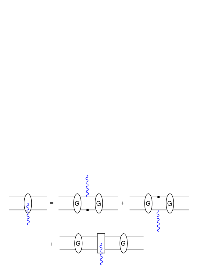
FIG. 3.: Feynman diagrams representing the five-point propagator. Inverse one-body propagators are represented by the small, solid, square boxes inserted on the propagator lines.

$${\cal G}^{-1}\left|\psi^{(+)}\right>=0\,.$$ (23)

So the two-body Bethe-Salpeter wave functions for both bound and scattering states satisfy the equation

$${\cal G}^{-1}\left|\psi\right>=\left<\psi\right|{\cal G}^{-1}=0\,.$$ (24)

The two body current can be obtained from the five-point function describing the interaction of a photon (with the photon leg amputated) with the interacting two-body system. This is represented by the diagrams of Fig. 3, and corresponds to the operator equation

$${\cal G}^{\mu}=-{\cal G}\left(iJ^{\mu}_{1}G^{-1}_{2}+iJ^{\mu}_{2}G^{-1}_{1}+J^{\mu}_{\rm ex}\right){\cal G}$$ (25)

where the inverse one-body propagators are introduced to allow for the factorization in terms of interacting four-point propagators. The inverse one-body propagators are represented by the square boxes inserted on the propagator lines in Fig. 3.

In order to demonstrate that the current

$$J^{\mu}=iJ^{\mu}_{1}G^{-1}_{2}+iJ^{\mu}_{2}G^{-1}_{1}+J^{\mu}_{\rm ex}=J^{\mu}_{\rm IA}+J^{\mu}_{\rm ex}$$ (26)

is conserved, we must introduce the one- and two-body Ward-Takahashi identities in operator form

$$q_{\mu}J^{\mu}_{i}=\left[e_{i}(q),G^{-1}_{i}\right]$$ (27)

and

$$q_{\mu}J^{\mu}_{\rm ex}=[e_{1}(q)+e_{2}(q),V]$$ (28)

where $e_{i}(q)$ is the product of the charge $e_{i}$ (which might be an operator in isospin space) and a four-momentum shift operator defined such that

$$\left<p^{\prime}_{i}|e_{i}(q)|p_{i}\right>=e_{i}(2\pi)^{4}\delta^{4}(p^{\prime}_{i}-p_{i}-q)\,.$$ (29)

Using the one- and two-body Ward-Takahashi identities give the following relation

$$q_{\mu}J^{\mu} = i\left[e_{1}(q),G^{-1}_{1}\right]G^{-1}_{2}+i\left[e_{2}(q),G^{-1}_{2}\right]G^{-1}_{1}+\left[e_{1}(q)+e_{2}(q),V\right]$$ (30)

$$= \left[e_{1}(q)+e_{2}(q),G^{-1}_{\rm BS}+V\right]=\left[e_{1}(q)+e_{2}(q),{\cal G}^{-1}\right]\,.$$ (31)

This along with (24) implies that the two-body current is conserved

$$q_{\mu}\left<\psi|J^{\mu}|\psi\right>=0\,.$$ (32)

For identical particles, the Bethe-Salpeter equation can be rewritten in an explicitly symmetrized form

$$M=\overline{V}-\overline{V}G_{\rm BS}M=\overline{V}-MG_{\rm BS}\overline{V}$$ (33)

where $\overline{V}={\cal A}_{2}V$, $M={\cal A}_{2}{\cal M}$ and ${\cal A}_{2}=\frac{1}{2}\left(1+\zeta{\cal P}_{12}\right)$ is the two-body symmetrization operator. (Note that Roman letters (e.g. $M$) are used for symmetrized quantities and script letters (e.g. ${\cal M}$) for unsymmetrized quantities, as in Ref. [6]). The corresponding four-point propagator is

$$G={\cal A}_{2}G_{\rm BS}-G_{\rm BS}\overline{V}G={\cal A}_{2}G_{\rm BS}-G_{\rm BS}MG_{\rm BS}$$ (34)

where $G={\cal A}_{2}{\cal G}$. The five-point function is also symmetrized in a similar fashion

$$G^{\mu} = -G\left(iJ^{\mu}_{1}G^{-1}_{2}+iJ^{\mu}_{2}G^{-1}_{1}+\overline{J}^{\mu}_{\rm ex}\right)G$$ (35)

$$= -{\cal A}_{2}\left(G_{\rm BS}-G_{\rm BS}MG_{\rm BS}\right)\left(iJ^{\mu}_{1}G^{-1}_{2}+iJ^{\mu}_{2}G^{-1}_{1}+\overline{J}^{\mu}_{\rm ex}\right)\left(G_{\rm BS}-G_{\rm BS}MG_{\rm BS}\right)$$ (36)

where $\overline{J}^{\mu}_{\rm ex}={\cal A}_{2}J^{\mu}_{\rm ex}$ and satisfies the Ward-Takahashi identity

$$q_{\mu}\overline{J}^{\mu}_{\rm ex}=[e_{1}(q)+e_{2}(q),\overline{V}].$$ (37)

The proof of current conservation follows in exactly the same way as for the unsymmetrized case.

III The Two-Body Gross Equation

In order to extend this discussion to the spectator or Gross equation, it is useful to examine the connection of the Gross equation to the Bethe-Salpeter equation. This is done most easily for the case of nonidentical particles. Identical particles will be discussed later.

A Two-Body Equations for Distinguishable Particles

In order to introduce the singular operators needed for our discussion and to derive their non-associative operator algebra, we first review the procedure used to motivate the rearrangement of the multiple scattering series which leads to the Gross equation. This is illustrated by considering the second-order box diagram of Fig. 4 which represents the interaction of two particles through the exchange of two light bosons. We assume the two particles to be of different masses, with the heavier mass associated with particle 1. The location of the 8 poles in the energy loop integration is shown in Fig. 5. Here the positive and negative energy poles of interacting particles 1 and 2 are labeled $1^{\pm}$ and $2^{\pm}$ and the poles in the propagators of the exchanged bosons are unlabeled. For low energies the loop integral will be dominated by the the two poles $1^{+}$ and $2^{+}$, which lie close to each other (and pinch above the scattering threshold). If the contour of integration is closed in the lower half-plane the result is dominated by the contribution from $1^{+}$, the positive energy pole for particle 1.

FIG. 4.: The box diagram.

This suggests that it may be reasonable to separate the contour integration into two contributions, one containing only the contribution from the positive energy pole for particle 1 and one containing contributions from all of the remaining poles within the contour.

This separation into two terms is best illustrated by considering the Dirac propagator for a single particle

$$G = \int\frac{d^{4}p}{(2\pi)^{4}}\left|p\right>\frac{1}{m-\not\!p-i\epsilon}\left<p\right|$$ (38)

$$= \int\frac{d^{4}p}{(2\pi)^{4}}\left|p\right>\frac{m}{E_{p}}\left[\frac{\Lambda^{+}(\mathchoice{{\hbox{\boldmath$\displaystyle p$}}}{{\hbox{\boldmath$\textstyle p$}}}{{\hbox{\boldmath$\scriptstyle p$}}}{{\hbox{\boldmath$\scriptscriptstyle p$}}})}{E_{p}-p^{0}-i\epsilon}+\frac{\Lambda^{-}(-\mathchoice{{\hbox{\boldmath$\displaystyle p$}}}{{\hbox{\boldmath$\textstyle p$}}}{{\hbox{\boldmath$\scriptstyle p$}}}{{\hbox{\boldmath$\scriptscriptstyle p$}}})}{E_{p}+p^{0}-i\epsilon}\right]\left<p\right|\,,$$ (39)

where

$$\Lambda^{\pm}(\mathchoice{{\hbox{\boldmath$\displaystyle p$}}}{{\hbox{\boldmath$\textstyle p$}}}{{\hbox{\boldmath$\scriptstyle p$}}}{{\hbox{\boldmath$\scriptscriptstyle p$}}})={m\pm(E_{p}\gamma^{0}-\mathchoice{{\hbox{\boldmath$\displaystyle p$}}}{{\hbox{\boldmath$\textstyle p$}}}{{\hbox{\boldmath$\scriptstyle p$}}}{{\hbox{\boldmath$\scriptscriptstyle p$}}}^{i}\gamma^{i})\over 2m}$$ (40)

are the positive and negative energy projection operators. If we subtract the the Dirac conjugate

$${\Lambda^{+}(\mathchoice{{\hbox{\boldmath$\displaystyle p$}}}{{\hbox{\boldmath$\textstyle p$}}}{{\hbox{\boldmath$\scriptstyle p$}}}{{\hbox{\boldmath$\scriptscriptstyle p$}}})\over E_{p}-p^{0}+i\epsilon}$$ (41)

from the first term on the right hand side of (39) and add it to the second term we obtain

$$G = \int\frac{d^{4}p}{(2\pi)^{4}}\left|p\right>\left[\frac{m}{E_{p}}\frac{2i\epsilon\Lambda^{+}(\mathchoice{{\hbox{\boldmath$\displaystyle p$}}}{{\hbox{\boldmath$\textstyle p$}}}{{\hbox{\boldmath$\scriptstyle p$}}}{{\hbox{\boldmath$\scriptscriptstyle p$}}})}{\left(E_{p}-p^{0}\right)^{2}+\epsilon^{2}}+\frac{\not\!p+m}{\left(E_{p}-p^{0}+i\epsilon\right)\left(E_{p}+p^{0}-i\epsilon\right)}\right]\left<p\right|\,.$$ (42)

The first and second terms on the right hand side of this equation are represented by the left and right hand diagrams in Fig. 6, respectively. The first term contains a new pole which is the conjugate to $1^{+}$, lies just above the real axis, and pinches the pole at $1^{+}$ when the limit $\epsilon\to 0$ is taken. As we will see below, this automatically selects the positive energy pole for particle 1. The second term is a difference propagator corresponding to the second diagram in Fig. 6. It is the same as the original propagator but with pole $1^{+}$ moved above the real axis. If we now define

FIG. 5.: Location of the 8 propagator poles in the integrand of the box diagram in the complex $p_{0}$ plane (where $p_{0}$ is the relative energy of the two internal particles).

FIG. 6.: The singularities of the two contributions to the box diagram resulting from the decomposition of $G_{1}$ into ${\cal Q}_{1}$ (left panel) and $\Delta G_{1}$ (right panel). The role of the additional singularity $1^{+}$ in the upper half plane in the left panel is to pinch the contour. Mathematically this puts particle 1 on-shell.

$${\cal Q}=\int\frac{d^{4}p}{(2\pi)^{4}}\left|p\right>\frac{N}{2E_{p}}\frac{2\epsilon Q(\mathchoice{{\hbox{\boldmath$\displaystyle p$}}}{{\hbox{\boldmath$\textstyle p$}}}{{\hbox{\boldmath$\scriptstyle p$}}}{{\hbox{\boldmath$\scriptscriptstyle p$}}})}{\left(E_{p}-p^{0}\right)^{2}+\epsilon^{2}}\left<p\right|$$ (43)

and

$$\Delta G=\int\frac{d^{4}p}{(2\pi)^{4}}\left|p\right>\frac{L(p)}{\left(E_{p}-p^{0}+i\epsilon\right)\left(E_{p}+p^{0}-i\epsilon\right)}\left<p\right|\,,$$ (44)

where

$$N=\left\{\begin{array}[]{ll}2m&{\rm for\ spin}=\frac{1}{2}\\ 1&{\rm for\ spin}=0\,,\end{array}\right.$$ (45)

$$Q(\mathchoice{{\hbox{\boldmath$\displaystyle p$}}}{{\hbox{\boldmath$\textstyle p$}}}{{\hbox{\boldmath$\scriptstyle p$}}}{{\hbox{\boldmath$\scriptscriptstyle p$}}})=\left\{\begin{array}[]{ll}\Lambda^{+}(\mathchoice{{\hbox{\boldmath$\displaystyle p$}}}{{\hbox{\boldmath$\textstyle p$}}}{{\hbox{\boldmath$\scriptstyle p$}}}{{\hbox{\boldmath$\scriptscriptstyle p$}}})&{\rm for\ spin}=\frac{1}{2}\\ 1&{\rm for\ spin}=0\,,\end{array}\right.$$ (46)

and

$$L(p)=\left\{\begin{array}[]{ll}\not\!p+m&{\rm for\ spin}=\frac{1}{2}\\ 1&{\rm for\ spin}=0\,,\end{array}\right.$$ (47)

we see that the propagator for particle $i$ has been separated into two pieces

$$G_{i}=i{\cal Q}_{i}+\Delta G_{i}\,.$$ (48)

Furthermore, using contour integration it is easy to show that

$$\lim_{\epsilon\rightarrow 0}{\cal Q}= \lim_{\epsilon\rightarrow 0}\int^{\infty}_{-\infty}\frac{dp^{0}}{2\pi}\int\frac{d^{3}p}{(2\pi)^{3}}\left|p\right>\frac{N}{2E_{p}}\frac{2\epsilon Q(\mathchoice{{\hbox{\boldmath$\displaystyle p$}}}{{\hbox{\boldmath$\textstyle p$}}}{{\hbox{\boldmath$\scriptstyle p$}}}{{\hbox{\boldmath$\scriptscriptstyle p$}}})}{\left(E_{p}-p^{0}\right)^{2}+\epsilon^{2}}\left<p\right|$$ (49)

$$= \int\frac{d^{3}p}{(2\pi)^{3}}\frac{N}{2E_{p}}\left|\mathchoice{{\hbox{\boldmath$\displaystyle p$}}}{{\hbox{\boldmath$\textstyle p$}}}{{\hbox{\boldmath$\scriptstyle p$}}}{{\hbox{\boldmath$\scriptscriptstyle p$}}}\right>Q(\mathchoice{{\hbox{\boldmath$\displaystyle p$}}}{{\hbox{\boldmath$\textstyle p$}}}{{\hbox{\boldmath$\scriptstyle p$}}}{{\hbox{\boldmath$\scriptscriptstyle p$}}})\left<\mathchoice{{\hbox{\boldmath$\displaystyle p$}}}{{\hbox{\boldmath$\textstyle p$}}}{{\hbox{\boldmath$\scriptstyle p$}}}{{\hbox{\boldmath$\scriptscriptstyle p$}}}\right|=\sum_{s}\int\frac{d^{3}p}{(2\pi)^{3}}\frac{N}{2E_{p}}\left|\mathchoice{{\hbox{\boldmath$\displaystyle p$}}}{{\hbox{\boldmath$\textstyle p$}}}{{\hbox{\boldmath$\scriptstyle p$}}}{{\hbox{\boldmath$\scriptscriptstyle p$}}},s\right>\left<\mathchoice{{\hbox{\boldmath$\displaystyle p$}}}{{\hbox{\boldmath$\textstyle p$}}}{{\hbox{\boldmath$\scriptstyle p$}}}{{\hbox{\boldmath$\scriptscriptstyle p$}}},s\right|\,.$$ (50)

This shows that ${\cal Q}$ acts to place the propagating particle on mass shell and contains the projection operator $Q=Q^{2}$ on to positive energy spinor states, where appropriate. Be warned that Refs. [6] and [7] did not make the distinction between ${\cal Q}$ and $Q$ being made in this paper and that their ${\cal Q}$ is the same as our $Q$. However, because of the conventions (61) to be introduced below (which were implicit in Refs. [6] and [7]), this difference does not affect the conclusions previously reached in these papers and our results are consistent with these earlier references.

While the introduction of the operator ${\cal Q}$ may seem straightforward, it is a singular operator and great care must be taken when using it. In particular, like the familiar delta function, its square is not defined. Later, we will be faced with the problem of how to treat quantities which naively appear to be products of singular operators, or a vanishing operator times a singular operator, and we will introduce a non-associative algebra for treating these products. Until then, the analysis is straightforward.

Using (48), the Bethe-Salpeter equation (10) for the t-matrix can now be formally separated into a pair of coupled equations. The first of these is

$${\cal M}=U-U{\cal Q}_{1}G_{2}{\cal M}=U-U{\cal Q}_{1}g_{1}{\cal M}\,,$$ (51)

or alternately

$${\cal M}=U-{\cal M}{\cal Q}_{1}g_{1}U\,,$$ (52)

where $U$ is called the quasipotential. The second equation relates the quasipotential to the BS kernel $V$. This equation is derived by requiring that the scattering matrix ${\cal M}$ as given by (51) be identical to that of (10). The resulting equation for the quasipotential is then

$$U=V-V(-i\Delta G_{1}G_{2})U=V-V\Delta g_{1}U=V-U\Delta g_{1}V\,.$$ (53)

Note that we use the notation

$$g_{1}= G_{2}$$ (54)

$$\Delta g_{1}= -i\Delta G_{1}G_{2}\,,$$ (55)

where the propagator with particle 1 on shell is $g_{1}=G_{2}$. [We find it convenient to label the two-body propagator by the on-shell particle and to distribute the singular factor of ${\cal Q}_{1}$ which accompanies it to other parts of the equation (as discussed below). We have therefore introduced the lower case notation (i.e. $g_{1}$) to distinguish the off-shell part of the two-body propagator from the one body propagator $G_{2}$.]

The pair of equations (51) and (53), as represented in Figs. 7 and Fig. 8, constitute a resummation of the multiple scattering series represented by (10) and are exactly equivalent to it by construction. The constrained propagator ${\cal Q}_{1}g_{1}$ in (51) limits the phase space available to particle 1 to the positive energy mass shell. Contributions from the remainder of phase space for particle 1 are included in the quasipotential (53) through the difference propagator $\Delta g_{1}$.

FIG. 7.: Feynman diagrams representing the Gross equation for the two-body scattering matrix. The cross on a propagator line designates that that propagator has been placed on its positive energy mass shell.

FIG. 8.: Feynman diagrams representing the quasipotential equation. The open circle on a propagator line represents the difference propagator.

Using (50) in (51) gives

$${\cal M} = U-U\int\frac{d^{3}p_{1}}{(2\pi)^{3}}\frac{N}{2E_{p_{1}}}\left|\mathchoice{{\hbox{\boldmath$\displaystyle p$}}}{{\hbox{\boldmath$\textstyle p$}}}{{\hbox{\boldmath$\scriptstyle p$}}}{{\hbox{\boldmath$\scriptscriptstyle p$}}}_{1}\right>Q_{1}(\mathchoice{{\hbox{\boldmath$\displaystyle p$}}}{{\hbox{\boldmath$\textstyle p$}}}{{\hbox{\boldmath$\scriptstyle p$}}}{{\hbox{\boldmath$\scriptscriptstyle p$}}}_{1})\left<\mathchoice{{\hbox{\boldmath$\displaystyle p$}}}{{\hbox{\boldmath$\textstyle p$}}}{{\hbox{\boldmath$\scriptstyle p$}}}{{\hbox{\boldmath$\scriptscriptstyle p$}}}_{1}\right|g_{1}{\cal M}$$ (56)

$$= U-U\sum_{s_{1}}\int\frac{d^{3}p_{1}}{(2\pi)^{3}}\frac{N}{2E_{p_{1}}}\left|\mathchoice{{\hbox{\boldmath$\displaystyle p$}}}{{\hbox{\boldmath$\textstyle p$}}}{{\hbox{\boldmath$\scriptstyle p$}}}{{\hbox{\boldmath$\scriptscriptstyle p$}}}_{1},s_{1}\right>\left<\mathchoice{{\hbox{\boldmath$\displaystyle p$}}}{{\hbox{\boldmath$\textstyle p$}}}{{\hbox{\boldmath$\scriptstyle p$}}}{{\hbox{\boldmath$\scriptscriptstyle p$}}}_{1},s_{1}\right|g_{1}{\cal M}\,.$$ (57)

Note that the projector ${\cal Q}_{1}$ has introduced a sum over all on-shell intermediate states for particle 1. In order to avoid the necessity of repeatedly writing the on-shell states and the associated sum, we will now introduce a notational convention. We will use the operator $Q_{1}$ to denote the presence of on-shell states acting on adjacent operators. If $Q_{1}$ appears between two other operators and therefore acts to both the left and right, on-shell states acting to both the left and right are assumed to be present. In addition the phase-space integral

$$\sum_{s_{1}}\int\frac{d^{3}p_{1}}{(2\pi)^{3}}\frac{N}{2E_{p_{1}}}$$ (58)

is also assumed to be present. If $Q_{1}$ appears as the first or last in a string of operators and therefore acts to the right or left respectively, then only the corresponding on-shell states acting to the right or left are assumed. In this case no phase-space integral is assumed. That is,

$${\cal O}^{\prime}Q_{1}{\cal O} \Rightarrow {\cal O}^{\prime}\sum_{s_{1}}\int\frac{d^{3}p_{1}}{(2\pi)^{3}}\frac{N}{2E_{p_{1}}}\left|\mathchoice{{\hbox{\boldmath$\displaystyle p$}}}{{\hbox{\boldmath$\textstyle p$}}}{{\hbox{\boldmath$\scriptstyle p$}}}{{\hbox{\boldmath$\scriptscriptstyle p$}}}_{1},s_{1}\right>\left<\mathchoice{{\hbox{\boldmath$\displaystyle p$}}}{{\hbox{\boldmath$\textstyle p$}}}{{\hbox{\boldmath$\scriptstyle p$}}}{{\hbox{\boldmath$\scriptscriptstyle p$}}}_{1},s_{1}\right|{\cal O}={\cal O}^{\prime}{\cal Q}_{1}\,{\cal O}$$ (59)

$${\cal O}Q_{1} \Rightarrow {\cal O}\left|\mathchoice{{\hbox{\boldmath$\displaystyle p$}}}{{\hbox{\boldmath$\textstyle p$}}}{{\hbox{\boldmath$\scriptstyle p$}}}{{\hbox{\boldmath$\scriptscriptstyle p$}}}_{1},s_{1}\right>$$ (60)

$$Q_{1}{\cal O} \Rightarrow \left<\mathchoice{{\hbox{\boldmath$\displaystyle p$}}}{{\hbox{\boldmath$\textstyle p$}}}{{\hbox{\boldmath$\scriptstyle p$}}}{{\hbox{\boldmath$\scriptscriptstyle p$}}}_{1},s_{1}\right|{\cal O}$$ (61)

where ${\cal O}^{\prime}$ and ${\cal O}$ represent any nonsingular operators or string of operators. One consequence of this convention is the relation

$${\cal O}^{\prime}\,Q_{1}\,{\cal Q}_{1}\,{\cal O}={\cal O}^{\prime}\,{\cal Q}_{1}\,Q_{1}\,{\cal O}={\cal O}^{\prime}\,{\cal Q}_{1}{\cal O}\,,$$ (62)

which follows from the observation that $Q_{1}\left|\mathchoice{{\hbox{\boldmath$\displaystyle p$}}}{{\hbox{\boldmath$\textstyle p$}}}{{\hbox{\boldmath$\scriptstyle p$}}}{{\hbox{\boldmath$\scriptscriptstyle p$}}}_{1},s_{1}\right>=\left|\mathchoice{{\hbox{\boldmath$\displaystyle p$}}}{{\hbox{\boldmath$\textstyle p$}}}{{\hbox{\boldmath$\scriptstyle p$}}}{{\hbox{\boldmath$\scriptscriptstyle p$}}}_{1},s_{1}\right>$. Using the convention (61), we can rewrite (57) as

$${\cal M}= U-UQ_{1}g_{1}{\cal M}$$ (63)

$$= U-{\cal M}Q_{1}g_{1}U\,.$$ (64)

We may also replace the $Q_{1}$ in Eqs. (63) and (64) by $Q_{1}^{2}$; in this case the original Eq. (51) is recovered either by using the convention (61) on one of the factors of $Q_{i}$ and then using (62), or, alternatively, by first replacing $Q_{1}^{2}$ by $Q_{1}$ and then using the convention (61). In Refs. [6] and [7] the $Q$ used here was denoted by ${\cal Q}$ (and the conventions (61) and (62) were implicit), so our results agree with those of these previous papers.

Equation (53) represents a four-dimensional integral equation that is as difficult to solve as the original four-dimensional Bethe-Salpeter equation. However, as is shown in more detail below, this equation is usually approximated by iteration and truncation. Equation (63) can be solved by noting that the constrained propagator $Q_{1}g_{1}$ requires that the scattering matrix on the right hand side of this equation has particle 1 constrained on shell. Replacing this using (64) gives

$${\cal M}=U-UQ_{1}g_{1}Q_{1}U+UQ_{1}g_{1}{\cal M}Q_{1}g_{1}U.$$ (65)

The fully-off-shell t matrix can therefore be obtained by quadrature from the t matrix with particle 1 constrained on shell in both initial and final states. This in turn can be obtained by placing particle 1 on-shell in the initial and final states in (63) to give

$${\cal M}_{11} =U_{11}-U_{11}g_{1}{\cal M}_{11}$$ (67)

$$=U_{11}-{\cal M}_{11}g_{1}U_{11}$$

where ${\cal M}_{11}=Q_{1}{\cal M}Q_{1}$ and $U_{11}=Q_{1}UQ_{1}$.

In order to define the half-off-shell four-point propagator, we want to replace all of the propagators for particle 1 in (9) with the on-shell projector ${\cal Q}_{1}g_{1}$. This can be done straightforwardly (i.e. avoiding the appearance of undefined factors of ${\cal Q}_{1}^{2}$) if the free particle inhomogeneous term is treated separately. We define

$${\cal G}_{11}=Q_{1}\left[iG^{-1}_{1}\left({\cal G}-G_{\rm BS}\right)iG^{-1}_{1}\right]Q_{1}+Q_{1}g_{1}=Q_{1}g_{1}-g_{1}{\cal M}_{11}g_{1}=Q_{1}g_{1}-g_{1}U_{11}{\cal G}_{11}.$$ (68)

where the square brackets indicate that the propagators for particle 1 are first amputated using $G^{-1}_{1}$ and the result is then placed on shell. This equation for ${\cal G}_{11}$ can be written

$$\left({g_{1}}^{-1}+U_{11}\right){\cal G}_{11}=Q_{1}\,.$$ (69)

Since the projector $Q_{1}$ does not have an inverse, ${\cal G}_{11}$ does not have an inverse. However, the above expression indicates that ${\cal G}_{11}$ does have an inverse when acting on the subspace spanned by the physical particle states, ie. those projected out by the operator $Q_{1}$. The solution of (69) on this subspace will therefore be written

$${\cal G}_{11}^{-1}={g_{1}}^{-1}+U_{11}\,,$$ (70)

where we bear in mind that ${\cal G}_{11}$ is defined only on the space spanned by the physical states of the first particle.

The bound state vertex function for the Gross equation satisfies the equation

$$\left|\Gamma_{1}\right>=-U_{11}g_{1}\left|\Gamma_{1}\right>\,.$$ (71)

This can be rewritten

$$0=\left(1+U_{11}g_{1}\right)\left|\Gamma_{1}\right>=\left({g_{1}}^{-1}+U_{11}\right)g_{1}\left|\Gamma_{1}\right>\,,$$ (72)

or

$${\cal G}_{11}^{-1}\left|\psi_{1}\right>=0\,,$$ (73)

where the Gross wave function is defined as

$$\left|\psi_{1}\right>=g_{1}\left|\Gamma_{1}\right>\,.$$ (74)

The final state Gross scattering wave function with incoming spherical wave boundary conditions is defined as

$$\left<\psi^{(-)}_{1}\right|=\left<\mathchoice{{\hbox{\boldmath$\displaystyle p$}}}{{\hbox{\boldmath$\textstyle p$}}}{{\hbox{\boldmath$\scriptstyle p$}}}{{\hbox{\boldmath$\scriptscriptstyle p$}}}_{1},s_{1};\mathchoice{{\hbox{\boldmath$\displaystyle p$}}}{{\hbox{\boldmath$\textstyle p$}}}{{\hbox{\boldmath$\scriptstyle p$}}}{{\hbox{\boldmath$\scriptscriptstyle p$}}}_{2},s_{2}\right|\left(1-{\cal M}_{11}g_{1}\right).$$ (75)

Using this

$$\left<\psi^{(-)}_{1}\right|{\cal G}^{-1}_{11} = \left<\mathchoice{{\hbox{\boldmath$\displaystyle p$}}}{{\hbox{\boldmath$\textstyle p$}}}{{\hbox{\boldmath$\scriptstyle p$}}}{{\hbox{\boldmath$\scriptscriptstyle p$}}}_{1},s_{1};\mathchoice{{\hbox{\boldmath$\displaystyle p$}}}{{\hbox{\boldmath$\textstyle p$}}}{{\hbox{\boldmath$\scriptstyle p$}}}{{\hbox{\boldmath$\scriptscriptstyle p$}}}_{2},s_{2}\right|\left(1-{\cal M}_{11}\,g_{1}\right)\left({g_{1}}^{-1}+U_{11}\right)$$ (76)

$$= \left<\mathchoice{{\hbox{\boldmath$\displaystyle p$}}}{{\hbox{\boldmath$\textstyle p$}}}{{\hbox{\boldmath$\scriptstyle p$}}}{{\hbox{\boldmath$\scriptscriptstyle p$}}}_{1},s_{1};\mathchoice{{\hbox{\boldmath$\displaystyle p$}}}{{\hbox{\boldmath$\textstyle p$}}}{{\hbox{\boldmath$\scriptstyle p$}}}{{\hbox{\boldmath$\scriptscriptstyle p$}}}_{2},s_{2}\right|\left({g_{1}}^{-1}-{\cal M}_{11}+U_{11}-{\cal M}_{11}g_{1}U_{11}\right)=0$$ (77)

where (67) and $\left<\mathchoice{{\hbox{\boldmath$\displaystyle p$}}}{{\hbox{\boldmath$\textstyle p$}}}{{\hbox{\boldmath$\scriptstyle p$}}}{{\hbox{\boldmath$\scriptscriptstyle p$}}}_{1},s_{1};\mathchoice{{\hbox{\boldmath$\displaystyle p$}}}{{\hbox{\boldmath$\textstyle p$}}}{{\hbox{\boldmath$\scriptstyle p$}}}{{\hbox{\boldmath$\scriptscriptstyle p$}}}_{2},s_{2}\right|{g_{1}}^{-1}=0$ have been used in the last step. Similarly, the initial state scattering wave function with outgoing spherical wave boundary conditions

$$\left|\psi^{(+)}_{1}\right>=\left(1-g_{1}{\cal M}_{11}\right)\left|\mathchoice{{\hbox{\boldmath$\displaystyle p$}}}{{\hbox{\boldmath$\textstyle p$}}}{{\hbox{\boldmath$\scriptstyle p$}}}{{\hbox{\boldmath$\scriptscriptstyle p$}}}_{1},s_{1};\mathchoice{{\hbox{\boldmath$\displaystyle p$}}}{{\hbox{\boldmath$\textstyle p$}}}{{\hbox{\boldmath$\scriptstyle p$}}}{{\hbox{\boldmath$\scriptscriptstyle p$}}}_{2},s_{2}\right>$$ (78)

satisfies the wave equation

$${\cal G}^{-1}_{11}\left|\psi^{(+)}_{1}\right>=0\,.$$ (79)

So the two-body Gross wave functions for both bound and scattering states satisfy the equation

$${\cal G}^{-1}_{11}\left|\psi_{1}\right>=\left<\psi_{1}\right|{\cal G}^{-1}_{11}=0\,.$$ (80)

B Two-Body Currents for Distinguishable Particles

We now turn to the derivation of the two body current operator. This will be obtained from the five-point propagator as in our discussion of the BS equation.

First consider the simple five-point box diagram shown in Fig. 9.

FIG. 9.: Box diagram with photon insertion.

The location of the 10 poles in the energy loop integral is shown in Fig. 10. Since there are now two propagators for particle 1 in the loop, there are two positive energy poles for particle 1 labeled $1^{+}$ and $1^{\prime+}$ corresponding to the two propagators. If the contour is closed in the lower half-plane as shown in Fig. 10, the contour integral therefore contains two contributions corresponding to placing particle 1 on shell either before or after the photon absorption. The separation of propagators in the presence of the single nucleon current operator is then illustrated by the contour integrals displayed in Fig. 11. For spin 1/2 particles, the contour integral is decomposed into three terms

$$\int_{\infty}^{\infty}{dp_{0}\over 2\pi} \int{d^{3}p\over(2\pi)^{3}}\,{\cal O}_{f}\left({m+\not\!p+{1\over 2}\not\!q\over m^{2}-\left(p+{\scriptstyle{1\over 2}}q\right)^{2}-i\epsilon}\right)J_{1}^{\mu}(p,q)\left({m+\not\!p-{1\over 2}\not\!q\over m^{2}-\left(p-{\scriptstyle{1\over 2}}q\right)^{2}-i\epsilon}\right){\cal O}_{i}$$ (81)

$$= i\int{d^{3}p\over(2\pi)^{3}}{N\over 2E_{+}}\,{\cal O}_{f}\,\Lambda^{+}\left(\mathchoice{{\hbox{\boldmath$\displaystyle p$}}}{{\hbox{\boldmath$\textstyle p$}}}{{\hbox{\boldmath$\scriptstyle p$}}}{{\hbox{\boldmath$\scriptscriptstyle p$}}}+{\scriptstyle{1\over 2}}\mathchoice{{\hbox{\boldmath$\displaystyle q$}}}{{\hbox{\boldmath$\textstyle q$}}}{{\hbox{\boldmath$\scriptstyle q$}}}{{\hbox{\boldmath$\scriptscriptstyle q$}}}\right)J_{1}^{\mu}(p_{+},q)\left({m+\not\!p_{+}-{1\over 2}\not\!q\over E_{-}^{2}-\left(E_{+}-{\scriptstyle{1\over 2}}q_{0}\right)^{2}}\right){\cal O}_{i}$$ (84)

$$+\;i\int{d^{3}p\over(2\pi)^{3}}{N\over 2E_{-}}\,{\cal O}_{f}\left({m+\not\!p_{-}+{1\over 2}\not\!q\over E_{+}^{2}-\left(E_{-}+{\scriptstyle{1\over 2}}q_{0}\right)^{2}}\right)J_{1}^{\mu}(p_{-},q)\,\Lambda^{+}\left(\mathchoice{{\hbox{\boldmath$\displaystyle p$}}}{{\hbox{\boldmath$\textstyle p$}}}{{\hbox{\boldmath$\scriptstyle p$}}}{{\hbox{\boldmath$\scriptscriptstyle p$}}}-{\scriptstyle{1\over 2}}\mathchoice{{\hbox{\boldmath$\displaystyle q$}}}{{\hbox{\boldmath$\textstyle q$}}}{{\hbox{\boldmath$\scriptstyle q$}}}{{\hbox{\boldmath$\scriptscriptstyle q$}}}\right){\cal O}_{i}$$

$$+\;{\cal O}_{f}\Delta G_{1}J_{1}^{\mu}\Delta G_{1}{\cal O}_{i}\,,$$

where ${\cal O}_{i}$ and ${\cal O}_{f}$ are operators corresponding to the particle exchanges which occur before and after the interaction, $p_{\pm}=(E_{\pm},\mathchoice{{\hbox{\boldmath$\displaystyle p$}}}{{\hbox{\boldmath$\textstyle p$}}}{{\hbox{\boldmath$\scriptstyle p$}}}{{\hbox{\boldmath$\scriptscriptstyle p$}}})$ with $E_{\pm}=\sqrt{m^{2}+(\mathchoice{{\hbox{\boldmath$\displaystyle p$}}}{{\hbox{\boldmath$\textstyle p$}}}{{\hbox{\boldmath$\scriptstyle p$}}}{{\hbox{\boldmath$\scriptscriptstyle p$}}}\pm{1\over 2}\mathchoice{{\hbox{\boldmath$\displaystyle q$}}}{{\hbox{\boldmath$\textstyle q$}}}{{\hbox{\boldmath$\scriptstyle q$}}}{{\hbox{\boldmath$\scriptscriptstyle q$}}})^{2}}$, and the last term is the remainder of the $dp_{0}$ integration coming from all of the poles except $1^{+}$ and $1^{\prime+}$. Note that the singularities which appear in the first two terms after the integration cancel as $q\to 0$ and that therefore the $i\epsilon$ prescriptions have been dropped from the propagators. In algebraic form this decomposition can be written

FIG. 10.: The 10 poles of the box diagram with photon insertion.

$${\cal O}_{f}\,\left\{G_{1}J^{\mu}_{1}G_{1}\right\}{\cal O}_{i}\rightarrow{\cal O}_{f}\left\{{\cal Q}_{1}J^{\mu}_{1}\Delta G_{1}+\Delta G_{1}J^{\mu}_{1}{\cal Q}_{1}+\Delta G_{1}J^{\mu}_{1}\Delta G_{1}\right\}{\cal O}_{i}\,,$$ (85)

where the $\left\{~{}\right\}$ brackets indicate that only one loop integration is present even though there are two operators $G_{1}$.

FIG. 11.: Representation of the three terms resulting from the decomposition of the propagators of particle 1 in the presence of the one-body current insertion. In the limit $\epsilon\to 0$, the pinching poles in the top two figures insure that particle 1 is on-shell, either before or after the interaction. The bottom panel is the contribution from terms in which particle 1 is off-shell both before and after the interaction.

Note that the expression (85) does not contain the term ${\cal Q}_{1}J_{1}^{\mu}{\cal Q}_{1}$ which might be expected if the decomposition (48) were blindly inserted into $G_{1}J_{1}^{\mu}G_{1}$. In order to obtain such a term the contour integration would have to pick up the two poles at $1^{+}$ and $1^{\prime+}$ simultaneously, which is clearly impossible. The only sense in which the contour integration might seem to pick up these two poles simultaneously is when they coalesce into a single double pole, which can occur for certain values of the external and internal loop momenta. However, even in these special cases the residue theorem

$$\int_{C}dz{f(z)\over(z-z_{0})^{2}}=\int_{C}dz\left[{f(z_{0})\over(z-z_{0})^{2}}+{f^{\prime}(z_{0})\over(z-z_{0})}+R(z)\right]=2\pi\,i\,f^{\prime}(z_{0})$$ (86)

shows that the only contribution comes from the single poles which result from the Laurent expansion of the integrand at the point $z_{0}$; there is no contribution from the double singularity itself. In our case, when the two poles do coalesce, the combination of the first two terms on the RHS (85) gives the correct result by producing a derivative term (similar to the $f^{\prime}(z_{0})$ term in the above example) arising from the cancellation of the singular parts of each term.

Note that when the current couples to external lines, or when particle 1 is disconnected from the graph so that there is no loop integration involved, the term ${\cal Q}_{1}J_{1}^{\mu}{\cal Q}_{1}$ will be present. It vanishes only from internal loops.

The relationship between various n-point functions as described in the Bethe-Salpeter formalism and the corresponding quantities for the Gross equation can always be obtained by a similar procedure. That is, starting with the Bethe-Salpeter quantity:

1. Identify all loops contributing to the n-point function.

2. Reduce all redundant products of one-body operators. For example in (25) use $G_{1}G^{-1}_{1}G_{1}=G_{1}$.

3. In loops where the photon does not connect to particle 1, replace the one-body propagators for particle 1 with (48).

4. In loops where the photon does connect to particle 1, replace the quantity $G_{1}J^{\mu}_{1}G_{1}$ using (85).

Careful application of this procedure will always result in a correct expression for the Gross n-point functions, and is straightforward when applied to the derivation of the Gross five-point propagator. However, in the application to three body systems it is necessary to treat the six- and seven-point functions, and the task of identifying all possible configurations of loops in these cases is quite tedious. In this case the task is greatly simplified if we develop a few identities which are equivalent to introducing a non-associative algebra for the operators which occur in the spectator theory. These identities also simplify the discussion of two-body systems, and will therefore be developed now. The discussion of the application of these ideas to three-body systems is postponed for forthcoming paper [8].

Since ${\cal Q}$ is very singular at the positive energy pole, considerable care must be taken in evaluating the product of this operator with other operators which may also be singular or vanishing at the pole position. To see this consider the product ${\cal Q}iG^{-1}{\cal Q}$ for scalar particles. Using (43),

$$\lim_{\epsilon\rightarrow 0}{\cal Q}iG^{-1}{\cal Q} = \lim_{\epsilon\rightarrow 0}\int\frac{d^{4}p^{\prime}}{(2\pi)^{4}}\left|p^{\prime}\right>\frac{1}{2E_{p^{\prime}}}\frac{2\epsilon}{\left(E_{p^{\prime}}-p^{\prime 0}\right)^{2}+\epsilon^{2}}\left<p^{\prime}\right|iG^{-1}$$ (88)

$$\qquad\qquad\times\int\frac{d^{4}p}{(2\pi)^{4}}\left|p\right>\frac{1}{2E_{p}}\frac{2\epsilon}{\left(E_{p}-p^{0}\right)^{2}+\epsilon^{2}}\left<p\right|$$

$$= \lim_{\epsilon\rightarrow 0}\int\frac{d^{4}p}{(2\pi)^{4}}\left|p\right>\frac{1}{4E_{p}^{2}}\frac{4\epsilon^{2}}{\left[\left(E_{p}-p^{0}\right)^{2}+\epsilon^{2}\right]^{2}}i\left(m^{2}-p^{2}-i\epsilon\right)\left<p\right|$$ (89)

$$= \lim_{\epsilon\rightarrow 0}\int\frac{d^{4}p}{(2\pi)^{4}}\left|p\right>\frac{1}{4E_{p}^{2}}\frac{4\epsilon^{2}i\left(E_{p}+p^{0}-i\epsilon\right)}{\left(E_{p}-p^{0}-i\epsilon\right)\left(E_{p}-p^{0}+i\epsilon\right)^{2}}\left<p\right|$$ (90)

$$= \int\frac{d^{3}p}{(2\pi)^{3}}\frac{N}{2E_{p}}\left|\mathchoice{{\hbox{\boldmath$\displaystyle p$}}}{{\hbox{\boldmath$\textstyle p$}}}{{\hbox{\boldmath$\scriptstyle p$}}}{{\hbox{\boldmath$\scriptscriptstyle p$}}}\right>\left<\mathchoice{{\hbox{\boldmath$\displaystyle p$}}}{{\hbox{\boldmath$\textstyle p$}}}{{\hbox{\boldmath$\scriptstyle p$}}}{{\hbox{\boldmath$\scriptscriptstyle p$}}}\right|\,,$$ (91)

and a similar result can be obtained for spin-$\frac{1}{2}$ particles. This implies that

$$i{\cal Q}_{i}\,G^{-1}_{i}\,i{\cal Q}_{i}\rightarrow\,i{\cal Q}_{i}\,.$$ (92)

A similar argument leads to the identities

$$i{\cal Q}_{i}\,G^{-1}_{i}\,\Delta G_{i} = \Delta G_{i}\,G^{-1}_{i}\,i{\cal Q}_{i}\rightarrow 0\,,$$ (93)

$$\Delta G_{i}G^{-1}_{i}\Delta G_{i} \rightarrow \Delta G_{i}\,.$$ (94)

Note that these identities all refer to products where $G^{-1}_{i}$ is inserted between factors of ${\cal Z}^{1}_{i}=i{\cal Q}_{i}$ or ${\cal Z}^{2}_{i}=\Delta G_{i}$, and can be sumarized by the compact statement

$${\cal Z}^{\ell}_{i}\,G^{-1}_{i}\,{\cal Z}^{\ell^{\prime}}_{i}\to\delta_{\ell\ell^{\prime}}\,{\cal Z}^{\ell}_{i}\,.$$ (95)

However, repeating the derivation for operators ${\cal O}$ other than ${\cal Z}^{\ell}_{i}$ gives new rules:

$$\Delta G_{i}\,G^{-1}_{i}\,{\cal O}_{i} = {\cal O}_{i}\,G^{-1}_{i}\,\Delta G_{i}\rightarrow{\cal O}_{i}\,,$$ (96)

$$i{\cal Q}_{i}\,G^{-1}_{i}\,{\cal O}_{i} = {\cal O}_{i}\,G^{-1}_{i}\,i{\cal Q}_{i}\rightarrow 0\,.$$ (97)

Hence $\Delta G_{i}\,G^{-1}_{i}\to{\mathchoice{{\hbox{\boldmath$\displaystyle 1$}}}{{\hbox{\boldmath$\textstyle 1$}}}{{\hbox{\boldmath$\scriptstyle 1$}}}{{\hbox{\boldmath$\scriptscriptstyle 1$}}}}$ and $i{\cal Q}_{i}\,G^{-1}_{i}\to 0$ for all operators ${\cal O}_{i}$ except ${\cal Z}^{\ell}$. These strange results can be understood if it is recognized that the operator algebra is not associative. When reducing products of operators the correct procedure is to first look for combinations of the form ${\cal Z}^{\ell}_{i}\;iG^{-1}_{i}\,{\cal Z}^{\ell^{\prime}}_{i}$ and use rules (92)–(94) to reduce any which are present. After this is done, rules (96) and (97) can be used to further reduce the expression. Finally the conventions (61) can be used. These rules allow us to carry out formal operations on the operators which would be impossible or meaningless otherwise, and give us a truly algebraic way to obtain relations. As an example, using (92) permits us to show that the ${\cal G}_{11}$ given by the simple relation

$${\cal Q}_{1}\left[iG^{-1}_{1}\,{\cal G}\,iG^{-1}_{1}\right]{\cal Q}_{1}\rightarrow{\cal G}_{11}\,.$$ (98)

is identical to that defined in Eq. (68). The latter relation (98) has the advantage that it provides a more obvious and intuitive connection to the BS propagator.

Finally, to implement the decomposition (85) we introduce the rule

$${\cal Q}_{i}\,J^{\mu}_{i}\,{\cal Q}_{i}\rightarrow 0\,.$$ (99)

Using this, we can write

$$G_{1}J^{\mu}_{1}G_{1} =(i{\cal Q}_{1}+\Delta G_{1})\,J^{\mu}_{1}\,(i{\cal Q}_{1}+\Delta G_{1})$$ (102)

$$\rightarrow i{\cal Q}_{1}\,J^{\mu}_{1}\,\Delta G_{1}+\Delta G_{1}\,J^{\mu}_{1}\,{\cal Q}_{1}+\Delta G_{1}\,J^{\mu}_{1}\,\Delta G_{1}$$

$$\rightarrow{\cal Q}_{1}\,J^{\mu}_{1}\,G_{1}+G_{1}\,J^{\mu}_{1}\,{\cal Q}_{1}+\Delta G_{1}\,J^{\mu}_{1}\,\Delta G_{1}$$

which reproduces (85). The rule (99) will always produce the correct result when used inside loops and when used to convert the combination $i{\cal Q}_{1}\,J^{\mu}_{1}\,\Delta G_{1}$ to $i{\cal Q}_{1}\,J^{\mu}_{1}\,G_{1}$ in all connected diagrams. It agrees with the current derived diagrammatically by Riska and Gross [2] and with the results obtained in Ref. [6].

However, in a recent paper Kvinikhidze and Blankleider [9] have claimed that the last line in Eq. (102) is in error, and they propose a “new” gauged propagator. Detailed examination of their result (see the Appendix A) shows that it agrees with the last line in Eq. (102) provided we treat the propagator $G_{1}$ as a principle value, neglecting its imaginary part. But this is precisely the meaning of equations like (102). The role of the $i\epsilon$ prescription in the propagator [e.g. as in $1/(m^{2}-p^{2}-i\epsilon)$] is to tell how to evaluate the contour integral over $p_{0}$; once this integral has been evaluated and the result is no longer singular (which is the case for Eq. (102) where the singularities in each of the first two terms on the RHS cancel in the sum) we are instructed to set $\epsilon$ to zero. In previously published work [5]–[6] this was, in fact, done. Hence the results of Ref. [9] are identical to ours, and there is no error in Ref. [6].

We are now ready to use these new rules to reduce the BS five-point function with particle one on-shell. This is obtained from ${\cal G}^{\mu}$ by first amputating the external factors of $G_{1}$ and then placing particle one on-shell. This gives

$${\cal G}_{11}^{\mu}\equiv{\cal Q}_{1}\left[iG^{-1}_{1}{\cal G}^{\mu}\,iG^{-1}_{1}\right]{\cal Q}_{1} = -\left({\cal Q}_{1}G_{2}-{\cal Q}_{1}G_{2}{\cal M}G_{\rm BS}\right)\left(iJ^{\mu}_{1}G^{-1}_{2}+iJ^{\mu}_{2}G^{-1}_{1}+J^{\mu}_{\rm ex}\right)$$ (104)

$$\times\left({\cal Q}_{1}G_{2}-G_{\rm BS}{\cal M}{\cal Q}_{1}G_{2}\right)\,.$$

We now want to rearrange this expression so as to identify an effective current for use when particle one is on-shell. The basic procedure is to rewrite the five-point function so that it has a form similar to (25), i.e. a four-point function with particle one on-shell, followed by a current, followed by a four-point function with particle one on-shell. This is accomplished by rewriting the above expression so as to include any contributions from the propagation of two off-shell particles within the effective current operator. To this end, consider the factor

$${\cal Q}_{1}G_{2}-G_{\rm BS}{\cal M}{\cal Q}_{1}G_{2} = {\cal Q}_{1}G_{2}-\left({\cal Q}_{1}-i\Delta G_{1}\right)G_{2}{\cal M}{\cal Q}_{1}G_{2}$$ (105)

$$= {\cal Q}_{1}G_{2}-{\cal Q}_{1}G_{2}{\cal M}{\cal Q}_{1}G_{2}+i\Delta G_{1}G_{2}\left(U-U{\cal Q}_{1}G_{2}{\cal M}\right){\cal Q}_{1}G_{2}$$ (106)

$$= \left(1-\Delta g_{1}U\right)\left({\cal Q}_{1}g_{1}-{\cal Q}_{1}g_{1}{\cal M}{\cal Q}_{1}g_{1}\right)$$ (107)

where in the first step the propagator for particle 1 is written in its separated form, and in the second step the scattering matrix is iterated using (51). Similarly

$${\cal Q}_{1}G_{2}-{\cal Q}_{1}G_{2}{\cal M}G_{\rm BS}=\left({\cal Q}_{1}g_{1}-{\cal Q}_{1}g_{1}{\cal M}{\cal Q}_{1}g_{1}\right)\left(1-U\Delta g_{1}\right).$$ (108)

This gives

$${\cal G}_{11}^{\mu} = -\left({\cal Q}_{1}g_{1}-{\cal Q}_{1}g_{1}{\cal M}{\cal Q}_{1}g_{1}\right)\left(1-U\Delta g_{1}\right)\left(iJ^{\mu}_{1}G^{-1}_{2}+iJ^{\mu}_{2}G^{-1}_{1}+J^{\mu}_{\rm ex}\right)$$ (110)

$$\times\left(1-\Delta g_{1}U\right)\left({\cal Q}_{1}g_{1}-{\cal Q}_{1}g_{1}{\cal M}{\cal Q}_{1}g_{1}\right)$$

$$\rightarrow -(Q_{1}g_{1}-g_{1}{\cal M}_{11}g_{1})\,J_{11}^{\mu}\,(Q_{1}g_{1}-g_{1}{\cal M}_{11}g_{1})=-{\cal G}_{11}J_{11}^{\mu}\,{\cal G}_{11}\,,$$ (111)

where we used (62) in the last line and

$$J_{11}^{\mu}={\cal Q}_{1}\left(1-U\Delta g_{1}\right)\left(iJ^{\mu}_{1}G^{-1}_{2}+iJ^{\mu}_{2}G^{-1}_{1}+J^{\mu}_{\rm ex}\right)\left(1-\Delta g_{1}U\right){\cal Q}_{1}$$ (112)

is the effective current for the Gross equation. This can be broken into two terms:

$$J^{\mu}_{\rm IA,eff}= {\cal Q}_{1}\left(1-U\Delta g_{1}\right)\left(iJ^{\mu}_{1}G^{-1}_{2}+iJ^{\mu}_{2}G^{-1}_{1}\right)\left(1-\Delta g_{1}U\right){\cal Q}_{1}$$ (113)

$$J^{\mu}_{\rm ex,eff}= {\cal Q}_{1}\left(1-U\Delta g_{1}\right)J^{\mu}_{\rm ex}\left(1-\Delta g_{1}U\right){\cal Q}_{1}\,.$$ (114)

These forms will be used in our discussion of gauge invariance below.

The effective current can be simplified. Using the rules (92)–(97) and (99) we obtain

$$J^{\mu}_{11} = {\cal Q}_{1}\biggl{[}J^{\mu}_{2}-J^{\mu}_{1}G_{1}U-UG_{1}J^{\mu}_{1}-iU(\Delta G_{1}J^{\mu}_{1}\Delta G_{1})G_{2}U$$ (116)

$$-iU\Delta G_{1}(G_{2}J^{\mu}_{2}G_{2})U+\left(1-U\Delta g_{1}\right)J^{\mu}_{\rm ex}\left(1-\Delta g_{1}U\right)\biggr{]}{\cal Q}_{1}$$

This form is convenient for calculations.

As in the case of the four-point function (51), (111) is simply a resummation of the Bethe-Salpeter five point function (36) with particle 1 constrained on shell in the initial and final states. The two versions of the five-point function are equivalent by construction. This in turn guaranties that the matrix elements of the effective current between physical asymptotic states will also be equivalent. Any matrix element of this effective current is of the form

$$\left<\psi_{1}\right|J^{\mu}_{11}\left|\psi_{1}\right> = \left<\psi_{1}\right|\biggl{[}J^{\mu}_{2}-J^{\mu}_{1}G_{1}U-UG_{1}J^{\mu}_{1}-iU(\Delta G_{1}J^{\mu}_{1}\Delta G_{1})G_{2}U$$ (118)

$$\qquad-iU\Delta G_{1}(G_{2}J^{\mu}_{2}G_{2})U+\left(1-U\Delta g_{1}\right)J^{\mu}_{\rm ex}\left(1-\Delta g_{1}U\right)\biggr{]}\left|\psi_{1}\right>\,.$$

We now show that the sum of the currents (114) is gauge invariant. If we define $J^{\mu}_{\rm IA}=iJ^{\mu}_{1}G^{-1}_{2}+iJ^{\mu}_{2}G^{-1}_{1}$, Eq. (27) can be written

$$q_{\mu}J^{\mu}_{\rm IA}=[e_{1}(q)+e_{2}(q),G_{\rm BS}^{-1}]\,.$$ (119)

Recalling (28) the divergences of the two parts of the effective current become

$$q_{\mu}J^{\mu}_{\rm IA,eff} = {\cal Q}_{1}\left(1-U\Delta g_{1}\right)[e_{1}(q)+e_{2}(q),G_{\rm BS}^{-1}]\left(1-\Delta g_{1}U\right){\cal Q}_{1}$$ (120)

$$q_{\mu}J^{\mu}_{\rm ex,eff} = {\cal Q}_{1}\left(1-U\Delta g_{1}\right)[e_{1}(q)+e_{2}(q),V]\left(1-\Delta g_{1}U\right){\cal Q}_{1}\,.$$ (121)

Adding these gives

$$q_{\mu}J^{\mu}_{11}={\cal Q}_{1}\left(1-U\Delta g_{1}\right)[e_{1}(q)+e_{2}(q),{\cal G}^{-1}]\left(1-\Delta g_{1}U\right){\cal Q}_{1}\,.$$ (122)

Next we reduce the factor ${\cal G}^{-1}\left(1-\Delta g_{1}U\right){\cal Q}_{1}$. The result we obtain depends on whether $e_{1}$ or $e_{2}$ multiplies from the left. If the factor is $e_{1}$, use rules (96) and (97) and the equation for the quasipotential (53) to obtain

$$e_{1}\,{\cal G}^{-1}\left(1-\Delta g_{1}U\right){\cal Q}_{1}= e_{1}\,\left(iG_{1}^{-1}G_{2}^{-1}\left[1+i(\Delta G_{1})G_{2}U\right]+V-V\Delta g_{1}U\right){\cal Q}_{1}$$ (123)

$$= e_{1}\,\left(-U+U\right){\cal Q}_{1}=0\,.$$ (124)

A similar result holds for ${\cal Q}_{1}\left(1-U\Delta g_{1}\right){\cal G}^{-1}$, and we see that

$$q_{\mu}J^{\mu}_{11}\Bigr{|}_{e_{1}\;{\rm terms}}=0\,,$$ (125)

independent of the fact that the initial and final states satisfy Eqs. (80). Hence Eq. (122) reduces to

$$q_{\mu}J^{\mu}_{11}={\cal Q}_{1}\left(1-U\Delta g_{1}\right)[e_{2}(q),{\cal G}^{-1}]\left(1-\Delta g_{1}U\right){\cal Q}_{1}\,.$$ (126)

To further reduce Eq. (126) we first use Eq. (53) to simplify terms involving the commutator $[e_{2}(q),V]$

$$q_{\mu}J^{\mu}_{11}= {\cal Q}_{1}\biggl{\{}[e_{2}(q),G_{\rm BS}^{-1}]-U\Delta g_{1}[e_{2}(q),G_{\rm BS}^{-1}]-[e_{2}(q),G_{\rm BS}^{-1}]\Delta g_{1}U+U\Delta g_{1}[e_{2}(q),G_{\rm BS}^{-1}]\Delta g_{1}U$$ (128)

$$+[e_{2}(q),U]+U[e_{2}(q),\Delta g_{1}]U\biggr{\}}{\cal Q}_{1}$$

$$= {\cal Q}_{1}\biggl{\{}iG_{1}^{-1}[e_{2}(q),G_{2}^{-1}]+iU\Delta G_{1}[e_{2}(q),G_{2}]U+[e_{2}(q),U]+U[e_{2}(q),\Delta g_{1}]U\biggr{\}}{\cal Q}_{1}$$ (129)

$$= {\cal Q}_{1}[e_{2}(q),G_{2}^{-1}+U]{\cal Q}_{1}={\cal Q}_{1}[e_{2}(q),{\cal G}^{-1}_{11}]{\cal Q}_{1}\,,$$ (130)

where the second equation was obtained using rule (93) to eliminate some of the terms linear in $U$ and rule (94) to simplify the term involving $\Delta g_{1}[e_{2}(q),G_{\rm BS}^{-1}]\Delta g_{1}$. The cancellation of the $U^{2}$ terms, leading to the third equation, then follows by substituting for $\Delta g_{1}$ and noting that $\Delta G_{1}$ commutes with $e_{2}$. Using the conventions (61), Eqs. (130) and (80) imply that

$$q_{\mu}\left<\psi_{1}|J^{\mu}_{11}|\psi_{1}\right>=0\,,$$ (131)

so the current is conserved.

C Two-Body Equations for Identical Particles

We will now extend the derivation of the two-body Gross equations to the case of identical particles. Although simple arguments can be used to show that the result will have essentially the same form as those in the previous section with the substitution of appropriately symmetrized quantities, we will proceed by considering a completely symmetrical approach to the construction of the four- and five-point functions. We will then show that necessary quantities can be reduced to a simpler non-symmetric form suitable for calculation. In doing so we will illustrate the approach necessary for constricting the effective currents for the three-body Gross equation.

Starting with (33) and making a symmetrical replacement of the one-body propagators in the intermediate state gives

$$M=\overline{V}-\overline{V}\;{\textstyle\frac{1}{2}}\left({\cal Q}_{1}g_{1}+\Delta g_{1}+{\cal Q}_{2}g_{2}+\Delta g_{2}\right)M$$ (132)

where $g_{2}=G_{1}$ is the propagator for particle 2 on shell, and $\Delta g_{2}=-iG_{1}\Delta G_{2}$. This can be rewritten as the pair of equations

$$M=\overline{U}-\overline{U}\,{\textstyle\frac{1}{2}}\left(Q_{1}g_{1}+Q_{2}g_{2}\right)M$$ (133)

and

$$\overline{U}=\overline{V}-\overline{V}\,{\textstyle\frac{1}{2}}\left(\Delta g_{1}+\Delta g_{2}\right)\overline{U}.$$ (134)

There are now two channels that contribute the Gross equation, one where particle 1 is on shell and one where particle 2 is on shell. For the purposes of the following discussion it is convenient to pose the various equations in terms of a two-dimensional channel space. This can be done by introducing the vector

$$\mathchoice{{\hbox{\boldmath$\displaystyle D$}}}{{\hbox{\boldmath$\textstyle D$}}}{{\hbox{\boldmath$\scriptstyle D$}}}{{\hbox{\boldmath$\scriptscriptstyle D$}}}=\left(\begin{array}[]{c}1\\ 1\end{array}\right)$$ (135)

and the matrices

$$\mathchoice{{\hbox{\boldmath$\displaystyle g$}}}{{\hbox{\boldmath$\textstyle g$}}}{{\hbox{\boldmath$\scriptstyle g$}}}{{\hbox{\boldmath$\scriptscriptstyle g$}}}_{0}=\left(\begin{array}[]{cc}g_{1}&0\\ 0&g_{2}\end{array}\right),$$ (136)

$$\mathchoice{{\hbox{\boldmath$\displaystyle\Delta g$}}}{{\hbox{\boldmath$\textstyle\Delta g$}}}{{\hbox{\boldmath$\scriptstyle\Delta g$}}}{{\hbox{\boldmath$\scriptscriptstyle\Delta g$}}}_{0}=\left(\begin{array}[]{cc}\Delta g_{1}&0\\ 0&\Delta g_{2}\end{array}\right),$$ (137)

$$\mathchoice{{\hbox{\boldmath$\displaystyle\cal Q$}}}{{\hbox{\boldmath$\textstyle\cal Q$}}}{{\hbox{\boldmath$\scriptstyle\cal Q$}}}{{\hbox{\boldmath$\scriptscriptstyle\cal Q$}}}=\left(\begin{array}[]{cc}{\cal Q}_{1}&0\\ 0&{\cal Q}_{2}\end{array}\right)$$ (138)

and

$$\mathchoice{{\hbox{\boldmath$\displaystyle Q$}}}{{\hbox{\boldmath$\textstyle Q$}}}{{\hbox{\boldmath$\scriptstyle Q$}}}{{\hbox{\boldmath$\scriptscriptstyle Q$}}}=\left(\begin{array}[]{cc}Q_{1}&0\\ 0&Q_{2}\end{array}\right).$$ (139)

We can now write

$${\cal Q}_{1}g_{1}+\Delta g_{1}+{\cal Q}_{2}g_{2}+\Delta g_{2}=\mathchoice{{\hbox{\boldmath$\displaystyle D$}}}{{\hbox{\boldmath$\textstyle D$}}}{{\hbox{\boldmath$\scriptstyle D$}}}{{\hbox{\boldmath$\scriptscriptstyle D$}}}^{T}\left(\mathchoice{{\hbox{\boldmath$\displaystyle g$}}}{{\hbox{\boldmath$\textstyle g$}}}{{\hbox{\boldmath$\scriptstyle g$}}}{{\hbox{\boldmath$\scriptscriptstyle g$}}}_{0}\mathchoice{{\hbox{\boldmath$\displaystyle\cal Q$}}}{{\hbox{\boldmath$\textstyle\cal Q$}}}{{\hbox{\boldmath$\scriptstyle\cal Q$}}}{{\hbox{\boldmath$\scriptscriptstyle\cal Q$}}}+\mathchoice{{\hbox{\boldmath$\displaystyle\Delta g$}}}{{\hbox{\boldmath$\textstyle\Delta g$}}}{{\hbox{\boldmath$\scriptstyle\Delta g$}}}{{\hbox{\boldmath$\scriptscriptstyle\Delta g$}}}_{0}\right)\mathchoice{{\hbox{\boldmath$\displaystyle D$}}}{{\hbox{\boldmath$\textstyle D$}}}{{\hbox{\boldmath$\scriptstyle D$}}}{{\hbox{\boldmath$\scriptscriptstyle D$}}}$$ (140)

The t-matrix equation is then

$$M=\overline{U}-\overline{U}\mathchoice{{\hbox{\boldmath$\displaystyle D$}}}{{\hbox{\boldmath$\textstyle D$}}}{{\hbox{\boldmath$\scriptstyle D$}}}{{\hbox{\boldmath$\scriptscriptstyle D$}}}^{T}\,{\textstyle\frac{1}{2}}\mathchoice{{\hbox{\boldmath$\displaystyle g$}}}{{\hbox{\boldmath$\textstyle g$}}}{{\hbox{\boldmath$\scriptstyle g$}}}{{\hbox{\boldmath$\scriptscriptstyle g$}}}_{0}\mathchoice{{\hbox{\boldmath$\displaystyle\cal Q$}}}{{\hbox{\boldmath$\textstyle\cal Q$}}}{{\hbox{\boldmath$\scriptstyle\cal Q$}}}{{\hbox{\boldmath$\scriptscriptstyle\cal Q$}}}\mathchoice{{\hbox{\boldmath$\displaystyle D$}}}{{\hbox{\boldmath$\textstyle D$}}}{{\hbox{\boldmath$\scriptstyle D$}}}{{\hbox{\boldmath$\scriptscriptstyle D$}}}\,M=\overline{U}-\overline{U}\mathchoice{{\hbox{\boldmath$\displaystyle D$}}}{{\hbox{\boldmath$\textstyle D$}}}{{\hbox{\boldmath$\scriptstyle D$}}}{{\hbox{\boldmath$\scriptscriptstyle D$}}}^{T}\,{\textstyle\frac{1}{2}}\mathchoice{{\hbox{\boldmath$\displaystyle g$}}}{{\hbox{\boldmath$\textstyle g$}}}{{\hbox{\boldmath$\scriptstyle g$}}}{{\hbox{\boldmath$\scriptscriptstyle g$}}}_{0}\mathchoice{{\hbox{\boldmath$\displaystyle Q$}}}{{\hbox{\boldmath$\textstyle Q$}}}{{\hbox{\boldmath$\scriptstyle Q$}}}{{\hbox{\boldmath$\scriptscriptstyle Q$}}}\mathchoice{{\hbox{\boldmath$\displaystyle D$}}}{{\hbox{\boldmath$\textstyle D$}}}{{\hbox{\boldmath$\scriptstyle D$}}}{{\hbox{\boldmath$\scriptscriptstyle D$}}}\,M\,,$$ (141)

where in the last step the limit $\epsilon\to 0$ was taken, and the corresponding quasipotential equation is

$$\overline{U}=\overline{V}-\overline{V}\,{\textstyle\frac{1}{2}}\mathchoice{{\hbox{\boldmath$\displaystyle D$}}}{{\hbox{\boldmath$\textstyle D$}}}{{\hbox{\boldmath$\scriptstyle D$}}}{{\hbox{\boldmath$\scriptscriptstyle D$}}}^{T}\mathchoice{{\hbox{\boldmath$\displaystyle\Delta g$}}}{{\hbox{\boldmath$\textstyle\Delta g$}}}{{\hbox{\boldmath$\scriptstyle\Delta g$}}}{{\hbox{\boldmath$\scriptscriptstyle\Delta g$}}}_{0}\mathchoice{{\hbox{\boldmath$\displaystyle D$}}}{{\hbox{\boldmath$\textstyle D$}}}{{\hbox{\boldmath$\scriptstyle D$}}}{{\hbox{\boldmath$\scriptscriptstyle D$}}}\,\overline{U}\,.$$ (142)

Note that the factor $1/2$ could be included in the definitions of $\mathchoice{{\hbox{\boldmath$\displaystyle g$}}}{{\hbox{\boldmath$\textstyle g$}}}{{\hbox{\boldmath$\scriptstyle g$}}}{{\hbox{\boldmath$\scriptscriptstyle g$}}}_{0}$ and $\mathchoice{{\hbox{\boldmath$\displaystyle\Delta g$}}}{{\hbox{\boldmath$\textstyle\Delta g$}}}{{\hbox{\boldmath$\scriptstyle\Delta g$}}}{{\hbox{\boldmath$\scriptscriptstyle\Delta g$}}}_{0}$. We have chosen not to do this since the corresponding factors for the three-body case cannot be subsumed into the propagators. A closed form for the half-off-shell t-matrices is given by

$$\mathchoice{{\hbox{\boldmath$\displaystyle Q$}}}{{\hbox{\boldmath$\textstyle Q$}}}{{\hbox{\boldmath$\scriptstyle Q$}}}{{\hbox{\boldmath$\scriptscriptstyle Q$}}}\mathchoice{{\hbox{\boldmath$\displaystyle D$}}}{{\hbox{\boldmath$\textstyle D$}}}{{\hbox{\boldmath$\scriptstyle D$}}}{{\hbox{\boldmath$\scriptscriptstyle D$}}}M\mathchoice{{\hbox{\boldmath$\displaystyle D$}}}{{\hbox{\boldmath$\textstyle D$}}}{{\hbox{\boldmath$\scriptstyle D$}}}{{\hbox{\boldmath$\scriptscriptstyle D$}}}^{T}\mathchoice{{\hbox{\boldmath$\displaystyle Q$}}}{{\hbox{\boldmath$\textstyle Q$}}}{{\hbox{\boldmath$\scriptstyle Q$}}}{{\hbox{\boldmath$\scriptscriptstyle Q$}}}=\mathchoice{{\hbox{\boldmath$\displaystyle Q$}}}{{\hbox{\boldmath$\textstyle Q$}}}{{\hbox{\boldmath$\scriptstyle Q$}}}{{\hbox{\boldmath$\scriptscriptstyle Q$}}}\mathchoice{{\hbox{\boldmath$\displaystyle D$}}}{{\hbox{\boldmath$\textstyle D$}}}{{\hbox{\boldmath$\scriptstyle D$}}}{{\hbox{\boldmath$\scriptscriptstyle D$}}}\overline{U}\mathchoice{{\hbox{\boldmath$\displaystyle D$}}}{{\hbox{\boldmath$\textstyle D$}}}{{\hbox{\boldmath$\scriptstyle D$}}}{{\hbox{\boldmath$\scriptscriptstyle D$}}}^{T}\mathchoice{{\hbox{\boldmath$\displaystyle Q$}}}{{\hbox{\boldmath$\textstyle Q$}}}{{\hbox{\boldmath$\scriptstyle Q$}}}{{\hbox{\boldmath$\scriptscriptstyle Q$}}}-\mathchoice{{\hbox{\boldmath$\displaystyle Q$}}}{{\hbox{\boldmath$\textstyle Q$}}}{{\hbox{\boldmath$\scriptstyle Q$}}}{{\hbox{\boldmath$\scriptscriptstyle Q$}}}\mathchoice{{\hbox{\boldmath$\displaystyle D$}}}{{\hbox{\boldmath$\textstyle D$}}}{{\hbox{\boldmath$\scriptstyle D$}}}{{\hbox{\boldmath$\scriptscriptstyle D$}}}\overline{U}\,{\textstyle\frac{1}{2}}\mathchoice{{\hbox{\boldmath$\displaystyle D$}}}{{\hbox{\boldmath$\textstyle D$}}}{{\hbox{\boldmath$\scriptstyle D$}}}{{\hbox{\boldmath$\scriptscriptstyle D$}}}^{T}\mathchoice{{\hbox{\boldmath$\displaystyle g$}}}{{\hbox{\boldmath$\textstyle g$}}}{{\hbox{\boldmath$\scriptstyle g$}}}{{\hbox{\boldmath$\scriptscriptstyle g$}}}_{0}\mathchoice{{\hbox{\boldmath$\displaystyle Q$}}}{{\hbox{\boldmath$\textstyle Q$}}}{{\hbox{\boldmath$\scriptstyle Q$}}}{{\hbox{\boldmath$\scriptscriptstyle Q$}}}\mathchoice{{\hbox{\boldmath$\displaystyle D$}}}{{\hbox{\boldmath$\textstyle D$}}}{{\hbox{\boldmath$\scriptstyle D$}}}{{\hbox{\boldmath$\scriptscriptstyle D$}}}M\mathchoice{{\hbox{\boldmath$\displaystyle D$}}}{{\hbox{\boldmath$\textstyle D$}}}{{\hbox{\boldmath$\scriptstyle D$}}}{{\hbox{\boldmath$\scriptscriptstyle D$}}}^{T}\mathchoice{{\hbox{\boldmath$\displaystyle Q$}}}{{\hbox{\boldmath$\textstyle Q$}}}{{\hbox{\boldmath$\scriptstyle Q$}}}{{\hbox{\boldmath$\scriptscriptstyle Q$}}}$$ (143)

Defining the t-matrix as a two-dimensional matrix in the channel space

$$\mathchoice{{\hbox{\boldmath$\displaystyle M$}}}{{\hbox{\boldmath$\textstyle M$}}}{{\hbox{\boldmath$\scriptstyle M$}}}{{\hbox{\boldmath$\scriptscriptstyle M$}}}=\mathchoice{{\hbox{\boldmath$\displaystyle Q$}}}{{\hbox{\boldmath$\textstyle Q$}}}{{\hbox{\boldmath$\scriptstyle Q$}}}{{\hbox{\boldmath$\scriptscriptstyle Q$}}}\mathchoice{{\hbox{\boldmath$\displaystyle D$}}}{{\hbox{\boldmath$\textstyle D$}}}{{\hbox{\boldmath$\scriptstyle D$}}}{{\hbox{\boldmath$\scriptscriptstyle D$}}}M\mathchoice{{\hbox{\boldmath$\displaystyle D$}}}{{\hbox{\boldmath$\textstyle D$}}}{{\hbox{\boldmath$\scriptstyle D$}}}{{\hbox{\boldmath$\scriptscriptstyle D$}}}^{T}\mathchoice{{\hbox{\boldmath$\displaystyle Q$}}}{{\hbox{\boldmath$\textstyle Q$}}}{{\hbox{\boldmath$\scriptstyle Q$}}}{{\hbox{\boldmath$\scriptscriptstyle Q$}}}$$ (144)

and the quasipotential in the channel space

$$\overline{\mathchoice{{\hbox{\boldmath$\displaystyle U$}}}{{\hbox{\boldmath$\textstyle U$}}}{{\hbox{\boldmath$\scriptstyle U$}}}{{\hbox{\boldmath$\scriptscriptstyle U$}}}}=\mathchoice{{\hbox{\boldmath$\displaystyle Q$}}}{{\hbox{\boldmath$\textstyle Q$}}}{{\hbox{\boldmath$\scriptstyle Q$}}}{{\hbox{\boldmath$\scriptscriptstyle Q$}}}\mathchoice{{\hbox{\boldmath$\displaystyle D$}}}{{\hbox{\boldmath$\textstyle D$}}}{{\hbox{\boldmath$\scriptstyle D$}}}{{\hbox{\boldmath$\scriptscriptstyle D$}}}\overline{U}\mathchoice{{\hbox{\boldmath$\displaystyle D$}}}{{\hbox{\boldmath$\textstyle D$}}}{{\hbox{\boldmath$\scriptstyle D$}}}{{\hbox{\boldmath$\scriptscriptstyle D$}}}^{T}\mathchoice{{\hbox{\boldmath$\displaystyle Q$}}}{{\hbox{\boldmath$\textstyle Q$}}}{{\hbox{\boldmath$\scriptstyle Q$}}}{{\hbox{\boldmath$\scriptscriptstyle Q$}}}\,,$$ (145)

the matrix form of the t-matrix equation is

$$\mathchoice{{\hbox{\boldmath$\displaystyle M$}}}{{\hbox{\boldmath$\textstyle M$}}}{{\hbox{\boldmath$\scriptstyle M$}}}{{\hbox{\boldmath$\scriptscriptstyle M$}}}=\overline{\mathchoice{{\hbox{\boldmath$\displaystyle U$}}}{{\hbox{\boldmath$\textstyle U$}}}{{\hbox{\boldmath$\scriptstyle U$}}}{{\hbox{\boldmath$\scriptscriptstyle U$}}}}-\overline{\mathchoice{{\hbox{\boldmath$\displaystyle U$}}}{{\hbox{\boldmath$\textstyle U$}}}{{\hbox{\boldmath$\scriptstyle U$}}}{{\hbox{\boldmath$\scriptscriptstyle U$}}}}\,{\textstyle\frac{1}{2}}\mathchoice{{\hbox{\boldmath$\displaystyle g$}}}{{\hbox{\boldmath$\textstyle g$}}}{{\hbox{\boldmath$\scriptstyle g$}}}{{\hbox{\boldmath$\scriptscriptstyle g$}}}_{0}\mathchoice{{\hbox{\boldmath$\displaystyle M$}}}{{\hbox{\boldmath$\textstyle M$}}}{{\hbox{\boldmath$\scriptstyle M$}}}{{\hbox{\boldmath$\scriptscriptstyle M$}}}=\overline{\mathchoice{{\hbox{\boldmath$\displaystyle U$}}}{{\hbox{\boldmath$\textstyle U$}}}{{\hbox{\boldmath$\scriptstyle U$}}}{{\hbox{\boldmath$\scriptscriptstyle U$}}}}-\mathchoice{{\hbox{\boldmath$\displaystyle M$}}}{{\hbox{\boldmath$\textstyle M$}}}{{\hbox{\boldmath$\scriptstyle M$}}}{{\hbox{\boldmath$\scriptscriptstyle M$}}}\,{\textstyle\frac{1}{2}}\mathchoice{{\hbox{\boldmath$\displaystyle g$}}}{{\hbox{\boldmath$\textstyle g$}}}{{\hbox{\boldmath$\scriptstyle g$}}}{{\hbox{\boldmath$\scriptscriptstyle g$}}}_{0}\overline{\mathchoice{{\hbox{\boldmath$\displaystyle U$}}}{{\hbox{\boldmath$\textstyle U$}}}{{\hbox{\boldmath$\scriptstyle U$}}}{{\hbox{\boldmath$\scriptscriptstyle U$}}}}$$ (146)

The nonlinear form of the t-matrix equation is

$$\mathchoice{{\hbox{\boldmath$\displaystyle M$}}}{{\hbox{\boldmath$\textstyle M$}}}{{\hbox{\boldmath$\scriptstyle M$}}}{{\hbox{\boldmath$\scriptscriptstyle M$}}}=\overline{\mathchoice{{\hbox{\boldmath$\displaystyle U$}}}{{\hbox{\boldmath$\textstyle U$}}}{{\hbox{\boldmath$\scriptstyle U$}}}{{\hbox{\boldmath$\scriptscriptstyle U$}}}}-\mathchoice{{\hbox{\boldmath$\displaystyle M$}}}{{\hbox{\boldmath$\textstyle M$}}}{{\hbox{\boldmath$\scriptstyle M$}}}{{\hbox{\boldmath$\scriptscriptstyle M$}}}\,{\textstyle\frac{1}{2}}\mathchoice{{\hbox{\boldmath$\displaystyle g$}}}{{\hbox{\boldmath$\textstyle g$}}}{{\hbox{\boldmath$\scriptstyle g$}}}{{\hbox{\boldmath$\scriptscriptstyle g$}}}_{0}\mathchoice{{\hbox{\boldmath$\displaystyle M$}}}{{\hbox{\boldmath$\textstyle M$}}}{{\hbox{\boldmath$\scriptstyle M$}}}{{\hbox{\boldmath$\scriptscriptstyle M$}}}-\mathchoice{{\hbox{\boldmath$\displaystyle M$}}}{{\hbox{\boldmath$\textstyle M$}}}{{\hbox{\boldmath$\scriptstyle M$}}}{{\hbox{\boldmath$\scriptscriptstyle M$}}}\,{\textstyle\frac{1}{2}}\mathchoice{{\hbox{\boldmath$\displaystyle g$}}}{{\hbox{\boldmath$\textstyle g$}}}{{\hbox{\boldmath$\scriptstyle g$}}}{{\hbox{\boldmath$\scriptscriptstyle g$}}}_{0}\overline{\mathchoice{{\hbox{\boldmath$\displaystyle U$}}}{{\hbox{\boldmath$\textstyle U$}}}{{\hbox{\boldmath$\scriptstyle U$}}}{{\hbox{\boldmath$\scriptscriptstyle U$}}}}\,{\textstyle\frac{1}{2}}\mathchoice{{\hbox{\boldmath$\displaystyle g$}}}{{\hbox{\boldmath$\textstyle g$}}}{{\hbox{\boldmath$\scriptstyle g$}}}{{\hbox{\boldmath$\scriptscriptstyle g$}}}_{0}\mathchoice{{\hbox{\boldmath$\displaystyle M$}}}{{\hbox{\boldmath$\textstyle M$}}}{{\hbox{\boldmath$\scriptstyle M$}}}{{\hbox{\boldmath$\scriptscriptstyle M$}}}\,.$$ (147)

Next the half-off-shell t matrix is parameterized in terms of a contribution from a bound state pole at $P^{2}=M^{2}$ and a residual part

$$\mathchoice{{\hbox{\boldmath$\displaystyle M$}}}{{\hbox{\boldmath$\textstyle M$}}}{{\hbox{\boldmath$\scriptstyle M$}}}{{\hbox{\boldmath$\scriptscriptstyle M$}}}=\frac{\left|\mathchoice{{\hbox{\boldmath$\displaystyle\Gamma$}}}{{\hbox{\boldmath$\textstyle\Gamma$}}}{{\hbox{\boldmath$\scriptstyle\Gamma$}}}{{\hbox{\boldmath$\scriptscriptstyle\Gamma$}}}\right>\left<\mathchoice{{\hbox{\boldmath$\displaystyle\Gamma$}}}{{\hbox{\boldmath$\textstyle\Gamma$}}}{{\hbox{\boldmath$\scriptstyle\Gamma$}}}{{\hbox{\boldmath$\scriptscriptstyle\Gamma$}}}\right|}{P^{2}-M^{2}}+\mathchoice{{\hbox{\boldmath$\displaystyle R$}}}{{\hbox{\boldmath$\textstyle R$}}}{{\hbox{\boldmath$\scriptstyle R$}}}{{\hbox{\boldmath$\scriptscriptstyle R$}}}\,,$$ (148)

where the bound state vertex functions are described by the vector of vertex functions with particle 1 or particle 2 on shell with

$$\left|\mathchoice{{\hbox{\boldmath$\displaystyle\Gamma$}}}{{\hbox{\boldmath$\textstyle\Gamma$}}}{{\hbox{\boldmath$\scriptstyle\Gamma$}}}{{\hbox{\boldmath$\scriptscriptstyle\Gamma$}}}\right>=\left(\begin{array}[]{c}\left|\Gamma_{1}\right>\\[7.22743pt] \left|\Gamma_{2}\right>\end{array}\right)\,.$$ (149)

Using the usual techniques, this gives the fully symmetrized two-body Gross equation for the bound state vertex function

$$\left|\mathchoice{{\hbox{\boldmath$\displaystyle\Gamma$}}}{{\hbox{\boldmath$\textstyle\Gamma$}}}{{\hbox{\boldmath$\scriptstyle\Gamma$}}}{{\hbox{\boldmath$\scriptscriptstyle\Gamma$}}}\right>=-\overline{\mathchoice{{\hbox{\boldmath$\displaystyle U$}}}{{\hbox{\boldmath$\textstyle U$}}}{{\hbox{\boldmath$\scriptstyle U$}}}{{\hbox{\boldmath$\scriptscriptstyle U$}}}}\,{\textstyle\frac{1}{2}}\mathchoice{{\hbox{\boldmath$\displaystyle g$}}}{{\hbox{\boldmath$\textstyle g$}}}{{\hbox{\boldmath$\scriptstyle g$}}}{{\hbox{\boldmath$\scriptscriptstyle g$}}}_{0}\left|\mathchoice{{\hbox{\boldmath$\displaystyle\Gamma$}}}{{\hbox{\boldmath$\textstyle\Gamma$}}}{{\hbox{\boldmath$\scriptstyle\Gamma$}}}{{\hbox{\boldmath$\scriptscriptstyle\Gamma$}}}\right>$$ (150)

with normalization given by

$$1=\left<\mathchoice{{\hbox{\boldmath$\displaystyle\Gamma$}}}{{\hbox{\boldmath$\textstyle\Gamma$}}}{{\hbox{\boldmath$\scriptstyle\Gamma$}}}{{\hbox{\boldmath$\scriptscriptstyle\Gamma$}}}\right|\left(\frac{1}{2}\frac{\partial\mathchoice{{\hbox{\boldmath$\displaystyle g$}}}{{\hbox{\boldmath$\textstyle g$}}}{{\hbox{\boldmath$\scriptstyle g$}}}{{\hbox{\boldmath$\scriptscriptstyle g$}}}_{0}}{\partial P^{2}}-\frac{1}{2}\mathchoice{{\hbox{\boldmath$\displaystyle g$}}}{{\hbox{\boldmath$\textstyle g$}}}{{\hbox{\boldmath$\scriptstyle g$}}}{{\hbox{\boldmath$\scriptscriptstyle g$}}}_{0}\frac{\partial\overline{\mathchoice{{\hbox{\boldmath$\displaystyle U$}}}{{\hbox{\boldmath$\textstyle U$}}}{{\hbox{\boldmath$\scriptstyle U$}}}{{\hbox{\boldmath$\scriptscriptstyle U$}}}}}{\partial P^{2}}\frac{1}{2}\mathchoice{{\hbox{\boldmath$\displaystyle g$}}}{{\hbox{\boldmath$\textstyle g$}}}{{\hbox{\boldmath$\scriptstyle g$}}}{{\hbox{\boldmath$\scriptscriptstyle g$}}}_{0}\right)\left|\mathchoice{{\hbox{\boldmath$\displaystyle\Gamma$}}}{{\hbox{\boldmath$\textstyle\Gamma$}}}{{\hbox{\boldmath$\scriptstyle\Gamma$}}}{{\hbox{\boldmath$\scriptscriptstyle\Gamma$}}}\right>.$$ (151)

It is convenient to introduce the following definition for the interacting spectator propagator:

$$\mathchoice{{\hbox{\boldmath$\displaystyle g$}}}{{\hbox{\boldmath$\textstyle g$}}}{{\hbox{\boldmath$\scriptstyle g$}}}{{\hbox{\boldmath$\scriptscriptstyle g$}}}=\,{\textstyle\frac{1}{2}}\mathchoice{{\hbox{\boldmath$\displaystyle g$}}}{{\hbox{\boldmath$\textstyle g$}}}{{\hbox{\boldmath$\scriptstyle g$}}}{{\hbox{\boldmath$\scriptscriptstyle g$}}}_{0}\mathchoice{{\hbox{\boldmath$\displaystyle Q$}}}{{\hbox{\boldmath$\textstyle Q$}}}{{\hbox{\boldmath$\scriptstyle Q$}}}{{\hbox{\boldmath$\scriptscriptstyle Q$}}}-\,{\textstyle\frac{1}{2}}\mathchoice{{\hbox{\boldmath$\displaystyle g$}}}{{\hbox{\boldmath$\textstyle g$}}}{{\hbox{\boldmath$\scriptstyle g$}}}{{\hbox{\boldmath$\scriptscriptstyle g$}}}_{0}\mathchoice{{\hbox{\boldmath$\displaystyle M$}}}{{\hbox{\boldmath$\textstyle M$}}}{{\hbox{\boldmath$\scriptstyle M$}}}{{\hbox{\boldmath$\scriptscriptstyle M$}}}\,{\textstyle\frac{1}{2}}\mathchoice{{\hbox{\boldmath$\displaystyle g$}}}{{\hbox{\boldmath$\textstyle g$}}}{{\hbox{\boldmath$\scriptstyle g$}}}{{\hbox{\boldmath$\scriptscriptstyle g$}}}_{0}={\textstyle\frac{1}{2}}\mathchoice{{\hbox{\boldmath$\displaystyle g$}}}{{\hbox{\boldmath$\textstyle g$}}}{{\hbox{\boldmath$\scriptstyle g$}}}{{\hbox{\boldmath$\scriptscriptstyle g$}}}_{0}\mathchoice{{\hbox{\boldmath$\displaystyle Q$}}}{{\hbox{\boldmath$\textstyle Q$}}}{{\hbox{\boldmath$\scriptstyle Q$}}}{{\hbox{\boldmath$\scriptscriptstyle Q$}}}-{\textstyle\frac{1}{2}}\mathchoice{{\hbox{\boldmath$\displaystyle g$}}}{{\hbox{\boldmath$\textstyle g$}}}{{\hbox{\boldmath$\scriptstyle g$}}}{{\hbox{\boldmath$\scriptscriptstyle g$}}}_{0}\overline{\mathchoice{{\hbox{\boldmath$\displaystyle U$}}}{{\hbox{\boldmath$\textstyle U$}}}{{\hbox{\boldmath$\scriptstyle U$}}}{{\hbox{\boldmath$\scriptscriptstyle U$}}}}\mathchoice{{\hbox{\boldmath$\displaystyle g$}}}{{\hbox{\boldmath$\textstyle g$}}}{{\hbox{\boldmath$\scriptstyle g$}}}{{\hbox{\boldmath$\scriptscriptstyle g$}}}={\textstyle\frac{1}{2}}\mathchoice{{\hbox{\boldmath$\displaystyle g$}}}{{\hbox{\boldmath$\textstyle g$}}}{{\hbox{\boldmath$\scriptstyle g$}}}{{\hbox{\boldmath$\scriptscriptstyle g$}}}_{0}\mathchoice{{\hbox{\boldmath$\displaystyle Q$}}}{{\hbox{\boldmath$\textstyle Q$}}}{{\hbox{\boldmath$\scriptstyle Q$}}}{{\hbox{\boldmath$\scriptscriptstyle Q$}}}-\mathchoice{{\hbox{\boldmath$\displaystyle g$}}}{{\hbox{\boldmath$\textstyle g$}}}{{\hbox{\boldmath$\scriptstyle g$}}}{{\hbox{\boldmath$\scriptscriptstyle g$}}}\overline{\mathchoice{{\hbox{\boldmath$\displaystyle U$}}}{{\hbox{\boldmath$\textstyle U$}}}{{\hbox{\boldmath$\scriptstyle U$}}}{{\hbox{\boldmath$\scriptscriptstyle U$}}}}\,{\textstyle\frac{1}{2}}\mathchoice{{\hbox{\boldmath$\displaystyle g$}}}{{\hbox{\boldmath$\textstyle g$}}}{{\hbox{\boldmath$\scriptstyle g$}}}{{\hbox{\boldmath$\scriptscriptstyle g$}}}_{0}\,.$$ (152)

This can be rewritten

$$\left(2\mathchoice{{\hbox{\boldmath$\displaystyle g$}}}{{\hbox{\boldmath$\textstyle g$}}}{{\hbox{\boldmath$\scriptstyle g$}}}{{\hbox{\boldmath$\scriptscriptstyle g$}}}_{0}^{-1}+\overline{\mathchoice{{\hbox{\boldmath$\displaystyle U$}}}{{\hbox{\boldmath$\textstyle U$}}}{{\hbox{\boldmath$\scriptstyle U$}}}{{\hbox{\boldmath$\scriptscriptstyle U$}}}}\right)\mathchoice{{\hbox{\boldmath$\displaystyle g$}}}{{\hbox{\boldmath$\textstyle g$}}}{{\hbox{\boldmath$\scriptstyle g$}}}{{\hbox{\boldmath$\scriptscriptstyle g$}}}=\mathchoice{{\hbox{\boldmath$\displaystyle Q$}}}{{\hbox{\boldmath$\textstyle Q$}}}{{\hbox{\boldmath$\scriptstyle Q$}}}{{\hbox{\boldmath$\scriptscriptstyle Q$}}}.$$ (153)

So the “inverse” of the propagator is

$$\mathchoice{{\hbox{\boldmath$\displaystyle g$}}}{{\hbox{\boldmath$\textstyle g$}}}{{\hbox{\boldmath$\scriptstyle g$}}}{{\hbox{\boldmath$\scriptscriptstyle g$}}}^{-1}=2\mathchoice{{\hbox{\boldmath$\displaystyle g$}}}{{\hbox{\boldmath$\textstyle g$}}}{{\hbox{\boldmath$\scriptstyle g$}}}{{\hbox{\boldmath$\scriptscriptstyle g$}}}_{0}^{-1}+\overline{\mathchoice{{\hbox{\boldmath$\displaystyle U$}}}{{\hbox{\boldmath$\textstyle U$}}}{{\hbox{\boldmath$\scriptstyle U$}}}{{\hbox{\boldmath$\scriptscriptstyle U$}}}}.$$ (154)

The Gross equation for the bound state vertex function (150) can therefore be rewritten

$$0=\left(\mathchoice{{\hbox{\boldmath$\displaystyle 1$}}}{{\hbox{\boldmath$\textstyle 1$}}}{{\hbox{\boldmath$\scriptstyle 1$}}}{{\hbox{\boldmath$\scriptscriptstyle 1$}}}+\overline{\mathchoice{{\hbox{\boldmath$\displaystyle U$}}}{{\hbox{\boldmath$\textstyle U$}}}{{\hbox{\boldmath$\scriptstyle U$}}}{{\hbox{\boldmath$\scriptscriptstyle U$}}}}{\textstyle\frac{1}{2}}\mathchoice{{\hbox{\boldmath$\displaystyle g$}}}{{\hbox{\boldmath$\textstyle g$}}}{{\hbox{\boldmath$\scriptstyle g$}}}{{\hbox{\boldmath$\scriptscriptstyle g$}}}_{0}\right)\left|\mathchoice{{\hbox{\boldmath$\displaystyle\Gamma$}}}{{\hbox{\boldmath$\textstyle\Gamma$}}}{{\hbox{\boldmath$\scriptstyle\Gamma$}}}{{\hbox{\boldmath$\scriptscriptstyle\Gamma$}}}\right>=\left(2\mathchoice{{\hbox{\boldmath$\displaystyle g$}}}{{\hbox{\boldmath$\textstyle g$}}}{{\hbox{\boldmath$\scriptstyle g$}}}{{\hbox{\boldmath$\scriptscriptstyle g$}}}_{0}^{-1}+\overline{\mathchoice{{\hbox{\boldmath$\displaystyle U$}}}{{\hbox{\boldmath$\textstyle U$}}}{{\hbox{\boldmath$\scriptstyle U$}}}{{\hbox{\boldmath$\scriptscriptstyle U$}}}}\right)\frac{1}{2}\,\mathchoice{{\hbox{\boldmath$\displaystyle g$}}}{{\hbox{\boldmath$\textstyle g$}}}{{\hbox{\boldmath$\scriptstyle g$}}}{{\hbox{\boldmath$\scriptscriptstyle g$}}}_{0}\left|\mathchoice{{\hbox{\boldmath$\displaystyle\Gamma$}}}{{\hbox{\boldmath$\textstyle\Gamma$}}}{{\hbox{\boldmath$\scriptstyle\Gamma$}}}{{\hbox{\boldmath$\scriptscriptstyle\Gamma$}}}\right>=\mathchoice{{\hbox{\boldmath$\displaystyle g$}}}{{\hbox{\boldmath$\textstyle g$}}}{{\hbox{\boldmath$\scriptstyle g$}}}{{\hbox{\boldmath$\scriptscriptstyle g$}}}^{-1}\left|\mathchoice{{\hbox{\boldmath$\displaystyle\psi$}}}{{\hbox{\boldmath$\textstyle\psi$}}}{{\hbox{\boldmath$\scriptstyle\psi$}}}{{\hbox{\boldmath$\scriptscriptstyle\psi$}}}\right>$$ (155)

where the Gross bound state wave function is defined by

$$\left|\mathchoice{{\hbox{\boldmath$\displaystyle\psi$}}}{{\hbox{\boldmath$\textstyle\psi$}}}{{\hbox{\boldmath$\scriptstyle\psi$}}}{{\hbox{\boldmath$\scriptscriptstyle\psi$}}}\right>=\frac{1}{2}\,\mathchoice{{\hbox{\boldmath$\displaystyle g$}}}{{\hbox{\boldmath$\textstyle g$}}}{{\hbox{\boldmath$\scriptstyle g$}}}{{\hbox{\boldmath$\scriptscriptstyle g$}}}_{0}\left|\mathchoice{{\hbox{\boldmath$\displaystyle\Gamma$}}}{{\hbox{\boldmath$\textstyle\Gamma$}}}{{\hbox{\boldmath$\scriptstyle\Gamma$}}}{{\hbox{\boldmath$\scriptscriptstyle\Gamma$}}}\right>=\frac{1}{2}\left(\begin{array}[]{c}\left|\psi_{1}\right>\\[7.22743pt] \left|\psi_{2}\right>\end{array}\right)\,.$$ (156)

The final state Gross scattering wave function with incoming spherical wave boundary conditions is defined to be

$$\left<\mathchoice{{\hbox{\boldmath$\displaystyle\psi$}}}{{\hbox{\boldmath$\textstyle\psi$}}}{{\hbox{\boldmath$\scriptstyle\psi$}}}{{\hbox{\boldmath$\scriptscriptstyle\psi$}}}^{(-)}\right|=\left<\mathchoice{{\hbox{\boldmath$\displaystyle p$}}}{{\hbox{\boldmath$\textstyle p$}}}{{\hbox{\boldmath$\scriptstyle p$}}}{{\hbox{\boldmath$\scriptscriptstyle p$}}}_{1},s_{1};\mathchoice{{\hbox{\boldmath$\displaystyle p$}}}{{\hbox{\boldmath$\textstyle p$}}}{{\hbox{\boldmath$\scriptstyle p$}}}{{\hbox{\boldmath$\scriptscriptstyle p$}}}_{2},s_{2}\right|{\cal A}_{2}\,{\textstyle\frac{1}{2}}\mathchoice{{\hbox{\boldmath$\displaystyle D$}}}{{\hbox{\boldmath$\textstyle D$}}}{{\hbox{\boldmath$\scriptstyle D$}}}{{\hbox{\boldmath$\scriptscriptstyle D$}}}^{T}\left(\mathchoice{{\hbox{\boldmath$\displaystyle 1$}}}{{\hbox{\boldmath$\textstyle 1$}}}{{\hbox{\boldmath$\scriptstyle 1$}}}{{\hbox{\boldmath$\scriptscriptstyle 1$}}}-\mathchoice{{\hbox{\boldmath$\displaystyle M$}}}{{\hbox{\boldmath$\textstyle M$}}}{{\hbox{\boldmath$\scriptstyle M$}}}{{\hbox{\boldmath$\scriptscriptstyle M$}}}{\textstyle\frac{1}{2}}\mathchoice{{\hbox{\boldmath$\displaystyle g$}}}{{\hbox{\boldmath$\textstyle g$}}}{{\hbox{\boldmath$\scriptstyle g$}}}{{\hbox{\boldmath$\scriptscriptstyle g$}}}_{0}\right)=\frac{1}{2}\biggl{(}\begin{array}[]{cc}\left<\psi^{(-)}_{1}\right|&\left<\psi^{(-)}_{2}\right|\end{array}\biggr{)}\,.$$ (157)

Using this

$$\left<\mathchoice{{\hbox{\boldmath$\displaystyle\psi$}}}{{\hbox{\boldmath$\textstyle\psi$}}}{{\hbox{\boldmath$\scriptstyle\psi$}}}{{\hbox{\boldmath$\scriptscriptstyle\psi$}}}^{(-)}\right|\mathchoice{{\hbox{\boldmath$\displaystyle g$}}}{{\hbox{\boldmath$\textstyle g$}}}{{\hbox{\boldmath$\scriptstyle g$}}}{{\hbox{\boldmath$\scriptscriptstyle g$}}}^{-1} = \left<\mathchoice{{\hbox{\boldmath$\displaystyle\psi$}}}{{\hbox{\boldmath$\textstyle\psi$}}}{{\hbox{\boldmath$\scriptstyle\psi$}}}{{\hbox{\boldmath$\scriptscriptstyle\psi$}}}^{(-)}\right|=\left<\mathchoice{{\hbox{\boldmath$\displaystyle p$}}}{{\hbox{\boldmath$\textstyle p$}}}{{\hbox{\boldmath$\scriptstyle p$}}}{{\hbox{\boldmath$\scriptscriptstyle p$}}}_{1},s_{1};\mathchoice{{\hbox{\boldmath$\displaystyle p$}}}{{\hbox{\boldmath$\textstyle p$}}}{{\hbox{\boldmath$\scriptstyle p$}}}{{\hbox{\boldmath$\scriptscriptstyle p$}}}_{2},s_{2}\right|{\cal A}_{2}\,{\textstyle\frac{1}{2}}\mathchoice{{\hbox{\boldmath$\displaystyle D$}}}{{\hbox{\boldmath$\textstyle D$}}}{{\hbox{\boldmath$\scriptstyle D$}}}{{\hbox{\boldmath$\scriptscriptstyle D$}}}^{T}\left(\mathchoice{{\hbox{\boldmath$\displaystyle 1$}}}{{\hbox{\boldmath$\textstyle 1$}}}{{\hbox{\boldmath$\scriptstyle 1$}}}{{\hbox{\boldmath$\scriptscriptstyle 1$}}}-\mathchoice{{\hbox{\boldmath$\displaystyle M$}}}{{\hbox{\boldmath$\textstyle M$}}}{{\hbox{\boldmath$\scriptstyle M$}}}{{\hbox{\boldmath$\scriptscriptstyle M$}}}{\textstyle\frac{1}{2}}\mathchoice{{\hbox{\boldmath$\displaystyle g$}}}{{\hbox{\boldmath$\textstyle g$}}}{{\hbox{\boldmath$\scriptstyle g$}}}{{\hbox{\boldmath$\scriptscriptstyle g$}}}_{0}\right)\left(2\mathchoice{{\hbox{\boldmath$\displaystyle g$}}}{{\hbox{\boldmath$\textstyle g$}}}{{\hbox{\boldmath$\scriptstyle g$}}}{{\hbox{\boldmath$\scriptscriptstyle g$}}}_{0}^{-1}+\overline{\mathchoice{{\hbox{\boldmath$\displaystyle U$}}}{{\hbox{\boldmath$\textstyle U$}}}{{\hbox{\boldmath$\scriptstyle U$}}}{{\hbox{\boldmath$\scriptscriptstyle U$}}}}\right)$$ (158)

$$= \left<\mathchoice{{\hbox{\boldmath$\displaystyle p$}}}{{\hbox{\boldmath$\textstyle p$}}}{{\hbox{\boldmath$\scriptstyle p$}}}{{\hbox{\boldmath$\scriptscriptstyle p$}}}_{1},s_{1};\mathchoice{{\hbox{\boldmath$\displaystyle p$}}}{{\hbox{\boldmath$\textstyle p$}}}{{\hbox{\boldmath$\scriptstyle p$}}}{{\hbox{\boldmath$\scriptscriptstyle p$}}}_{2},s_{2}\right|{\cal A}_{2}\,{\textstyle\frac{1}{2}}\mathchoice{{\hbox{\boldmath$\displaystyle D$}}}{{\hbox{\boldmath$\textstyle D$}}}{{\hbox{\boldmath$\scriptstyle D$}}}{{\hbox{\boldmath$\scriptscriptstyle D$}}}^{T}\left(2\mathchoice{{\hbox{\boldmath$\displaystyle g$}}}{{\hbox{\boldmath$\textstyle g$}}}{{\hbox{\boldmath$\scriptstyle g$}}}{{\hbox{\boldmath$\scriptscriptstyle g$}}}_{0}^{-1}-\mathchoice{{\hbox{\boldmath$\displaystyle M$}}}{{\hbox{\boldmath$\textstyle M$}}}{{\hbox{\boldmath$\scriptstyle M$}}}{{\hbox{\boldmath$\scriptscriptstyle M$}}}+\overline{\mathchoice{{\hbox{\boldmath$\displaystyle U$}}}{{\hbox{\boldmath$\textstyle U$}}}{{\hbox{\boldmath$\scriptstyle U$}}}{{\hbox{\boldmath$\scriptscriptstyle U$}}}}-\mathchoice{{\hbox{\boldmath$\displaystyle M$}}}{{\hbox{\boldmath$\textstyle M$}}}{{\hbox{\boldmath$\scriptstyle M$}}}{{\hbox{\boldmath$\scriptscriptstyle M$}}}{\textstyle\frac{1}{2}}\mathchoice{{\hbox{\boldmath$\displaystyle g$}}}{{\hbox{\boldmath$\textstyle g$}}}{{\hbox{\boldmath$\scriptstyle g$}}}{{\hbox{\boldmath$\scriptscriptstyle g$}}}_{0}\overline{\mathchoice{{\hbox{\boldmath$\displaystyle U$}}}{{\hbox{\boldmath$\textstyle U$}}}{{\hbox{\boldmath$\scriptstyle U$}}}{{\hbox{\boldmath$\scriptscriptstyle U$}}}}\right)=0$$ (159)

where (146) and $\left<\mathchoice{{\hbox{\boldmath$\displaystyle p$}}}{{\hbox{\boldmath$\textstyle p$}}}{{\hbox{\boldmath$\scriptstyle p$}}}{{\hbox{\boldmath$\scriptscriptstyle p$}}}_{1},s_{1};\mathchoice{{\hbox{\boldmath$\displaystyle p$}}}{{\hbox{\boldmath$\textstyle p$}}}{{\hbox{\boldmath$\scriptstyle p$}}}{{\hbox{\boldmath$\scriptscriptstyle p$}}}_{2},s_{2}\right|G_{i}^{-1}=0$, for $i=1,2$, have been used in the last step. Similary, the initial state Gross scattering wave function with outgoing spherical wave boundary conditions

$$\left|\mathchoice{{\hbox{\boldmath$\displaystyle\psi$}}}{{\hbox{\boldmath$\textstyle\psi$}}}{{\hbox{\boldmath$\scriptstyle\psi$}}}{{\hbox{\boldmath$\scriptscriptstyle\psi$}}}^{(+)}\right>=\left(\mathchoice{{\hbox{\boldmath$\displaystyle 1$}}}{{\hbox{\boldmath$\textstyle 1$}}}{{\hbox{\boldmath$\scriptstyle 1$}}}{{\hbox{\boldmath$\scriptscriptstyle 1$}}}-{\textstyle\frac{1}{2}}\mathchoice{{\hbox{\boldmath$\displaystyle g$}}}{{\hbox{\boldmath$\textstyle g$}}}{{\hbox{\boldmath$\scriptstyle g$}}}{{\hbox{\boldmath$\scriptscriptstyle g$}}}_{0}\mathchoice{{\hbox{\boldmath$\displaystyle M$}}}{{\hbox{\boldmath$\textstyle M$}}}{{\hbox{\boldmath$\scriptstyle M$}}}{{\hbox{\boldmath$\scriptscriptstyle M$}}}\right)\mathchoice{{\hbox{\boldmath$\displaystyle D$}}}{{\hbox{\boldmath$\textstyle D$}}}{{\hbox{\boldmath$\scriptstyle D$}}}{{\hbox{\boldmath$\scriptscriptstyle D$}}}\,\frac{1}{2}{\cal A}_{2}\left|\mathchoice{{\hbox{\boldmath$\displaystyle p$}}}{{\hbox{\boldmath$\textstyle p$}}}{{\hbox{\boldmath$\scriptstyle p$}}}{{\hbox{\boldmath$\scriptscriptstyle p$}}}_{1},s_{1};\mathchoice{{\hbox{\boldmath$\displaystyle p$}}}{{\hbox{\boldmath$\textstyle p$}}}{{\hbox{\boldmath$\scriptstyle p$}}}{{\hbox{\boldmath$\scriptscriptstyle p$}}}_{2},s_{2}\right>=\frac{1}{2}\left(\begin{array}[]{c}\left|\psi^{(+)}_{1}\right>\\[14.45377pt] \left|\psi^{(+)}_{2}\right>\end{array}\right)$$ (160)

satisfies the wave equation

$$\mathchoice{{\hbox{\boldmath$\displaystyle g$}}}{{\hbox{\boldmath$\textstyle g$}}}{{\hbox{\boldmath$\scriptstyle g$}}}{{\hbox{\boldmath$\scriptscriptstyle g$}}}^{-1}\left|\mathchoice{{\hbox{\boldmath$\displaystyle\psi$}}}{{\hbox{\boldmath$\textstyle\psi$}}}{{\hbox{\boldmath$\scriptstyle\psi$}}}{{\hbox{\boldmath$\scriptscriptstyle\psi$}}}^{(+)}\right>=0.$$ (161)

So the two-body Gross wave functions for both bound and scattering states satisfy the equation

$$\mathchoice{{\hbox{\boldmath$\displaystyle g$}}}{{\hbox{\boldmath$\textstyle g$}}}{{\hbox{\boldmath$\scriptstyle g$}}}{{\hbox{\boldmath$\scriptscriptstyle g$}}}^{-1}\left|\mathchoice{{\hbox{\boldmath$\displaystyle\psi$}}}{{\hbox{\boldmath$\textstyle\psi$}}}{{\hbox{\boldmath$\scriptstyle\psi$}}}{{\hbox{\boldmath$\scriptscriptstyle\psi$}}}\right>=\left<\mathchoice{{\hbox{\boldmath$\displaystyle\psi$}}}{{\hbox{\boldmath$\textstyle\psi$}}}{{\hbox{\boldmath$\scriptstyle\psi$}}}{{\hbox{\boldmath$\scriptscriptstyle\psi$}}}\right|\mathchoice{{\hbox{\boldmath$\displaystyle g$}}}{{\hbox{\boldmath$\textstyle g$}}}{{\hbox{\boldmath$\scriptstyle g$}}}{{\hbox{\boldmath$\scriptscriptstyle g$}}}^{-1}=0\,.$$ (162)

D Two-Body Currents for Identical Particles

Finally, we turn to the construction of the current for identical particles. Following the method previously developed, we obtain the current from the symmetrized five-point propagator for the Gross equation. This propagator is obtained from the symmetrized five-point propagator for the Bethe-Salpeter equation, Eq. (36), by replacing the two-body propagator, $G_{\rm BS}$, associated with internal loops by the decomposition

$$G_{\rm BS}\, ={\textstyle\frac{1}{2}}\left(g_{1}{\cal Q}_{1}+\Delta g_{1}+g_{2}{\cal Q}_{2}+\Delta g_{2}\right)$$ (164)

$$\rightarrow{\textstyle\frac{1}{2}}\left(\mathchoice{{\hbox{\boldmath$\displaystyle g$}}}{{\hbox{\boldmath$\textstyle g$}}}{{\hbox{\boldmath$\scriptstyle g$}}}{{\hbox{\boldmath$\scriptscriptstyle g$}}}_{0}\mathchoice{{\hbox{\boldmath$\displaystyle\cal Q$}}}{{\hbox{\boldmath$\textstyle\cal Q$}}}{{\hbox{\boldmath$\scriptstyle\cal Q$}}}{{\hbox{\boldmath$\scriptscriptstyle\cal Q$}}}+\mathchoice{{\hbox{\boldmath$\displaystyle\Delta g$}}}{{\hbox{\boldmath$\textstyle\Delta g$}}}{{\hbox{\boldmath$\scriptstyle\Delta g$}}}{{\hbox{\boldmath$\scriptscriptstyle\Delta g$}}}_{0}\right)\,.$$

However, since the impulse term contains only one loop and the exchange term contains two loops, this substitution leads to a different result for these two cases. To illustrate this, consider the two-loop combination $MG_{\rm BS}\overline{J}^{\mu}_{\rm ex}G_{\rm BS}M$ which involves the exchange current. This combination gives

$$MG_{\rm BS}\overline{J}^{\mu}_{\rm ex}G_{\rm BS}M = M{\textstyle\frac{1}{2}}\left(g_{1}{\cal Q}_{1}+\Delta g_{1}+g_{2}{\cal Q}_{2}+\Delta g_{2}\right)\overline{J}^{\mu}_{\rm ex}$$ (166)

$$\;\;\times{\textstyle\frac{1}{2}}\left(g_{1}{\cal Q}_{1}+\Delta g_{1}+g_{2}{\cal Q}_{2}+\Delta g_{2}\right)M$$

$$= M\mathchoice{{\hbox{\boldmath$\displaystyle D$}}}{{\hbox{\boldmath$\textstyle D$}}}{{\hbox{\boldmath$\scriptstyle D$}}}{{\hbox{\boldmath$\scriptscriptstyle D$}}}^{T}{\textstyle\frac{1}{2}}\left(\mathchoice{{\hbox{\boldmath$\displaystyle g$}}}{{\hbox{\boldmath$\textstyle g$}}}{{\hbox{\boldmath$\scriptstyle g$}}}{{\hbox{\boldmath$\scriptscriptstyle g$}}}_{0}\mathchoice{{\hbox{\boldmath$\displaystyle\cal Q$}}}{{\hbox{\boldmath$\textstyle\cal Q$}}}{{\hbox{\boldmath$\scriptstyle\cal Q$}}}{{\hbox{\boldmath$\scriptscriptstyle\cal Q$}}}+\mathchoice{{\hbox{\boldmath$\displaystyle\Delta g$}}}{{\hbox{\boldmath$\textstyle\Delta g$}}}{{\hbox{\boldmath$\scriptstyle\Delta g$}}}{{\hbox{\boldmath$\scriptscriptstyle\Delta g$}}}_{0}\right)\mathchoice{{\hbox{\boldmath$\displaystyle D$}}}{{\hbox{\boldmath$\textstyle D$}}}{{\hbox{\boldmath$\scriptstyle D$}}}{{\hbox{\boldmath$\scriptscriptstyle D$}}}\overline{J}^{\mu}_{\rm ex}\mathchoice{{\hbox{\boldmath$\displaystyle D$}}}{{\hbox{\boldmath$\textstyle D$}}}{{\hbox{\boldmath$\scriptstyle D$}}}{{\hbox{\boldmath$\scriptscriptstyle D$}}}^{T}{\textstyle\frac{1}{2}}\left(\mathchoice{{\hbox{\boldmath$\displaystyle g$}}}{{\hbox{\boldmath$\textstyle g$}}}{{\hbox{\boldmath$\scriptstyle g$}}}{{\hbox{\boldmath$\scriptscriptstyle g$}}}_{0}\mathchoice{{\hbox{\boldmath$\displaystyle\cal Q$}}}{{\hbox{\boldmath$\textstyle\cal Q$}}}{{\hbox{\boldmath$\scriptstyle\cal Q$}}}{{\hbox{\boldmath$\scriptscriptstyle\cal Q$}}}+\mathchoice{{\hbox{\boldmath$\displaystyle\Delta g$}}}{{\hbox{\boldmath$\textstyle\Delta g$}}}{{\hbox{\boldmath$\scriptstyle\Delta g$}}}{{\hbox{\boldmath$\scriptscriptstyle\Delta g$}}}_{0}\right)\mathchoice{{\hbox{\boldmath$\displaystyle D$}}}{{\hbox{\boldmath$\textstyle D$}}}{{\hbox{\boldmath$\scriptstyle D$}}}{{\hbox{\boldmath$\scriptscriptstyle D$}}}M$$ (167)

$$= M\mathchoice{{\hbox{\boldmath$\displaystyle D$}}}{{\hbox{\boldmath$\textstyle D$}}}{{\hbox{\boldmath$\scriptstyle D$}}}{{\hbox{\boldmath$\scriptscriptstyle D$}}}^{T}{\textstyle\frac{1}{2}}\left(\mathchoice{{\hbox{\boldmath$\displaystyle g$}}}{{\hbox{\boldmath$\textstyle g$}}}{{\hbox{\boldmath$\scriptstyle g$}}}{{\hbox{\boldmath$\scriptscriptstyle g$}}}_{0}\mathchoice{{\hbox{\boldmath$\displaystyle\cal Q$}}}{{\hbox{\boldmath$\textstyle\cal Q$}}}{{\hbox{\boldmath$\scriptstyle\cal Q$}}}{{\hbox{\boldmath$\scriptscriptstyle\cal Q$}}}+\mathchoice{{\hbox{\boldmath$\displaystyle\Delta g$}}}{{\hbox{\boldmath$\textstyle\Delta g$}}}{{\hbox{\boldmath$\scriptstyle\Delta g$}}}{{\hbox{\boldmath$\scriptscriptstyle\Delta g$}}}_{0}\right)\overline{\mathchoice{{\hbox{\boldmath$\displaystyle J$}}}{{\hbox{\boldmath$\textstyle J$}}}{{\hbox{\boldmath$\scriptstyle J$}}}{{\hbox{\boldmath$\scriptscriptstyle J$}}}}^{\mu}_{\rm ex}{\textstyle\frac{1}{2}}\left(\mathchoice{{\hbox{\boldmath$\displaystyle g$}}}{{\hbox{\boldmath$\textstyle g$}}}{{\hbox{\boldmath$\scriptstyle g$}}}{{\hbox{\boldmath$\scriptscriptstyle g$}}}_{0}\mathchoice{{\hbox{\boldmath$\displaystyle\cal Q$}}}{{\hbox{\boldmath$\textstyle\cal Q$}}}{{\hbox{\boldmath$\scriptstyle\cal Q$}}}{{\hbox{\boldmath$\scriptscriptstyle\cal Q$}}}+\mathchoice{{\hbox{\boldmath$\displaystyle\Delta g$}}}{{\hbox{\boldmath$\textstyle\Delta g$}}}{{\hbox{\boldmath$\scriptstyle\Delta g$}}}{{\hbox{\boldmath$\scriptscriptstyle\Delta g$}}}_{0}\right)\mathchoice{{\hbox{\boldmath$\displaystyle D$}}}{{\hbox{\boldmath$\textstyle D$}}}{{\hbox{\boldmath$\scriptstyle D$}}}{{\hbox{\boldmath$\scriptscriptstyle D$}}}M$$ (168)

where $\overline{\mathchoice{{\hbox{\boldmath$\displaystyle J$}}}{{\hbox{\boldmath$\textstyle J$}}}{{\hbox{\boldmath$\scriptstyle J$}}}{{\hbox{\boldmath$\scriptscriptstyle J$}}}}^{\mu}_{\rm ex}=\mathchoice{{\hbox{\boldmath$\displaystyle D$}}}{{\hbox{\boldmath$\textstyle D$}}}{{\hbox{\boldmath$\scriptstyle D$}}}{{\hbox{\boldmath$\scriptscriptstyle D$}}}\overline{J}^{\mu}_{\rm ex}\mathchoice{{\hbox{\boldmath$\displaystyle D$}}}{{\hbox{\boldmath$\textstyle D$}}}{{\hbox{\boldmath$\scriptstyle D$}}}{{\hbox{\boldmath$\scriptscriptstyle D$}}}^{T}$. Note that the factors of $1/2$ are the result of the fact that each of the two independent loops can be closed in two different ways.

The comparable combination for the one-body current $G_{\rm BS}J^{\mu}_{\rm IA}G_{\rm BS}$ contains only one energy-momentum loop that can be closed in either of two ways so the symmetric separation of the propagators gives

$$MG_{\rm BS}J^{\mu}_{\rm IA}G_{\rm BS}M = M{\textstyle\frac{1}{2}}\bigl{[}\left(g_{1}{\cal Q}_{1}+\Delta g_{1}\right)J^{\mu}_{\rm IA}\left(g_{1}{\cal Q}_{1}+\Delta g_{1}\right)$$ (170)

$$\;\;+\left(g_{2}{\cal Q}_{2}+\Delta g_{2}\right)J^{\mu}_{\rm IA}\left(g_{2}{\cal Q}_{2}+\Delta g_{2}\right)\bigr{]}M$$

$$= M{\textstyle\frac{1}{2}}\mathchoice{{\hbox{\boldmath$\displaystyle D$}}}{{\hbox{\boldmath$\textstyle D$}}}{{\hbox{\boldmath$\scriptstyle D$}}}{{\hbox{\boldmath$\scriptscriptstyle D$}}}^{T}\left(\mathchoice{{\hbox{\boldmath$\displaystyle g$}}}{{\hbox{\boldmath$\textstyle g$}}}{{\hbox{\boldmath$\scriptstyle g$}}}{{\hbox{\boldmath$\scriptscriptstyle g$}}}_{0}\mathchoice{{\hbox{\boldmath$\displaystyle\cal Q$}}}{{\hbox{\boldmath$\textstyle\cal Q$}}}{{\hbox{\boldmath$\scriptstyle\cal Q$}}}{{\hbox{\boldmath$\scriptscriptstyle\cal Q$}}}+\mathchoice{{\hbox{\boldmath$\displaystyle\Delta g$}}}{{\hbox{\boldmath$\textstyle\Delta g$}}}{{\hbox{\boldmath$\scriptstyle\Delta g$}}}{{\hbox{\boldmath$\scriptscriptstyle\Delta g$}}}_{0}\right)J^{\mu}_{\rm IA}\left(\mathchoice{{\hbox{\boldmath$\displaystyle g$}}}{{\hbox{\boldmath$\textstyle g$}}}{{\hbox{\boldmath$\scriptstyle g$}}}{{\hbox{\boldmath$\scriptscriptstyle g$}}}_{0}\mathchoice{{\hbox{\boldmath$\displaystyle\cal Q$}}}{{\hbox{\boldmath$\textstyle\cal Q$}}}{{\hbox{\boldmath$\scriptstyle\cal Q$}}}{{\hbox{\boldmath$\scriptscriptstyle\cal Q$}}}+\mathchoice{{\hbox{\boldmath$\displaystyle\Delta g$}}}{{\hbox{\boldmath$\textstyle\Delta g$}}}{{\hbox{\boldmath$\scriptstyle\Delta g$}}}{{\hbox{\boldmath$\scriptscriptstyle\Delta g$}}}_{0}\right)\mathchoice{{\hbox{\boldmath$\displaystyle D$}}}{{\hbox{\boldmath$\textstyle D$}}}{{\hbox{\boldmath$\scriptstyle D$}}}{{\hbox{\boldmath$\scriptscriptstyle D$}}}M$$ (171)

$$= M{\textstyle\frac{1}{2}}\mathchoice{{\hbox{\boldmath$\displaystyle D$}}}{{\hbox{\boldmath$\textstyle D$}}}{{\hbox{\boldmath$\scriptstyle D$}}}{{\hbox{\boldmath$\scriptscriptstyle D$}}}^{T}\left(\mathchoice{{\hbox{\boldmath$\displaystyle g$}}}{{\hbox{\boldmath$\textstyle g$}}}{{\hbox{\boldmath$\scriptstyle g$}}}{{\hbox{\boldmath$\scriptscriptstyle g$}}}_{0}\mathchoice{{\hbox{\boldmath$\displaystyle\cal Q$}}}{{\hbox{\boldmath$\textstyle\cal Q$}}}{{\hbox{\boldmath$\scriptstyle\cal Q$}}}{{\hbox{\boldmath$\scriptscriptstyle\cal Q$}}}+\mathchoice{{\hbox{\boldmath$\displaystyle\Delta g$}}}{{\hbox{\boldmath$\textstyle\Delta g$}}}{{\hbox{\boldmath$\scriptstyle\Delta g$}}}{{\hbox{\boldmath$\scriptscriptstyle\Delta g$}}}_{0}\right)2\mathchoice{{\hbox{\boldmath$\displaystyle J$}}}{{\hbox{\boldmath$\textstyle J$}}}{{\hbox{\boldmath$\scriptstyle J$}}}{{\hbox{\boldmath$\scriptscriptstyle J$}}}^{\mu}_{\rm IA}{\textstyle\frac{1}{2}}\left(\mathchoice{{\hbox{\boldmath$\displaystyle g$}}}{{\hbox{\boldmath$\textstyle g$}}}{{\hbox{\boldmath$\scriptstyle g$}}}{{\hbox{\boldmath$\scriptscriptstyle g$}}}_{0}\mathchoice{{\hbox{\boldmath$\displaystyle\cal Q$}}}{{\hbox{\boldmath$\textstyle\cal Q$}}}{{\hbox{\boldmath$\scriptstyle\cal Q$}}}{{\hbox{\boldmath$\scriptscriptstyle\cal Q$}}}+\mathchoice{{\hbox{\boldmath$\displaystyle\Delta g$}}}{{\hbox{\boldmath$\textstyle\Delta g$}}}{{\hbox{\boldmath$\scriptstyle\Delta g$}}}{{\hbox{\boldmath$\scriptscriptstyle\Delta g$}}}_{0}\right)\mathchoice{{\hbox{\boldmath$\displaystyle D$}}}{{\hbox{\boldmath$\textstyle D$}}}{{\hbox{\boldmath$\scriptstyle D$}}}{{\hbox{\boldmath$\scriptscriptstyle D$}}}M$$ (172)

where $\mathchoice{{\hbox{\boldmath$\displaystyle J$}}}{{\hbox{\boldmath$\textstyle J$}}}{{\hbox{\boldmath$\scriptstyle J$}}}{{\hbox{\boldmath$\scriptscriptstyle J$}}}^{\mu}_{\rm IA}=J^{\mu}_{\rm IA}\mathchoice{{\hbox{\boldmath$\displaystyle 1$}}}{{\hbox{\boldmath$\textstyle 1$}}}{{\hbox{\boldmath$\scriptstyle 1$}}}{{\hbox{\boldmath$\scriptscriptstyle 1$}}}$. This argument shows that the factor $J^{\mu}_{\rm IA}$ is transformed into $2\mathchoice{{\hbox{\boldmath$\displaystyle J$}}}{{\hbox{\boldmath$\textstyle J$}}}{{\hbox{\boldmath$\scriptstyle J$}}}{{\hbox{\boldmath$\scriptscriptstyle J$}}}^{\mu}_{\rm IA}$. To complete the symmetrization we make the substitutions

$$G_{\rm BS}\rightarrow{\textstyle\frac{1}{2}}\;\mathchoice{{\hbox{\boldmath$\displaystyle g$}}}{{\hbox{\boldmath$\textstyle g$}}}{{\hbox{\boldmath$\scriptstyle g$}}}{{\hbox{\boldmath$\scriptscriptstyle g$}}}_{0}\mathchoice{{\hbox{\boldmath$\displaystyle\cal Q$}}}{{\hbox{\boldmath$\textstyle\cal Q$}}}{{\hbox{\boldmath$\scriptstyle\cal Q$}}}{{\hbox{\boldmath$\scriptscriptstyle\cal Q$}}}$$ (173)

for external two-body propagators,

$$M\rightarrow\mathchoice{{\hbox{\boldmath$\displaystyle D$}}}{{\hbox{\boldmath$\textstyle D$}}}{{\hbox{\boldmath$\scriptstyle D$}}}{{\hbox{\boldmath$\scriptscriptstyle D$}}}M\mathchoice{{\hbox{\boldmath$\displaystyle D$}}}{{\hbox{\boldmath$\textstyle D$}}}{{\hbox{\boldmath$\scriptstyle D$}}}{{\hbox{\boldmath$\scriptscriptstyle D$}}}^{T}$$ (174)

for the t matrix, and

$$J^{\mu}_{\rm IA}+\overline{J}^{\mu}_{\rm ex}\rightarrow 2\mathchoice{{\hbox{\boldmath$\displaystyle J$}}}{{\hbox{\boldmath$\textstyle J$}}}{{\hbox{\boldmath$\scriptstyle J$}}}{{\hbox{\boldmath$\scriptscriptstyle J$}}}^{\mu}_{\rm IA}+\overline{\mathchoice{{\hbox{\boldmath$\displaystyle J$}}}{{\hbox{\boldmath$\textstyle J$}}}{{\hbox{\boldmath$\scriptstyle J$}}}{{\hbox{\boldmath$\scriptscriptstyle J$}}}}^{\mu}_{\rm ex}$$ (175)

for the current. This transforms (36) into

$$G^{\mu}\rightarrow -{\cal A}_{2}\,{\textstyle\frac{1}{2}}\,\mathchoice{{\hbox{\boldmath$\displaystyle g$}}}{{\hbox{\boldmath$\textstyle g$}}}{{\hbox{\boldmath$\scriptstyle g$}}}{{\hbox{\boldmath$\scriptscriptstyle g$}}}_{0}\mathchoice{{\hbox{\boldmath$\displaystyle\cal Q$}}}{{\hbox{\boldmath$\textstyle\cal Q$}}}{{\hbox{\boldmath$\scriptstyle\cal Q$}}}{{\hbox{\boldmath$\scriptscriptstyle\cal Q$}}}\left[\mathchoice{{\hbox{\boldmath$\displaystyle 1$}}}{{\hbox{\boldmath$\textstyle 1$}}}{{\hbox{\boldmath$\scriptstyle 1$}}}{{\hbox{\boldmath$\scriptscriptstyle 1$}}}-\mathchoice{{\hbox{\boldmath$\displaystyle D$}}}{{\hbox{\boldmath$\textstyle D$}}}{{\hbox{\boldmath$\scriptstyle D$}}}{{\hbox{\boldmath$\scriptscriptstyle D$}}}M\mathchoice{{\hbox{\boldmath$\displaystyle D$}}}{{\hbox{\boldmath$\textstyle D$}}}{{\hbox{\boldmath$\scriptstyle D$}}}{{\hbox{\boldmath$\scriptscriptstyle D$}}}^{T}{\textstyle\frac{1}{2}}\left(\mathchoice{{\hbox{\boldmath$\displaystyle g$}}}{{\hbox{\boldmath$\textstyle g$}}}{{\hbox{\boldmath$\scriptstyle g$}}}{{\hbox{\boldmath$\scriptscriptstyle g$}}}_{0}\mathchoice{{\hbox{\boldmath$\displaystyle\cal Q$}}}{{\hbox{\boldmath$\textstyle\cal Q$}}}{{\hbox{\boldmath$\scriptstyle\cal Q$}}}{{\hbox{\boldmath$\scriptscriptstyle\cal Q$}}}+\mathchoice{{\hbox{\boldmath$\displaystyle\Delta g$}}}{{\hbox{\boldmath$\textstyle\Delta g$}}}{{\hbox{\boldmath$\scriptstyle\Delta g$}}}{{\hbox{\boldmath$\scriptscriptstyle\Delta g$}}}_{0}\right)\right]\left(2\mathchoice{{\hbox{\boldmath$\displaystyle J$}}}{{\hbox{\boldmath$\textstyle J$}}}{{\hbox{\boldmath$\scriptstyle J$}}}{{\hbox{\boldmath$\scriptscriptstyle J$}}}^{\mu}_{\rm IA}+\overline{\mathchoice{{\hbox{\boldmath$\displaystyle J$}}}{{\hbox{\boldmath$\textstyle J$}}}{{\hbox{\boldmath$\scriptstyle J$}}}{{\hbox{\boldmath$\scriptscriptstyle J$}}}}^{\mu}_{\rm ex}\right)$$ (177)

$$\qquad\times\left[\mathchoice{{\hbox{\boldmath$\displaystyle 1$}}}{{\hbox{\boldmath$\textstyle 1$}}}{{\hbox{\boldmath$\scriptstyle 1$}}}{{\hbox{\boldmath$\scriptscriptstyle 1$}}}-{\textstyle\frac{1}{2}}\left(\mathchoice{{\hbox{\boldmath$\displaystyle g$}}}{{\hbox{\boldmath$\textstyle g$}}}{{\hbox{\boldmath$\scriptstyle g$}}}{{\hbox{\boldmath$\scriptscriptstyle g$}}}_{0}\mathchoice{{\hbox{\boldmath$\displaystyle\cal Q$}}}{{\hbox{\boldmath$\textstyle\cal Q$}}}{{\hbox{\boldmath$\scriptstyle\cal Q$}}}{{\hbox{\boldmath$\scriptscriptstyle\cal Q$}}}+\mathchoice{{\hbox{\boldmath$\displaystyle\Delta g$}}}{{\hbox{\boldmath$\textstyle\Delta g$}}}{{\hbox{\boldmath$\scriptstyle\Delta g$}}}{{\hbox{\boldmath$\scriptscriptstyle\Delta g$}}}_{0}\right)\mathchoice{{\hbox{\boldmath$\displaystyle D$}}}{{\hbox{\boldmath$\textstyle D$}}}{{\hbox{\boldmath$\scriptstyle D$}}}{{\hbox{\boldmath$\scriptscriptstyle D$}}}M\mathchoice{{\hbox{\boldmath$\displaystyle D$}}}{{\hbox{\boldmath$\textstyle D$}}}{{\hbox{\boldmath$\scriptstyle D$}}}{{\hbox{\boldmath$\scriptscriptstyle D$}}}^{T}\right]{\textstyle\frac{1}{2}}\mathchoice{{\hbox{\boldmath$\displaystyle g$}}}{{\hbox{\boldmath$\textstyle g$}}}{{\hbox{\boldmath$\scriptstyle g$}}}{{\hbox{\boldmath$\scriptscriptstyle g$}}}_{0}\mathchoice{{\hbox{\boldmath$\displaystyle\cal Q$}}}{{\hbox{\boldmath$\textstyle\cal Q$}}}{{\hbox{\boldmath$\scriptstyle\cal Q$}}}{{\hbox{\boldmath$\scriptscriptstyle\cal Q$}}}.$$

As before, it is convenient to simplify the five-point function by incorporating any appearence of off-shell two-body propagators within the effective current operator. To do this, consider the factor

$$\mathchoice{{\hbox{\boldmath$\displaystyle 1$}}}{{\hbox{\boldmath$\textstyle 1$}}}{{\hbox{\boldmath$\scriptstyle 1$}}}{{\hbox{\boldmath$\scriptscriptstyle 1$}}}-{\textstyle\frac{1}{2}}\left(\mathchoice{{\hbox{\boldmath$\displaystyle g$}}}{{\hbox{\boldmath$\textstyle g$}}}{{\hbox{\boldmath$\scriptstyle g$}}}{{\hbox{\boldmath$\scriptscriptstyle g$}}}_{0}\mathchoice{{\hbox{\boldmath$\displaystyle\cal Q$}}}{{\hbox{\boldmath$\textstyle\cal Q$}}}{{\hbox{\boldmath$\scriptstyle\cal Q$}}}{{\hbox{\boldmath$\scriptscriptstyle\cal Q$}}}+\mathchoice{{\hbox{\boldmath$\displaystyle\Delta g$}}}{{\hbox{\boldmath$\textstyle\Delta g$}}}{{\hbox{\boldmath$\scriptstyle\Delta g$}}}{{\hbox{\boldmath$\scriptscriptstyle\Delta g$}}}_{0}\right)\mathchoice{{\hbox{\boldmath$\displaystyle D$}}}{{\hbox{\boldmath$\textstyle D$}}}{{\hbox{\boldmath$\scriptstyle D$}}}{{\hbox{\boldmath$\scriptscriptstyle D$}}}M\mathchoice{{\hbox{\boldmath$\displaystyle D$}}}{{\hbox{\boldmath$\textstyle D$}}}{{\hbox{\boldmath$\scriptstyle D$}}}{{\hbox{\boldmath$\scriptscriptstyle D$}}}^{T} = \mathchoice{{\hbox{\boldmath$\displaystyle 1$}}}{{\hbox{\boldmath$\textstyle 1$}}}{{\hbox{\boldmath$\scriptstyle 1$}}}{{\hbox{\boldmath$\scriptscriptstyle 1$}}}-{\textstyle\frac{1}{2}}\mathchoice{{\hbox{\boldmath$\displaystyle g$}}}{{\hbox{\boldmath$\textstyle g$}}}{{\hbox{\boldmath$\scriptstyle g$}}}{{\hbox{\boldmath$\scriptscriptstyle g$}}}_{0}\mathchoice{{\hbox{\boldmath$\displaystyle\cal Q$}}}{{\hbox{\boldmath$\textstyle\cal Q$}}}{{\hbox{\boldmath$\scriptstyle\cal Q$}}}{{\hbox{\boldmath$\scriptscriptstyle\cal Q$}}}\mathchoice{{\hbox{\boldmath$\displaystyle D$}}}{{\hbox{\boldmath$\textstyle D$}}}{{\hbox{\boldmath$\scriptstyle D$}}}{{\hbox{\boldmath$\scriptscriptstyle D$}}}M\mathchoice{{\hbox{\boldmath$\displaystyle D$}}}{{\hbox{\boldmath$\textstyle D$}}}{{\hbox{\boldmath$\scriptstyle D$}}}{{\hbox{\boldmath$\scriptscriptstyle D$}}}^{T}-{\textstyle\frac{1}{2}}\mathchoice{{\hbox{\boldmath$\displaystyle\Delta g$}}}{{\hbox{\boldmath$\textstyle\Delta g$}}}{{\hbox{\boldmath$\scriptstyle\Delta g$}}}{{\hbox{\boldmath$\scriptscriptstyle\Delta g$}}}_{0}\mathchoice{{\hbox{\boldmath$\displaystyle D$}}}{{\hbox{\boldmath$\textstyle D$}}}{{\hbox{\boldmath$\scriptstyle D$}}}{{\hbox{\boldmath$\scriptscriptstyle D$}}}M\mathchoice{{\hbox{\boldmath$\displaystyle D$}}}{{\hbox{\boldmath$\textstyle D$}}}{{\hbox{\boldmath$\scriptstyle D$}}}{{\hbox{\boldmath$\scriptscriptstyle D$}}}^{T}$$ (178)

$$= \mathchoice{{\hbox{\boldmath$\displaystyle 1$}}}{{\hbox{\boldmath$\textstyle 1$}}}{{\hbox{\boldmath$\scriptstyle 1$}}}{{\hbox{\boldmath$\scriptscriptstyle 1$}}}-{\textstyle\frac{1}{2}}\mathchoice{{\hbox{\boldmath$\displaystyle g$}}}{{\hbox{\boldmath$\textstyle g$}}}{{\hbox{\boldmath$\scriptstyle g$}}}{{\hbox{\boldmath$\scriptscriptstyle g$}}}_{0}\mathchoice{{\hbox{\boldmath$\displaystyle\cal Q$}}}{{\hbox{\boldmath$\textstyle\cal Q$}}}{{\hbox{\boldmath$\scriptstyle\cal Q$}}}{{\hbox{\boldmath$\scriptscriptstyle\cal Q$}}}\mathchoice{{\hbox{\boldmath$\displaystyle D$}}}{{\hbox{\boldmath$\textstyle D$}}}{{\hbox{\boldmath$\scriptstyle D$}}}{{\hbox{\boldmath$\scriptscriptstyle D$}}}M\mathchoice{{\hbox{\boldmath$\displaystyle D$}}}{{\hbox{\boldmath$\textstyle D$}}}{{\hbox{\boldmath$\scriptstyle D$}}}{{\hbox{\boldmath$\scriptscriptstyle D$}}}^{T}-{\textstyle\frac{1}{2}}\mathchoice{{\hbox{\boldmath$\displaystyle\Delta g$}}}{{\hbox{\boldmath$\textstyle\Delta g$}}}{{\hbox{\boldmath$\scriptstyle\Delta g$}}}{{\hbox{\boldmath$\scriptscriptstyle\Delta g$}}}_{0}\mathchoice{{\hbox{\boldmath$\displaystyle D$}}}{{\hbox{\boldmath$\textstyle D$}}}{{\hbox{\boldmath$\scriptstyle D$}}}{{\hbox{\boldmath$\scriptscriptstyle D$}}}\overline{U}\mathchoice{{\hbox{\boldmath$\displaystyle D$}}}{{\hbox{\boldmath$\textstyle D$}}}{{\hbox{\boldmath$\scriptstyle D$}}}{{\hbox{\boldmath$\scriptscriptstyle D$}}}^{T}\left(\mathchoice{{\hbox{\boldmath$\displaystyle 1$}}}{{\hbox{\boldmath$\textstyle 1$}}}{{\hbox{\boldmath$\scriptstyle 1$}}}{{\hbox{\boldmath$\scriptscriptstyle 1$}}}-{\textstyle\frac{1}{2}}\mathchoice{{\hbox{\boldmath$\displaystyle g$}}}{{\hbox{\boldmath$\textstyle g$}}}{{\hbox{\boldmath$\scriptstyle g$}}}{{\hbox{\boldmath$\scriptscriptstyle g$}}}_{0}\mathchoice{{\hbox{\boldmath$\displaystyle\cal Q$}}}{{\hbox{\boldmath$\textstyle\cal Q$}}}{{\hbox{\boldmath$\scriptstyle\cal Q$}}}{{\hbox{\boldmath$\scriptscriptstyle\cal Q$}}}\mathchoice{{\hbox{\boldmath$\displaystyle D$}}}{{\hbox{\boldmath$\textstyle D$}}}{{\hbox{\boldmath$\scriptstyle D$}}}{{\hbox{\boldmath$\scriptscriptstyle D$}}}M\mathchoice{{\hbox{\boldmath$\displaystyle D$}}}{{\hbox{\boldmath$\textstyle D$}}}{{\hbox{\boldmath$\scriptstyle D$}}}{{\hbox{\boldmath$\scriptscriptstyle D$}}}^{T}\right)$$ (179)

$$= \left(\mathchoice{{\hbox{\boldmath$\displaystyle 1$}}}{{\hbox{\boldmath$\textstyle 1$}}}{{\hbox{\boldmath$\scriptstyle 1$}}}{{\hbox{\boldmath$\scriptscriptstyle 1$}}}-{\textstyle\frac{1}{2}}\mathchoice{{\hbox{\boldmath$\displaystyle\Delta g$}}}{{\hbox{\boldmath$\textstyle\Delta g$}}}{{\hbox{\boldmath$\scriptstyle\Delta g$}}}{{\hbox{\boldmath$\scriptscriptstyle\Delta g$}}}_{0}\mathchoice{{\hbox{\boldmath$\displaystyle D$}}}{{\hbox{\boldmath$\textstyle D$}}}{{\hbox{\boldmath$\scriptstyle D$}}}{{\hbox{\boldmath$\scriptscriptstyle D$}}}\overline{U}\mathchoice{{\hbox{\boldmath$\displaystyle D$}}}{{\hbox{\boldmath$\textstyle D$}}}{{\hbox{\boldmath$\scriptstyle D$}}}{{\hbox{\boldmath$\scriptscriptstyle D$}}}^{T}\right)\left(\mathchoice{{\hbox{\boldmath$\displaystyle 1$}}}{{\hbox{\boldmath$\textstyle 1$}}}{{\hbox{\boldmath$\scriptstyle 1$}}}{{\hbox{\boldmath$\scriptscriptstyle 1$}}}-{\textstyle\frac{1}{2}}\mathchoice{{\hbox{\boldmath$\displaystyle g$}}}{{\hbox{\boldmath$\textstyle g$}}}{{\hbox{\boldmath$\scriptstyle g$}}}{{\hbox{\boldmath$\scriptscriptstyle g$}}}_{0}\mathchoice{{\hbox{\boldmath$\displaystyle\cal Q$}}}{{\hbox{\boldmath$\textstyle\cal Q$}}}{{\hbox{\boldmath$\scriptstyle\cal Q$}}}{{\hbox{\boldmath$\scriptscriptstyle\cal Q$}}}\mathchoice{{\hbox{\boldmath$\displaystyle D$}}}{{\hbox{\boldmath$\textstyle D$}}}{{\hbox{\boldmath$\scriptstyle D$}}}{{\hbox{\boldmath$\scriptscriptstyle D$}}}M\mathchoice{{\hbox{\boldmath$\displaystyle D$}}}{{\hbox{\boldmath$\textstyle D$}}}{{\hbox{\boldmath$\scriptstyle D$}}}{{\hbox{\boldmath$\scriptscriptstyle D$}}}^{T}\right).$$ (180)

Similarly,

$$\mathchoice{{\hbox{\boldmath$\displaystyle 1$}}}{{\hbox{\boldmath$\textstyle 1$}}}{{\hbox{\boldmath$\scriptstyle 1$}}}{{\hbox{\boldmath$\scriptscriptstyle 1$}}}-\mathchoice{{\hbox{\boldmath$\displaystyle D$}}}{{\hbox{\boldmath$\textstyle D$}}}{{\hbox{\boldmath$\scriptstyle D$}}}{{\hbox{\boldmath$\scriptscriptstyle D$}}}M\mathchoice{{\hbox{\boldmath$\displaystyle D$}}}{{\hbox{\boldmath$\textstyle D$}}}{{\hbox{\boldmath$\scriptstyle D$}}}{{\hbox{\boldmath$\scriptscriptstyle D$}}}^{T}{\textstyle\frac{1}{2}}\left(\mathchoice{{\hbox{\boldmath$\displaystyle g$}}}{{\hbox{\boldmath$\textstyle g$}}}{{\hbox{\boldmath$\scriptstyle g$}}}{{\hbox{\boldmath$\scriptscriptstyle g$}}}_{0}\mathchoice{{\hbox{\boldmath$\displaystyle\cal Q$}}}{{\hbox{\boldmath$\textstyle\cal Q$}}}{{\hbox{\boldmath$\scriptstyle\cal Q$}}}{{\hbox{\boldmath$\scriptscriptstyle\cal Q$}}}+\mathchoice{{\hbox{\boldmath$\displaystyle\Delta g$}}}{{\hbox{\boldmath$\textstyle\Delta g$}}}{{\hbox{\boldmath$\scriptstyle\Delta g$}}}{{\hbox{\boldmath$\scriptscriptstyle\Delta g$}}}_{0}\right)=\left(\mathchoice{{\hbox{\boldmath$\displaystyle 1$}}}{{\hbox{\boldmath$\textstyle 1$}}}{{\hbox{\boldmath$\scriptstyle 1$}}}{{\hbox{\boldmath$\scriptscriptstyle 1$}}}-\mathchoice{{\hbox{\boldmath$\displaystyle D$}}}{{\hbox{\boldmath$\textstyle D$}}}{{\hbox{\boldmath$\scriptstyle D$}}}{{\hbox{\boldmath$\scriptscriptstyle D$}}}M\mathchoice{{\hbox{\boldmath$\displaystyle D$}}}{{\hbox{\boldmath$\textstyle D$}}}{{\hbox{\boldmath$\scriptstyle D$}}}{{\hbox{\boldmath$\scriptscriptstyle D$}}}^{T}{\textstyle\frac{1}{2}}\mathchoice{{\hbox{\boldmath$\displaystyle g$}}}{{\hbox{\boldmath$\textstyle g$}}}{{\hbox{\boldmath$\scriptstyle g$}}}{{\hbox{\boldmath$\scriptscriptstyle g$}}}_{0}\mathchoice{{\hbox{\boldmath$\displaystyle\cal Q$}}}{{\hbox{\boldmath$\textstyle\cal Q$}}}{{\hbox{\boldmath$\scriptstyle\cal Q$}}}{{\hbox{\boldmath$\scriptscriptstyle\cal Q$}}}\right)\left(\mathchoice{{\hbox{\boldmath$\displaystyle 1$}}}{{\hbox{\boldmath$\textstyle 1$}}}{{\hbox{\boldmath$\scriptstyle 1$}}}{{\hbox{\boldmath$\scriptscriptstyle 1$}}}-\mathchoice{{\hbox{\boldmath$\displaystyle D$}}}{{\hbox{\boldmath$\textstyle D$}}}{{\hbox{\boldmath$\scriptstyle D$}}}{{\hbox{\boldmath$\scriptscriptstyle D$}}}\overline{U}\mathchoice{{\hbox{\boldmath$\displaystyle D$}}}{{\hbox{\boldmath$\textstyle D$}}}{{\hbox{\boldmath$\scriptstyle D$}}}{{\hbox{\boldmath$\scriptscriptstyle D$}}}^{T}{\textstyle\frac{1}{2}}\mathchoice{{\hbox{\boldmath$\displaystyle\Delta g$}}}{{\hbox{\boldmath$\textstyle\Delta g$}}}{{\hbox{\boldmath$\scriptstyle\Delta g$}}}{{\hbox{\boldmath$\scriptscriptstyle\Delta g$}}}_{0}\right).$$ (181)

Equation (177) can then be rewritten

$$G^{\mu}\rightarrow -{\cal A}_{2}\,{\textstyle\frac{1}{2}}\mathchoice{{\hbox{\boldmath$\displaystyle g$}}}{{\hbox{\boldmath$\textstyle g$}}}{{\hbox{\boldmath$\scriptstyle g$}}}{{\hbox{\boldmath$\scriptscriptstyle g$}}}_{0}\mathchoice{{\hbox{\boldmath$\displaystyle\cal Q$}}}{{\hbox{\boldmath$\textstyle\cal Q$}}}{{\hbox{\boldmath$\scriptstyle\cal Q$}}}{{\hbox{\boldmath$\scriptscriptstyle\cal Q$}}}\left(\mathchoice{{\hbox{\boldmath$\displaystyle 1$}}}{{\hbox{\boldmath$\textstyle 1$}}}{{\hbox{\boldmath$\scriptstyle 1$}}}{{\hbox{\boldmath$\scriptscriptstyle 1$}}}-\mathchoice{{\hbox{\boldmath$\displaystyle D$}}}{{\hbox{\boldmath$\textstyle D$}}}{{\hbox{\boldmath$\scriptstyle D$}}}{{\hbox{\boldmath$\scriptscriptstyle D$}}}M\mathchoice{{\hbox{\boldmath$\displaystyle D$}}}{{\hbox{\boldmath$\textstyle D$}}}{{\hbox{\boldmath$\scriptstyle D$}}}{{\hbox{\boldmath$\scriptscriptstyle D$}}}^{T}{\textstyle\frac{1}{2}}\mathchoice{{\hbox{\boldmath$\displaystyle g$}}}{{\hbox{\boldmath$\textstyle g$}}}{{\hbox{\boldmath$\scriptstyle g$}}}{{\hbox{\boldmath$\scriptscriptstyle g$}}}_{0}\mathchoice{{\hbox{\boldmath$\displaystyle\cal Q$}}}{{\hbox{\boldmath$\textstyle\cal Q$}}}{{\hbox{\boldmath$\scriptstyle\cal Q$}}}{{\hbox{\boldmath$\scriptscriptstyle\cal Q$}}}\right)\left(\mathchoice{{\hbox{\boldmath$\displaystyle 1$}}}{{\hbox{\boldmath$\textstyle 1$}}}{{\hbox{\boldmath$\scriptstyle 1$}}}{{\hbox{\boldmath$\scriptscriptstyle 1$}}}-\mathchoice{{\hbox{\boldmath$\displaystyle D$}}}{{\hbox{\boldmath$\textstyle D$}}}{{\hbox{\boldmath$\scriptstyle D$}}}{{\hbox{\boldmath$\scriptscriptstyle D$}}}\overline{U}\mathchoice{{\hbox{\boldmath$\displaystyle D$}}}{{\hbox{\boldmath$\textstyle D$}}}{{\hbox{\boldmath$\scriptstyle D$}}}{{\hbox{\boldmath$\scriptscriptstyle D$}}}^{T}{\textstyle\frac{1}{2}}\mathchoice{{\hbox{\boldmath$\displaystyle\Delta g$}}}{{\hbox{\boldmath$\textstyle\Delta g$}}}{{\hbox{\boldmath$\scriptstyle\Delta g$}}}{{\hbox{\boldmath$\scriptscriptstyle\Delta g$}}}_{0}\right)\left(2\mathchoice{{\hbox{\boldmath$\displaystyle J$}}}{{\hbox{\boldmath$\textstyle J$}}}{{\hbox{\boldmath$\scriptstyle J$}}}{{\hbox{\boldmath$\scriptscriptstyle J$}}}^{\mu}_{\rm IA}+\overline{\mathchoice{{\hbox{\boldmath$\displaystyle J$}}}{{\hbox{\boldmath$\textstyle J$}}}{{\hbox{\boldmath$\scriptstyle J$}}}{{\hbox{\boldmath$\scriptscriptstyle J$}}}}^{\mu}_{\rm ex}\right)$$ (183)

$$\qquad\times\left(\mathchoice{{\hbox{\boldmath$\displaystyle 1$}}}{{\hbox{\boldmath$\textstyle 1$}}}{{\hbox{\boldmath$\scriptstyle 1$}}}{{\hbox{\boldmath$\scriptscriptstyle 1$}}}-{\textstyle\frac{1}{2}}\mathchoice{{\hbox{\boldmath$\displaystyle\Delta g$}}}{{\hbox{\boldmath$\textstyle\Delta g$}}}{{\hbox{\boldmath$\scriptstyle\Delta g$}}}{{\hbox{\boldmath$\scriptscriptstyle\Delta g$}}}_{0}\mathchoice{{\hbox{\boldmath$\displaystyle D$}}}{{\hbox{\boldmath$\textstyle D$}}}{{\hbox{\boldmath$\scriptstyle D$}}}{{\hbox{\boldmath$\scriptscriptstyle D$}}}\overline{U}\mathchoice{{\hbox{\boldmath$\displaystyle D$}}}{{\hbox{\boldmath$\textstyle D$}}}{{\hbox{\boldmath$\scriptstyle D$}}}{{\hbox{\boldmath$\scriptscriptstyle D$}}}^{T}\right)\left(\mathchoice{{\hbox{\boldmath$\displaystyle 1$}}}{{\hbox{\boldmath$\textstyle 1$}}}{{\hbox{\boldmath$\scriptstyle 1$}}}{{\hbox{\boldmath$\scriptscriptstyle 1$}}}-{\textstyle\frac{1}{2}}\mathchoice{{\hbox{\boldmath$\displaystyle g$}}}{{\hbox{\boldmath$\textstyle g$}}}{{\hbox{\boldmath$\scriptstyle g$}}}{{\hbox{\boldmath$\scriptscriptstyle g$}}}_{0}\mathchoice{{\hbox{\boldmath$\displaystyle\cal Q$}}}{{\hbox{\boldmath$\textstyle\cal Q$}}}{{\hbox{\boldmath$\scriptstyle\cal Q$}}}{{\hbox{\boldmath$\scriptscriptstyle\cal Q$}}}\mathchoice{{\hbox{\boldmath$\displaystyle D$}}}{{\hbox{\boldmath$\textstyle D$}}}{{\hbox{\boldmath$\scriptstyle D$}}}{{\hbox{\boldmath$\scriptscriptstyle D$}}}M\mathchoice{{\hbox{\boldmath$\displaystyle D$}}}{{\hbox{\boldmath$\textstyle D$}}}{{\hbox{\boldmath$\scriptstyle D$}}}{{\hbox{\boldmath$\scriptscriptstyle D$}}}^{T}\right){\textstyle\frac{1}{2}}\mathchoice{{\hbox{\boldmath$\displaystyle g$}}}{{\hbox{\boldmath$\textstyle g$}}}{{\hbox{\boldmath$\scriptstyle g$}}}{{\hbox{\boldmath$\scriptscriptstyle g$}}}_{0}\mathchoice{{\hbox{\boldmath$\displaystyle\cal Q$}}}{{\hbox{\boldmath$\textstyle\cal Q$}}}{{\hbox{\boldmath$\scriptstyle\cal Q$}}}{{\hbox{\boldmath$\scriptscriptstyle\cal Q$}}}.$$

Using Eq. (152) for the symmetric propagator, $\textstyle g$, this becomes

$$\mathchoice{{\hbox{\boldmath$\displaystyle g$}}}{{\hbox{\boldmath$\textstyle g$}}}{{\hbox{\boldmath$\scriptstyle g$}}}{{\hbox{\boldmath$\scriptscriptstyle g$}}}^{\mu}=-{\cal A}_{2}\mathchoice{{\hbox{\boldmath$\displaystyle g$}}}{{\hbox{\boldmath$\textstyle g$}}}{{\hbox{\boldmath$\scriptstyle g$}}}{{\hbox{\boldmath$\scriptscriptstyle g$}}}\mathchoice{{\hbox{\boldmath$\displaystyle J$}}}{{\hbox{\boldmath$\textstyle J$}}}{{\hbox{\boldmath$\scriptstyle J$}}}{{\hbox{\boldmath$\scriptscriptstyle J$}}}^{\mu}\mathchoice{{\hbox{\boldmath$\displaystyle g$}}}{{\hbox{\boldmath$\textstyle g$}}}{{\hbox{\boldmath$\scriptstyle g$}}}{{\hbox{\boldmath$\scriptscriptstyle g$}}}$$ (184)

where the matrix current operator $\mathchoice{{\hbox{\boldmath$\displaystyle J$}}}{{\hbox{\boldmath$\textstyle J$}}}{{\hbox{\boldmath$\scriptstyle J$}}}{{\hbox{\boldmath$\scriptscriptstyle J$}}}^{\mu}$ is given by

$$\mathchoice{{\hbox{\boldmath$\displaystyle J$}}}{{\hbox{\boldmath$\textstyle J$}}}{{\hbox{\boldmath$\scriptstyle J$}}}{{\hbox{\boldmath$\scriptscriptstyle J$}}}^{\mu}= \mathchoice{{\hbox{\boldmath$\displaystyle\cal Q$}}}{{\hbox{\boldmath$\textstyle\cal Q$}}}{{\hbox{\boldmath$\scriptstyle\cal Q$}}}{{\hbox{\boldmath$\scriptscriptstyle\cal Q$}}}\left(\mathchoice{{\hbox{\boldmath$\displaystyle 1$}}}{{\hbox{\boldmath$\textstyle 1$}}}{{\hbox{\boldmath$\scriptstyle 1$}}}{{\hbox{\boldmath$\scriptscriptstyle 1$}}}-\mathchoice{{\hbox{\boldmath$\displaystyle D$}}}{{\hbox{\boldmath$\textstyle D$}}}{{\hbox{\boldmath$\scriptstyle D$}}}{{\hbox{\boldmath$\scriptscriptstyle D$}}}\overline{U}\mathchoice{{\hbox{\boldmath$\displaystyle D$}}}{{\hbox{\boldmath$\textstyle D$}}}{{\hbox{\boldmath$\scriptstyle D$}}}{{\hbox{\boldmath$\scriptscriptstyle D$}}}^{T}{\textstyle\frac{1}{2}}\mathchoice{{\hbox{\boldmath$\displaystyle\Delta g$}}}{{\hbox{\boldmath$\textstyle\Delta g$}}}{{\hbox{\boldmath$\scriptstyle\Delta g$}}}{{\hbox{\boldmath$\scriptscriptstyle\Delta g$}}}_{0}\right)\left(2\mathchoice{{\hbox{\boldmath$\displaystyle J$}}}{{\hbox{\boldmath$\textstyle J$}}}{{\hbox{\boldmath$\scriptstyle J$}}}{{\hbox{\boldmath$\scriptscriptstyle J$}}}^{\mu}_{\rm IA}+\overline{\mathchoice{{\hbox{\boldmath$\displaystyle J$}}}{{\hbox{\boldmath$\textstyle J$}}}{{\hbox{\boldmath$\scriptstyle J$}}}{{\hbox{\boldmath$\scriptscriptstyle J$}}}}^{\mu}_{\rm ex}\right)\left(\mathchoice{{\hbox{\boldmath$\displaystyle 1$}}}{{\hbox{\boldmath$\textstyle 1$}}}{{\hbox{\boldmath$\scriptstyle 1$}}}{{\hbox{\boldmath$\scriptscriptstyle 1$}}}-{\textstyle\frac{1}{2}}\mathchoice{{\hbox{\boldmath$\displaystyle\Delta g$}}}{{\hbox{\boldmath$\textstyle\Delta g$}}}{{\hbox{\boldmath$\scriptstyle\Delta g$}}}{{\hbox{\boldmath$\scriptscriptstyle\Delta g$}}}_{0}\mathchoice{{\hbox{\boldmath$\displaystyle D$}}}{{\hbox{\boldmath$\textstyle D$}}}{{\hbox{\boldmath$\scriptstyle D$}}}{{\hbox{\boldmath$\scriptscriptstyle D$}}}\overline{U}\mathchoice{{\hbox{\boldmath$\displaystyle D$}}}{{\hbox{\boldmath$\textstyle D$}}}{{\hbox{\boldmath$\scriptstyle D$}}}{{\hbox{\boldmath$\scriptscriptstyle D$}}}^{T}\right)\mathchoice{{\hbox{\boldmath$\displaystyle\cal Q$}}}{{\hbox{\boldmath$\textstyle\cal Q$}}}{{\hbox{\boldmath$\scriptstyle\cal Q$}}}{{\hbox{\boldmath$\scriptscriptstyle\cal Q$}}}$$ (185)

$$= \mathchoice{{\hbox{\boldmath$\displaystyle J$}}}{{\hbox{\boldmath$\textstyle J$}}}{{\hbox{\boldmath$\scriptstyle J$}}}{{\hbox{\boldmath$\scriptscriptstyle J$}}}^{\mu}_{\rm IA,eff}+\mathchoice{{\hbox{\boldmath$\displaystyle J$}}}{{\hbox{\boldmath$\textstyle J$}}}{{\hbox{\boldmath$\scriptstyle J$}}}{{\hbox{\boldmath$\scriptscriptstyle J$}}}^{\mu}_{\rm ex,eff}\,.$$ (186)

We note for future reference that, using the rules (92–97) and (99), the contributions from the one-body current can be simplified,

$$\mathchoice{{\hbox{\boldmath$\displaystyle\cal Q$}}}{{\hbox{\boldmath$\textstyle\cal Q$}}}{{\hbox{\boldmath$\scriptstyle\cal Q$}}}{{\hbox{\boldmath$\scriptscriptstyle\cal Q$}}}\mathchoice{{\hbox{\boldmath$\displaystyle J$}}}{{\hbox{\boldmath$\textstyle J$}}}{{\hbox{\boldmath$\scriptstyle J$}}}{{\hbox{\boldmath$\scriptscriptstyle J$}}}^{\mu}_{\rm IA}\mathchoice{{\hbox{\boldmath$\displaystyle\cal Q$}}}{{\hbox{\boldmath$\textstyle\cal Q$}}}{{\hbox{\boldmath$\scriptstyle\cal Q$}}}{{\hbox{\boldmath$\scriptscriptstyle\cal Q$}}}\rightarrow\mathchoice{{\hbox{\boldmath$\displaystyle Q$}}}{{\hbox{\boldmath$\textstyle Q$}}}{{\hbox{\boldmath$\scriptstyle Q$}}}{{\hbox{\boldmath$\scriptscriptstyle Q$}}}\left(\begin{array}[]{cc}J^{\mu}_{2}&0\\ 0&J^{\mu}_{1}\\ \end{array}\right)\mathchoice{{\hbox{\boldmath$\displaystyle Q$}}}{{\hbox{\boldmath$\textstyle Q$}}}{{\hbox{\boldmath$\scriptstyle Q$}}}{{\hbox{\boldmath$\scriptscriptstyle Q$}}}\,,$$ (187)

$$\mathchoice{{\hbox{\boldmath$\displaystyle\cal Q$}}}{{\hbox{\boldmath$\textstyle\cal Q$}}}{{\hbox{\boldmath$\scriptstyle\cal Q$}}}{{\hbox{\boldmath$\scriptscriptstyle\cal Q$}}}\mathchoice{{\hbox{\boldmath$\displaystyle J$}}}{{\hbox{\boldmath$\textstyle J$}}}{{\hbox{\boldmath$\scriptstyle J$}}}{{\hbox{\boldmath$\scriptscriptstyle J$}}}^{\mu}_{\rm IA}\mathchoice{{\hbox{\boldmath$\displaystyle\Delta g$}}}{{\hbox{\boldmath$\textstyle\Delta g$}}}{{\hbox{\boldmath$\scriptstyle\Delta g$}}}{{\hbox{\boldmath$\scriptscriptstyle\Delta g$}}}_{0}\rightarrow\mathchoice{{\hbox{\boldmath$\displaystyle Q$}}}{{\hbox{\boldmath$\textstyle Q$}}}{{\hbox{\boldmath$\scriptstyle Q$}}}{{\hbox{\boldmath$\scriptscriptstyle Q$}}}\left(\begin{array}[]{cc}J^{\mu}_{1}\Delta G_{1}&0\\ 0&J^{\mu}_{2}\Delta G_{2}\end{array}\right)\,,$$ (188)

$$\mathchoice{{\hbox{\boldmath$\displaystyle\Delta g$}}}{{\hbox{\boldmath$\textstyle\Delta g$}}}{{\hbox{\boldmath$\scriptstyle\Delta g$}}}{{\hbox{\boldmath$\scriptscriptstyle\Delta g$}}}_{0}\mathchoice{{\hbox{\boldmath$\displaystyle J$}}}{{\hbox{\boldmath$\textstyle J$}}}{{\hbox{\boldmath$\scriptstyle J$}}}{{\hbox{\boldmath$\scriptscriptstyle J$}}}^{\mu}_{\rm IA}\mathchoice{{\hbox{\boldmath$\displaystyle\cal Q$}}}{{\hbox{\boldmath$\textstyle\cal Q$}}}{{\hbox{\boldmath$\scriptstyle\cal Q$}}}{{\hbox{\boldmath$\scriptscriptstyle\cal Q$}}}\rightarrow\left(\begin{array}[]{cc}\Delta G_{1}J^{\mu}_{1}&0\\ 0&\Delta G_{2}J^{\mu}_{2}\end{array}\right)\mathchoice{{\hbox{\boldmath$\displaystyle Q$}}}{{\hbox{\boldmath$\textstyle Q$}}}{{\hbox{\boldmath$\scriptstyle Q$}}}{{\hbox{\boldmath$\scriptscriptstyle Q$}}}\,,$$ (189)

and

$$\mathchoice{{\hbox{\boldmath$\displaystyle\Delta g$}}}{{\hbox{\boldmath$\textstyle\Delta g$}}}{{\hbox{\boldmath$\scriptstyle\Delta g$}}}{{\hbox{\boldmath$\scriptscriptstyle\Delta g$}}}_{0}\mathchoice{{\hbox{\boldmath$\displaystyle J$}}}{{\hbox{\boldmath$\textstyle J$}}}{{\hbox{\boldmath$\scriptstyle J$}}}{{\hbox{\boldmath$\scriptscriptstyle J$}}}^{\mu}_{\rm IA}\mathchoice{{\hbox{\boldmath$\displaystyle\Delta g$}}}{{\hbox{\boldmath$\textstyle\Delta g$}}}{{\hbox{\boldmath$\scriptstyle\Delta g$}}}{{\hbox{\boldmath$\scriptscriptstyle\Delta g$}}}_{0}\rightarrow-i\left(\begin{array}[]{cc}\Delta G_{1}J_{1}^{\mu}\Delta G_{1}G_{2}+G_{2}J^{\mu}_{2}G_{2}\Delta G_{1}&0\\ 0&\Delta G_{2}J_{2}^{\mu}\Delta G_{2}G_{1}+G_{1}J^{\mu}_{1}G_{1}\Delta G_{2}\end{array}\right)\,.$$ (190)

We conclude this section with a discussion of the proof of gauge invariance for the symmetric current (186). The matrix form of one body Ward identity, Eq. (27), is

$$q_{\mu}\mathchoice{{\hbox{\boldmath$\displaystyle J$}}}{{\hbox{\boldmath$\textstyle J$}}}{{\hbox{\boldmath$\scriptstyle J$}}}{{\hbox{\boldmath$\scriptscriptstyle J$}}}^{\mu}_{\rm IA}=[e_{1}(q)+e_{2}(q),G_{\rm BS}^{-1}]\mathchoice{{\hbox{\boldmath$\displaystyle 1$}}}{{\hbox{\boldmath$\textstyle 1$}}}{{\hbox{\boldmath$\scriptstyle 1$}}}{{\hbox{\boldmath$\scriptscriptstyle 1$}}}\,,$$ (191)

and using the two-body Ward identity, (28), together with the equation for the quasipotential (142) and rules (92–96), the four-divergences of the two parts of the effective current are

$$q_{\mu}\mathchoice{{\hbox{\boldmath$\displaystyle J$}}}{{\hbox{\boldmath$\textstyle J$}}}{{\hbox{\boldmath$\scriptstyle J$}}}{{\hbox{\boldmath$\scriptscriptstyle J$}}}^{\mu}_{\rm IA,eff} = \mathchoice{{\hbox{\boldmath$\displaystyle\cal Q$}}}{{\hbox{\boldmath$\textstyle\cal Q$}}}{{\hbox{\boldmath$\scriptstyle\cal Q$}}}{{\hbox{\boldmath$\scriptscriptstyle\cal Q$}}}\,2[e_{1}(q)+e_{2}(q),G_{\rm BS}^{-1}]\mathchoice{{\hbox{\boldmath$\displaystyle\cal Q$}}}{{\hbox{\boldmath$\textstyle\cal Q$}}}{{\hbox{\boldmath$\scriptstyle\cal Q$}}}{{\hbox{\boldmath$\scriptscriptstyle\cal Q$}}}$$ (194)

$$-\mathchoice{{\hbox{\boldmath$\displaystyle\cal Q$}}}{{\hbox{\boldmath$\textstyle\cal Q$}}}{{\hbox{\boldmath$\scriptstyle\cal Q$}}}{{\hbox{\boldmath$\scriptscriptstyle\cal Q$}}}\,[e_{1}(q)+e_{2}(q),G_{\rm BS}^{-1}]\,\mathchoice{{\hbox{\boldmath$\displaystyle\Delta g$}}}{{\hbox{\boldmath$\textstyle\Delta g$}}}{{\hbox{\boldmath$\scriptstyle\Delta g$}}}{{\hbox{\boldmath$\scriptscriptstyle\Delta g$}}}_{0}\mathchoice{{\hbox{\boldmath$\displaystyle D$}}}{{\hbox{\boldmath$\textstyle D$}}}{{\hbox{\boldmath$\scriptstyle D$}}}{{\hbox{\boldmath$\scriptscriptstyle D$}}}\overline{U}\mathchoice{{\hbox{\boldmath$\displaystyle D$}}}{{\hbox{\boldmath$\textstyle D$}}}{{\hbox{\boldmath$\scriptstyle D$}}}{{\hbox{\boldmath$\scriptscriptstyle D$}}}^{T}\mathchoice{{\hbox{\boldmath$\displaystyle\cal Q$}}}{{\hbox{\boldmath$\textstyle\cal Q$}}}{{\hbox{\boldmath$\scriptstyle\cal Q$}}}{{\hbox{\boldmath$\scriptscriptstyle\cal Q$}}}-\mathchoice{{\hbox{\boldmath$\displaystyle\cal Q$}}}{{\hbox{\boldmath$\textstyle\cal Q$}}}{{\hbox{\boldmath$\scriptstyle\cal Q$}}}{{\hbox{\boldmath$\scriptscriptstyle\cal Q$}}}\,\mathchoice{{\hbox{\boldmath$\displaystyle D$}}}{{\hbox{\boldmath$\textstyle D$}}}{{\hbox{\boldmath$\scriptstyle D$}}}{{\hbox{\boldmath$\scriptscriptstyle D$}}}\overline{U}\mathchoice{{\hbox{\boldmath$\displaystyle D$}}}{{\hbox{\boldmath$\textstyle D$}}}{{\hbox{\boldmath$\scriptstyle D$}}}{{\hbox{\boldmath$\scriptscriptstyle D$}}}^{T}\mathchoice{{\hbox{\boldmath$\displaystyle\Delta g$}}}{{\hbox{\boldmath$\textstyle\Delta g$}}}{{\hbox{\boldmath$\scriptstyle\Delta g$}}}{{\hbox{\boldmath$\scriptscriptstyle\Delta g$}}}_{0}\,[e_{1}(q)+e_{2}(q),G_{\rm BS}^{-1}]\,\mathchoice{{\hbox{\boldmath$\displaystyle\cal Q$}}}{{\hbox{\boldmath$\textstyle\cal Q$}}}{{\hbox{\boldmath$\scriptstyle\cal Q$}}}{{\hbox{\boldmath$\scriptscriptstyle\cal Q$}}}$$

$$-\mathchoice{{\hbox{\boldmath$\displaystyle\cal Q$}}}{{\hbox{\boldmath$\textstyle\cal Q$}}}{{\hbox{\boldmath$\scriptstyle\cal Q$}}}{{\hbox{\boldmath$\scriptscriptstyle\cal Q$}}}\mathchoice{{\hbox{\boldmath$\displaystyle D$}}}{{\hbox{\boldmath$\textstyle D$}}}{{\hbox{\boldmath$\scriptstyle D$}}}{{\hbox{\boldmath$\scriptscriptstyle D$}}}\overline{U}\mathchoice{{\hbox{\boldmath$\displaystyle D$}}}{{\hbox{\boldmath$\textstyle D$}}}{{\hbox{\boldmath$\scriptstyle D$}}}{{\hbox{\boldmath$\scriptscriptstyle D$}}}^{T}[e_{1}(q)+e_{2}(q),{\textstyle\frac{1}{2}}\mathchoice{{\hbox{\boldmath$\displaystyle\Delta g$}}}{{\hbox{\boldmath$\textstyle\Delta g$}}}{{\hbox{\boldmath$\scriptstyle\Delta g$}}}{{\hbox{\boldmath$\scriptscriptstyle\Delta g$}}}_{0}]\mathchoice{{\hbox{\boldmath$\displaystyle D$}}}{{\hbox{\boldmath$\textstyle D$}}}{{\hbox{\boldmath$\scriptstyle D$}}}{{\hbox{\boldmath$\scriptscriptstyle D$}}}\overline{U}\mathchoice{{\hbox{\boldmath$\displaystyle D$}}}{{\hbox{\boldmath$\textstyle D$}}}{{\hbox{\boldmath$\scriptstyle D$}}}{{\hbox{\boldmath$\scriptscriptstyle D$}}}^{T}\mathchoice{{\hbox{\boldmath$\displaystyle\cal Q$}}}{{\hbox{\boldmath$\textstyle\cal Q$}}}{{\hbox{\boldmath$\scriptstyle\cal Q$}}}{{\hbox{\boldmath$\scriptscriptstyle\cal Q$}}}\,,$$

$$q_{\mu}\mathchoice{{\hbox{\boldmath$\displaystyle J$}}}{{\hbox{\boldmath$\textstyle J$}}}{{\hbox{\boldmath$\scriptstyle J$}}}{{\hbox{\boldmath$\scriptscriptstyle J$}}}^{\mu}_{\rm ex,eff} = \mathchoice{{\hbox{\boldmath$\displaystyle\cal Q$}}}{{\hbox{\boldmath$\textstyle\cal Q$}}}{{\hbox{\boldmath$\scriptstyle\cal Q$}}}{{\hbox{\boldmath$\scriptscriptstyle\cal Q$}}}[e_{1}(q)+e_{2}(q),\mathchoice{{\hbox{\boldmath$\displaystyle D$}}}{{\hbox{\boldmath$\textstyle D$}}}{{\hbox{\boldmath$\scriptstyle D$}}}{{\hbox{\boldmath$\scriptscriptstyle D$}}}\overline{U}\mathchoice{{\hbox{\boldmath$\displaystyle D$}}}{{\hbox{\boldmath$\textstyle D$}}}{{\hbox{\boldmath$\scriptstyle D$}}}{{\hbox{\boldmath$\scriptscriptstyle D$}}}^{T}]\mathchoice{{\hbox{\boldmath$\displaystyle\cal Q$}}}{{\hbox{\boldmath$\textstyle\cal Q$}}}{{\hbox{\boldmath$\scriptstyle\cal Q$}}}{{\hbox{\boldmath$\scriptscriptstyle\cal Q$}}}+\mathchoice{{\hbox{\boldmath$\displaystyle\cal Q$}}}{{\hbox{\boldmath$\textstyle\cal Q$}}}{{\hbox{\boldmath$\scriptstyle\cal Q$}}}{{\hbox{\boldmath$\scriptscriptstyle\cal Q$}}}\mathchoice{{\hbox{\boldmath$\displaystyle D$}}}{{\hbox{\boldmath$\textstyle D$}}}{{\hbox{\boldmath$\scriptstyle D$}}}{{\hbox{\boldmath$\scriptscriptstyle D$}}}\overline{U}\mathchoice{{\hbox{\boldmath$\displaystyle D$}}}{{\hbox{\boldmath$\textstyle D$}}}{{\hbox{\boldmath$\scriptstyle D$}}}{{\hbox{\boldmath$\scriptscriptstyle D$}}}^{T}[e_{1}(q)+e_{2}(q),{\textstyle\frac{1}{2}}\mathchoice{{\hbox{\boldmath$\displaystyle\Delta g$}}}{{\hbox{\boldmath$\textstyle\Delta g$}}}{{\hbox{\boldmath$\scriptstyle\Delta g$}}}{{\hbox{\boldmath$\scriptscriptstyle\Delta g$}}}_{0}]\mathchoice{{\hbox{\boldmath$\displaystyle D$}}}{{\hbox{\boldmath$\textstyle D$}}}{{\hbox{\boldmath$\scriptstyle D$}}}{{\hbox{\boldmath$\scriptscriptstyle D$}}}\overline{U}\mathchoice{{\hbox{\boldmath$\displaystyle D$}}}{{\hbox{\boldmath$\textstyle D$}}}{{\hbox{\boldmath$\scriptstyle D$}}}{{\hbox{\boldmath$\scriptscriptstyle D$}}}^{T}\mathchoice{{\hbox{\boldmath$\displaystyle\cal Q$}}}{{\hbox{\boldmath$\textstyle\cal Q$}}}{{\hbox{\boldmath$\scriptstyle\cal Q$}}}{{\hbox{\boldmath$\scriptscriptstyle\cal Q$}}}\,.$$ (195)

The terms quadratic in $\textstyle U$ cancel when the two equations are added, giving

$$q_{\mu}\mathchoice{{\hbox{\boldmath$\displaystyle J$}}}{{\hbox{\boldmath$\textstyle J$}}}{{\hbox{\boldmath$\scriptstyle J$}}}{{\hbox{\boldmath$\scriptscriptstyle J$}}}^{\mu} = \mathchoice{{\hbox{\boldmath$\displaystyle\cal Q$}}}{{\hbox{\boldmath$\textstyle\cal Q$}}}{{\hbox{\boldmath$\scriptstyle\cal Q$}}}{{\hbox{\boldmath$\scriptscriptstyle\cal Q$}}}\,[e_{1}(q)+e_{2}(q),2G_{\rm BS}^{-1}+\mathchoice{{\hbox{\boldmath$\displaystyle D$}}}{{\hbox{\boldmath$\textstyle D$}}}{{\hbox{\boldmath$\scriptstyle D$}}}{{\hbox{\boldmath$\scriptscriptstyle D$}}}\overline{U}\mathchoice{{\hbox{\boldmath$\displaystyle D$}}}{{\hbox{\boldmath$\textstyle D$}}}{{\hbox{\boldmath$\scriptstyle D$}}}{{\hbox{\boldmath$\scriptscriptstyle D$}}}^{T}]\mathchoice{{\hbox{\boldmath$\displaystyle\cal Q$}}}{{\hbox{\boldmath$\textstyle\cal Q$}}}{{\hbox{\boldmath$\scriptstyle\cal Q$}}}{{\hbox{\boldmath$\scriptscriptstyle\cal Q$}}}-\mathchoice{{\hbox{\boldmath$\displaystyle\cal Q$}}}{{\hbox{\boldmath$\textstyle\cal Q$}}}{{\hbox{\boldmath$\scriptstyle\cal Q$}}}{{\hbox{\boldmath$\scriptscriptstyle\cal Q$}}}\,[e_{1}(q)+e_{2}(q),G_{\rm BS}^{-1}]\,\mathchoice{{\hbox{\boldmath$\displaystyle\Delta g$}}}{{\hbox{\boldmath$\textstyle\Delta g$}}}{{\hbox{\boldmath$\scriptstyle\Delta g$}}}{{\hbox{\boldmath$\scriptscriptstyle\Delta g$}}}_{0}\mathchoice{{\hbox{\boldmath$\displaystyle D$}}}{{\hbox{\boldmath$\textstyle D$}}}{{\hbox{\boldmath$\scriptstyle D$}}}{{\hbox{\boldmath$\scriptscriptstyle D$}}}\overline{U}\mathchoice{{\hbox{\boldmath$\displaystyle D$}}}{{\hbox{\boldmath$\textstyle D$}}}{{\hbox{\boldmath$\scriptstyle D$}}}{{\hbox{\boldmath$\scriptscriptstyle D$}}}^{T}\mathchoice{{\hbox{\boldmath$\displaystyle\cal Q$}}}{{\hbox{\boldmath$\textstyle\cal Q$}}}{{\hbox{\boldmath$\scriptstyle\cal Q$}}}{{\hbox{\boldmath$\scriptscriptstyle\cal Q$}}}$$ (197)

$$-\mathchoice{{\hbox{\boldmath$\displaystyle\cal Q$}}}{{\hbox{\boldmath$\textstyle\cal Q$}}}{{\hbox{\boldmath$\scriptstyle\cal Q$}}}{{\hbox{\boldmath$\scriptscriptstyle\cal Q$}}}\,\mathchoice{{\hbox{\boldmath$\displaystyle D$}}}{{\hbox{\boldmath$\textstyle D$}}}{{\hbox{\boldmath$\scriptstyle D$}}}{{\hbox{\boldmath$\scriptscriptstyle D$}}}\overline{U}\mathchoice{{\hbox{\boldmath$\displaystyle D$}}}{{\hbox{\boldmath$\textstyle D$}}}{{\hbox{\boldmath$\scriptstyle D$}}}{{\hbox{\boldmath$\scriptscriptstyle D$}}}^{T}\mathchoice{{\hbox{\boldmath$\displaystyle\Delta g$}}}{{\hbox{\boldmath$\textstyle\Delta g$}}}{{\hbox{\boldmath$\scriptstyle\Delta g$}}}{{\hbox{\boldmath$\scriptscriptstyle\Delta g$}}}_{0}\,[e_{1}(q)+e_{2}(q),G_{\rm BS}^{-1}]\,\mathchoice{{\hbox{\boldmath$\displaystyle\cal Q$}}}{{\hbox{\boldmath$\textstyle\cal Q$}}}{{\hbox{\boldmath$\scriptstyle\cal Q$}}}{{\hbox{\boldmath$\scriptscriptstyle\cal Q$}}}\,.$$

This equation can be simplified using rules (92–97)

$$q_{\mu}\mathchoice{{\hbox{\boldmath$\displaystyle J$}}}{{\hbox{\boldmath$\textstyle J$}}}{{\hbox{\boldmath$\scriptstyle J$}}}{{\hbox{\boldmath$\scriptscriptstyle J$}}}^{\mu} = \mathchoice{{\hbox{\boldmath$\displaystyle Q$}}}{{\hbox{\boldmath$\textstyle Q$}}}{{\hbox{\boldmath$\scriptstyle Q$}}}{{\hbox{\boldmath$\scriptscriptstyle Q$}}}[\mathchoice{{\hbox{\boldmath$\displaystyle e$}}}{{\hbox{\boldmath$\textstyle e$}}}{{\hbox{\boldmath$\scriptstyle e$}}}{{\hbox{\boldmath$\scriptscriptstyle e$}}}(q),2{\mathchoice{{\hbox{\boldmath$\displaystyle g$}}}{{\hbox{\boldmath$\textstyle g$}}}{{\hbox{\boldmath$\scriptstyle g$}}}{{\hbox{\boldmath$\scriptscriptstyle g$}}}_{0}}^{-1}+\mathchoice{{\hbox{\boldmath$\displaystyle D$}}}{{\hbox{\boldmath$\textstyle D$}}}{{\hbox{\boldmath$\scriptstyle D$}}}{{\hbox{\boldmath$\scriptscriptstyle D$}}}\overline{U}\mathchoice{{\hbox{\boldmath$\displaystyle D$}}}{{\hbox{\boldmath$\textstyle D$}}}{{\hbox{\boldmath$\scriptstyle D$}}}{{\hbox{\boldmath$\scriptscriptstyle D$}}}^{T}]\mathchoice{{\hbox{\boldmath$\displaystyle Q$}}}{{\hbox{\boldmath$\textstyle Q$}}}{{\hbox{\boldmath$\scriptstyle Q$}}}{{\hbox{\boldmath$\scriptscriptstyle Q$}}}$$ (198)

$$= \left[\mathchoice{{\hbox{\boldmath$\displaystyle e$}}}{{\hbox{\boldmath$\textstyle e$}}}{{\hbox{\boldmath$\scriptstyle e$}}}{{\hbox{\boldmath$\scriptscriptstyle e$}}}(q),2{\mathchoice{{\hbox{\boldmath$\displaystyle g$}}}{{\hbox{\boldmath$\textstyle g$}}}{{\hbox{\boldmath$\scriptstyle g$}}}{{\hbox{\boldmath$\scriptscriptstyle g$}}}_{0}}^{-1}\mathchoice{{\hbox{\boldmath$\displaystyle Q$}}}{{\hbox{\boldmath$\textstyle Q$}}}{{\hbox{\boldmath$\scriptstyle Q$}}}{{\hbox{\boldmath$\scriptscriptstyle Q$}}}+\overline{\mathchoice{{\hbox{\boldmath$\displaystyle U$}}}{{\hbox{\boldmath$\textstyle U$}}}{{\hbox{\boldmath$\scriptstyle U$}}}{{\hbox{\boldmath$\scriptscriptstyle U$}}}}\right]=\left[\mathchoice{{\hbox{\boldmath$\displaystyle e$}}}{{\hbox{\boldmath$\textstyle e$}}}{{\hbox{\boldmath$\scriptstyle e$}}}{{\hbox{\boldmath$\scriptscriptstyle e$}}}(q),\mathchoice{{\hbox{\boldmath$\displaystyle g$}}}{{\hbox{\boldmath$\textstyle g$}}}{{\hbox{\boldmath$\scriptstyle g$}}}{{\hbox{\boldmath$\scriptscriptstyle g$}}}^{-1}\right]\,,$$ (199)

where we have introduced the matrix charge operator,

$$\mathchoice{{\hbox{\boldmath$\displaystyle e$}}}{{\hbox{\boldmath$\textstyle e$}}}{{\hbox{\boldmath$\scriptstyle e$}}}{{\hbox{\boldmath$\scriptscriptstyle e$}}}(q)=\left(\begin{array}[]{cc}e_{2}(q)&0\\ 0&e_{1}(q)\end{array}\right)\,.$$ (200)

Eq. (199) is the symmetric generalization of Eq. (130), and leads, together with the wave Eq. (162), to the formal proof of gauge invariance.

IV Current operators for the Gross equation

In the previous section we derived Eq. (116) of the current operator $J^{\mu}_{11}$, which is to be used for the treatment of nonidentical particles where particle 1 is on-shell, and the current operator $\mathchoice{{\hbox{\boldmath$\displaystyle J$}}}{{\hbox{\boldmath$\textstyle J$}}}{{\hbox{\boldmath$\scriptstyle J$}}}{{\hbox{\boldmath$\scriptscriptstyle J$}}}^{\mu}$, Eq. (186), for use with identical particles. In this section we will show that, using the symmetry of the states, (186) can be reduced to (116) [with the obvious requirement that the masses and charges are equal], so that the form (116) can be used in both cases. We will then decompose (116) into individual terms and give a diagrammatic interpretation of the current. Finally, we compare our results with the Bethe-Salpeter equation.

A Equivalence of the currents

First, we recall the simplifications of the symmetric one-body current terms given in Eqs. (187–190). Using these results, the one body terms can be written in the following form

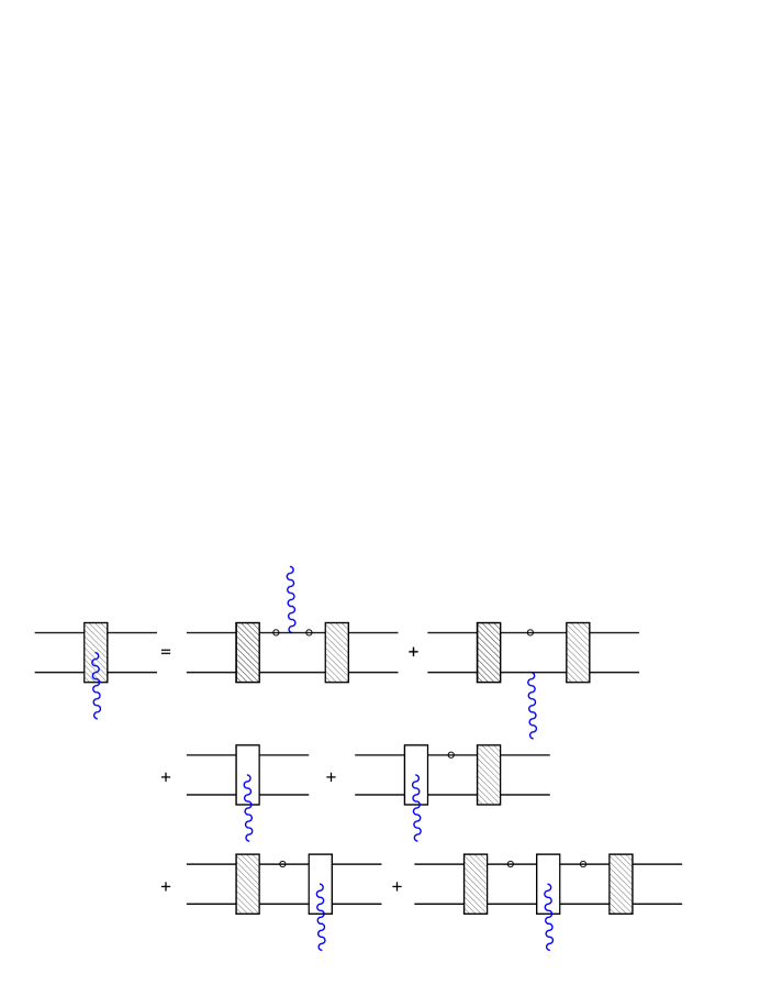
FIG. 12.: Feynman diagrams representing $\widetilde{J}^{\mu}_{\rm int}$. The open circles on particle line 1 are the difference propagator $\Delta G_{1}$, the shaded rectangles are the quasipotential $U$, and the open rectangles with photon attached are $\overline{J}^{\mu}_{ex}$.

$$\mathchoice{{\hbox{\boldmath$\displaystyle J$}}}{{\hbox{\boldmath$\textstyle J$}}}{{\hbox{\boldmath$\scriptstyle J$}}}{{\hbox{\boldmath$\scriptscriptstyle J$}}}^{\mu}_{\rm IA,eff}=\mathchoice{{\hbox{\boldmath$\displaystyle Q$}}}{{\hbox{\boldmath$\textstyle Q$}}}{{\hbox{\boldmath$\scriptstyle Q$}}}{{\hbox{\boldmath$\scriptscriptstyle Q$}}}\left(\begin{array}[]{cc}2J^{\mu}_{2}+j^{\mu}_{1}+j_{1}^{\mu\dagger}+j^{\mu}&j^{\mu}_{1}+j_{2}^{\mu\dagger}+j^{\mu}\\ j^{\mu}_{2}+j_{1}^{\mu\dagger}+j^{\mu}&2J^{\mu}_{1}+j^{\mu}_{2}+j_{2}^{\mu\dagger}+j^{\mu}\end{array}\right)\mathchoice{{\hbox{\boldmath$\displaystyle Q$}}}{{\hbox{\boldmath$\textstyle Q$}}}{{\hbox{\boldmath$\scriptstyle Q$}}}{{\hbox{\boldmath$\scriptscriptstyle Q$}}}\,,$$ (201)

where

$$j^{\mu}_{1}=-J^{\mu}_{1}\Delta G_{1}\overline{U}$$ (202)

$$j_{1}^{\mu\dagger}=-\overline{U}\Delta G_{1}J^{\mu}_{1}$$ (203)

$$j^{\mu}=-{\textstyle\frac{1}{2}}\,i\overline{U}\Bigl{[}\Delta G_{1}J_{1}^{\mu}\Delta G_{1}G_{2}+G_{2}J^{\mu}_{2}G_{2}\Delta G_{1}+(1\leftrightarrow 2)\Bigr{]}\overline{U}\,,$$ (204)

and $j_{2}$ is obtained from $j_{1}$ by substituting 2 for 1. Next, recall that $\zeta{\cal P}_{12}$ exchanges particles 1 and 2 (where $\zeta=\pm$ depending on statistics of the particles), and use the identities

$$\left|\psi_{2}\right>=\zeta{\cal P}_{12}\left|\psi_{1}\right>$$ (205)

$$\Delta g_{2}=\zeta{\cal P}_{12}\,\Delta g_{1}\,\zeta{\cal P}_{12}$$ (206)

$$\overline{U}=\zeta{\cal P}_{12}\,\overline{U}=\overline{U}\,\zeta{\cal P}_{12}=\zeta{\cal P}_{12}\,\overline{U}\,\zeta{\cal P}_{12}$$ (207)

$$J^{\mu}_{\rm IA}=\zeta{\cal P}_{12}\,J^{\mu}_{\rm IA}\,\zeta{\cal P}_{12}$$ (208)

$$\overline{J}^{\mu}_{\rm ex}=\zeta{\cal P}_{12}\,\overline{J}^{\mu}_{\rm ex}=\overline{J}^{\mu}_{\rm ex}\,\zeta{\cal P}_{12}=\zeta{\cal P}_{12}\,\overline{J}^{\mu}_{\rm ex}\,\zeta{\cal P}_{12}$$ (209)

to show that

$$\left<{\psi}_{2}\right|{J}^{\mu}_{1}\left|{\psi}_{2}\right>=\left<{\psi}_{1}\right|{J}^{\mu}_{2}\left|{\psi}_{1}\right>$$ (210)

$$\left<{\psi}_{1}\right|{j}^{\mu}_{1}\left|{\psi}_{1}\right>=\left<{\psi}_{1}\right|{j}^{\mu}_{1}\left|{\psi}_{2}\right>=\left<{\psi}_{2}\right|{j}^{\mu}_{2}\left|{\psi}_{1}\right>=\left<{\psi}_{2}\right|{j}^{\mu}_{2}\left|{\psi}_{2}\right>$$ (211)

$$\left<{\psi}_{1}\right|{j}^{\mu\dagger}_{1}\left|{\psi}_{1}\right>=\left<{\psi}_{2}\right|{j}^{\mu\dagger}_{1}\left|{\psi}_{1}\right>=\left<{\psi}_{1}\right|{j}^{\mu\dagger}_{2}\left|{\psi}_{2}\right>=\left<{\psi}_{2}\right|{j}^{\mu\dagger}_{2}\left|{\psi}_{2}\right>$$ (212)

$$\left<{\psi}_{1}\right|{j}^{\mu}\left|{\psi}_{1}\right>=\left<{\psi}_{1}\right|{j}^{\mu}\left|{\psi}_{2}\right>=\left<{\psi}_{2}\right|{j}^{\mu}\left|{\psi}_{1}\right>=\left<{\psi}_{2}\right|{j}^{\mu}\left|{\psi}_{2}\right>\,.$$ (213)

Hence

$$\left<\mathchoice{{\hbox{\boldmath$\displaystyle\psi$}}}{{\hbox{\boldmath$\textstyle\psi$}}}{{\hbox{\boldmath$\scriptstyle\psi$}}}{{\hbox{\boldmath$\scriptscriptstyle\psi$}}}\right|\mathchoice{{\hbox{\boldmath$\displaystyle J$}}}{{\hbox{\boldmath$\textstyle J$}}}{{\hbox{\boldmath$\scriptstyle J$}}}{{\hbox{\boldmath$\scriptscriptstyle J$}}}^{\mu}\left|\mathchoice{{\hbox{\boldmath$\displaystyle\psi$}}}{{\hbox{\boldmath$\textstyle\psi$}}}{{\hbox{\boldmath$\scriptstyle\psi$}}}{{\hbox{\boldmath$\scriptscriptstyle\psi$}}}\right> = {\textstyle\frac{1}{4}}\,\Bigl{[}\left<{\psi}_{1}\right|\mathchoice{{\hbox{\boldmath$\displaystyle J$}}}{{\hbox{\boldmath$\textstyle J$}}}{{\hbox{\boldmath$\scriptstyle J$}}}{{\hbox{\boldmath$\scriptscriptstyle J$}}}^{\mu}_{11}\left|{\psi}_{1}\right>+\left<{\psi}_{1}\right|\mathchoice{{\hbox{\boldmath$\displaystyle J$}}}{{\hbox{\boldmath$\textstyle J$}}}{{\hbox{\boldmath$\scriptstyle J$}}}{{\hbox{\boldmath$\scriptscriptstyle J$}}}^{\mu}_{12}\left|{\psi}_{2}\right>+\left<{\psi}_{2}\right|\mathchoice{{\hbox{\boldmath$\displaystyle J$}}}{{\hbox{\boldmath$\textstyle J$}}}{{\hbox{\boldmath$\scriptstyle J$}}}{{\hbox{\boldmath$\scriptscriptstyle J$}}}^{\mu}_{21}\left|{\psi}_{1}\right>+\left<{\psi}_{2}\right|\mathchoice{{\hbox{\boldmath$\displaystyle J$}}}{{\hbox{\boldmath$\textstyle J$}}}{{\hbox{\boldmath$\scriptstyle J$}}}{{\hbox{\boldmath$\scriptscriptstyle J$}}}^{\mu}_{22}\left|{\psi}_{2}\right>\Bigr{]}$$ (214)

$$= \left<\psi_{1}\right|\biggl{[}J^{\mu}_{2}-J^{\mu}_{1}G_{1}\overline{U}-\overline{U}G_{1}J^{\mu}_{1}-i\overline{U}\Delta G_{1}J^{\mu}_{1}\Delta G_{1}G_{2}\overline{U}$$ (216)

$$\qquad-i\overline{U}\Delta G_{1}G_{2}J^{\mu}_{2}G_{2}\overline{U}+\left(1-\overline{U}\Delta g_{1}\right)\overline{J}^{\mu}_{\rm ex}\left(1-\Delta g_{1}\overline{U}\right)\biggr{]}\left|\psi_{1}\right>.$$

Note that this is identical to (118), provided that the symmetrized two-body interaction is substituted for $U$, the symmetrized interaction current is substituted for $J^{\mu}_{\rm ex}$, and the masses and charges are set equal to each other. Hence we have show that Eq. (118) may be used either for identical or nonidentical particles.

B Final expressions for the currents

Now we will write explicit expressions for the matrix elements of the effective current between two bound states and between a bound initial state and a scattering final state. To facilitate this define an effective interaction current

$$\widetilde{J}^{\mu}_{\rm int}=-i\overline{U}\Delta G_{1}J^{\mu}_{1}\Delta G_{1}G_{2}\overline{U}-i\overline{U}\Delta G_{1}G_{2}J^{\mu}_{2}G_{2}\overline{U}+\left(1-\overline{U}\Delta g_{1}\right)\overline{J}^{\mu}_{ex}\left(1-\Delta g_{1}\overline{U}\right)\,.$$ (217)

This current is illustrated diagrammatically in Fig. 12.

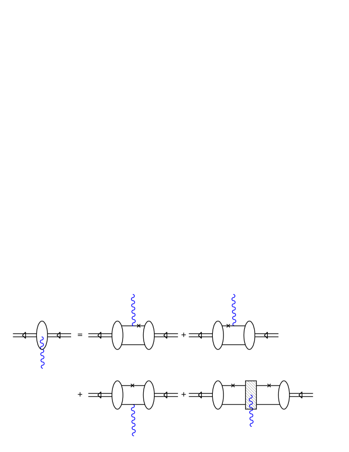
FIG. 13.: Feynman diagrams representing the matrix element of the effective current between bound states.

The matrix element of the effective current between bound states can then be written

$$\left<\mathchoice{{\hbox{\boldmath$\displaystyle\psi$}}}{{\hbox{\boldmath$\textstyle\psi$}}}{{\hbox{\boldmath$\scriptstyle\psi$}}}{{\hbox{\boldmath$\scriptscriptstyle\psi$}}}\right|\mathchoice{{\hbox{\boldmath$\displaystyle J$}}}{{\hbox{\boldmath$\textstyle J$}}}{{\hbox{\boldmath$\scriptstyle J$}}}{{\hbox{\boldmath$\scriptscriptstyle J$}}}^{\mu}\left|\mathchoice{{\hbox{\boldmath$\displaystyle\psi$}}}{{\hbox{\boldmath$\textstyle\psi$}}}{{\hbox{\boldmath$\scriptstyle\psi$}}}{{\hbox{\boldmath$\scriptscriptstyle\psi$}}}\right> = \left<\psi_{1}\right|\left[J^{\mu}_{2}-J^{\mu}_{1}G_{1}\overline{U}-\overline{U}G_{1}J^{\mu}_{1}+\widetilde{J}^{\mu}_{\rm int}\right]\left|\psi_{1}\right>$$ (218)

$$= \left<\psi_{1}\right|J^{\mu}_{2}\left|\psi_{1}\right>-\left<\psi_{1}\right|J^{\mu}_{1}G_{1}\overline{U}g_{1}\left|\Gamma_{1}\right>-\left<\Gamma_{1}\right|g_{1}\overline{U}G_{1}J^{\mu}_{1}\left|\psi_{1}\right>+\left<\psi_{1}\right|\widetilde{J}^{\mu}_{\rm int}\left|\psi_{1}\right>.$$ (219)

In numerical calculations it is often convenient to introduce an off-shell vertex function

$$\left|\Gamma\right>=-\overline{U}g_{i}\left|\Gamma_{i}\right>\,,$$ (220)

where $i=1,2$. This can be used to rewrite (219) as

$$\left<\mathchoice{{\hbox{\boldmath$\displaystyle\psi$}}}{{\hbox{\boldmath$\textstyle\psi$}}}{{\hbox{\boldmath$\scriptstyle\psi$}}}{{\hbox{\boldmath$\scriptscriptstyle\psi$}}}\right|\mathchoice{{\hbox{\boldmath$\displaystyle J$}}}{{\hbox{\boldmath$\textstyle J$}}}{{\hbox{\boldmath$\scriptstyle J$}}}{{\hbox{\boldmath$\scriptscriptstyle J$}}}^{\mu}\left|\mathchoice{{\hbox{\boldmath$\displaystyle\psi$}}}{{\hbox{\boldmath$\textstyle\psi$}}}{{\hbox{\boldmath$\scriptstyle\psi$}}}{{\hbox{\boldmath$\scriptscriptstyle\psi$}}}\right>=\left<\Gamma\right|G_{1}J^{\mu}_{1}\left|\psi_{1}\right>+\left<\psi_{1}\right|J^{\mu}_{1}G_{1}\left|\Gamma\right>+\left<\psi_{1}\right|J^{\mu}_{2}\left|\psi_{1}\right>+\left<\psi_{1}\right|\widetilde{J}^{\mu}_{\rm int}\left|\psi_{1}\right>.$$ (221)

The Feynman diagrams representing the elastic matrix element are shown in Fig. 13.

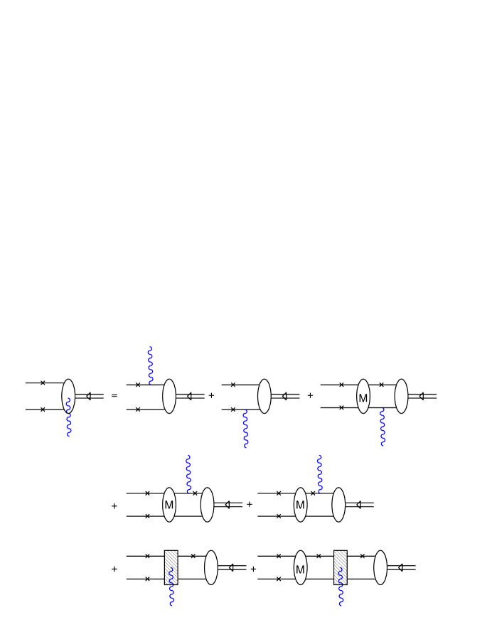
FIG. 14.: Feynman diagrams representing the matrix element of the effective current between a final scattering state and an initial bound state.

The matrix element of the effective current between a bound initial state and a scattering final state is

$$\left<\mathchoice{{\hbox{\boldmath$\displaystyle\psi$}}}{{\hbox{\boldmath$\textstyle\psi$}}}{{\hbox{\boldmath$\scriptstyle\psi$}}}{{\hbox{\boldmath$\scriptscriptstyle\psi$}}}^{(-)}\right|\mathchoice{{\hbox{\boldmath$\displaystyle J$}}}{{\hbox{\boldmath$\textstyle J$}}}{{\hbox{\boldmath$\scriptstyle J$}}}{{\hbox{\boldmath$\scriptscriptstyle J$}}}^{\mu}\left|\mathchoice{{\hbox{\boldmath$\displaystyle\psi$}}}{{\hbox{\boldmath$\textstyle\psi$}}}{{\hbox{\boldmath$\scriptstyle\psi$}}}{{\hbox{\boldmath$\scriptscriptstyle\psi$}}}\right> = \left<\mathchoice{{\hbox{\boldmath$\displaystyle p$}}}{{\hbox{\boldmath$\textstyle p$}}}{{\hbox{\boldmath$\scriptstyle p$}}}{{\hbox{\boldmath$\scriptscriptstyle p$}}}_{1},s_{1};\mathchoice{{\hbox{\boldmath$\displaystyle p$}}}{{\hbox{\boldmath$\textstyle p$}}}{{\hbox{\boldmath$\scriptstyle p$}}}{{\hbox{\boldmath$\scriptscriptstyle p$}}}_{2},s_{2}\right|{\cal A}_{2}(1-Mg_{1}){\cal Q}_{1}\left[J^{\mu}_{2}-J^{\mu}_{1}G_{1}\overline{U}-\overline{U}G_{1}J^{\mu}_{1}+\widetilde{J}^{\mu}_{\rm int}\right]\left|\psi_{1}\right>$$ (222)

Using the identities

$${\cal A}_{2}M=M$$ (223)

$${\cal A}_{2}\widetilde{J}^{\mu}_{\rm int}=\widetilde{J}^{\mu}_{\rm int}$$ (224)

$$\left<\mathchoice{{\hbox{\boldmath$\displaystyle p$}}}{{\hbox{\boldmath$\textstyle p$}}}{{\hbox{\boldmath$\scriptstyle p$}}}{{\hbox{\boldmath$\scriptscriptstyle p$}}}_{1},s_{1};\mathchoice{{\hbox{\boldmath$\displaystyle p$}}}{{\hbox{\boldmath$\textstyle p$}}}{{\hbox{\boldmath$\scriptstyle p$}}}{{\hbox{\boldmath$\scriptscriptstyle p$}}}_{2},s_{2}\right|{\cal A}_{2}\left(1-Mg_{1}\right){\cal Q}_{1}\overline{U}=\left<\mathchoice{{\hbox{\boldmath$\displaystyle p$}}}{{\hbox{\boldmath$\textstyle p$}}}{{\hbox{\boldmath$\scriptstyle p$}}}{{\hbox{\boldmath$\scriptscriptstyle p$}}}_{1},s_{1};\mathchoice{{\hbox{\boldmath$\displaystyle p$}}}{{\hbox{\boldmath$\textstyle p$}}}{{\hbox{\boldmath$\scriptstyle p$}}}{{\hbox{\boldmath$\scriptscriptstyle p$}}}_{2},s_{2}\right|M$$ (225)

$$\left<\mathchoice{{\hbox{\boldmath$\displaystyle p$}}}{{\hbox{\boldmath$\textstyle p$}}}{{\hbox{\boldmath$\scriptstyle p$}}}{{\hbox{\boldmath$\scriptscriptstyle p$}}}_{1},s_{1};\mathchoice{{\hbox{\boldmath$\displaystyle p$}}}{{\hbox{\boldmath$\textstyle p$}}}{{\hbox{\boldmath$\scriptstyle p$}}}{{\hbox{\boldmath$\scriptscriptstyle p$}}}_{2},s_{2}\right|{\cal A}_{2}\left(J^{\mu}_{2}-J^{\mu}_{1}G_{1}\overline{U}\right)\left|\psi_{1}\right>$$ (226)

$$\quad\quad=\left<\mathchoice{{\hbox{\boldmath$\displaystyle p$}}}{{\hbox{\boldmath$\textstyle p$}}}{{\hbox{\boldmath$\scriptstyle p$}}}{{\hbox{\boldmath$\scriptscriptstyle p$}}}_{1},s_{1};\mathchoice{{\hbox{\boldmath$\displaystyle p$}}}{{\hbox{\boldmath$\textstyle p$}}}{{\hbox{\boldmath$\scriptstyle p$}}}{{\hbox{\boldmath$\scriptscriptstyle p$}}}_{2},s_{2}\right|{\textstyle\frac{1}{2}}\Bigl{[}J^{\mu}_{2}G_{2}\left|\Gamma_{1}\right>+J^{\mu}_{1}G_{1}\left|\Gamma_{2}\right>+J^{\mu}_{2}G_{2}\left|\Gamma\right>+J^{\mu}_{1}G_{1}\left|\Gamma\right>\Bigr{]}$$ (227)

$$\quad\quad\quad\left<\mathchoice{{\hbox{\boldmath$\displaystyle p$}}}{{\hbox{\boldmath$\textstyle p$}}}{{\hbox{\boldmath$\scriptstyle p$}}}{{\hbox{\boldmath$\scriptscriptstyle p$}}}_{1},s_{1};\mathchoice{{\hbox{\boldmath$\displaystyle p$}}}{{\hbox{\boldmath$\textstyle p$}}}{{\hbox{\boldmath$\scriptstyle p$}}}{{\hbox{\boldmath$\scriptscriptstyle p$}}}_{2},s_{2}\right|\Bigl{[}J^{\mu}_{1}G_{1}\left|\Gamma_{2}\right>+J^{\mu}_{2}G_{2}\left|\Gamma_{1}\right>\Bigr{]}=\left<\mathchoice{{\hbox{\boldmath$\displaystyle p$}}}{{\hbox{\boldmath$\textstyle p$}}}{{\hbox{\boldmath$\scriptstyle p$}}}{{\hbox{\boldmath$\scriptscriptstyle p$}}}_{1},s_{1};\mathchoice{{\hbox{\boldmath$\displaystyle p$}}}{{\hbox{\boldmath$\textstyle p$}}}{{\hbox{\boldmath$\scriptstyle p$}}}{{\hbox{\boldmath$\scriptscriptstyle p$}}}_{2},s_{2}\right|\Bigl{[}J^{\mu}_{1}\left|\psi_{2}\right>+J^{\mu}_{2}\left|\psi_{1}\right>\Bigr{]}$$ (228)

where to get the last relation we employed (220), the current matrix element can be rewritten

$$\left<\mathchoice{{\hbox{\boldmath$\displaystyle\psi$}}}{{\hbox{\boldmath$\textstyle\psi$}}}{{\hbox{\boldmath$\scriptstyle\psi$}}}{{\hbox{\boldmath$\scriptscriptstyle\psi$}}}^{(-)}\bigl{|}\mathchoice{{\hbox{\boldmath$\displaystyle J$}}}{{\hbox{\boldmath$\textstyle J$}}}{{\hbox{\boldmath$\scriptstyle J$}}}{{\hbox{\boldmath$\scriptscriptstyle J$}}}^{\mu}\bigr{|}\mathchoice{{\hbox{\boldmath$\displaystyle\psi$}}}{{\hbox{\boldmath$\textstyle\psi$}}}{{\hbox{\boldmath$\scriptstyle\psi$}}}{{\hbox{\boldmath$\scriptscriptstyle\psi$}}}\right> = \Bigl{<}\mathchoice{{\hbox{\boldmath$\displaystyle p$}}}{{\hbox{\boldmath$\textstyle p$}}}{{\hbox{\boldmath$\scriptstyle p$}}}{{\hbox{\boldmath$\scriptscriptstyle p$}}}_{1},s_{1};\mathchoice{{\hbox{\boldmath$\displaystyle p$}}}{{\hbox{\boldmath$\textstyle p$}}}{{\hbox{\boldmath$\scriptstyle p$}}}{{\hbox{\boldmath$\scriptscriptstyle p$}}}_{2},s_{2}\Bigl{|}\biggl{[}J^{\mu}_{1}\left|\psi_{2}\right>+J^{\mu}_{2}\left|\psi_{1}\right>-Mg_{1}J^{\mu}_{2}\left|\psi_{1}\right>-MG_{1}J^{\mu}_{1}\left|\psi_{1}\right>$$ (230)

$$\qquad\qquad\quad+Mg_{1}Q_{1}J^{\mu}_{1}G_{1}\overline{U}\left|\psi_{1}\right>+(1-Mg_{1}Q_{1})\widetilde{J}^{\mu}_{\rm int}\left|\psi_{1}\right>\biggr{]}$$

$$= \Bigl{<}\mathchoice{{\hbox{\boldmath$\displaystyle p$}}}{{\hbox{\boldmath$\textstyle p$}}}{{\hbox{\boldmath$\scriptstyle p$}}}{{\hbox{\boldmath$\scriptscriptstyle p$}}}_{1},s_{1};\mathchoice{{\hbox{\boldmath$\displaystyle p$}}}{{\hbox{\boldmath$\textstyle p$}}}{{\hbox{\boldmath$\scriptstyle p$}}}{{\hbox{\boldmath$\scriptscriptstyle p$}}}_{2},s_{2}\Bigl{|}\biggl{[}J^{\mu}_{1}\left|\psi_{2}\right>+J^{\mu}_{2}\left|\psi_{1}\right>-MG_{2}J^{\mu}_{2}\left|\psi_{1}\right>-MG_{1}J^{\mu}_{1}\left|\psi_{1}\right>$$ (232)

$$\qquad\qquad\quad-MQ_{1}J^{\mu}_{1}G_{1}G_{2}\left|\Gamma\right>+(1-MQ_{1}G_{2})\widetilde{J}^{\mu}_{\rm int}\left|\psi_{1}\right>\biggr{]}\,.$$

The Feynman diagrams representing the inelastic matrix element are shown in Fig. 14.

C Comparison to Bethe-Salpeter matrix elements

Let us now compare the matrix elements derived above with those of the Bethe-Salpeter description. First, consider the elastic Bethe-Salpeter matrix element

$$\left<\psi\right|J^{\mu}\left|\psi\right>_{\rm BS} = \left<\Gamma\right|G_{\rm BS}\left(iJ^{\mu}_{1}G^{-1}_{2}+iJ^{\mu}_{2}G^{-1}_{1}+\overline{J}^{\mu}_{\rm ex}\right)G_{\rm BS}\left|\Gamma\right>$$ (233)

$$= \left<\Gamma\right|-iG_{1}J^{\mu}_{1}G_{1}G_{2}-iG_{1}G_{2}J^{\mu}_{2}G_{2}-G_{1}G_{2}\overline{J}^{\mu}_{\rm ex}G_{1}G_{2}\left|\Gamma\right>\,.$$ (234)

With the help of simple identities obtained from Eqs. (48) and (99)

$$-iG_{1}J^{\mu}_{1}G_{1}G_{2} = {\cal Q}_{1}J^{\mu}_{1}G_{1}G_{2}+G_{1}J^{\mu}_{1}{\cal Q}_{1}G_{2}-i\Delta G_{1}J^{\mu}_{1}\Delta G_{1}G_{2}\,,$$ (235)

$$-iG_{1}G_{2}J^{\mu}_{2}G_{2} = {\cal Q}_{1}G_{2}J^{\mu}_{2}G_{2}-i\Delta G_{1}G_{2}J^{\mu}_{2}G_{2}\,,$$ (236)

$$-G_{1}G_{2}\overline{J}^{\mu}_{\rm ex}G_{1}G_{2} = ({\cal Q}_{1}-i\Delta G_{1})G_{2}\overline{J}^{\mu}_{\rm ex}G_{2}({\cal Q}_{1}-i\Delta G_{1})\,,$$ (237)

relation (220), and the conventions (61) and (62), we can rewrite (234) as

$$\left<\psi\right|J^{\mu}\left|\psi\right>_{\rm BS}= \left<\Gamma\right|Q_{1}G_{2}\left[J^{\mu}_{2}-J^{\mu}_{1}G_{1}\overline{U}-\overline{U}G_{1}J^{\mu}_{1}+\widetilde{J}^{\mu}_{\rm int}\right]Q_{1}G_{2}\left|\Gamma\right>$$ (238)

$$= \left<\psi_{1}\right|\left[J^{\mu}_{2}-J^{\mu}_{1}G_{1}\overline{U}-\overline{U}G_{1}J^{\mu}_{1}+\widetilde{J}^{\mu}_{\rm int}\right]\left|\psi_{1}\right>\,,$$ (239)

with $\widetilde{J}^{\mu}_{\rm int}$ defined by (217). We have demonstrated again that our spectator matrix element (219) exactly equals Bethe-Salpeter one (234). Of course, this should be so by construction. Still, the derivation of this section gives a useful shortcut to the correct spectator matrix element. It also illustrates how the current $J^{\mu}_{2}-J^{\mu}_{1}G_{1}\overline{U}-\overline{U}G_{1}J^{\mu}_{1}$ in (219) and (239) follows from the Bethe-Salpeter matrix element if one puts the first particle on-shell, i.e., if one keeps only the first term in Eq. (142) for the quasipotential (for consistency we should replace $\overline{U}\to\overline{V}$, which also holds when all terms with $\Delta G_{1}$ are omitted). The last part of the effective current $\widetilde{J}^{\mu}_{\rm int}$ then gathers all higher order effects. A very similar consideration can be applied to the break-up matrix element (222). One finds that the parts of the matrix element with loops can again be related by identities (237), while the loopless parts, i.e., an IA contributions without a final-state interaction, are identical for both approaches.

V Charge conservation

In this section we show that the total charge of a bound state is equal to the sum of the charges of its constituents, $e_{1}+e_{2}$, and discuss how this result emerges automatically in the Bethe-Salpeter and spectator formalisms. In this discussion we will assume for definiteness that the two particles are nonidentical, but our results will hold for identical particles also since the current operator in the latter case is obtained by symmetrization of the former one.

First recall that taking the $q\to 0$ limit of the one-body Ward-Takahashi (WT) identity, Eq. (27), implies that the one-body currents satisfy

$$J^{\mu}_{i}(0)=-e_{i}\frac{dG_{i}^{-1}(p_{i})}{dp_{i,\mu}}\,.$$ (240)

This relation will be used in both formalisms.

Next consider the two-body WT identity, Eq. (28), in the context of the BS formalism. It is well known [13] that the contribution to the charge operator which comes from the exchange current can be uniquely determined by taking the $q\to 0$ limit of (28). The derivation of this result was discussed in great detail by Bentz [14], and we only review it briefly here. Since the overall four-momentum is conserved, the kernel is a function of only three independent four-momenta, which can be chosen to be either $P$, $p$, and $p^{\prime}$, or $P$, $p_{1}$, and $p^{\prime}_{1}$. Depending on how we choose the independent momenta, the $q\to 0$ limit of Eq. (28) gives

$$J^{\mu}_{\rm ex}(0) = -(e_{1}+e_{2})\,\frac{\partial V(p^{\prime},p,P)}{\partial P_{\mu}}-\frac{(e_{1}-e_{2})}{2}\,\left[\frac{\partial V(p^{\prime},p,P)}{\partial p^{\prime}_{\mu}}+\frac{\partial V(p^{\prime},p,P)}{\partial p_{\mu}}\right]$$ (241)

$$= -(e_{1}+e_{2})\,\frac{\partial V(p^{\prime}_{1},p_{1},P)}{\partial P_{\mu}}-e_{1}\,\left[\frac{\partial V(p_{1}^{\prime},p_{1},P)}{\partial p^{\prime}_{1,\mu}}+\frac{\partial V(p^{\prime}_{1},p_{1},P)}{\partial p_{1,\mu}}\right]\,,$$ (242)

where in (241) the partial derivative with respect $P_{\mu}$ implies that the independent vectors $p_{\mu}$ and $p^{\prime}_{\mu}$ are held constant, while in (242) the partial derivative with respect $P_{\mu}$ implies that the independent vectors $p_{1,\mu}$ and $p^{\prime}_{1,\mu}$ are held constant. Similarly,

$$-i\frac{dG_{1}^{-1}(p_{1})}{dp_{1,\mu}}G_{2}^{-1}(p_{2})= -\frac{\partial G_{\rm BS}^{-1}(p,P)}{\partial P_{\mu}}-{1\over 2}\frac{\partial G_{\rm BS}^{-1}(p,P)}{\partial p_{\mu}}$$ (243)

$$= -\frac{\partial G_{\rm BS}^{-1}(p_{1},P)}{\partial P_{\mu}}-\frac{\partial G_{\rm BS}^{-1}(p_{1},P)}{\partial p_{1,\mu}}$$ (244)

and

$$-iG_{1}^{-1}(p_{1})\frac{dG_{2}^{-1}(p_{2})}{dp_{2,\mu}}= -\frac{\partial G_{\rm BS}^{-1}(p,P)}{\partial P_{\mu}}+{1\over 2}\frac{\partial G_{\rm BS}^{-1}(p,P)}{\partial p_{\mu}}$$ (245)

$$= -\frac{\partial G_{\rm BS}^{-1}(p_{1},P)}{\partial P_{\mu}}\,.$$ (246)

The correct forms of these equations depend on our choice of independent vectors. In the BS case either of the forms can be used since there are no additional constraints on the vectors, but in the spectator case with particle 1 on-shell we must use (242), (244), and (246) because $p_{2}$ will explicitly depend on $P$ in cases when $p_{1}$ is constrained.

We use (241), (244), and (246) to evaluate the bound state matrix element of the charge operator in the BS formalism

$$\left<\psi\right|J^{\mu}(0)\left|\psi\right> = -\left<\psi\right|e_{1}\,i\frac{dG_{1}^{-1}(p_{1})}{dp_{1,\mu}}G_{2}^{-1}(p_{2})+e_{2}\,iG_{1}^{-1}(p_{1})\frac{dG_{2}^{-1}(p_{2})}{dp_{2,\mu}}-J^{\mu}_{\rm ex}(0)\left|\psi\right>$$ (247)

$$= -\left<\psi\right|(e_{1}+e_{2})\,\biggl{(}\frac{\partial G_{\rm BS}^{-1}(p,P)}{\partial P_{\mu}}+\frac{\partial V(p^{\prime},p,P)}{\partial P_{\mu}}\biggr{)}$$ (249)

$$\quad+\frac{e_{1}-e_{2}}{2}\biggl{(}\frac{\partial G_{\rm BS}^{-1}(p,P)}{\partial p_{\mu}}+\frac{\partial V(p^{\prime},p,P)}{\partial p^{\prime}_{\mu}}+\frac{\partial V(p^{\prime},p,P)}{\partial p_{\mu}}\biggr{)}\left|\psi\right>$$

$$= (e_{1}+e_{2})\,2P^{\mu}\,,$$ (250)

where the normalization condition for the BS vertex function [6, 13] was used in the last step to simplify the $(e_{1}+e_{2})$ terms, and the cancellation of the $(e_{1}-e_{2})$ terms follows from integrating $\partial G^{-1}_{\rm BS}/\partial p_{\mu}$ by parts and using the bound state BS equation (24). The final form of (250) shows that the charge is conserved.

Now we turn to the spectator formalism with the effective current given in Eq. (116). We begin by pointing out that, unlike in the Bethe-Salpeter case, one cannot obtain $J^{\mu}_{11}(0)$ from the corresponding Ward-Takahashi identity (130). For nonidentical particles the clear indication of this fact is that the charge of the first particle (which can be completely arbitrary) is absent from the WT relation (130) and any current determined from this relation would therefore depend on $e_{2}$ only, which is certainly not correct. The reason for this was alluded to in Sec. III: the condition restricting the first particle to its mass shell leads to an effective current in which the terms proportional to the charge of particle 1 are purely transverse. There can be also transverse currents in the BS case, but they are of the form $a_{\mu\nu}q^{\nu}$, with $a_{\mu\nu}$ antisymmetric and nonsingular for $q\to 0$, and hence they vanish in this limit, and all parts of the current contributing to the charge can be recovered from the WT identity (see Ref. [14]). In the spectator formalism those parts of the current which are transverse by virtue of the on-shell condition do not vanish in the $q\to 0$ limit. Therefore, the effective current in $q\to 0$ limit cannot be fully recovered from the WT identity and has to be obtained by taking the limit explicitly.

The effective spectator current for zero photon momentum follows from Eqs. (116) and (242)

$$J^{\mu}_{11}(0) = {\cal Q}_{1}\biggl{\{}-e_{2}\frac{dG_{2}^{-1}}{dp_{2,\mu}}-\left[J_{1}^{\mu}G_{1}U+UG_{1}J_{1}^{\mu}\right]_{q\,\to\,0}\,+\left(1-U\Delta g_{1}\right)J^{\mu}_{\rm ex}(0)\left(1-\Delta g_{1}U\right)$$ (252)

$$+\left[ie_{1}\,U\Delta G_{1}\frac{dG_{1}^{-1}}{dp^{\prime\prime}_{1,\mu}}\,\Delta G_{1}G_{2}U+ie_{2}\,U\Delta G_{1}G_{2}\frac{dG_{2}^{-1}}{dp^{\prime\prime}_{2,\mu}}\,G_{2}U\right]\,\biggr{\}}{\cal Q}_{1}\,.$$

The first term in the last line of this equation can be reduced if we use rules (94) and (96) and integrate by parts twice (noting that $p_{1}$ is unconstrained in this loop and that $P$ is to be held constant)

$$ie_{1}U\Delta G_{1}\frac{dG_{1}^{-1}}{dp^{\prime\prime}_{1,\mu}}\,\Delta G_{1}G_{2}U= -ie_{1}\frac{\partial{U}(p_{1}^{\prime},p_{1}^{\prime\prime},P)}{\partial p^{\prime\prime}_{1,\mu}}\Delta G_{1}G_{2}U-ie_{1}U\Delta G_{1}G_{2}\frac{\partial{U}(p_{1}^{\prime\prime},p_{1},P)}{\partial p^{\prime\prime}_{1,\mu}}$$ (254)

$$-2ie_{1}U\frac{\partial\Delta G_{1}}{\partial p^{\prime\prime}_{1,\mu}}G_{2}U-ie_{1}U\Delta G_{1}\frac{\partial G_{2}}{\partial p^{\prime\prime}_{1,\mu}}U$$

$$= e_{1}U\frac{\partial\Delta g_{1}}{\partial p^{\prime\prime}_{1,\mu}}U+ie_{1}U\Delta G_{1}\frac{\partial G_{2}}{\partial p^{\prime\prime}_{1,\mu}}U\,,$$ (255)

where here and below $p^{\prime}_{1}$ and $p_{1}$ are the four-momenta of particle 1 after and before the interaction, respectively, and $p^{\prime\prime}_{1}$ denotes the momenta of the loop integration implied by the product $U\dots U$. Using

$$G_{2}\,\frac{dG_{2}^{-1}(p_{2})}{dp_{2,\mu}}\,G_{2}=\frac{\partial G_{2}(P-p_{1})}{\partial p_{1,\mu}}\,,$$ (256)

the second term in the last line of Eq. (252) becomes

$$ie_{2}U\Delta G_{1}G_{2}\frac{dG_{2}^{-1}}{dp^{\prime\prime}_{2,\mu}}\,G_{2}U=ie_{2}U\Delta G_{1}\frac{\partial G_{2}}{\partial p^{\prime\prime}_{1,\mu}}U\,.$$ (257)

The term with the exchange current $J^{\mu}_{\rm ex}(0)$ is simplified with the help of

$$\frac{\partial U}{\partial p^{\prime}_{1,\mu}} = \frac{\partial V}{\partial p^{\prime}_{1,\mu}}(1-\Delta g_{1}\,U)\,,$$ (258)

$$\frac{\partial U}{\partial p_{1,\mu}} = (1-U\,\Delta g_{1})\frac{\partial V}{\partial p_{1,\mu}}\,.$$ (259)

These relations are obtained by differentiating the corresponding off-shell quasipotential equations and using the fact that the structure of the integral equations insures that the only dependence on the final momentum $p^{\prime}_{1}$ in (258), or on the initial momentum $p_{1}$ in (259), is found in the kernel $V$. A similar argument gives

$$\frac{\partial U}{\partial P_{\mu}}=\frac{\partial V}{\partial P_{\mu}}(1-\Delta g_{1}\,U)-V\frac{\partial(\Delta g_{1}U)}{\partial P_{\mu}}$$ (260)

and hence

$$\left(1-U\Delta g_{1}\right)\frac{\partial{V}}{\partial P_{\mu}}\left(1-\Delta g_{1}U\right)= \frac{\partial U}{\partial P_{\mu}}-U\Delta g_{1}\frac{\partial U}{\partial P_{\mu}}+U\frac{\partial(\Delta g_{1}U)}{\partial P_{\mu}}$$ (261)

$$= \frac{\partial U}{\partial P_{\mu}}+U\frac{\partial\Delta g_{1}}{\partial P_{\mu}}U\,.$$ (262)

Hence using (242), (258), (259), and (262) gives

$$\left(1-U\Delta g_{1}\right) J^{\mu}_{\rm ex} (0)\left(1-\Delta g_{1}U\right)$$ (263)

$$= -(e_{1}+e_{2})\,\left[\frac{\partial U}{\partial P_{\mu}}+U\frac{\partial\Delta g_{1}}{\partial P_{\mu}}U\right]-e_{1}\,\left[\frac{\partial{U}(p_{1}^{\prime},p_{1},P)}{\partial p^{\prime}_{1,\mu}}+\frac{\partial{U}(p_{1}^{\prime},p_{1},P)}{\partial p_{1,\mu}}\right]$$ (265)

$$+e_{1}\,\left[U\Delta g_{1}\frac{\partial{U}(p_{1}^{\prime\prime},p_{1},P)}{\partial p^{\prime\prime}_{1,\mu}}+\frac{\partial{U}(p_{1}^{\prime},p_{1}^{\prime\prime},P)}{\partial p^{\prime\prime}_{1,\mu}}\Delta g_{1}U\right]$$

$$= -(e_{1}+e_{2})\,\left[\frac{\partial U}{\partial P_{\mu}}+U\frac{\partial\Delta g_{1}}{\partial P_{\mu}}U\right]-e_{1}\,\left[\frac{\partial{U}}{\partial p^{\prime}_{1,\mu}}+\frac{\partial{U}}{\partial p_{1,\mu}}+U\frac{\partial\Delta g_{1}}{\partial p^{\prime\prime}_{1,\mu}}U\right]\,,$$ (266)

Since $p^{\prime\prime}_{1}$ is off-shell in the integration loop, we could integrate by parts to simplify the last line of (265).

Making these substitutions and combining terms permits us to simplify Eq. (252)

$$J^{\mu}_{11}(0)=Q_{1}\biggl{\{} -e_{2}\frac{\partial G_{2}^{-1}}{\partial P_{\mu}}-\left[J_{1}^{\mu}G_{1}U+UG_{1}J_{1}^{\mu}\right]_{q\,\to\,0}-(e_{1}+e_{2})\,\frac{\partial U}{\partial P_{\mu}}$$ (269)

$$-e_{1}\,\left(\frac{\partial{U}(p_{1}^{\prime},p_{1},P)}{\partial p^{\prime}_{1,\mu}}+\frac{\partial{U}(p_{1}^{\prime},p_{1},P)}{\partial p_{1,\mu}}\right)$$

$$+(e_{1}+e_{2})\,U\,\left[i\Delta G_{1}\frac{\partial G_{2}}{\partial p^{\prime\prime}_{1,\mu}}-\frac{\partial\Delta g_{1}}{\partial P_{\mu}}\right]\,U\,\biggr{\}}Q_{1}\,.$$

Recall that partial derivative with respect to $P$ holds $p_{1}$ constant, and hence

$${\partial\Delta g_{1}(p_{1},P)\over\partial P_{\mu}}=-i\Delta G_{1}(p_{1}){\partial G_{2}(P-p_{1})\over\partial P_{\mu}}=i\Delta G_{1}(p_{1}){\partial G_{2}(P-p_{1})\over\partial p_{1,\mu}}\,,$$ (270)

so the last line proportional to $U^{2}$ in (269) cancels. The remaining terms will be now shown to be proportional to the normalization condition. Let us point out that exactly such terms (with $U\to V$) would appear if only the leading order quasipotential with corresponding currents are considered.

To simplify (269) one has to reduce the term $\left[J_{1}^{\mu}G_{1}U+UG_{1}J_{1}^{\mu}\right]_{q\,\to\,0}$. It must be treated carefully as each term is singular as $q\,\to\,0$, but, as discussed in Ref [6], the singularities cancel in the sum. Following the argument developed in Ref. [6], using the notation $\hat{p}_{1}$ and $\hat{p}^{\prime}_{1}$ to indicate those cases where the four-momenta of particle 1 are restricted to their mass shell, and exploiting the bound state equation (73) gives

$$-\left<\Gamma_{1}\right| G_{2}\bigl{[}J_{1}^{\mu}G_{1}U+UG_{1}J_{1}^{\mu}\bigr{]}_{q\,\to\,0}\,G_{2}\left|\Gamma_{1}\right>$$ (280)

$$=\left<\Gamma_{1}\right|G_{2}\left[U_{11}G_{2}J_{1}^{\mu}G_{1}U+UG_{1}J_{1}^{\mu}G_{2}U_{11}\right]G_{2}\left|\Gamma_{1}\right>_{q\,\to\,0}$$

$$\simeq-{e_{1}\over q_{\mu}}\left<\Gamma_{1}\right|G_{2}\biggl{\{}U_{11}(\hat{p}^{\prime}_{1},\hat{p}^{\prime\prime}_{1},P+q)\left[G_{1}^{-1}(\hat{p}^{\prime\prime}_{1})-G_{1}^{-1}(\hat{p}^{\prime\prime}_{1}-q)\right]G_{1}(\hat{p}^{\prime\prime}_{1}-q)$$

$$\qquad\qquad\times G_{2}(P-\hat{p}^{\prime\prime}_{1}+q)U(\hat{p}^{\prime\prime}_{1}-q,\hat{p}_{1},P)+U(\hat{p}^{\prime}_{1},\hat{p}^{\prime\prime}_{1}+q,P+q)G_{2}(P-\hat{p}^{\prime\prime}_{1})$$

$$\qquad\qquad\times G_{1}(\hat{p}^{\prime\prime}_{1}+q)\left[G_{1}^{-1}(\hat{p}^{\prime\prime}_{1}+q)-G_{1}^{-1}(\hat{p}^{\prime\prime}_{1})\right]U_{11}(\hat{p}^{\prime\prime}_{1},\hat{p}_{1},P)\biggr{\}}G_{2}\left|\Gamma_{1}\right>_{q\,\to\,0}$$

$$={e_{1}\over q_{\mu}}\left<\Gamma_{1}\right|G_{2}\biggl{\{}U_{11}(\hat{p}^{\prime}_{1},\hat{p}^{\prime\prime}_{1},P+q)G_{2}(P-\hat{p}^{\prime\prime}_{1}+q)U(\hat{p}^{\prime\prime}_{1}-q,\hat{p}_{1},P)$$

$$\qquad\qquad-U(\hat{p}^{\prime}_{1},{p}^{\prime\prime}_{1}+q,P+q)G_{2}(P-\hat{p}^{\prime\prime}_{1})U_{11}(\hat{p}^{\prime\prime}_{1},\hat{p}_{1},P)\biggr{\}}G_{2}\left|\Gamma_{1}\right>_{q\,\to\,0}$$

$$=e_{1}\,\left<\Gamma_{1}\right|G_{2}\biggl{(}U_{11}{\partial G_{2}\over\partial P_{\mu}}U_{11}-{\partial U\over\partial\hat{p}^{\prime\prime}_{1,\mu}}G_{2}U_{11}-U_{11}G_{2}{\partial U\over\partial\hat{p}^{\prime\prime}_{1,\mu}}\biggr{)}G_{2}\left|\Gamma_{1}\right>$$

$$=e_{1}\,\left<\Gamma_{1}\right|{\partial G_{2}(P-\hat{p}_{1})\over\partial P_{\mu}}$$

$$\qquad\qquad+G_{2}(P-\hat{p}^{\prime}_{1})\,\left(\frac{\partial U(\hat{p}^{\prime}_{1},\hat{p}_{1},P)}{\partial\hat{p}^{\prime}_{1,\mu}}+\frac{\partial U(\hat{p}^{\prime}_{1},\hat{p}_{1},P)}{\partial\hat{p}_{1,\mu}}\right)\,G_{2}(P-\hat{p}_{1})\,\left|\Gamma_{1}\right>\,,$$

where, in going from the second to the third step we used $G_{1}^{-1}Q_{1}=0$ for the on-shell momentum $\hat{p}^{\prime\prime}_{1}$, and in the last step we used the bound state equation to remove the factors of $G_{2}U$ whenever possible. When simplifying (280) it is important to choose the dummy integration momentum $p^{\prime\prime}_{1}$ so that the on-shell condition does not depend on the photon momentum $q$. Finally, substituting this result into (269) gives

$$J^{\mu}_{11}(0)=(e_{1}+e_{2})\,Q_{1}\left\{G_{2}^{-1}\frac{\partial G_{2}}{\partial P_{\mu}}G_{2}^{-1}-\frac{\partial U}{\partial P_{\mu}}\right\}Q_{1}\,,$$ (281)

and the elastic matrix element of the effective spectator current at $q=0$ becomes

$$\left<\psi_{1}\right|J^{\mu}_{11}(0)\left|\psi_{1}\right>= \left<\Gamma_{1}\right|G_{2}J^{\mu}_{11}(0)G_{2}\left|\Gamma_{1}\right>$$ (282)

$$= (e_{1}+e_{2})\left<\Gamma_{1}\right|\left(\frac{\partial G_{2}(P-\hat{p}_{1})}{\partial P_{\mu}}\right.$$ (284)

$$\left.-G_{2}(P-\hat{p}^{\prime}_{1})\,\frac{\partial U(\hat{p}^{\prime}_{1},\hat{p}_{1},P)}{\partial P_{\mu}}\,G_{2}(P-\hat{p}_{1})\,\right)\left|\Gamma_{1}\right>\,.$$

However, the normalization condition for the spectator vertex function is just

$$\left<\Gamma_{1}\right|\left(\frac{\partial G_{2}(P-\hat{p}_{1})}{\partial P_{\mu}}-G_{2}(P-\hat{p}^{\prime}_{1})\,\frac{\partial U(\hat{p}^{\prime}_{1},\hat{p}_{1},P)}{\partial P_{\mu}}\,G_{2}(P-\hat{p}_{1})\,\right)\left|\Gamma_{1}\right>=2P^{\mu}\,.$$ (285)

This was discussed in great detail in [6], where it was derived from the nonlinear form of the spectator equation without reference to the e.m. current (in that reference the spectator kernel was denoted by $V$, but the derivation did not specify the kernel in any way and holds equally well for the kernel $U$). Obviously the relations (284) and (285) are consistent with

$$\left<\Gamma_{1}\right|G_{2}J^{\mu}_{11}(0)G_{2}\left|\Gamma_{1}\right>=(e_{1}+e_{2})\,2P^{\mu}\,,$$ (286)

which is the statement that the charge of the bound state is $e_{1}+e_{2}$, completing our proof.

Our derivation is valid for any interaction $V$ and the corresponding quasipotential $U$ (e.g., also for phenomenological ones, such as a separable interaction). It is only necessary to have an interaction current at the Bethe-Salpeter level consistent with the one body current, so that the total BS current is conserved. Furthermore, since we have not specified the spins of the constituents or the bound state in our derivation, it should apply for arbitrary spins.

VI Truncation

To this point, no approximations have been made in constructing either the n-point functions or the effective current operators. In particular, the equivalence between the Gross equation and its quasipotential and the Bethe-Salpeter equation is exact only if the Bethe-Salpeter kernel $V$ and the spectator kernel $U$ are related by Eq. (53). This means that if one of the kernels is truncated to some finite order, the other must involve terms of all orders. In practice, both kernels are generally truncated to some finite order and the two formalisms do not give identical results. The usual approximation is to keep only the one-boson-exchange-contribution, either for $V^{(1)}$ or $U^{(1)}$. The problem is then to verify that the various relations leading to conserved current matrix elements are maintained in the presence of the truncation.

First assume that we have some Bethe-Salpeter kernel ${V}\rightarrow\lambda{V}$ and the associated current $J^{\mu}\rightarrow J^{\mu}_{\rm IA}+\lambda{J}^{\mu}_{\rm ex}$ where the interaction current and the interaction satisfy the Ward-Takahashi identity (28). [In this section we will again limit the discussion to nonidentical particles.]  Here the parameter $\lambda$ has been introduced to assist in the counting of occurrences of the interaction ${V}$ and the associated exchange current $J^{\mu}_{\rm ex}$ and will eventually be set to unity in all calculations. From (53) it is clear that the quasipotential can be written as a series in $\lambda$ as

$${U}=\sum_{N=1}^{\infty}\lambda^{N}{U}^{(N)}$$ (287)

Substituting this into (53) and collecting the coefficients of the various powers of $\lambda$, we can identify the quasipotential of the $N$-th rank ${U}^{(N)}$ as

$${U}^{(1)} = {V}\,,$$ (288)

$${U}^{(N)} = -{V}\Delta g_{1}{U}^{(N-1)}\,,\quad N>1\,.$$ (289)

Similarly, using (112) implies that the effective current can also be expanded

$$J^{\mu}_{11}=\sum_{N=1}^{\infty}\lambda^{N}J^{(N)\mu}_{11}$$ (290)

where the $N$-th rank contributions to the effective current are $J^{(N)\mu}_{11}=J^{(N)\mu}_{\rm IA,eff}+J^{(N)\mu}_{\rm ex,eff}$. For $J^{(N)\mu}_{\rm IA,eff}$ these contributions are

$$J^{(0)\mu}_{\rm IA,eff} = {\cal Q}_{1}J^{\mu}_{\rm IA}{\cal Q}_{1}\,,$$ (291)

$$J^{(1)\mu}_{\rm IA,eff} = -{\cal Q}_{1}\left({U}^{(1)}\Delta g_{1}J^{\mu}_{\rm IA}+J^{\mu}_{\rm IA}\Delta g_{1}{U}^{(1)}\right){\cal Q}_{1}\,,$$ (292)

$$J^{(N)\mu}_{\rm IA,eff} = -{\cal Q}_{1}\left({U}^{(N)}\Delta g_{1}J^{\mu}_{IA}+J^{\mu}_{IA}\Delta g_{1}{U}^{(N)}-\sum^{N-1}_{M=1}{U}^{(N-M)}\Delta g_{1}J^{\mu}_{IA}\Delta g_{1}{U}^{(M)}\right){\cal Q}_{1}\,,$$ (294)

$$\qquad\qquad\qquad\qquad\qquad\qquad\qquad\qquad\qquad\qquad\qquad\qquad{\rm if}\quad N>1\,,$$

and

$$J^{(0)\mu}_{\rm ex,eff} = 0,$$ (295)

$$J^{(1)\mu}_{\rm ex,eff} = {\cal Q}_{1}J^{\mu}_{\rm ex}{\cal Q}_{1},$$ (296)

$$J^{(2)\mu}_{\rm ex,eff} = -{\cal Q}_{1}\left({U}^{(1)}\Delta g_{1}J^{\mu}_{\rm ex}+J^{\mu}_{ex}\Delta g_{1}{U}^{(1)}\right){\cal Q}_{1},$$ (297)

$$J^{(N)\mu}_{\rm ex,eff} = -{\cal Q}_{1}\left({U}^{(N-1)}\Delta g_{1}J^{\mu}_{\rm ex}+J^{\mu}_{ex}\Delta g_{1}{U}^{(N-1)}-\sum^{N-2}_{M=1}{U}^{(N-M-1)}\Delta g_{1}J^{\mu}_{\rm ex}\Delta g_{1}{U}^{(M)}\right){\cal Q}_{1}\,,$$ (299)

$$\qquad\qquad\qquad\qquad\qquad\qquad\qquad\qquad\qquad\qquad\qquad\qquad{\rm if}\quad N>2\,.$$

At the lowest rank $N=0$ the particles do not interact and only disconnected diagrams [which are not fully described by the current (112)] occur. To get a nontrivial description of interacting particles and their effective currents one has to include at least the rank $N=1$ terms.

It is easy to show that a theory truncated at rank $N$ is gauge invariant (and also covariant of course) provided all terms up to and including rank $N$ are included. To do this we use Eqs. (288)–(289) and rules (92)–(97) in Appendix B to show that

$$q_{\mu}\left(J^{(0)\mu}_{11}+J^{(1)\mu}_{11}\right)= Q_{1}\left[e_{2}(q),G_{2}^{-1}+{U}^{(1)}_{11}\right]Q_{1}$$ (300)

$$q_{\mu}J^{(N)\mu}_{11}= Q_{1}\left[e_{2}(q),{U}^{(N)}_{11}\right]Q_{1}$$ (301)

where (300) holds for the sum of $N=0$ and $N=1$ terms, and (301) for any finite $N\geq 2$. Hence all terms linear in $e_{1}$ cancel exactly in the truncated WT identities, (300) and (301), just as they do in the untruncated identity, Eq. (130), and the results (300) and (301) are completely consistent with (130). We have shown that an effective current which is the sum of terms up to any rank $N_{\rm max}\geq 1$ is gauge invariant provided only that the quasipotential and the current include all contributions up to rank $N_{\rm max}$. Furthermore, the derivation required only that the BS kernel and BS current satisfy (28); they are otherwise unspecified.

Now consider a Bethe-Salpeter potential consisting of two independent contributions

$${V}=\lambda_{1}\,{V}_{1}+\lambda_{2}\,{V}_{2}\,.$$ (302)

with corresponding exchange currents $\lambda_{1}J^{\mu}_{1,\rm ex}+\lambda_{2}J^{\mu}_{2,\rm ex}$ where the two components of this current satisfy (28) with the corresponding components of the potential. Examination of (53) indicates that the quasipotential can be expanded in the form

$${U}=\sum_{N_{1},N_{2}=0}^{\infty}\lambda_{1}^{N_{1}}\lambda_{2}^{N_{2}}{U}^{(N_{1},N_{2})}\,,$$ (303)

where Eq. (53) gives

$${U}^{(0,0)}=0\,,$$ (304)

$${U}^{(1,0)}={V}_{1}\,,$$ (305)

$${U}^{(0,1)}={V}_{2}\,,$$ (306)

$${U}^{(N_{1},0)}=-{V}_{1}\Delta g_{1}{U}^{(N_{1}-1,\,0)}\,,\quad N_{1}>1\,,$$ (307)

$${U}^{(0,N_{2})}=-{V}_{2}\Delta g_{1}{U}^{(0,\,N_{2}-1)}\,,\quad N_{2}>1\,,$$ (308)

$${U}^{(N_{1},N_{2})}=-{V}_{1}\Delta g_{1}{U}^{(N_{1}-1,\,N_{2})}-{V}_{2}\Delta g_{1}{U}^{(N_{1},\,N_{2}-1)}\,,\quad N_{1},N_{2}\geq 1\,.$$ (309)

Using (114), the corresponding contributions to the effective current are

$$J^{(0,0)\mu}_{\rm IA,eff}={\cal Q}_{1}J^{\mu}_{\rm IA}{\cal Q}_{1}\,,$$ (310)

$$J^{(N_{1},N_{2})\mu}_{\rm IA,eff}=-{\cal Q}_{1}\biggl{\{}{U}^{(N_{1},N_{2})}\Delta g_{1}J^{\mu}_{\rm IA}+J^{\mu}_{\rm IA}\Delta g_{1}{U}^{(N_{1},N_{2})}$$ (311)

$$\phantom{J^{(N_{1},N_{2})\mu}_{\rm IA,eff}=}-\sum_{M_{1}=0}^{N_{1}}\sum_{M_{2}=0}^{N_{2}}{U}^{(N_{1}-M_{1},\,N_{2}-M_{2})}\Delta g_{1}J^{\mu}_{\rm IA}\Delta g_{1}{U}^{(M_{1},M_{2})}\biggr{\}}{\cal Q}_{1}\,,\quad N_{1}{\rm or}\;N_{2}>1\,,$$ (312)

$$J^{(0,0)\mu}_{\rm ex,eff}=0\,,$$ (313)

$$J^{(1,0)\mu}_{\rm ex,eff}={\cal Q}_{1}J^{\mu}_{1,\rm ex}{\cal Q}_{1}\,,$$ (314)

$$J^{(0,1)\mu}_{\rm ex,eff}={\cal Q}_{1}J^{\mu}_{2,\rm ex}{\cal Q}_{1}\,,$$ (315)

$$J^{(N_{1},N_{2})\mu}_{\rm ex,eff}=-{\cal Q}_{1}\Biggl{\{}{U}^{(N_{1}-1,\,N_{2})}\Delta g_{1}J^{\mu}_{1,\rm ex}+{U}^{(N_{1},\,N_{2}-1)}\Delta g_{1}J^{\mu}_{2,\rm ex}$$ (316)

$$\phantom{J^{(N_{1},N_{2})\mu}_{\rm ex,eff}=}+J^{\mu}_{1,\rm ex}\,\Delta g_{1}{U}^{(N_{1}-1,\,N_{2})}+J^{\mu}_{2,\rm ex}\,\Delta g_{1}{U}^{(N_{1},\,N_{2}-1)}$$ (317)

$$\phantom{J^{(N_{1},N_{2})\mu}_{\rm ex,eff}=}-\sum_{M_{1}=0}^{N_{1}-1}\sum_{M_{2}=0}^{N_{2}}{U}^{(N_{1}-M_{1}-1,\,N_{2}-M_{2})}\Delta g_{1}J^{\mu}_{1,\rm ex}\,\Delta g_{1}{U}^{(M_{1},M_{2})}$$ (318)

$$\phantom{J^{(N_{1},N_{2})\mu}_{\rm ex,eff}=}-\sum_{M_{1}=0}^{N_{1}}\sum_{M_{2}=0}^{N_{2}-1}{U}^{(N_{1}-M_{1},\,N_{2}-M_{2}-1)}\Delta g_{1}J^{\mu}_{2,\rm ex}\,\Delta g_{1}{U}^{(M_{1},M_{2})}\Biggr{\}}{\cal Q}_{1}\,,\quad N_{1},N_{2}>1\,.$$ (319)

The divergence of the effective current is then

$$q_{\mu}J^{(0,0)\mu}_{11}= Q_{1}\left[e_{2}(q),G_{2}^{-1}\right]Q_{1}\,,$$ (320)

$$q_{\mu}J^{(N_{1},N_{2})\mu}_{11}= Q_{1}\left[e_{2}(q),{U}^{(N_{1},N_{2})}_{11}\right]Q_{1}\quad N_{1}\;{\rm or}\;N_{2}>1\,.$$ (321)

This implies that if all terms up to $N_{1\rm max}$ and $N_{2\rm max}$ are retained in the quasipotential and the effective current that the Ward-Takahashi identity will be satisfied. Note that $N_{1\rm max}$ and $N_{2\rm max}$ do not have to be equal. That is, contributions from the two parts of the interaction can be truncated at different orders without disturbing the Ward-Takahashi identity.

The implication of these two results is that it is possible to truncate the quasipotential and interaction current in a consistent fashion without disturbing the Ward-Takahashi identities and that the truncation can happen at arbitrary orders. Indeed, from this it is clear that the requirement of current conservation places little constraint on the truncation of the equation. Some other physical consideration must then determine the method of truncation of these quantities.

An often used approximation to the Bethe-Salpeter equation is to collect contributions to the kernel containing the same number of boson exchanges. This is a natural procedure in the case of a perturbative approximation for a weak coupled field theory. This approximation is also used in relativistic models of the nucleon-nucleon system where the justification is that irreducible contributions with increasing numbers of exchanged bosons have a shorter range and tend to have a small effect on the wave functions and low energy scattering amplitudes.

Consider an interaction following from multiple exchanges of the single type of boson

$${V}=\sum_{n=1}^{\infty}{V}^{(n)}\,,$$ (322)

where the superscript $n$ denotes the number of exchanged bosons and ${V}^{(n)}$ is an irreducible contribution to the Bethe-Salpeter kernel. Again, from (28) it follows that the Bethe-Salpeter exchange currents can be decomposed in a similar way

$$J^{\mu}_{\rm ex}=\sum_{n=1}^{\infty}J^{(n)\mu}_{\rm ex}\,,$$ (323)

and the Ward-Takahashi identity is satisfied separately for each $n$. Actually, in passing to our quasipotential framework we can formally consider each set of Bethe-Salpeter-irreducible contributions of fixed $n$ to be independent contributions in the sense considered in the second case discussed above. The quasipotential and effective current for each contribution could then be truncated independently of the others.

However, it has been shown that the convergence of the Gross equation is improved, in some cases, by a delicate cancellation of crossed-box diagrams and subtracted box diagrams of the same order in $n$ arising from the iteration of the quasipotential equation. Therefore, the physical consideration of convergence may require that contributions to the quasipotential with a fixed number of boson exchanges also be collected together. That is, the quasipotential can also be expanded

$${U}=\sum_{n=1}^{\infty}{U}^{(n)}\,,$$ (324)

where $n$ is the number of exchanged bosons contributing to ${U}^{(n)}$. Substituting this into (53) gives

$${U}^{(1)} = {V}^{(1)},$$ (325)

$${U}^{(n)} = {V}^{(n)}-\sum_{a=1}^{n-1}{V}^{(n-a)}\Delta g_{1}{U}^{(a)},\quad n>1.$$ (326)

Using (114), the corresponding contributions to the effective current are

$$J^{(0)\mu}_{\rm IA,eff} = {\cal Q}_{1}J^{\mu}_{\rm IA}{\cal Q}_{1}\,,$$ (327)

$$J^{(1)\mu}_{\rm IA,eff} = -{\cal Q}_{1}\left\{{U}^{(1)}\Delta g_{1}J^{\mu}_{\rm IA}+J^{\mu}_{\rm IA}\Delta g_{1}{U}^{(1)}\right\}{\cal Q}_{1}\,,$$ (328)

$$J^{(n)\mu}_{\rm IA,eff} = -{\cal Q}_{1}\left\{{U}^{(n)}\Delta g_{1}J^{\mu}_{\rm IA}+J^{\mu}_{\rm IA}\Delta g_{1}{U}^{(n)}-\sum_{a=1}^{n-1}{U}^{(n-a)}\Delta g_{1}J^{\mu}_{\rm IA}\Delta g_{1}{U}^{(a)}\right\}{\cal Q}_{1}\,,\quad n>1\,,$$ (329)

$$J^{(0)\mu}_{\rm ex,eff} = 0\,,$$ (330)

$$J^{(1)\mu}_{\rm ex,eff} = {\cal Q}_{1}J^{(1)\mu}_{\rm ex}{\cal Q}_{1}\,,$$ (331)

$$J^{(2)\mu}_{\rm ex,eff} = {\cal Q}_{1}\left\{J^{(2)\mu}_{\rm ex}-{U}^{(1)}\Delta g_{1}J^{(1)\mu}_{\rm ex}-J^{(1)\mu}_{\rm ex}\Delta g_{1}{U}^{(1)}\right\}{\cal Q}_{1}\,,$$ (332)

$$J^{(n)\mu}_{\rm ex,eff} = {\cal Q}_{1}\Biggl{\{}J^{(n)\mu}_{\rm ex}-\sum_{a=1}^{n-1}{U}^{(n-a)}\Delta g_{1}J^{(a)\mu}_{\rm ex}-\sum_{a=1}^{n-1}J^{(n-a)\mu}_{\rm ex}\Delta g_{1}{U}^{(a)}$$ (334)

$$\phantom{{\cal Q}_{1}\Biggl{\{}}+\sum_{a=1}^{n-2}\sum_{b=1}^{n-a-1}{U}^{(n-a-b)}\Delta g_{1}J^{(a)\mu}_{\rm ex}\Delta g_{1}{U}^{(b)}\Biggr{\}}{\cal Q}_{1}\,,\quad n>2\,.$$

The divergence of this effective current is (see Appendix B)

$$q_{\mu}J^{(0)\mu}_{11} = Q_{1}\left[e_{2}(q),G_{2}^{-1}\right]\,Q_{1}$$ (335)

$$q_{\mu}J^{(n)\mu}_{11} = \left[e_{2}(q),{U}^{(n)}_{11}\right]\quad n\geq 1\,.$$ (336)

This implies that the Ward-Takahashi identity is satisfied if the quasipotential and effective current include all contributions from boson exchanges up to some $n_{\rm max}$. This can be easily generalized to include additional kinds of bosons. From the second case presented above it is also clear that the equations can be truncated at different numbers of boson exchanges for each type of boson. For example, a meson exchange model of the nucleon-nucleon interaction could contain contributions from up to two pion exchanges, but heavier meson contributions could be truncated at the one-boson-exchange level.

VII Conclusions

This paper develops a detailed algebraic treatment of the spectator or Gross description of strongly interacting two-particle systems in the presence of an external electromagnetic field (treated to first order). Our factorization of the five-point function follows naturally from the original definition of the spectator equations.

We start from the Bethe-Salpeter formulation, i.e., we assume that the underlying dynamics is known in principle and that it generates a series of Feynman diagrams which specifies both the interactions of two-nucleon system (Bethe-Salpeter equation) and the interaction of the two-nucleon system with an external electromagnetic field (Bethe-Salpeter exchange currents). The Bethe-Salpeter currents satisfy a Ward-Takahashi identity involving the Bethe-Salpeter four-point propagator.

The spectator description is shown to result from rearranging these sets of diagrams, expressing the dynamics effectively in terms of a modified free two-nucleon propagator: in intermediate states one of the nucleons is restricted to its positive energy mass shell. The parts of the original diagrams in which this constraint does not hold are summed into a new effective interaction kernel (quasipotential) and an effective current (interaction current). The effective current satisfies a Ward-Takahashi identity with the corresponding four-point spectator propagator, so that the current is conserved. When all terms are included, the wave functions and current matrix elements are identical to those of the Bethe-Salpeter formalism.

In applications, the whole infinite set of diagrams is not generally included, and we show that the series can be truncated to any finite order and still preserve gauge invariance. Most applications of the Gross formalism have been made using the lowest (second-order) one-meson-exchange approximation. Formally, this paper defines a consistent formulation for any finite order, and also shows that it is possible, for example, to include consistently the forth-order two-meson exchange contributions for some of the more important mesons (perhaps only the pion) while at the same time limiting the treatment of heavier mesons to the lowest, second-order.

Although we have confined the arguments of this paper to the construction of electromagnetic current matrix elements, the method is general and can be used, for example, to treat weak and axial vector currents. The extension of this formalism to three-particle systems will be presented in a future paper [8].

Appendix A: The one-body current for particle 1

In this Appendix we briefly discuss the comments of Kvinikhidze and Blankleider [9] in more detail.

To illustrate the issue, consider the following contour integral

$${\cal I}={1\over 2\pi i}\int_{C}{f(z)\,dz\over(z-z_{1}-i\epsilon_{1})(z-z_{2}-i\epsilon_{2})}\,,$$ (A.1)

where the contour $C$ encloses the two poles at $z_{1}$ and $z_{2}$, $f(z)$ is analytic inside of the contour, and the limit $\epsilon_{i}\to 0$ is implied. Evaluation of the integral is straightforward, and gives

$${\cal I}= {1\over z_{1}-z_{2}+i\,\delta\epsilon}\Bigl{\{}f(z_{1}+i\epsilon_{1})-f(z_{2}+i\epsilon_{2})\Bigr{\}}$$ (A.2)

$$\rightarrow \,f^{\prime}(z_{1}+i\epsilon_{1})\to\,f^{\prime}(z_{1})\qquad{\rm as}\;z_{1}\to z_{2}\,,$$ (A.3)

where the contour $C$ encloses the two positive energy poles only, $\delta\epsilon=\epsilon_{1}-\epsilon_{2}$. Note that zero in the denominator at $z_{1}-z_{2}+i\,\delta\epsilon=0$ is canceled exactly by a zero in the numerator, so the final result has no singularity.

In the derivation of the one-body current for particle one, leading to Eq. (102), we are confronted with a similar integral. In that case, in the Breit frame, the integral comparable to (A.1) is

$${\cal J}^{\mu}_{1}= \int_{C}{dk_{0}\over 2\pi i}\,{J_{1}^{\mu}(k+{\textstyle{1\over 2}}q,k-{\textstyle{1\over 2}}q)\over(E_{+}+k_{0}-i\epsilon_{1})(E_{-}+k_{0}-i\epsilon_{2})(E_{+}-k_{0}-i\epsilon_{1})(E_{-}-k_{0}-i\epsilon_{2})}$$ (A.4)

$$= {1\over(E_{-}-i\epsilon_{2})^{2}-(E_{+}-i\epsilon_{2})^{2}}\left\{{J_{1}^{\mu}({k}_{+}+{\textstyle{1\over 2}}q,k_{+}-{\textstyle{1\over 2}}q)\over 2(E_{+}-i\epsilon_{1})}-{J_{1}^{\mu}({k}_{-}+{\textstyle{1\over 2}}q,k_{-}-{\textstyle{1\over 2}}q)\over 2(E_{-}-i\epsilon_{2})}\right\}\,,$$ (A.5)

where the contour $C$ encloses the two positive energy poles only, $E_{\pm}=\sqrt{m^{2}+\left({\bf k}\pm{\scriptstyle{1\over 2}}{\bf q}\right)^{2}}$, $k_{+}=(E_{+}-i\epsilon_{1},{\bf k})$, and $k_{-}=(E_{-}-i\epsilon_{2},{\bf k})$. Once again, the zero in the denominator at $E_{-}-E_{+}+i\,\delta\epsilon=0$ is canceled exactly by a zero in the numerator, so the final result has no singularity. However, the first two terms in the last line of Eq. (102) (identical to the last two terms of Eq. (2.33) in Ref. [6]), in the notation of Eq. (A.5), become

$${\cal Q}_{1}\,J^{\mu}_{1}\,G_{1}+G_{1}\,J^{\mu}_{1}\,{\cal Q}_{1}\simeq\left\{{J_{1}^{\mu}({k}_{+}+{\textstyle{1\over 2}}q,k_{+}-{\textstyle{1\over 2}}q)\over 2E_{+}(E_{-}^{2}-E_{+}^{2}-i\epsilon)}+{J_{1}^{\mu}({k}_{-}+{\textstyle{1\over 2}}q,k_{-}-{\textstyle{1\over 2}}q)\over 2E_{-}(E_{+}^{2}-E_{-}^{2}-i\epsilon)}\right\}\,,$$ (A.6)

where we have retained the $i\epsilon$ terms in the $G_{1}$ propagators. As Eq. (A.5) shows, these are not the correct $i\epsilon$ factors, and they should be dropped immediately by taking the $\epsilon\to 0$ limit (as we are instructed to do). Dropping them gives a result identical to (A.5). Were we to (incorrectly) retain the $i\epsilon$’s in Eq. (A.6) and expand the denominators into a principal value term and a delta function, the resulting delta function contributions to Eq. (A.6) would not cancel, giving an incorrect contribution to the current of the type ${\cal Q}_{1}\,J^{\mu}_{1}\,{\cal Q}_{1}$. We agree with Kvinikhidze and Blankleider that this contribution is spurious. It has not been included in any previous applications [2]–[5], and is eliminated by taking the $\epsilon\to 0$ limit [or simply dropping the $i\epsilon$ terms from Eq. (A.6)] after the contour integration has been carried out.

Appendix B: Gauge invariance for truncated currents.

In this appendix we verify the gauge invariance of the truncated currents introduced in Section IV.

First, for the purpose of further discussion it is convenient to split the divergence of the total untruncated current (130) into two parts corresponding to the divergences of the effective currents $J^{\mu}_{\rm IA,eff}$ and $J^{\mu}_{\rm ex,eff}$, introduced in (114) and generated by the one-particle $J^{\mu}_{\rm IA}$ and the interaction $J^{\mu}_{\rm ex}$ Bethe-Salpeter currents, respectively. In particular

$$q_{\mu}J^{\mu}_{\rm IA,eff} = {\cal Q}_{1}\biggl{(}[e_{2}(q),\,G_{2}^{-1}]-[e_{1}(q),\,U]-U\,[e_{1}(q)+e_{2}(q),\,\Delta g_{1}]\,U\biggr{)}{\cal Q}_{1}\,,$$ (B.1)

$$q_{\mu}J^{\mu}_{\rm ex,eff} = {\cal Q}_{1}\biggl{(}[e_{1}(q)+e_{2}(q),\,U]+U\,[e_{1}(q)+e_{2}(q),\,\Delta g_{1}]\,U\biggr{)}{\cal Q}_{1}\,.$$ (B.2)

The relation (B.1) follow from identities (92–97) and its derivation can be repeated without any modification for the corresponding truncated effective currents. In deriving (B.2) one has to use the quasipotential equation (53) and more care is needed to get the divergence for the truncated $J^{\mu}_{\rm ex,eff}$.

Let us now consider the truncation by the rank $N$ of the quasipotential $U^{(N)}$, as defined in eqs. (287–299). Using again the identities (92–97) one gets

$$q_{\mu}\biggl{(}J^{(0)\mu}_{\rm IA,eff}+J^{(1)\mu}_{\rm IA,eff}+J^{(1)\mu}_{\rm ex,eff}\biggr{)} = {\cal Q}_{1}\biggl{(}[e_{2}(q),\,G_{2}^{-1}]-[e_{1}(q),\,V]+[e_{1}(q)+e_{2}(q),\,V]\biggr{)}{\cal Q}_{1}$$ (B.3)

$$= {\cal Q}_{1}\biggl{(}[e_{2}(q),\,G_{2}^{-1}+U^{(1)}]\,\biggr{)}{\cal Q}_{1}\,,$$ (B.4)

and repeating the derivation of (B.1) for truncated quasipotential with $N>1$

$$q_{\mu}J^{(N)\mu}_{\rm IA,eff}={\cal Q}_{1}\biggl{(}-[e_{1}(q),\,U^{(N)}]-\sum_{M=1}^{N-1}U^{(N-M)}\,[e_{1}(q)+e_{2}(q),\,\Delta g_{1}]\,U^{(M)}\,\biggr{)}{\cal Q}_{1}\,.$$ (B.5)

For the corresponding $J^{(N)\mu}_{\rm ex,eff}$ as given by (297–299) we get

$$q_{\mu}J^{(N)\mu}_{\rm ex,eff} = {\cal Q}_{1}\biggl{(}U^{(N-1)}\Delta g_{1}Ve(q)-U^{(N-1)}\Delta g_{1}e(q)V-e(q)V\Delta g_{1}U^{(N-1)}$$ (B.7)

$$+Ve(q)\Delta g_{1}U^{(N-1)}+\sum_{M=1}^{N-2}U^{(N-M-1)}\Delta g_{1}[e(q),\,V]\,\Delta g_{1}U^{(M)}\,\biggr{)}{\cal Q}_{1}$$

$$= {\cal Q}_{1}\biggl{(}[e(q),\,U]+Ve(q)\Delta g_{1}U^{(N-1)}+\sum_{M=1}^{N-2}U^{(N-M)}e(q)\Delta g_{1}U^{(M)}$$ (B.9)

$$-U^{(N-1)}\Delta g_{1}e(q)V-\sum_{M=1}^{N-2}U^{(N-M-1)}\Delta g_{1}e(q)U^{(M+1)}\,\biggr{)}{\cal Q}_{1}$$

$$= {\cal Q}_{1}\biggl{(}[e_{1}(q)+e_{2}(q),\,U]+\sum_{M=1}^{N-1}U^{(N-M)}[e_{1}(q)+e_{2}(q),\Delta g_{1}]U^{(M)}\,\biggr{)}{\cal Q}_{1}\,,$$ (B.10)

where we introduced the shorthand notation $e(q)=e_{1}(q)+e_{2}(q)$ in intermediate steps. The derivation is valid for $N>1$, though for $N=2$ some summations are empty. Clearly, the sum of (B.5) and (B.10) gives (301).

This derivation can be repeated for the case of two interactions defined by Eqs. (302–319). In this case one has to inspect the bounds of the summations carefully when the quasipotential equation is used, since the summations contain $U^{(0,0)}=0$ and therefore terms like $V_{1}\Delta g_{1}U^{(M_{1},M_{2})}$ should be treated separately if $M_{1}=M_{2}=0$.

Finally, for the truncation by the number of exchanged mesons, as defined by Eqs. (322–334), we obtained exactly as before

$$q_{\mu}J^{(0)\mu}_{\rm IA,eff} = {\cal Q}_{1}[e_{2}(q),\,G_{2}^{-1}]{\cal Q}_{1}\,,$$ (B.11)

$$q_{\mu}J^{(n)\mu}_{\rm IA,eff} = {\cal Q}_{1}\biggl{(}-[e_{1}(q),\,U^{(n)}]-\sum_{a=1}^{n-1}U^{(n-a)}\,[e_{1}(q)+e_{2}(q),\,\Delta g_{1}]\,U^{(a)}\,\biggr{)}{\cal Q}_{1}\,,$$ (B.12)

where (B.12) is valid for $n>0$ and the sum does not contribute for $n=1$. Both currents $J^{(n)\mu}_{\rm ex,eff}$ from (332) and (334) can be considered at the same time and we get for $n>0$ the divergence

$$q_{\mu}J^{(n)\mu}_{\rm ex,eff} = {\cal Q}_{1}\biggl{(}e(q)\,\left[V^{(n)}-\sum_{a=1}^{n-1}V^{(n-a)}\Delta g_{1}U^{(a)}\right]-\left[V^{(n)}-\sum_{a=1}^{n-1}U^{(n-a)}\Delta g_{1}V^{(a)}\right]\,e(q)$$ (B.15)

$$+\sum_{a=1}^{n-1}V^{(n-a)}e(q)\Delta g_{1}U^{(a)}-\sum_{b=1}^{n-2}\sum_{a=1}^{n-b-1}U^{(n-a-b)}\Delta g_{1}V^{(b)}e(q)\Delta g_{1}U^{(a)}$$

$$-\sum_{a=1}^{n-1}U^{(n-a)}\Delta g_{1}e(q)V^{(a)}+\sum_{b=1}^{n-2}\sum_{a=1}^{n-b-1}U^{(n-a-b)}\Delta g_{1}e(q)V^{(b)}\Delta g_{1}U^{(a)}\,\biggr{)}{\cal Q}_{1}$$

$$= {\cal Q}_{1}\biggl{(}[e(q),\,U^{(n)}]$$ (B.18)

$$+\sum_{a=1}^{n-1}V^{(n-a)}e(q)\Delta g_{1}U^{(a)}-\sum_{a=1}^{n-2}\left[\sum_{b=1}^{n-a-1}U^{(n-a-b)}\Delta g_{1}V^{(b)}\right]e(q)\Delta g_{1}U^{(a)}$$

$$-\sum_{a=1}^{n-1}U^{(n-a)}\Delta g_{1}e(q)V^{(a)}+\sum_{b=1}^{n-2}\sum_{c=b+1}^{n-1}U^{(n-c)}\Delta g_{1}e(q)V^{(b)}\Delta g_{1}U^{(c-b)}\,\biggr{)}{\cal Q}_{1}$$

$$= {\cal Q}_{1}\biggl{(}[e(q),\,U^{(n)}]+\sum_{a=1}^{n-1}U^{(n-a)}e(q)\Delta g_{1}U^{(a)}$$ (B.20)

$$-\sum_{a=1}^{n-1}U^{(n-a)}\Delta g_{1}e(q)V^{(a)}+\sum_{c=2}^{n-1}U^{(n-c)}\Delta g_{1}e(q)\sum_{b=1}^{c-1}V^{(b)}\Delta g_{1}U^{(c-b)}\,\biggr{)}{\cal Q}_{1}$$

$$= {\cal Q}_{1}\biggl{(}[e(q),\,U^{(n)}]+\sum_{a=1}^{n-1}U^{(n-a)}[e(q),\,\Delta g_{1}]U^{(a)}\,\biggr{)}{\cal Q}_{1}\,,$$ (B.21)

where again some sums are empty for $n=1,2$. The sum of (B.12) and (B.21) yields (336).

REFERENCES

[1] F. Gross, Phys. Rev. 186, 1448 (1969);
Phys. Rev. D 10, 223 (1974); Phys. Rev. C 26, 2203 (1982).
[2] F. Gross and D. O. Riska, Phys. Rev. C 36, 1928
(1987).
[3] F. Gross, Czech J. Phys. B39, 871 (1989).
[4] J. W. Van Orden, Czech J. Phys. 45, 181 (1995).
[5] J. W. Van Orden, N. Devine, and F. Gross,
Phys. Rev. Letters 75, 4369 (1995).
[6] J. Adam, Jr., F. Gross, C. Savkli, and J. W. Van Orden,
Phys. Rev. C 56, 641 (1997).
[7] A. Stadler and F. Gross, Phys. Rev. Letters 78, 26
(1997); and a second paper to be published in Phys. Rev. C.
[8] J. Adam, Jr., J. W. Van Orden, and F. Gross
(unpublished).
[9] A. N. Kvinikhidze and B. Blankleider, preprint
nucl-th/9706051 v2.
[10] F. Coester and D. O. Riska, Annals Phys. 234, 141
(1994).
[11] N. K. Devine and S. J. Wallace, Phys. Rev. C 48,
R973 (1993), and 51, 3222 (1995).
[12] D. R. Phillips and S. J. Wallace, Phys. Rev. C 54, 507 (1996);
[13] D. Lurié, A. J. Macfarlane, and Y. Takahashi,
Phys. Rev. 140, B1091 (1965).