Abstract

In an effective Lagrangian model employing the $K$-matrix approximation we extract nucleon resonance parameters. To this end we analyze simultaneously all available data for reactions involving the final states $\pi N$, $\pi\pi N$, $\eta N$ and $K\Lambda$ in the energy range $m_{N}+m_{\pi}\leq\sqrt{s}\leq 1.9$ GeV. The background contributions are generated consistently from the relevant Feynman amplitudes, thus significantly reducing the number of free parameters. The sensitivity of the parameters upon the $\pi N$-partial wave analysis and the details of the Lagrangians and form factors used are discussed.

PACS: 14.20.Gk, 11.80Gw, 13.30.Eg, 13.75.Gx
Keywords: baryon resonances; N(1535); unitarity; partial wave analysis, coupled channel

I Introduction

A number of models have been proposed and used to extract information about the excitation spectrum of the nucleon. The main problem faced is the multitude of possible decay channels of the nucleon resonances. A proper treatment of these requires both theoretical and numerical effort. Furthermore, a large number of a priori unknown couplings is introduced. These can only be estimated with some confidence, if all available data are used. Ideally, all these data would be decomposed into partial waves. Unfortunately, this has only been done so far for some reaction channels, namely $\pi N\to\pi N$, $\pi N\to\pi\pi N$, $\gamma N\to\pi N$. For the other possible channels we only have total and differential cross section and polarization data available.

In most of the works only hadronic data are used to extract resonance parameters [1, 2, 3, 4] since meson photoproduction only allows the determination of the product of the hadronic and electromagnetic couplings [5]. All these models employ interaction potentials constructed to fulfill unitarity and analyticity. The main difference between the models is the treatment of the reaction channels. In [4] all inelastic channels are summed up in a ’generic’ $\pi\Delta$ channel, whereas in [3] both $\pi N\to\pi N$ and $\pi N\to\pi\pi N$ data are fitted. In other cases [6, 7] the $\pi N\to\eta N$ data are used and the $\pi\pi N$ decays of the resonances are approximated using a dummy $\zeta$-meson. From the PDG values [8] it is clear that higher lying resonances might also have other decay channels like $K\Lambda$ and $K\Sigma$. So far couplings for these have not been extracted in a multichannel calculation.

The $S_{11}(1535)$-resonance has long been of special interest because of its large $\eta N$ branching ratio. This value of $\approx$ 50% is not well understood in structure models of the nucleon and resonances [9, 10, 11]. Recently also a description of the $S_{11}(1535)$ as a quasi-bound $K\Sigma$-state has been put forward [12]. An accurate extraction of the $S_{11}(1535)$-parameters would therefore constrain models of the structure of the nucleon. Unfortunately, the values for the mass and decay widths ($m_{R}$ = 1.526 - 1.553 GeV, $\Gamma_{\pi}$ = 20 - 84 MeV, $\Gamma_{\eta}$ = 54 - 91 MeV) found in different works vary drastically. As we will see, this is mainly due to the poor $\pi N\to\eta N$ data.

To improve this situation, information from photoproduction experiments might be used. Because of the rescattering these data cannot be analyzed independently, but a combined model for the hadronic and electromagnetic channels is needed. First attempts have been made in the $\Delta$-region of pion-photoproduction [13, 14]. In these unitarity was guaranteed by using the $K$-matrix approximation. For higher energies mainly effective Lagrangian models [5, 15] have been used to extract information on the product of the hadronic and electromagnetic couplings. While these models have been rather successful, no attempt has been made so far to describe the hadronic final state interaction for all possible channels using the same Lagrangians as for the photoproduction reactions.

As a first step in this direction we have developed a model for both meson-nucleon and photon-nucleon reactions starting from effective Lagrangians which is unitary and includes as many reaction channels as is technically feasible. In this paper we present the results for the resonance masses and widths as extracted from fits to the available hadronic data. By using a speed plot technique described by Höhler [16] we estimate the poles and residues of the resonances. In this way we bypass a direct calculation of the $T$-matrix in the complex energy plane, since the technical effort needed for an analytic continuation of all Feyman amplitudes is beyond the scope of this paper. Since our main interest is in the determination of the hadronic couplings of the known resonances, we furthermore do not search for additional states as done e.g. by Manley and Saleski [3].

This paper is organized as follows: First the reactions included and the available data will be listed. Then we give an overview of the model used. This consists of a short discussion of the $K$-matrix approximation and the Lagrangians needed. The results of the fits are presented in comparison to the data and also the extracted masses and partial widths will be discussed and compared to other works.

II Reactions channels and database

The reaction channels in the energy regime up to $\sqrt{s}$ = 1.9 GeV, to which we restrict ourselves in this paper are $\pi N\to\pi N$, $\pi N\to\pi\pi N$, $\pi N\to\eta N$, $\pi N\to K\Lambda$ and $\pi N\to K\Sigma$. In order to use as much information as possible from these data, but at the same time keeping the model as simple as possible, we adopt the following strategy:

• $\displaystyle\pi N\to\pi N$: Here two widely used partial wave anlyses (PWA) are available. One is the older analysis by Höhler et al., the other is the latest version from the VPI group (SM95, [4]). Recently (cited in [6]), Höhler (KA84, [2]) has suggested to use the SM95 solution in the $S_{11}$-channel below the $\eta N$-threshold to account for new experimental data. We will present fits using both the KA84- and the SM95-PWA. This allows to check the dependence of the parameters on the analysis used. Unfortunately, no error bars have been given for the KA84-solution. Since the knowledge of the uncertainties is essential for all fitting procedures, errors have to be assigned to these data. However, there is a certain arbitrariness involved in this assignment. For example, Batinic et al. choose an error that grows linearly with energy from some minimal value[6]. Here we use a different prescription, namely the error is calculated as:

  $$\Delta T_{\alpha}(W_{i})\equiv\max(0.03\>T_{\alpha}(W_{i}),0.015).$$ (1)

  The main assumption behind this choice is that the errors are of the order of those of the SM95-data. Only then a comparison of the resulting $\chi^{2}$-values is meaningful. A change in the exact numbers in (1) does not have a sizable influence on the final parameters; it merely sets the scale for the $\chi^{2}$-values deduced from the fits.

• $\displaystyle\pi N\to\pi\pi N$: Manley and Saleski performed a decomposition of the available data with respect to various intermediate states like $\pi\Delta,\pi P_{11}(1440)$ and $\rho N$. In order to keep the model as simple as possible we do not treat all these states explicitly, but follow a more phenomenological approach [6, 7]: the $\pi\pi N$-decay is parameterized by the coupling to a scalar, isovector $\zeta$ meson with mass $m_{\zeta}=2m_{\pi}$. We have chosen isovector instead of isoscalar (as in [7]), to allow also decays of the $I=\frac{3}{2}$-resonances. To determine the couplings from the results of Manley and Saleski we use their total $\pi N\to\pi\pi N$ cross sections for the different partial waves.

• $\displaystyle\pi^{-}p\to\eta n$: Measurements of the total and differential cross sections have been performed by several groups over a wide energy range. Unfortunately, some of these measurements do not agree very well with each other. Batinic et al. [6] have proposed a scheme to incorporate these discrepancies by enlarging the error for some of the datapoints. This scheme has also been used here. As will be seen, the large uncertainties in the data for this channel prohibit a good determination of the $S_{11}(1535)$-parameters and the $\eta N$-scattering length.

• $\displaystyle\pi^{-}p\to K^{0}\Lambda,K\Sigma$: These channels are of minor importance over the whole energy range. Only the $K\Lambda$ gives a significant contribution to the total inelastic cross section around 1.7 GeV. Therefore we include only this reaction in our work. The observables used are the total and differential cross sections and $\Lambda$-polarizations. Due to the large errors the latter play only a minor role and are included for completeness only. A detailed description of all channels having strange particles in the final states is not possible anyway, since we have a coupling to the hyperon spectrum through $u$-channel contributions in this case. A determination of the parameters of the hyperon resonances is clearly beyond the scope of this work because it would require the inclusion of other reactions like $KN\to KN$.

Neglected are channels that lead to final states containing more than 2 pions (e.g. $\pi N\to\omega N\to\pi\pi\pi N$). In their analysis Manley and Saleski found missing inelasticity only for some resonances. They described this by introducing effective $\omega N$- and $\rho\Delta$-channels that lead to 3-pion final states. Therefore, the partial widths extracted there can only be viewed as upper bounds for these additional decay channels. In our case only the $P_{13}(1720)$ is affected by this. As will be discussed in Secs. V B and VI B, we do not treat these additional channels explicitly, but rather fit the parameters of this resonance without the $\pi\pi N$ data.

III The $K$-matrix approximation

To solve the coupled Bethe-Salpeter equations encountered in meson-nucleon scattering a number of models have been proposed. For completeness we only give a short summary of the three most important ones. The reader is referred to the references given for a more detailed discussion.

1. In the widely used ansatz from Cutkosky et al. (the so-called Carnegie-Mellon Berkeley or CMB group, also used by Batinic et al.) [1, 6] the $T$-matrix in a given channel is represented by a sum over the contributions from all intermediate particles. The coupling $f(s)$ from the asymptotic states to these particles determines the imaginary part of the phase factor $\Phi(s)$:

$$T_{ab} = \sum\limits_{i,j}^{N}f_{a}(s)\sqrt{\rho}_{a}\gamma_{ai}G_{ij}(s)\gamma_{jb}\sqrt{\rho}_{b}f_{b}(s)$$ (2)

$${\rm Im}\Phi_{a}(s) = \left[f_{a}(s)\right]^{2}\rho_{a},$$ (3)

with $\rho_{a}=q_{a}/\sqrt{s}$. The real part of $\Phi_{a}(s)$ is then calculated from dispersion relation to ensure analyticity. With this phase factor the self energy $\Sigma(s)$ and the dressed propagator $G(s)$ are computed:

$$\Sigma_{kl}(s) = \sum\limits_{a}\gamma_{ka}\Phi_{a}(s)\gamma_{al}$$ (4)

$$G_{ij}(s) = G_{ij}^{0}(s)+\sum\limits_{k,l}^{N}G_{ik}^{0}(s)\Sigma_{kl}(s)G_{lj}^{0}(s).$$ (5)

The $\gamma_{ab}$ are the free coupling parameters that are fit to the data. Besides the known resonance contributions to $T_{ab}$ the background is included as additional terms with poles below the $\pi N$ threshold. The number of background parameters is therefore proportional to the number of orthogonal channels included in the calculation.

One of the advantages of this formalism is that it is straightforward to search for the complex poles of the $T$-matrix since the the potential is separable and depends only on $s$. As inelastic channels $\eta N$, $\rho N$, $\pi\Delta$, $\pi P_{11}(1440)$, $\epsilon N$, $\omega N$ and $\rho\Delta$ have been taken into account. Furthermore information on the $\eta N$ threshold production amplitude was used in the fits.

2. In the work of Manley and Saleski [3] the starting point is the $S$-matrix which is written as a product of background and resonant terms:

$$S = S_{R}^{T}S_{B}S_{R}$$ (6)

$$S_{B} = \frac{1+{\rm i}K_{B}}{1-{\rm i}K_{B}},\quad S_{R}=\prod\limits_{k}^{N}S_{k}^{1/2}.$$ (7)

Here the $S_{k}^{1/2}$ describes the contribution of the $k$th resonance and is related to the $T$-matrix by:

$$S_{k}^{1/2}=1+({\rm i}-x_{k}+(1+x_{k}^{2})^{1/2})T_{k},\quad S_{k}=1+2{\rm i}T_{k},$$ (8)

which in turn is assumed to have a Breit-Wigner form. The n-channel background $K_{B}$ is parameterized in terms of $n$ independent linear functions of the energy $\sqrt{s}$. Here the inelastic channels considered are the same as in the model of Cutkosky et al..

3. The $K$-matrix approximation consists of choosing $K=V$ instead of the full Bethe-Salpeter equation [7, 17]:

$$K = V+V{\rm Re}(G_{BS})K$$ (9)

$$T = K-{\rm i}K{\rm Im}(G_{BS})T.$$ (10)

This corresponds to a special choice for the Bethe-Salpeter propagator $G_{BS}$ ($k_{N}$ and $k_{m}$ are the nucleon and meson four-momentum, respectively):

$$G_{BS}=-2{\rm i}(2\pi)^{2}m_{N}\;\delta(k_{N}^{2}-m_{N}^{2})\delta(k_{m}^{2}-m_{m}^{2})\theta(k^{0}_{N})\theta(k^{0}_{m})({k\!\!\!/}_{N}+m_{N})$$ (11)

and leads to a rather simple equation for $T$, namely

$$T=\frac{V}{1-{\rm i}V}.$$ (12)

Here no further constraints on the potential $V$ are necessary. The simple form of (12) makes the $K$-matrix approximation most suitable for computation.

As stated in the introduction, we want to construct our interaction potential $V$ starting from effective Lagrangians that describe the couplings between different particles. The main advantage of this ansatz is that the background contributions are calculated from the same Feynman diagrams as the resonant amplitudes. This reduces the number of parameters needed to describe the nonresonant background drastically, since it is now only proportional to the number of diagrams from which the background is determined. It is also straightforward to incorporate various aspects like chiral symmetry by choosing the proper $\pi N$-Lagrangian.

The main drawback is that the special choice for $G_{BS}$ used in Eqn. (12) violates analyticity. Because of the more complicated functional form of $V$ in the effective Lagrangian ansatz it is not an easy task to restore analyticity by the use of dispersion relation integrals (as is done in the CMB ansatz). Since the aim of this paper is to serve as a basis for further investigations using effective Lagrangians we do not attempt to go beyond the $K$-matrix approximation here.

In order to test the $K$-matrix approximation Pierce and Jennings [17] fitted the $\pi N$-phase shifts also using other intermediate propagators but found no significant differences in the extracted parameters. It thus seems that all the physically relevant contributions are already contained in (12).

IV Description of the model

In an effective Lagrangian model the potential $V$ is specified in terms of couplings between different particles. In our case these are the nucleon, $\Lambda$, nucleon resonances and mesons. We take into account $s$-, $u$- and $t$-channel contributions which can be represented by the usual Feynman diagrams. Only in the case of $K\Lambda$ we disregard the $u$-channel contributions since these would come from hyperon resonances which we do not include. As mentioned above, in this framework the background can easily be identified with all diagrams that do not involve nucleon resonances. This limits the number of free parameters considerably and furthermore gives additional constraints on the resonance parameters, since the backgrounds of the individual partial waves are no longer independent of each other.

In this work we limit ourselves to partial waves with spin $\frac{1}{2}$ and $\frac{3}{2}$. We include all corresponding nucleon resonances, except for the $P_{31}(1750)$ which has a status of only one star [8]. Only for these the Lagrangians can be given in an unambiguous way [20, 21], even though we already have to include additional parameters to describe the offshell-couplings in the case of spin-$\frac{3}{2}$-resonances. Because we cannot account for contributions of higher partial waves to total and differential cross sections, we are limited to an energy range $\sqrt{s}\leq$ 1.9 GeV. This value was chosen to allow the fit of both flanks of all nucleon resonances with spin $\frac{1}{2}$ and $\frac{3}{2}$ to the data. Fortunately, the resonances omitted here ($D_{15}(1675)$ and $F_{15}(1680)$) are known to have only a small branching ratio into the $\eta N$ and $K\Lambda$ channels [6, 22], so that they do not have a strong influence on the fits to the $\pi^{-}p\to\eta n$ and $\pi^{-}p\to K^{0}\Lambda$ data.

A Background contributions

It is well known [18] that the $\pi N$-scattering length can be described in the linear $\sigma$-model [19]. There chiral symmetry is guaranteed by inclusion of the scalar, isoscalar $\sigma$-meson. The couplings of the $\pi$ and $\sigma$ to the nucleon are fixed and depend only on the nucleon mass and the pion decay-constant. In this work we use the non-linear $\sigma$-model for guidance in constructing the coupling terms because of two reasons: i) the $\sigma$-meson is not observed in nature, ii) in the linear model additional terms are needed to fulfill the low-energy theorems of pion-photoproduction [5, 7] because it has pseudoscalar (PS) instead of pseudovector (PV) $\pi N$-coupling. The coupling of the nucleons and the pseudoscalar mesons to the vector mesons can then be obtained by introducing the latter as massive gauge particles [23]. In addition to the vector coupling we also include the $\rho NN$ tensor coupling. As in other effective Lagrangian approaches this mimics the breaking of chiral symmetry [5]. Besides these couplings we also have the contributions from other scalar ($a_{0}$) and vector ($K^{*}$) mesons so that the total Lagrangian for the nonresonant contributions is (suppressing isospin-factors here and in the following):

$${\cal L}_{NR}= - \frac{g_{\varphi NN}}{2m_{N}}\bar{N}\gamma_{5}\gamma_{\mu}(\partial^{\mu}\varphi)N-g_{sNN}s(\bar{N}N)-g_{s\varphi\varphi}s(\varphi^{*}\varphi)$$ (13)

$$- g_{vNN}\bar{N}\left(\gamma_{\mu}v^{\mu}-\kappa_{v}\frac{\sigma_{\mu\nu}}{4m_{N}}v^{\mu\nu}\right)N-g_{v\varphi\varphi}\left[\varphi\times(\partial_{\mu}\varphi)\right]v^{\mu}.$$ (14)

Here $\varphi$ denotes the asymptotic mesons $\pi$, $\eta$ and $K$, a coupling to the $\zeta$-meson is not taken into account. $s$ and $v$ are the intermediate scalar and vector mesons ($a_{0}$, $\rho$ and $K^{*}$) and $v^{\mu\nu}=\partial^{\nu}v^{\mu}-\partial^{\mu}v^{\nu}$ is the field tensor of the vector mesons; $N$ is either a nucleon or a $\Lambda$ spinor. For the $I=1$-mesons ($\pi$, $\zeta$ and $\rho$) $\varphi$ and $v^{\mu}$ need to be replaced by $\displaystyle\tau\cdot\varphi$ and $\mbox{\boldmath$\displaystyle\tau\cdot v$}^{\mu}$ in the $\varphi,vNN$-couplings and by $\displaystyle\varphi$ and $\mbox{\boldmath$\displaystyle v$}^{\mu}$ otherwise. As we will see later on, the influence of the $a_{0}$ is small, whereas the $K^{*}$ gives the dominant contribution to $\pi^{-}p\to K^{0}\Lambda$ at higher energies. The parameters used for the mesons were taken from [8] and are listed in Table I.

B Resonance couplings

For the coupling of the spin-$\frac{1}{2}$-resonances to the mesons we again have the choice of PS or PV coupling. In principle one could start with a linear combination of both and fit the ratio PS/PV to the data. To keep the number of parameters small, we choose PS coupling for all negative parity resonances and PV for positive parity. For the negative parity case this is done in accordance with the calculation of Sauermann et al. [7]. For positive parity states we choose, as for the nucleon, PV rather than PS, thus circumventing the need for additional scalar mesons to reproduce the scattering lengths.

For the $S_{11}$- and $S_{31}$-resonances we therefore have

$${\cal L}_{\varphi NR_{1/2}}^{PS}=-g_{\varphi NR}\bar{R}\>\Gamma\varphi N+h.c.,\\$$ (15)

and in the case of $P_{11}$ and $P_{31}$ the couplings are given by

$${\cal L}_{\varphi NR_{1/2}}^{PV}=-\frac{g_{\varphi NR}}{m_{R}\pm m_{N}}\bar{R}\Gamma_{\mu}(\partial^{\mu}\varphi)N+h.c.,\\$$ (16)

with the upper sign for positive parity. The vertex-operators $\Gamma$ and $\Gamma_{\mu}$ depend on the parity of the particles involved. For a meson with negative intrinsic parity coupling to two baryons with positive parity (e.g. $\pi NN$) they are given by $\Gamma={\rm i}\gamma_{5}$ and $\Gamma_{\mu}=\gamma_{5}\gamma_{\mu}$, otherwise (e.g. $\pi NS_{11}(1535)$) we have $\Gamma=1$ and $\Gamma_{\mu}={\rm i}\gamma_{\mu}$.

For the spin-$\frac{3}{2}$-resonances the following coupling is used:

$${\cal L}_{\varphi NR_{3/2}} = \frac{g_{\varphi NR}}{m_{\pi}}\bar{R}^{\alpha}\Theta_{\alpha\mu}(z_{\varphi})\Gamma(\partial^{\mu}\varphi)N+h.c.$$ (17)

$$\Theta_{\alpha\mu}(z) = g_{\alpha\mu}-\frac{1}{2}(1+2z)\gamma_{\alpha}\gamma_{\mu},$$ (18)

again with a vertex-operator $\Gamma$ that is $1$ for a particle with negative intrinsic parity and $\gamma_{5}$ otherwise.

The operator $\Theta_{\alpha\mu}(z)$ allows to vary the offshell-admixture of spin-$\frac{1}{2}$-fields. Some attempts have been made to fix the parameters $z$ by examining the Rarita-Schwinger equations and the transformation properties of the interaction Lagrangians [25, 20]. Unfortunately, the measured pion-photoproduction data and $\Delta N\gamma$-transition strength cannot be explained using these results [13]. Therefore, we follow Benmerrouche et al. and others who treat the $z$’s as free parameters and determine them by fitting the data. For a detailed discussion of the coupling of spin-$\frac{3}{2}$-particles and the problems encountered there see [21].

C Form factors

In order to reproduce the measured data form factors need to be introduced. They are meant to model the deviations from the pointlike couplings (14) - (18) due to the quark-structure of the nucleon and resonances. Because it is not clear a priori which form these additional factors should have, they introduce a source of systematical error in all models. As we have already shown for the case of pion-photoproduction [15], the extracted parameters can depend strongly on the functional form used. To check this influence we use three different form factors in the fits:

$$F_{p}(q^{2}) = \frac{\Lambda^{4}}{\Lambda^{4}+(q^{2}-m^{2})^{2}}$$ (19)

$$F_{e}(q^{2}) = \exp(-\frac{(q^{2}-m^{2})^{2}}{\Lambda^{4}})$$ (20)

$$F_{t}(q^{2}) = \frac{\Lambda^{4}+(q_{t}^{2}-m^{2}/2)^{2}}{\Lambda^{4}+(q^{2}-(q_{t}^{2}+m^{2}/2))^{2}}.$$ (21)

$m$ denotes the mass of the propagating particle, $q$ its four-momentum and $q_{t}^{2}$ is the value of $q^{2}$ at the kinematical threshold in the $t$-channel. All parameterizations fulfill the following criteria:

• they are only functions of $q^{2}$,

• they have no pole on the real axis,

• $F(m^{2})=1$ .

Furthermore, $F_{p}$ and $F_{e}$ have their maximum for $q^{2}=m^{2}$. $F_{p}$ resembles a monopole-factor $\Lambda^{2}/(\Lambda^{2}+\mbox{\boldmath$\displaystyle q$}^{2})$ in the non-relativistic limit; this form was also successfully used in other calculations [17, 7]. Cloudy-Bag models [26], on the other hand, yield form factors $\sim\exp(-c\mbox{\boldmath$\displaystyle k$}^{2})$. $F_{e}$ therefore can be viewed as an extension of these to other kinematical regimes. The main difference between both form factors is that $F_{e}$ falls off more rapidly than $F_{p}$ far away from the resonance position. A comparison of the extracted parameters therefore allows one to check the influence of the offshell contributions. In contrast to $F_{p}$ and $F_{e}$ the form factor $F_{t}$ enhances contributions from low energies and does not modify the threshold amplitudes. It was used for $t$-channel exchanges only and was constructed to preserve the connection to the chiral symmetric ansatz of the non-linear $\sigma$-model.

In general, one would not expect to have the same value for the cutoff $\Lambda$ for all vertices. To take all possibilities into account we would need to perform calculations for all combinations of couplings and form factors, allowing $\Lambda$ to vary independently for each vertex. Since this would introduce too many free parameters, we limit ourselves to the following:

• the same functional form $F$ and cutoff $\Lambda_{N}$ is used in all vertices $\pi NN$, $\eta NN$ and $KN\Lambda$,

• for all resonances we take the same $F$ as for the nucleon, but different values $\Lambda_{\frac{1}{2}}$ and $\Lambda_{\frac{3}{2}}$ for the cutoffs for spin-$\frac{1}{2}$- and spin-$\frac{3}{2}$-resonances,

• in all $t$-channel diagrams the same $F$ and $\Lambda_{t}$ are used.

The nucleon is treated differently from the resonances to honor the special importance of the ground-state contribution to all reactions. The resonances themselves are split up into two categories according to their spin, since the form of the couplings is mainly determined by the spin of the resonances, as can be seen from (15) - (18). To account for the different nature of the $t$-channel contributions the functional form and cutoff are chosen independently from the $s$- and $u$-channel.

D Calculation of the $T$-matrix

Once the Lagrangians and form factors are specified, we need to compute the $K$-matrix for all reactions and from this deduce the $T$-matrix with the help of (12). Here we only sketch this procedure, all formulas needed are collected in the appendix.

As in $\pi N$-scattering [18], we decompose the invariant matrix element ${\cal M}_{fi}$ in the case of mesons with the same parity in the initial and final state as

$${\cal M}_{fi}=\bar{u}(p^{\prime},s^{\prime})\left(A+BQ\!\!\!/\right)u(p,s),$$ (22)

with $Q$ being the average of both meson four-momenta: $Q=(q+q^{\prime})/2$. Since the most general case of the scattering amplitude can be written in terms of Pauli spinors as [27]

$$F=\chi_{s^{\prime}}^{\dagger}(\tilde{A}+\tilde{B}\,\mbox{\boldmath$\displaystyle\sigma\cdot\hat{p}^{\,\prime}$}\;\mbox{\boldmath$\displaystyle\sigma\cdot\hat{p}$})\chi_{s},$$ (23)

with the known partial-wave decomposition

$$F = \frac{1}{\sqrt{\mathrm{q}q^{\prime}}}\,{\sum\limits_{l=0}^{\infty}}\,[lT_{l-}+(l+1)T_{l+}]P_{l}-{\rm i}\mbox{\boldmath$\displaystyle\sigma\cdot$}(\mbox{\boldmath$\displaystyle\hat{p}^{\,\prime}\times\hat{p}$})[T_{l+}-T_{l-}]P_{l}^{\prime}$$ (24)

$$T_{l\pm} = \frac{1}{2}{\int\limits_{-1}^{1}}d\cos\theta\tilde{A}P_{l}(\cos\theta)-\tilde{B}P_{l\pm}(\cos\theta),$$ (25)

we can extract the $T_{l\pm}$’s by inserting the explicit representation of the spinors and $\gamma$-matrices [28] into (22). The resulting expressions for $\tilde{A}$ and $\tilde{B}$ in terms of $A,B$ are slightly more complicated than in $\pi N$-scattering because we also have to take into account that the initial and/or final hadron do not need to be a nucleon. For reactions involving mesons with different parity the procedure is similar and the results are listed in App. A.

Once the partial-wave amplitudes $T_{l\pm}$ are given it is straightforward to extract the various observables using standard formulas (see App. B and [27]). To include all contributions to the cross sections we have calculated the partial waves up to $l_{max}$ = 5. In this way the convergence of the partial wave expansion is guaranteed.

V Results of the fits

In order to check our numerics, we reproduced the analytic results of Hachenberger and Pirner [29] for different contributions to the $\pi N$-amplitude and the results of Sauermann et al. [7]. Especially the nonresonant background needs to be checked, because here sign errors would remain undetected. The contributions of the resonances are easily checked. This is because for the $s$-channel diagrams the $K$-matrix for a given reaction $i\to f$ via a channel with quantum numbers $\alpha$ can be written as a Breit-Wigner term

$$K_{fi}^{\alpha}=\frac{-m\sqrt{\Gamma_{f}^{\alpha}(s)\Gamma_{i}^{\alpha}(s)}}{s-m^{2}},$$ (26)

which has a pole at the resonance mass. Therefore we have a cancellation of divergent $K$-matrix elements when computing the $T$-matrix with the help of (12). Any error in the computation of the $K_{fi}^{\alpha}$’s would show up as a pole in $T^{\alpha}$. The signs of the couplings can anyway only be determined relative to the other contributions to the same reaction.

The $\chi^{2}$-fits were performed using an implementation of the Levenberg-Marquardt algorithm. The code was derived from the IMSL routine ZXSSQ and checked against the original version. For a number of random parameter sets the local minimum was determined and the best of these was taken to be the global minimum. In general the parameters have been allowed to vary in the ranges given by the Particle Data Group [8]. For the offshell-parameters the range was set to $-2\leq 1/2(1+2z)\leq 2$. To further verify the final parameter sets these were also used as starting points for a global minimization employing two other algorithms.

In total we extracted six parameter sets, using three different form factors at the vertices for each of the two $\pi N$-PWA’s:

• $F_{p}$ for the coupling of the nucleon, resonances and the $t$-channel exchanges,

• $F_{e}$ for the coupling of the nucleon, resonances and the $t$-channel exchanges, and

• $F_{p}$ for the coupling of the nucleon and resonances, $F_{t}$ for the $t$-channel exchanges.

In the following the notation is such that KA84 [2] or SM95 [4] denote the $\pi N$ data used in the fits. Two additional letters indicate the form factors for $s$- and $t$-channel contributions. Thus, for example, SM95-pt denotes a fit to the SM95-PWA with $F_{p}(q^{2})$ for the vertices of propagating hadrons and $F_{t}(q^{2})$ for the $t$-channel diagrams.

Looking at the $\chi^{2}$-values of the fits as given in Table II, it seems at first glance that the use of the KA84-PWA leads to better overall fits. But this is mainly due to the fact that the single-energy values of SM95 scatter around the energy-dependent solution. That the fits for KA84 and SM95 are indeed of equal quality can be seen from the Figures and also from the very similar values of $\chi^{2}/{\rm DF}$ for channels other than $\pi N$ (Tab. II).

The scattering lengths and effective ranges we find are in general agreement with the values obtained by other groups. This can be seen from Table III, where we list both parameters $a_{I}$ and $r_{I}$ extracted from the phase shift $S_{1I}$ close to threshold [27]:

$$\left|\mbox{\boldmath$\displaystyle q$}\right|\left(\frac{1}{S_{1I}}+{\rm i}\right)\approx\frac{1}{a_{I}}+\frac{1}{2}r_{I}\left|\mbox{\boldmath$\displaystyle q$}^{2}\right|.$$ (27)

Here $\displaystyle q$ denotes the meson three-momentum. The deviations from the known $\pi N$-values are due to the fact that we fit the data over the whole energy range and do not put special emphasis on the threshold region. Since the Born terms and the $\rho$-contribution dominate both the threshold amplitudes and the nonresonant background, the high-energy behavior of these terms also influences the $\pi N$-scattering length we find. This will be discussed in detail in Sec. VI A. A general trend for the $\eta N$-channel is that we find a smaller scattering length but a larger effective range. This indicates that our $S_{11}$-partial wave does not rise as steeply as in the other models [6, 39].

For a detailed comparison of the fits we will first look at the different reaction channels and then discuss the parameters found.

A $\pi N\to\pi N$

For the fits using both the KA84- and SM95-PWA all form factors lead to a comparably good description of the data (Figs. 1 and 2). We only show all three results for the channels $S_{11}$, $D_{13}$ and $P_{33}$ since in the other channels the difference is even smaller. All structures present in the data are well reproduced. From this we conclude that nearly all major resonances in the energy range investigated were taken into account. The only exception seems to be the $P_{31}$. Here we clearly see in the data the contribution of a resonance with a mass of 1.9 - 2.0 GeV. Since a reliable determination of its parameters is not possible from the fit to one side of the resonance only, we fit this channel only up to 1.6 GeV. The same is true in the $S_{31}$-channel where the maximum energy fitted was 1.8 GeV. In principle one could have higher lying resonances in all partial waves, therefore it is clear that the fits might not reproduce the data for energies $>$ 1.8 GeV.

As a general trend, the fits seem to be better in the $S_{I1}$- and $P_{I1}$-channels than in $P_{I3}$ and $D_{I3}$. This might indicate a shortcoming in the description of spin-$\frac{3}{2}$-resonances. Either the use of a common shape for the form factor for spin-$\frac{1}{2}$ and spin-$\frac{3}{2}$ is too restrictive or we are missing contributions from resonances with spin $\geq\frac{5}{2}$. As can be seen from Fig. 3, the spin-$\frac{3}{2}$-resonances give relevant contributions to spin-$\frac{1}{2}$-channels away from the mass-shell. These can be varied by changing the value of the $z$-parameters from (18), but not totally suppressed. The same might in turn be true for resonances with higher spin. At this point we cannot safely distinguish between the two explanations.

It is interesting to note the systematics of the deviations from the data: below the resonance it seems that we underestimate the resonance contribution (eg. $D_{13}(1520)$, Fig. 1), whereas for energies above the resonance position the contribution does not fall off strongly enough (eg. $P_{33}(1232)$, Fig. 2). This might indicate that a form factor that is asymmetric around the resonance position might lead to a better description of the data. Such a parameterization would then be closer to the widely used form factors that depend on the meson three-momentum $\displaystyle q$:

$$F_{q}=\left(\frac{\Lambda^{2}+\mbox{\boldmath$\displaystyle q$}_{R}^{2}}{\Lambda^{2}+\mbox{\boldmath$\displaystyle q$}^{2}}\right)^{\alpha}.$$ (28)

First tests with a possible generalization of (28) show that this is indeed the case and that the parameters of the spin-$\frac{3}{2}$-resonances might be extracted more reliably.

In summary we find, that we can reproduce both PWA’s equally well within our model. The small differences between the two (eg. $S_{11}$ for energies $\approx$ 1.55 GeV) lead to slightly different resonance parameters, but the systematic error induced by that is smaller than the one coming from the different form factors used.

B $\pi N\to\pi\pi N$

Not surprisingly, the $\chi^{2}$-values we find for the different reactions (Table II) clearly show that the $\pi N\to\pi\pi N$-channel gives the largest contribution to the total $\chi^{2}$. Nevertheless, it is important to check for unusual discrepancies in specific partial waves, because these might indicate that resonances are missing in our calculation.

Despite the simple approximation of the two-pion state by an effective $\zeta$-meson we find generally good fits to the partial cross sections (Figs. 6 and 7). This guarantees that the main source of inelasticity is taken into account properly.

The exception is the $P_{13}$-channel, where we are not able to reproduce the data at all. According to Manley and Saleski the cross section opens up at about 1.7 GeV, but the inelasticity (as deduced from the $\pi N\to\pi N$-data) is much larger already for energies below that. Since this is the only resonance that exhibits this behavior, we chose not to introduce a new reaction channel, but to fit the $P_{13}$ parameters without the $\pi\pi N$ data. The coupling of the $P_{13}(1720)$-resonance to $\pi\pi N$ is therefore determined by the inelasticity in the $\pi N$-channel alone. It is thus remarkable that the calculated $\pi N\to\zeta N$ cross section exhausts all of the inelastic cross section, at least up to $\approx$ 1.75 GeV.

A large inelastic cross section (as deduced from the KA84-/SM95-data) could in principle also stem from decays into other final states, but these cannot be $\eta N$ or $K\Lambda$, because in this case we would not be able to fit the corresponding data from $\pi^{-}p\to\eta n$ and $\pi^{-}p\to K^{0}\Lambda$. Manley and Saleski indeed assumed a coupling of a second $P_{13}$-resonance ($P_{13}(1879)$) to the $\omega N$-channel to account for a 3$\pi$-decay. The choice of this additional channel is, however, arbitrary, since in principle also other decays (e.g. $\rho\Delta$) could contribute.

Unfortunately, there are already differences between the inelastic cross sections (defined in App. B) as determined from KA84 and the $\pi N\to\pi\pi N$ data as given by Manley and Saleski (e.g. in the $S_{31}$- and $D_{33}$-channels). Especially for the $I=\frac{3}{2}$-channels this is clearly a model independent problem in the data analyses, since there is no other reaction channel in this energy range.

C $\pi^{-}p\to\eta n$

All parameter sets give similar fits to the total and differential cross sections (see Figs. 8 and 9) and the partial waves (Fig. 10). Starting from about 1.65 GeV on upwards we find that we cannot fully reproduce the falloff in forward direction (Fig. 9). Batinic et al. [6] are able to describe the differential data over the whole energy range, but require additional $S_{11}$- and $P_{11}$-resonances with sizeable $\eta N$-coupling. Unfortunately, most of the data at higher energies are from Brown et al. [31], for which the uncertainties are largest. Despite this fact the $\pi^{-}p\to\eta n$ reaction might be a suitable channel to search for resonances with a weak coupling to $\pi N$. To investigate this in detail, we would need to enlarge the energy range of our fits to be able to extract parameters for resonances with a mass of 1.9 - 2.0 GeV reliably. With 5 - 6 resonances coupling to this channel, better differential data and also polarization observables would be needed, to disentangle their contributions safely.

The agreement in the calculated partial waves between the different fits is quite good. The discrepancies in the $P_{11}$-channel are readily explained by small changes in the nearly vanishing coupling of the $P_{11}(1710)$ to the $\pi N$-channel. Because of the smallness of this coupling, the fits easily differ by 100% for the exact value.

That the available data (esp. with the weights given by Batinic et al.) do not put too strong constraints on the couplings can be seen best when looking at the total cross sections (Fig. 9). Even though these show sizable deviations from each other above 1.65 GeV, all lead to a rather similar $\chi^{2}$-values in this channel.

D $\pi^{-}p\to K^{0}\Lambda$

As in the case of $\pi^{-}p\to\eta n$ inconsistencies between different measurements of the cross sections can be observed (e.g. at 1.694 GeV in Fig. 11). Also the errors of the polarization data given in [32] are extremely large. In practice these data do not constrain the couplings at all. So also in this channel better data are needed. The contribution to the total $\chi^{2}$ is larger for this channel than for the $\eta$-production (Table II). This is mainly due to the fact that we did not enlarge the errors as in the case of $\pi^{-}p\to\eta n$.

In Fig. 12 we also show the partial waves extracted from our calculations together with the results of Sotona and Žofka [22], obtained in an analysis of $\pi^{-}p\to K^{0}\Lambda$ alone. Since we find an appreciable coupling to the $K\Lambda$-channel only for two resonances ($S_{11}(1650)$ and $P_{11}(1710)$), all our fits yield very similar partial waves. In contrast to this, the values from Sotona and Žofka differ strongly from our results. Nevertheless, for the lower energies up to about 1.8 GeV both models describe the experimental data equally well. This shows the importance of coupled channel analyses, since the data for the $\pi^{-}p\to K^{0}\Lambda$ reaction alone obviously do not allow to determine the partial waves (and thus the resonance parameters) uniquely.

We stress again that we do not include all contributions to $\pi^{-}p\to K\Lambda$ in our analysis. As already pointed out in Sec. II, hyperon-resonances are omitted and therefore $u$-channel contributions are missing in the calculation. Furthermore, the rescattering through a $K\Sigma$ intermediate state might change the angular distribution. The influence of this additional channel can be seen in Fig. 13, where we also show the results of Kaiser et al. [12] for the total $\pi^{-}p\to K^{0}\Lambda$ cross section. In their calculation the cusp due to the opening of the $K\Sigma$-channel at 1.68 GeV is clearly visible.

Keeping this in mind we find, that the fits account for most of the data. Only for the highest energies considered there are indications for additional contributions from resonances omitted here (see Fig. 14, right). For the good overall quality of the fit the $K^{*}$-meson is essential, as can be seen from Fig. 14. For the higher energies the forward peaking is solely due to this $t$-channel contribution. At the same time the influence on the other angles is small so that the resonance couplings can still be determined quite accurately.

VI Parameters and couplings

From the detailed discussion in the last section it is evident that a simultaneous description of all available data is possible within this model. The main resonances and the dynamical rescattering seem to be incorporated correctly; therefore reliable parameter estimates are possible. The results of these are given in this section. We thus now turn to the discussion of the couplings found in the various fits, starting with the background parameters. As already pointed out, the nonresonant background is made up by a few Feynman diagrams only and can therefore not be varied independently for each channel. As a consequence the extraction of the resonance parameters depends strongly on the quality of the ’overall fit’. This will be made clear in more detail at the end of this section.

In general we find that the systematical error that can be deduced from fits with different form factors and/or data sets is more important than the statistical error found in each fit. We therefore do not give any statistical errors in the various tables.

A Meson nucleon couplings

The couplings of the mesons to the nucleon, as determined in the fits, are listed in Tables IV and V. To exhibit the influence of the form factor of the nucleon and the $t$-channel exchanges, we both show the couplings at the onshell-point $\sqrt{s}=m_{N}$ and at the thresholds of the $s$- and $t$-channel, respectively (Table V). Furthermore, we list the cutoff-parameters $\lambda_{N,\frac{1}{2},\frac{3}{2},t}$ in Table IX.

For the couplings to $\pi$, $\eta$ and $K$ (a $\zeta NN$-vertex was not taken into account) we in general find that our values are somewhat lower than those obtained by other groups. Furthermore, we observe only a small spreading of the values for $g_{\pi NN}$ from the different fits, which indicates the important role of the Born terms for the $\pi N$ nonresonant background. For the other couplings ($g_{\eta NN}$ and $g_{KN\Lambda}$) this is not the case, mainly because the form factors $F_{p,e}$ lead to a large reduction of these contributions ($F_{p,e}\approx 0.3-0.7$ at threshold). Even with the couplings set to zero, we would still be able to reproduce the $\pi N\to\eta N$ and $\pi N\to K\Lambda$ data with only a minor increase of $\chi^{2}$. This indicates that these processes are determined by $t$-channel and resonance excitations. In meson-photoproduction the situation is different, because the requirement of gauge invariance counteracts the influence of the form factor [7, 33]. Therefore, in these reactions one might be able to extract the $g_{\eta NN}$ and $g_{KN\Lambda}$ couplings more reliably.

Since the nonresonant background in this model is made up from the Born terms and the $t$-channel exchanges, it is completely determined by a relatively small number of parameters. In particular it cannot be varied independently in different partial waves, as for example in [3, 6, 34]. Therefore, constraints on the background found in one channel might influence all other extracted parameters. This provides a stringent test of the model that is not possible in other works.

To illustrate the coupling between background and resonance parameters we look at the $t$-channel contribution of the $\rho$-mesons to $\pi N$-scattering. The $t$-channel $\rho$-exchange leads to the following amplitudes [35]:

$${\cal M}_{fi} = \bar{u}(p^{\prime},s^{\prime})\left(A+BQ\!\!\!/\right)u(p,s)$$ (29)

$$A = \frac{g_{\rho NN}\kappa_{\rho NN}g_{\rho\pi\pi}}{2m_{N}}\frac{s-u}{t-m_{\rho}^{2}}\cdot F(t)$$ (30)

$$B = 2g_{\rho NN}(1+\kappa_{\rho NN})g_{\rho\pi\pi}\frac{1}{t-m_{\rho}^{2}}\cdot F(t).$$ (31)

Since $(s-u)/(t-m_{\rho}^{2})$ diverges with energy, this contribution will dominate all others from some point. In order to reduce the divergent increase of $A$ from (31) with energy the fits drive the effective couplings $g\cdot F$ down by reducing $g$.

This effect can be seen best for $\rho$ and $K^{*}$. With small couplings $g_{\rho NN}$ and $g_{K^{*}N\Lambda}$ the fit is improved for the highest energies considered, but at the same time leads to a too small background for the lower energies. As a consequence we find systematic deviations for example in the $P_{33}$-channel at around 1.4 GeV (comp. Figs. 2 and 5). This in turn causes the small values for mass and width of the $\Delta$-resonance. From this it is clear that we need a stronger modification of the $\rho$- and $K^{*}$-contribution even for energies below 2.0 GeV to have the desired Regge-like behavior (e.g. as in [1]). This could possibly be achieved by a form factor that is a function of all three variables $s$, $u$ and $t$ and can, therefore, at best be approximated by our choices for $F_{p}$, $F_{e}$ and $F_{t}$. For the $a_{0}$ the situation is not so clear, since it is a scalar meson and does not give a divergent contribution to the scattering amplitude.

The values for the tensor couplings of the $\rho$ (Table V) are smaller than the VMD-value of 3.71 used by Höhler and Pietarinen [35], whereas Pearce and Jennings [17] deduced a value of 2.25 in a model similar to ours. It should be noted that in [35] two different form factors have been used for the vector and tensor coupling of the $\rho$. Due to this additional $t$-dependence it is not straightforward to compare the value given there to our numbers. Furthermore, one has to keep in mind that Höhler and Pietarinen used an analytic continuation of the $\pi N$ amplitudes together with the P-wave $\pi\pi N\bar{N}$ phase shifts in order to extract the $\rho NN$ vector and tensor couplings. Therefore, one would expect to find similar values only if dispersion relation constraints would be incorporated in our ansatz. This is clearly one of the main points to improve in further calculations.

For the $K^{*}$ the tensor couplings are essentially equal in all fits because of the extreme sensitivity of the differential $\pi^{-}p\to K^{0}\Lambda$ cross section in forward direction. This is shown in Fig. 14, where for two energies the $K^{*}$-meson contribution is turned off. In contrast to this, the coupling of the $a_{0}$ is not very well determined. This is so because there are several nucleon-resonances with non-vanishing $\eta N$-decays (see Tables VI - VIII, X and XI) and therefore, because of the stronger interference of $s$-channel amplitudes, no region exists where the $t$-channel contribution is dominant.

In general all fits yield similar couplings, especially if one focusses on the effective values $g\cdot F$ (see Table V). This indicates that the nonresonant background is, apart from the discussed vector-meson contributions at higher energies, properly taken into account. From this we expect that the resonance couplings also do not show large deviations between the different fits, since the background is of comparable size.

Unfortunately, we cannot compare our nonresonant contributions to the scattering amplitude with the results of other calculations, since the explicit parameters used in the calculation of the background are mostly not given [3, 6]. Only Dytman et al. [34] show the background for the case of the $S_{11}$-channel. A comparison with our fit KA84-pt is plotted in Fig. 15. One finds drastic differences, even though the full amplitude is in good agreement. Especially near threshold our amplitude is dominated by the background, as is to be expected from chiral symmetry [18]. Additionally, in fit KA84-pt one notices the opening of the $\eta N$-threshold even for the nonresonant contribution. This is due to the $D_{13}(1520)$-resonance and its decay into $\eta N$. Both features are not present in the calculation of Dytman et al.. This shows that a comparison of resonance parameters obtained by groups that use an explicit background parametrization is only meaningful, if the background parameters are given.

B Resonance parameters

In this section we discuss the masses and widths of the nucleon resonances we have extracted. First the $I=\frac{1}{2}$-resonances in the channels $S_{11}$, $P_{11}$, $P_{13}$ and $D_{13}$ and secondly the $I=\frac{3}{2}$ ($S_{31}$, $P_{31}$, $P_{33}$ and $D_{33}$) excitations will be investigated.

For comparison we first quote the results of other analyses in Tables VI - VIII. Batinic et al. [6] only took $I=\frac{1}{2}$-channels into account and did not include a coupling to $K\Lambda$. In Cutkosky et al. [1], Höhler et al. [2] and Arndt et al. [4] the $\pi N$-scattering data were used and only the total widths and $\pi N$-branching ratios were given. Manley and Saleski [3] used the data from $\pi N\to\pi N$ and $\pi N\to\pi\pi N$ in their fits; the other couplings were determined from the missing inelasticity alone. Therefore, the numbers given for decay channels other than $\pi N$ and $\pi\pi N$ only indicate that additional decay channels need to be present to account for the total inelasticity. The different results from the various models illustrate that only the simultaneous fit to all open reaction channels allows the extraction of parameters for resonances with small $\pi N$-branching fraction (e.g. the $P_{33}(1600)$, which was not found in [4]).

Listed in Tables X, XI and XII are all masses, decay widths and $z$-parameters for the 6 fits done. We do not list the corresponding couplings, since a meaningful comparison to other calculations can only be done in terms of the decay widths. The reader is referred to App. C for a complete list of formulas needed to extract the coupling constants. The decay widths and branching ratios were calculated on resonance ($\sqrt{s}=m_{R}$); since we include $q$-dependent form factors at the corresponding vertices, the total decay widths do not represent the FWHM that is seen e.g. in the resonance contribution to the total scattering cross section. In brackets we indicate the signs of the coupling constants. These where taken to be the same as in Manley and Saleski [3] for the $\pi N$ and $\pi\pi N$ decays.

1 Isospin-$\frac{1}{2}$-resonances

$\displaystyle S_{11}$: For this channel there are a number of detailed models [7, 24] that aim to extract the parameters of the $S_{11}(1535)$. This resonance is of special interest because of its large $\eta N$-branching. The deeper reason for this is not well understood and rather different explanations have been given [9, 10, 11, 12] (see the corresponding footnote in the introduction). A reliable value for this parameter would therefore put strong restrictions on all models for this resonance. Since we have at least two resonances in this channel close to each other, a satisfactory fit is only possible if both are included [7]. Furthermore the s-waves $S_{11}$ and $S_{31}$ at threshold are dominated by the Born terms and the $\rho$-meson that determine the scattering lengths. In addition, at least the two channels $\pi N\to\pi N$ and $\pi N\to\eta N$ have to be taken into account because of the large branching of the $S_{11}(1535)$ ($\approx$ 50% $\pi N$, $\approx$ 45% $\eta N$) into both of these. This has two consequences: i) only within a model accounting for all these points a reliable determination of the $S_{11}(1535)$-parameters is possible and ii) all extractions are limited by the quality of the $\pi N\to\eta N$ data.

In Table VI in addition to the other values the $S_{11}$-parameters extracted from [7, 34] are given. In the work of Sauermann et al. also the $K$-matrix approach was used, but within the linear $\sigma$-model instead of the pseudovector $\pi NN$-coupling and without the $\rho$-meson used here. In spite of this the agreement in the parameters is quite good, only for the $\eta N$-width we find some differences (95-113 MeV using KA84 as compared to 89 MeV in [7]) that might be related to the different form factors used. The same holds for the other models as well. As was already discussed in the last section, this discrepancy may be also due to the treatment of the nonresonant background in the different calculations.

Unfortunately, the spreading of the parameters is larger for the fits to the SM95-PWA. This is because we were not able to reproduce the data for the real part of the $S_{11}$-partial wave near the minimum at 1.55 GeV and for the maximum of the imaginary part just above 1.5 GeV (Fig. 4). This is interestingly also the region of the largest differences between both the KA84-PWA and the energy-dependent solution of SM95 to the energy-independent data. Maybe the assignment of larger error bars for these energies would lead to more consistent values for the $S_{11}(1535)$ parameters.

For the second resonance, $S_{11}(1650)$, a comparable $\pi N$-branching is found in all models, whereas the $\pi\pi N$-width comes out larger in our fits. Since the $\pi\pi$-states is approximated by a $\zeta$-meson [7], this does not necessarily lead to other scattering amplitudes. Furthermore we notice that we find no significant coupling to the $\eta N$-channel, but a 5-8 % decay into $K\Lambda$. Such a coupling is known from kaon-photoproduction [22, 33].

Since other models find additional $S_{11}$-resonances at 1.8 - 1.9 GeV [3, 6], these states might influence the couplings of the $S_{11}(1650)$. Unfortunately, the given values for the $S_{11}(2090)$ are not in good agreement with each other. Therefore, no definite conclusions can be drawn about a possible change of parameters due to this resonance.

$\displaystyle P_{11}$: Due to the large, varying background from the Born terms and the $\Delta$-resonance and because of its large decay width, the mass of the $P_{11}(1440)$ cannot be determined well. Only the branching ratios are in good agreement with the other models (60-70% $\pi N$, 30-40% $\pi\pi N$). Again we find that the parameter sets with higher mass yield larger widths. A coupling to the $\eta N$-channel is found in all fits, but the quality of the data does not allow a precise determination of the $\eta N$ decay width. Since we also have the coupling of the nucleon to the $\eta$ it is questionable if these two contributions can be fully disentangled.

In the energy range of the $P_{11}(1710)$ the $t$-channel $\rho$-meson contribution dominates the amplitude. Therefore the parameters of this resonance are sensitive to the form factors and cutoffs used and vary accordingly. Interestingly, all fits find a very small ($<$ 1 MeV) $\pi N$-coupling so that the contribution to the $P_{11}$-partial wave comes solely from rescattering. This makes the parameters of the $P_{11}(1710)$ sensitive to the unitarization-procedure used in the different models. The structure in the SM95-PWA seems to indicate a much broader resonance in this energy region. Clearly we cannot fit these data very well.

$\displaystyle P_{13}$: All models agree that the width of the $P_{13}(1720)$-resonance is dominated by the $\pi\pi N$-decay. The higher mass we find in our fits is determined by the imaginary part of the $\pi N$-phase shift. Since Manley and Saleski[3] list another $P_{13}$-resonance at 1.879 GeV, it is not clear if our $P_{13}(1720)$ is some kind of average of both resonances in this energy range. To answer this question, the fits would have to be extended to higher energies to cover the full range of all possible resonances.

The discrepancies to the $\pi N\to\pi\pi N$ data have been discussed already in Section V B and might be due to a missing decay channel ($\omega N$, $\rho\Delta$). The spread of the parameters is also present in the $z$-values, that differ between all fits (see Table XII).

$\displaystyle D_{13}$: As already mentioned in Sect. V A, we find systematic deviations from the $\pi N$ data for all spin-$\frac{3}{2}$-resonances. Besides for the $\Delta$ this effect is most prominent for the $D_{13}(1520)$. The underestimation of the data for energies around 1.4 GeV leads to a small mass in all fits. Related to this we also find smaller values for the partial decay widths, whereas the branching ratios are similar to the values given in Table VII. Especially the $\eta N$-decay is noticeable. The small width does not imply a small coupling, since the $D_{13}(1520)$ is close to the $\eta N$-threshold at 1.49 GeV. That this coupling can be extracted at all is due to the fact that the s-wave - d-wave interference is responsible for the observed lack of isotropy in the differential $\pi^{-}p\to\eta N$ cross section around the $S_{11}(1535)$-resonance.

For the $D_{13}(1700)$ the results obtained by different groups vary strongly. Whereas Manley and Saleski [3] give parameters for this state, it is not present any more in the latest analysis of Arndt et al. [4]. The same is true for our fits, where the second $D_{13}$-resonance is found at 1.9 GeV. Since Batinic et al. [6] find two resonances in this energy range, (at 1.817 and 2.048 GeV), the parameters given here have to be treated with the same caution as in the case of the $P_{13}(1720)$. Furthermore, we cannot reliably determine the parameters of the second $D_{13}$-resonance since we only include data up to 1.9 GeV. Accordingly, we find no agreement between the different fits for the couplings and especially the $z$-parameters.

2 Isospin-$\frac{3}{2}$-resonances

$\displaystyle S_{31}$: Our values are similar to those given by [34, 4], whereas Manley and Saleski find the $S_{31}(1620)$-resonance at 1.672 GeV with a $\pi N$-partial width of 9%. The reason for this might be found in the $\pi\pi N$-approximation used in this work. Since Manley and Saleski find two strong channels for the $\pi\pi N$-decay ($\pi\Delta$ $\approx$ 62% and $\rho N$ $\approx$ 25%), one cannot expect to obtain a good description of this decay by an effective $\zeta$-meson. This problem is independent of the form factors used, as can be seen from the similar values in all fits.

$\displaystyle P_{31}$: As discussed in Sec. V B, we do not include a resonance in this channel. The data are only fitted up to 1.7 GeV; within this range no resonance appears (apart from a one-star candidate $P_{31}(1744)$ given by Manley and Saleski [3]).

Because of this we here have an indication of how well the non-resonant background is described in our model. For all fits we find that we overestimate the size and the shape of the real part of $P_{31}$ for energies $\approx$ 1.35 GeV. Since the background is dominated by the Born terms and the $\rho$-exchange in this region, an improvement of the description in this channel could only be achieved by reducing the quality of the fit in some other channel(s).

Pearce and Jennings found that the same deviations only occur within the $K$-matrix approach and not when using other frameworks [17]. From this we conclude that for a better description of the data in this channel one would need to go beyond the $K$-matrix approximation used in this work.

$\displaystyle P_{33}$: As expected, all fits lead to the same parameters for the $P_{33}(1232)$. The numbers are slightly lower than in the other works. This has already been explained in Section VI A by the $\rho NN$-form factor used in our calculation, that forces a smaller $\rho NN$-coupling than usual. The fits try to compensate for this by lowering the mass and the width of the $P_{33}(1232)$.

The second resonance, $P_{33}(1600)$, can be clearly seen in the $\pi N\to\pi\pi N$-channel, whereas the contribution to the $\pi N$-phase shift is negligible. Despite the discrepancy between the inelasticities from KA84/SM95 and the $\pi N\to\pi\pi N$-cross section, the couplings of the $P_{33}(1600)$ are well determined and are comparable to the values of Manley and Saleski ($m_{R}$ = 1.706 GeV, $\Gamma_{tot}$ = 430 MeV).

In contrast to the $I=\frac{1}{2}$-case, the $z$-parameters are very well determined for the $P_{33}(1232)$. As Fig. 3 shows, this is due to the strong offshell-contribution to the $S_{31}$-partial wave. Since the offshell-part of the coupling is governed by the $z$-parameters, the high sensitivity of the fits is easily understood. Only a few extractions of $z_{\pi}$ of the $P_{33}(1232)$ have been performed so far. Olsson and Osypowski [37] have used both $\pi N$-scattering data and pion-photoproduction. They found $z_{\pi}$ = -0.45 ($\pi N$) and $z_{\pi}$ = -0.29 (photoproduction). In another analysis of $\gamma N\to\pi N$ Davidson et al. [38] deduced $z_{\pi}$ = -0.24. All these values are in excellent agreement with the results of our fits (-(0.33 - 0.38) for KA84 and -(0.31 - 0.35) for SM95), especially since the corresponding offshell-contributions are influenced by the rescattering.

$\displaystyle D_{33}$: Similar to the $S_{31}$-channel we find a resonance with weak coupling to $\pi N$. Therefore, the parameters of the $D_{33}(1700)$ are determined by the $\pi N\to\pi\pi N$ data. Accordingly (as for the $S_{31}(1620)$), the masses we find are lower than the value of Manley and Saleski. As in the other cases, the partial widths are also smaller, but the branching ratios are in good agreement.

Again, the $z$-parameters are in good agreement between the different fits with the exceptions of KA84-pt and SM95-ee, where we find the same magnitude but opposite sign of $z_{\pi}$. This parameter is fixed mainly by the large contribution of the $D_{33}(1700)$ to the $P_{31}$ -partial wave. Since we do not include a resonance in this channel, the value of $z_{\pi}$ depends on the interference with all other background contributions and is therefore only well determined with respect to all these other couplings.

C Pole positions and residues

As we have already stated in the introduction, we do not attempt to continue the $T$-matrix into the complex energy plane to locate the poles. The reason is mainly a technical difficulty in the effective Lagrangian approach. In this framework all Feynman diagrams would have to be calculated for complex energies and then decomposed into the partial waves. For the other models described in Sec. III the poles can be found more easily, since there the potential $V$ is determined in each partial wave independently and can, therefore, be chosen to be a function of $s$ only.

As a first approximation we estimate the location of the poles of the $T$-matrix following a method used by Höhler [16]. There the so-called speed of the amplitudes is used to determine the poles and residues directly from the PWA data. For details of the method see [16].

Starting point is the quantum mechanical consideration that the formation of an unstable excited state in a reaction leads to a time-delay $Q$ between the outgoing wave packet and an undisturbed wave that can be calculated from the scattering amplitude [27, 16]:

$$Q=-{\rm i}\frac{dS}{dW}S^{-1}=2\left|\frac{dT}{dW}\right|,\qquad W=\sqrt{s}.$$ (32)

The second equality holds for the case of elastic scattering. This can easily be generalized to the multichannel case. The speed is now defined as:

$$Sp(W)=\left|\frac{dT}{dW}\right|.$$ (33)

A peak of this speed in general corresponds to the formation of a resonance state. For the $\pi N$ scattering this is the case except for the cusp in the $S_{11}$-partial wave that is due to the opening of the $\eta N$ decay channel. Resonance parameters can therefore (with the exception of the $S_{11}(1535)$) also be obtained from speed plots that show $Sp(W)$ vs. $W$.

Following [16] we now assume the $T$-matrix to be of the form

$$T(W)=T_{back}(W)+\frac{R\Gamma{\rm e}^{{\rm i}\Phi}}{m_{R}-W-{\rm i}\Gamma/2}$$ (34)

in the vicinity of a resonance (= maximum of $Sp(W)$). Here $m_{R}-{\rm i}\Gamma/2$ is the location of the pole in the complex energy plane and $R\Gamma{\rm e}^{{\rm i}\Phi}$ is the residue. $T_{back}(W)$ is the background amplitude due to nonresonant contributions. If the energy dependence of $T_{back}$ can be neglected the speed only depends on the resonance parameters $m_{R},\Gamma,R$ and $\Phi$. Using $T_{back}=const.$ we find:

$$\frac{dT}{dW} = \frac{R\Gamma{\rm e}^{{\rm i}\Phi}}{(m_{R}-W-{\rm i}\Gamma/2)^{2}}$$ (35)

$$Sp(W) = \frac{R\Gamma}{(m_{R}-W)^{2}+\Gamma^{2}/4}$$ (36)

Our procedure is now as follows: first, determine $m_{R},\Gamma$ and $R$ by fitting the speed given in (36) to the calculated partial waves and secondly, use this input to fix $\Phi$ from $dT/dW$. In this way we can extract resonance parameters directly from the unitarized $T$-matrix, consistent with the method usually used to determine resonance parameters from actual data.

Since in an effective Lagrangian model all background contributions are well determined, one might try to discard all $u$- and $t$-channel contributions to reduce $T_{back}(W)$ in (34). This would allow a better extraction of the resonance parameters in cases where the background is not energy-independent. Unfortunately, due to rescattering, this does not work in the $K$-matrix approach. Even if we had a constant background $K_{back}(W)$ we could not disentangle its contributions to the $T$-matrix from the resonant part.

The results of these fits are given in Tables XIII - XIV, together with the values obtained in other models. The agreement for the pole positions between the different models is in general better than for the mass and width values listed in Tables VI - VIII.

Furthermore, we note again that the decay widths extracted in our fits and given in the Tables X - XI are the values at the resonance positions and that the energy-dependent width also includes the respective form factors. In contrast to this the imaginary part of the pole position is (in our case) the width of a Lorentz function (36) fitted to the speeds and therefore corresponds to the FHWM of the resonance. From this it is easy to understand that the width deduced from the pole positions is in general smaller than the value of the energy-dependent width on the resonance, since our form factors decrease the resonance contributions for energies away from the resonance mass.

For the $S_{11}(1535)$ the pole position cannot be determined from the speed plot, since a peak due to the opening of the $\eta N$ channel dominates in this energy region. For the $D_{13}(1700)$ and $P_{33}(1600)$ no parameters could be extracted because they only appear as a shoulder in the speed plots. Here maybe a fit to a speed plot derived from the $\pi\pi N\to\pi\pi N$ elastic amplitude could be used, since the $\pi\pi N$-decay is their major decay branch ($\approx$ 85 %). Furthermore, we find from the resulting Argand plots for $dT/dW$ that the assumption of a constant background is not justified in the cases of $P_{11}(1710)$, $P_{13}(1720)$, $S_{31}(1620)$ and $D_{33}(1700)$. For these resonances an analytic continuation of the whole $T$-matrix would be needed to determine the pole positions more reliably.

The good agreement of the parameters obtained from our model with the results of the other models again shows the ability of the effective Lagrangian approach to describe the data.

D Interdependences of parameters

At the end of this discussion we focus on the interdependences of different parameters as determined from the covariance-matrix $[C]$ of the fits. To this end we extracted the coefficients of correlation given by:

$$r_{ij}=\frac{C_{ij}}{\sqrt{C_{ii}C_{jj}}}.$$ (37)

In contrast to the covariances $C_{ij}$, the $r_{ij}$ are restricted to values between -1 and 1 and therefore give a measure of the correlation that is independent of the individual variances $C_{ii}$ of the parameters. The most pronounced correlations we find for the following cases:

• As to be expected, the different parameters of a specific resonance (like mass and width) are strongly ($\left|r\right|\approx$ 0.6 - 0.9) correlated with themselves. The same is true for the cases where we have two resonance in a partial wave. Here we find a strong interdependence between the parameters of both resonances (esp. in the $S_{11}$- and $P_{11}$-channel, $\left|r\right|\approx$ 0.8).

• Also easily understood are the correlations between the parameters of the $S_{I1}$- and $P_{I1}$-resonances and the $z$-parameters of the $P_{I3}$- and $D_{I3}$-resonances. This has already been pointed out in Sect. VI B 2 for the case of $z_{\pi}$ of the $P_{33}(1232)$ (comp. Fig. 3). The same effect can be seen for the other channels as well, even though the values for the $z$-parameters vary between the different fits. Therefore, this effect can best be seen in the correlations and not in the parameters themselves. Noticeable here are the correlations of the $S_{31}(1620)$-parameters to the offshell contributions of the $P_{33}(1600)$ and the $D_{33}(1700)$. For the $I=\frac{1}{2}$-resonances the $P_{11}(1440)$-parameters exhibit large dependencies to the $z$-parameters of the $P_{13}(1720)$.

• For the $P_{11}(1440)$ we also find a strong correlation to the parameters of the $S_{31}(1620)$ ($\left|r\right|\approx$ 0.7). This surprising result has its explanation in the $u$-channel contributions of the latter to the partial wave $P_{11}$. Because the $P_{11}(1440)$ is a rather broad resonance its parameters are influenced by this background that is most important for energies $\approx$ 1.5 GeV.

• Since the background is in our model given by a few contributions only, it is not independently fixed in the different partial waves. Accordingly, we find we find some degree of interdependence between the nonresonant parameters, mainly between $g_{\pi,\eta NN}$, $g_{KN\Lambda}$ and the various $z$-parameters of the spin-$\frac{3}{2}$-resonances.

• The parameters of the $D_{13}(1700)$ show a rather large correlation to the couplings of the other resonances. This indicates that the couplings of the $D_{13}(1700)$ are not well determined by the $D_{13}$-partial wave data; instead they are governed by offshell contributions of this resonance to the other partial waves. Since we find this state at the highest energies we consider in this work (1.9 GeV), its parameters cannot be extracted reliably.

These considerations are a further indication that the resonance parameters (with the exception of the $D_{13}(1700)$) are determined reliably in this model. The unexpected correlations of the $P_{11}(1440)$ to the $S_{31}(1620)$ point to some ’hidden’ form factor dependence that is not obvious from the extracted parameters alone.

VII Comparison with the $T$-matrix approximation

So far, in most models for $\gamma,\pi N\to\eta N,K\Lambda$ the $T$-matrix approximation has been used [5, 22, 24, 33]. In this ansatz the $T$-matrix is calculated directly from the lowest order Feynman diagrams. For the resonance contributions the imaginary part of the amplitude is introduced by hand through the inclusion of a width in the propagators:

$$T_{fi}^{\alpha}=\frac{-m\sqrt{\Gamma_{f}^{\alpha}(s)\Gamma_{i}^{\alpha}(s)}}{s-m^{2}+{\rm i}m\sum\limits_{\alpha^{\prime},d}\Gamma_{d}^{\alpha^{\prime}}(s)}.$$ (38)

Here $\sum\limits_{\alpha^{\prime},d}\Gamma_{d}^{\alpha^{\prime}}(s)$ denotes the total decay width of the resonance summed over all quantum numbers $\alpha^{\prime}$ and decay channels $d$. At first glance this expression is very similar to the one obtained in the $K$-matrix approach for the case of only a single resonance contribution (see Eqn. (26)):

$$T_{fi}^{\alpha}=\left(\frac{K^{\alpha}}{1-{\rm i}K^{\alpha}}\right)_{fi}=\frac{-m\sqrt{\Gamma_{f}^{\alpha}(s)\Gamma_{i}^{\alpha}(s)}}{s-m^{2}+{\rm i}m\sum\limits_{d}\Gamma_{d}^{\alpha}(s)}.$$ (39)

Here $K^{\alpha}$ is the full $n\times n$ matrix. The difference to (38) is that the sum in the denominator runs over the possible decay channels only. If $K^{\alpha}$ contains contributions from different resonances/diagrams than it is no longer possible to write $T_{fi}^{\alpha}$ in the form (39). Additionally, in the $T$-matrix approximation the background contributions are purely real, whereas in the $K$-matrix formalism also the imaginary parts of these amplitudes are generated.

Calculating the $T$-matrix with the use of (38) violates unitarity, because all rescattering contributions to a reaction $i\to f$ via some intermediate state $d\neq i,f$ are neglected. To have a measure for this violation in a specific channel $\alpha$, it is useful to look at the following quantity:

$$\Delta T^{\alpha}={\rm Im}(T^{\alpha})-{\left|T^{\alpha}\right|}^{2},$$ (40)

which should vanish if unitarity is fulfilled. Again $T^{\alpha}$ denotes the $n\times n$ matrix. One expects $\Delta T^{\alpha}$ to be negligible for channels where a single resonance gives the dominant contribution (e.g. $D_{13}$ and $P_{33}$ in $\pi N$-scattering), since there the expressions (38) and (39) agree very well. This can be seen from the lower panel of Fig. 16. There the imaginary part of the $D_{13}$-partial wave and $\Delta D_{13}$ are shown for a calculation employing the $T$-matrix approximation. $\Delta D_{13}$ is small over the whole energy range and vanishes on the $D_{13}(1520)$ mass. We can further notice that the fit to the KA84-PWA is better than in the $K$-matrix formalism (comp. Fig. 1). This is due to the fact that here we do not have contributions to the imaginary part from the background terms. Thus the real and imaginary parts of $T$ are ’decoupled’ and can be fitted rather independently.

The situation is totally different in the $P_{13}$-partial wave (Fig. 16, upper panel). Here no satisfactory fit to the data can be found. Especially at energies around 1.5 GeV we find additional structure when using the approximation (38) that is neither present in the data nor in the $K$-matrix results (Fig. 1 and 4). This structure is due to the contributions of the $D_{13}(1520)$ to $P_{13}$. As already discussed in Sec. IV B, the spin-$\frac{3}{2}$-resonances have offshell contributions to various channels that can be adjusted using the $z$-parameters. In other words, the partial widths $\Gamma_{d}^{\alpha}(s)$ are in general not equal to zero for channels with quantum numbers that differ from those of the resonance $\alpha_{R}$. Only on the resonance position we have

$$\Gamma_{d}^{\alpha\neq\alpha_{R}}(s=m_{R}^{2})=0.$$ (41)

In the $T$-matrix approximation (38) the width in the propagator is taken to be $\sum_{\alpha^{\prime},d}\Gamma_{d}^{\alpha^{\prime}}(s)$ for all channels (Eqn. 38) and does not vanish on the resonance. Since the offshell contributions of the spin-$\frac{3}{2}$-resonances to channels $\alpha\neq\alpha_{R}$ always change sign on the resonance position, the resulting amplitudes develops structure as a function of $s$. For the $K$-matrix ansatz (39) this is not the case because in these channels both numerator and denominator go through zero on the resonance mass and the amplitude remains smooth. The artificial structures in the $T$-matrix approximations, introduced by spin-$\frac{3}{2}$-resonances, have already been observed in other effective Lagrangian calculations [15]. From this we conclude that a meaningful fit to all partial waves can only be done in the $K$-matrix approximation. In the fits using the $T$-matrix approach this shows up as an increased $\chi^{2}$ value, which is in the order of $\approx$ 15 for the use of the KA84-PWA (as compared to 2 in the $K$-matrix calculation).

As already mentioned, rescattering contributions with $d\neq i,f$ are neglected in the $T$-matrix approach. To illustrate the importance of these contributions, we show the real part of the $S_{11}$-partial wave for $\pi N\to\eta N$ in Fig. 17. The $K$-matrix calculation both with and without the $S_{11}(1650)$ resonance are compared to the $T$-matrix result. In the $K$-matrix approach the $S_{11}(1650)$ has a strong influence even though it’s $\eta N$ coupling is zero. In the $T$-matrix calculation this is not the case so that there all other couplings need to be adjusted to simulate the influence of the $S_{11}(1650)$. Especially the nonresonant parameters can therefore be viewed as effective couplings only.

VIII Summary and conclusion

In this paper we have presented a unitary description for meson nucleon scattering based on the $K$-matrix approximation. The potential is determined by contributions of the nucleon, $I=\frac{1}{2},\frac{3}{2}$-resonances and meson-exchanges in the $t$-channel. Effective Lagrangians are used to describe the couplings and form factors are taken into account at the hadronic vertices.

Within this approach we are able to describe all data of the reactions $\pi N\to\pi N$, $\pi N\to\pi\pi N$, $\pi^{-}p\to\eta n$ and $\pi^{-}p\to K^{0}\Lambda$ by the same set of parameters. The explicit inclusion of the $\eta N$- and $K\Lambda$-final state enables us to extract decays of the resonances more reliably than by just using the $\pi N$-inelasticities. Our couplings and branching ratios are in good agreement with the values found in other calculations for the strongly excited resonances and show only minor deviations for the weakly coupling states. The pole positions and residues have been estimated and have been found to be also in good agreement with other results. Further work is clearly needed to continue the $T$-matrix analytically into the complex energy plane to locate the resonance poles more reliably. Nevertheless, we have shown that an effective Lagrangian ansatz is capable of describing the coupled channel dynamics adequately.

To estimate the systematic error in the determination of resonance parameters, we have performed 6 different analyses: i) the $\pi N$-PWA’s KA84 and SM95 were used as an input, and ii) the fits were done with three different combinations of form factors. We have found that we can reproduce the KA84-data somewhat better than the SM95-solution, mainly because the latter is an energy-independent solution and exhibits a larger scattering than the KA84-PWA.

One of the most important features of our analysis is that the nonresonant background is consistently generated from Feynman diagrams and thus the number of free parameters is reduced considerably. Furthermore, the background is not independently determined for each partial wave. In the fits this leads to a smaller $\rho NN$-coupling than usual. In order to circumvent this problem one would have to modify the $\rho$-contribution to obtain a Regge-like behavior. The smaller coupling in turn influences the masses and couplings of the resonances, especially for the $P_{33}(1232)$ and the $D_{13}(1520)$. Except for the $\rho NN$-coupling, the other nucleon-meson couplings we find are reasonable and stable between the different fits.

A point of special interest is the $S_{11}(1535)$, due to its large $\eta N$-decay width. Here the extraction of accurate couplings would be very helpful. Unfortunately, we find a large systematic uncertainty coming from the form factors used. Especially the mass of the resonance is not well constrained by the available $\pi^{-}p\to\eta n$ data. Since all fits and models describe the available data (see Fig. 13), only new measurements would help to clarify the situation. A search for a resonance pole of the $S_{11}(1535)$ within our approach would be very valuable to help to understand the nature of this resonance.

The $z$-parameters of the spin-$\frac{3}{2}$-resonances have been investigated systematically. For the $I=\frac{1}{2}$ case, these parameters exhibit large systematic errors and cannot be determined very accurately because the large number of resonances and open channels smear out the offshell-contributions. Accordingly, the fits are more stable for the $I=\frac{3}{2}$-resonances. The values for $z_{\pi}$ of the $\Delta$ that we find are in good agreement with previous determinations.

Our results indicate that a better fit to the $\pi N$-data could be possible with the use of form factors that are not symmetric around the resonance position. Especially for the spin-$\frac{3}{2}$ cases a significant improvement might be achieved with a functional form closer to the usual dipoles. This needs to be investigated in more detail.

The accuracy of the extracted parameters is limited mostly because of the poor quality of the $\eta N$ and $K\Lambda$ data. From these the corresponding partial widths cannot be determined to better than $\approx$ 10-20 MeV. Also the resonance positions carry the same error. New measurements could improve the situation, but at the same time a better understanding of the differences between the $\pi N$- and the $\pi\pi N$-PWA’s is needed.

As already pointed out, another possible source of information is the photoproduction of mesons. Especially for the case of $\eta$-production high-quality data are available from recent measurements [36]. A combined analysis of the hadronic and electromagnetic reaction channels might put stricter limits on the resonance parameters.

IX Acknowledgments

One of the authors (U.M.) thanks the Institute for Nuclear Theory at the University of Washington for its hospitality and the U.S. Department of Energy for partial support during completion of this work.

A Extraction of partial wave amplitudes

In this appendix we derive the relations between the Feynman matrix elements and the partial-wave decomposition of the meson-nucleon scattering. For the $\pi N$-case these relations are well known and given in standard textbooks [27, 18]. We use the metric of Bjorken and Drell in the following [28]. $p,p^{\prime},q$ and $q^{\prime}$ denote the four-momenta of the initial and final hadron and the initial and final meson. ${\mathrm{p}},{\mathrm{missing^{\prime}}p},{\mathrm{q}}$ and ${\mathrm{missing^{\prime}}q}$ are the corresponding absolute values of the three-momenta $\displaystyle p$, $\displaystyle p^{\prime}$, $\displaystyle q$ and $\displaystyle q^{\prime}$.

1 Mesons of equal parity

If both initial and final meson have the same parity, the Feynman amplitude for meson nucleon scattering is given by ($Q=(q+q^{\prime}$)/2 is the average of the meson momenta):

$${\cal M}_{fi}=\bar{u}(p^{\prime},s^{\prime})\left(A+BQ\!\!\!/\right)u(p,s).$$ (A1)

In terms of Pauli spinors the scattering amplitude, on the other hand, can by written as [27]:

$$F=\chi_{s^{\prime}}^{\dagger}(\tilde{A}+\tilde{B}\,\mbox{\boldmath$\displaystyle\sigma\cdot\hat{p}^{\,\prime}$}\;\mbox{\boldmath$\displaystyle\sigma\cdot\hat{p}$})\chi_{s},\quad\mbox{\boldmath$\displaystyle\hat{p}$}=\frac{\mbox{\boldmath$\displaystyle p$}}{{\mathrm{p}}},\qquad\mbox{\boldmath$\displaystyle\hat{p}^{\,\prime}$}=\frac{\mbox{\boldmath$\displaystyle p^{\prime}$}}{{\mathrm{missing^{\prime}}p}},$$ (A2)

with the well known decomposition:

$$F = \frac{1}{\sqrt{\mathrm{q}q^{\prime}}}\,{\sum\limits_{l=0}^{\infty}}\,[lT_{l-}+(l+1)T_{l+}]P_{l}-{\rm i}\mbox{\boldmath$\displaystyle\sigma\cdot$}(\mbox{\boldmath$\displaystyle\hat{p}^{\,\prime}\times\hat{p}$})[T_{l+}-T_{l-}]P_{l}^{\prime}$$ (A3)

$$T_{l\pm} = \frac{1}{2}{\int\limits_{-1}^{1}}d\cos\theta\tilde{A}P_{l}(\cos\theta)-\tilde{B}P_{l\pm}(\cos\theta).$$ (A4)

The relation between the amplitudes $A,B$ and their counterparts $\tilde{A},\tilde{B}$ can be derived by inserting the explicit representation of the spinors and $\gamma$-matrices in (A1). Taking into account the different masses of the initial and final mesons leads to:

$$\tilde{A} = \frac{\sqrt{(E^{\prime}+m^{\prime})(E+m)}}{8\pi\sqrt{s}}(A+B(\sqrt{s}-\bar{m}))$$ (A5)

$$\tilde{B} = -\frac{\sqrt{(E^{\prime}-m^{\prime})(E-m)}}{8\pi\sqrt{s}}(A-B(\sqrt{s}+\bar{m}))$$ (A6)

$$\bar{m} = \frac{m^{\prime}+m}{2}.$$ (A7)

2 Mesons with different parity

For scattering of mesons with different parity the starting point is

$${\cal M}_{fi} = \bar{u}(p^{\prime},s^{\prime})\gamma_{5}\left(A+BQ\!\!\!/\right)u(p,s)$$ (A8)

$$F = \chi_{s^{\prime}}^{\dagger}(\tilde{A}\;\mbox{\boldmath$\displaystyle\sigma\cdot\hat{p}^{\,\prime}$}+\tilde{B}\;\mbox{\boldmath$\displaystyle\sigma\cdot\hat{p}$})\chi_{s},$$ (A9)

with the decomposition

$$F = \frac{1}{\sqrt{\mathrm{q}q^{\prime}}}\,{\sum\limits_{l=0}^{\infty}}\,[lT_{l-}+(l+1)T_{l+}]P_{l}+{\rm i}\mbox{\boldmath$\displaystyle\sigma\cdot$}(\mbox{\boldmath$\displaystyle\hat{p}\times\hat{p}^{\,\prime}$})[T_{l+}-T_{l-}]P_{l}^{\prime}$$ (A10)

$$T_{l\pm} = \frac{1}{2}{\int\limits_{-1}^{1}}d\cos\theta\tilde{A}P_{l}(\cos\theta)+\tilde{B}P_{l\pm}(\cos\theta).$$ (A11)

An analogous calculation as in the equal-parity case yields the relations between $A,B$ and $\tilde{A},\tilde{B}$:

$$\tilde{A} = -\frac{\sqrt{(E^{\prime}-m^{\prime})(E+m)}}{8\pi\sqrt{s}}(A+B(\sqrt{s}+\partial m))$$ (A12)

$$\tilde{B} = \frac{\sqrt{(E^{\prime}+m^{\prime})(E-m)}}{8\pi\sqrt{s}}(A-B(\sqrt{s}-\partial m))$$ (A13)

$$\partial m = \frac{m^{\prime}-m}{2}.$$ (A14)

3 Isospin decomposition

For the $I=1$ mesons $\pi$ and $\zeta$ we start from the standard projection operators [18]

$$P_{\frac{1}{2}} = \frac{1}{3}(1-\mbox{\boldmath$\displaystyle t\cdot\tau$})$$ (A15)

$$P_{\frac{3}{2}} = \frac{1}{3}(2+\mbox{\boldmath$\displaystyle t\cdot\tau$}),$$ (A16)

with the matrix elements (a, b = $\pi,\zeta$)

$$\langle b_{j}|P_{\frac{1}{2}}|a_{i}\rangle = \frac{1}{3}\tau_{j}\tau_{i}$$ (A17)

$$\langle b_{j}|P_{\frac{3}{2}}|a_{i}\rangle = \delta_{ji}-\frac{1}{3}\tau_{j}\tau_{i}$$ (A18)

in a cartesian basis. With the help of this all possible reactions can be written as:

$$\langle b_{j}N|T_{ba}|a_{i}N\rangle = \frac{1}{3}\tau_{j}\tau_{i}T_{ba}^{\frac{1}{2}}+(\delta_{ji}-\frac{1}{3}\tau_{j}\tau_{i})T_{ba}^{\frac{3}{2}},$$ (A19)

explicitly : (A20)

$$\langle b^{+}p|a^{+}p\rangle = T^{\frac{3}{2}}_{ba}$$ (A21)

$$\langle b^{-}p|a^{-}p\rangle = \frac{1}{3}(T^{\frac{3}{2}}_{ba}+2T^{\frac{1}{2}}_{ba})$$ (A22)

$$\langle b^{-}p|a^{0}n\rangle = \frac{\sqrt{2}}{3}(T^{\frac{3}{2}}_{ba}-T^{\frac{1}{2}}_{ba})$$ (A23)

$$\cdots$$ , (A24)

with the factors being the corresponding Clebsch-Gordan coefficients.

For the pure $I=\frac{1}{2}$-reactions involving $\pi$ and $\zeta$ the projector is usually taken to be $P_{\frac{1}{2}}=\mbox{\boldmath$\displaystyle\tau$}$ [18]. This choice has the disadvantage that it does not agree with the Clebsch-Gordan coefficients for the different reactions channels. Therefore we here choose (a = $\pi,\zeta$, b = $\eta,k$):

$$\langle b|P_{\frac{1}{2}}|a_{i}\rangle = \frac{-1}{\sqrt{3}}\tau_{i}$$ (A25)

$$\langle b|T_{ba}|a_{i}\rangle = \frac{-1}{\sqrt{3}}\tau_{i}T^{\frac{1}{2}}_{ba}.$$ (A26)

This has no influence on the calculated quantities, since in the end, we convert our amplitudes to the normal convention.

B Observables

For completeness we also list the formulas need for calculating the different observables from the partial waves. $P_{l}$ and $P^{\prime}_{l}$ denote the Legendre polynomials and their derivatives.

Total cross sections $\sigma$:

$$\sigma=\frac{4\pi}{{\mathrm{q}}^{2}}\sum\limits_{l=0}^{l_{max}}\left((l+1){\left|\tilde{T}_{l+}\right|}^{2}+l{\left|\tilde{T}_{l-}\right|}^{2}\right),$$ (B1)

differential cross sections $\frac{d\sigma}{d\Omega}$ and final-state polarizations $P$:

$$f = \frac{1}{\mathrm{q}}\sum\limits_{l=0}^{l_{max}}\left((l+1)\tilde{T}_{l+}+l\tilde{T}_{l-}\right)P_{l}$$ (B2)

$$g = \frac{1}{\mathrm{q}}\sin\theta\sum\limits_{l=0}^{l_{max}}\left(\tilde{T}_{l+}-\tilde{T}_{l-}\right)P^{\prime}_{l}$$ (B3)

$$\frac{d\sigma}{d\Omega} = {\left|f\right|}^{2}+{\left|g\right|}^{2},\quad\frac{d\sigma}{d\Omega}P=-2{\rm Im}(f^{*}g).$$ (B4)

Here $\tilde{T}_{l\pm}$ denotes the partial wave amplitude for a specific reaction. It is given as a sum over the contributing isospin-channels:

$$\tilde{T}_{l\pm}=\sum\limits_{I}p^{I}T_{l\pm}^{I}.$$ (B5)

The factors $p^{I}$ can be determined from (A19) and (A26).

Inelastic cross section $\sigma_{inel}$:

$$\sigma_{inel}=\frac{4\pi}{{\mathrm{q}}^{2}}\left({\rm Im}(T^{\alpha}_{\pi N})-{\left|T^{\alpha}_{\pi N}\right|}^{2}\right)$$ (B6)

C Coupling constants and decay widths

In this appendix we list the formulas for the decay widths as calculated from the Lagrangians given in Sec. IV B. Here ${\mathrm{p}}$ denotes the three-momentum of the meson and nucleon, $E_{N}$ and $E_{\varphi}$ the nucleon and meson energy, respectively:

$${\mathrm{p}} = \frac{\sqrt{(s-(m_{N}+m_{\varphi})^{2})(s-(m_{N}-m_{\varphi})^{2})}}{2\sqrt{s}}$$ (C1)

$$E_{N} = \sqrt{{\mathrm{p}}^{2}+m_{N}^{2}},\qquad E_{\varphi}=\sqrt{{\mathrm{p}}^{2}+m_{\varphi}^{2}}.$$ (C2)

For spin-$\frac{1}{2}$-resonances we have:

PS-coupling $$:$$ (C3)

$$\Gamma_{\pm} = {\mathrm{I}SO}\;\frac{g_{\varphi NR}^{2}}{4\pi}\;{\mathrm{p}}\;\frac{E_{N}\mp m_{N}}{\sqrt{s}}$$ (C4)

PV-coupling $$:$$ (C5)

$$\Gamma_{\pm} = {\mathrm{I}SO}\;\frac{g_{\varphi NR}^{2}}{4\pi(m_{R}\pm m_{N})^{2}}\;{\mathrm{p}}\;\frac{2E_{\varphi}(E_{N}E_{\varphi}+{\mathrm{p}}^{2})-m_{\varphi}^{2}(E_{N}\pm m_{N})}{\sqrt{s}}.$$ (C6)

The upper sign corresponds to decays of resonances into mesons with opposite parity (e.g. $P_{11}(1440)\to\pi N$), the lower sign holds if both have the same parity (e.g. $S_{11}(1535)\to\pi N$). $\mathrm{I}SO$ is the isospin factor, it is equal to 3 for decays into mesons with isospin one, 1 otherwise.

Spin-$\frac{3}{2}$-resonances:

$$\Gamma_{\pm}=\frac{g_{\varphi NR}^{2}}{12\pi m_{\pi}^{2}}\;{\mathrm{p}}^{3}\;\frac{E_{N}\pm m_{N}}{\sqrt{s}}.$$ (C7)

Again, the upper sign is used if resonance and meson are of opposite parity.

	$M$	S	I	P	$\Gamma_{tot}$	$\Gamma_{\pi\pi}$	$\Gamma_{\pi\eta}$	$\Gamma_{\pi k}$	$\Gamma_{\pi\gamma}$	$\Gamma_{\eta\gamma}$	$\Gamma_{k\gamma}$	$\Gamma_{\gamma\gamma}$
	[GeV]				[MeV]	[%]	[%]	[%]	[%]	[%]	[%]	[%]
$\pi$	0.139	1	1	–	7.85a	0	0	0	0	0	0	99
$\zeta^{c}$	0.278	1	1	+	–	–	–	–	–	–	–	–
$\eta$	0.548	0	0	–	1.2b	0	0	0	0	0	0	39
$K^{c}$	0.498	0	$\frac{1}{2}$	–	–	–	–	–	–	–	–	–
$\rho$	0.769	1	1	–	.151	100	0	0	.05	.04	0	0
$a_{0}$	0.983	0	1	+	.200	0	100	0	0	0	0	0
$K^{*}$	0.892	1	$\frac{1}{2}$	–	.050	0	0	100	0	0	.1	0

TABLE I.: Masses and widths of the mesons included. $\pi,\zeta,\eta$ and $K$ are the asymptotic states. ^a: Width in $eV$, ^b: Width in $keV$, ^c: no decays were taken into account. Data as given by the Particle Data Group [8].

	$\chi^{2}$	$\chi^{2}/{\rm DF}$	$\chi^{2}_{\pi}/{\rm DF}$	$\chi^{2}_{\pi\pi}/{\rm DF}$	$\chi^{2}_{\eta}/{\rm DF}$	$\chi^{2}_{K}/{\rm DF}$
KA84-pp	4196	2.84	2.50	6.52	1.42	3.14
KA84-ee	4616	3.13	2.99	5.59	1.58	3.52
KA84-pt	4067	2.76	2.41	5.70	1.50	3.39
SM95-pp	4720	3.62	3.78	6.27	1.49	3.31
SM95-ee	4871	3.74	4.11	5.60	1.61	3.28
SM95-pt	4574	3.52	3.69	5.67	1.64	3.22

TABLE II.: $\chi^{2}$-values for the different fits. $\chi^{2}/{\rm DF}$ gives the $\chi^{2}$ per datapoint. Also the $\chi^{2}/{\rm DF}$-values for the different reaction channels are given separately.

		KA84-pp	SM95-pt	Others
		[fm]	[fm]	[fm]
	$a_{1}$	0.180	0.168	0.247a, 0.246b, 0.252c
	$r_{1}$	-2.430	-3.062	–
$\pi N$	$a_{3}$	-0.114	-0.142	-0.144a, -0.130b, -0.143c
	$r_{3}$	13.300	7.668	–
		0.487 + i0.171	0.577 + i0.216	0.51 + i0.21d
	$a_{1}$			0.717(30) + i0.263(25)e
$\eta N$				0.751(43) + i0.274(28)f
	$r_{1}$	-6.060 - i0.177	-2.807 - i0.057	-1.496(134) - i0.237(37)f
	$a_{1}$	0.065 + i0.040	0.048 + i0.030	–
$K\Lambda$	$r_{1}$	-15.930 - i8.252	-24.324 - i13.853	–

TABLE III.: $\pi N$-, $\eta N$- and $K\Lambda$-scattering lengths as obtained in the fits in comparison with the results of other works. ^a: [18], ^b: [4], ^c: [2], ^d: [7], ^e: [6], ^f: [39]. Number in brackets indicate the error in the last digits.

	KA84				SM95
	$g$	Value	$\kappa$	Value	$g$	Value	$\kappa$	Value
$\pi$	$g_{\pi NN}$	13.05	–	–	$g_{\pi NN}$	13.05	–	–
		13.06	–	–		13.04	–	–
		13.05	–	–		13.05	–	–
$\eta$	$g_{\eta NN}$	1.08	–	–	$g_{\eta NN}$	1.33	–	–
		2.39	–	–		0.18	–	–
		1.86	–	–		1.13	–	–
$K$	$g_{KN\Lambda}$	-6.56	–	–	$g_{KN\Lambda}$	-6.36	–	–
		-6.41	–	–		-6.10	–	–
		-6.06	–	–		-6.12	–	–
$\rho$	$g_{\rho NN}$	3.22	$\kappa_{\rho NN}$	2.14	$g_{\rho NN}$	3.37	$\kappa_{\rho NN}$	1.99
		3.38		2.34		3.53		2.35
		2.11		2.65		2.35		2.26
$a_{0}$	$g_{a_{0}NN}$	1.57	–	–	$g_{a_{0}NN}$	0.68	–	–
		3.33	–	–		2.55	–	–
		0.93	–	–		0.18	–	–
$K^{*}$	$g_{K^{*}N\Lambda}$	-21.65	$\kappa_{K^{*}N\Lambda}$	-0.43	$g_{K^{*}N\Lambda}$	-21.58	$\kappa_{K^{*}N\Lambda}$	-0.43
		-21.99		-0.44		-23.23		-0.43
		-5.90		-0.44		-6.52		-0.43

TABLE IV.: Couplings of the mesons to the nucleon as obtained in the fits. In the first columns we list the results of the fits KA84-pp, KA84-ee and KA84-pt, while in the other we give SM95-pp, SM95-ee and SM95-pt.

	$q^{2}$	KA84	SM95	Others	SU(3)
$g_{\pi NN}$	$m^{2}$	13.05	13.05	13.14a, 13.41b	13.3
	$q_{s}^{2}$	12.56 - 12.69	12.62 - 12.70	–	–
$g_{\eta NN}$	$m^{2}$	1.08 - 2.39	0.18 - 1.33	4.1 - 6.3c, 4.19d	2.2 - 5.9
	$q_{s}^{2}$	0.57 - 1.26	0.10 - 0.77	–	–
$g_{KN\Lambda}$	$m^{2}$	-(6.06 - 6.56)	-(6.10 - 6.36)	-14.78e, -10.96f	-(10.3 - 16.7)
	$q_{s}^{2}$	-(2.19 - 2.62)	-(2.17 - 2.84)	-5.35f	–
$g_{\rho NN}$	$m^{2}$	2.11 - 3.38	2.35 - 3.37	3.14b, 2.63g	2.66
	$q_{t}^{2}$	2.07 - 2.11	1.98 - 2.35	2.67b	–
$\kappa_{\rho NN}$	$q_{t}^{2}$	2.14 - 2.65	1.99 - 2.35	2.25b, 3.71g	3.71
$g_{a_{0}NN}$	$m^{2}$	0.75 - 3.33	0.18 - 2.55	–	–
	$q_{t}^{2}$	0.53 - 0.75	0.18 - 0.30	–	–
$g_{K^{*}N\Lambda}$	$m^{2}$	-(5.90 - 21.99)	-(6.52 - 23.23)	-(18.87 - 21.36)e, -9.39f	-(3.69 - 5.53)
	$q_{t}^{2}$	-(4.44 - 7.94)	-(3.57 - 7.53)	–	–
$\kappa_{K^{*}N\Lambda}$	$q_{t}^{2}$	-0.44	-0.43	-(0.43 - 0.72)e, 0.59f	(1.48 - 2.23)

TABLE V.: Effective couplings ($g\cdot F(q^{2})$) to the nucleon on the mass shell and at threshold. In the first two columns we give the lower and upper values from Table IV. The quoted values are taken from ^a: [4], ^b: [17], ^c: [5], ^d: [24], ^e: [40], ^f: [33], ^g: [35]. The SU(3)-predictions use the given values for $g_{\pi NN}$, $g_{\rho NN}$ and $\kappa_{\rho NN}$ and include symmetry-breaking on the level of 20% [41].

	$M$	$\Gamma_{tot}$	$\Gamma_{\pi N}$		$\Gamma_{\zeta N}$		$\Gamma_{\eta N}$		$\Gamma_{K\Lambda}$
$L_{2I,2S}$	[GeV]	[MeV]	[MeV]	%	[MeV]	%	[MeV]	%	[MeV]	%
$S_{11}(1535)$	1.550	240	120	50	–	–	–	–	–	–
	1.526	120	46	38	–	–	–	–	–	–
	1.535	66	20	31	–	–	–	–	–	–
	1.534	151	77	51	10	5	66	43	0	0
	1.553	182	84	46	7	4	91	50	–	–
	1.547	162	66	41	6	4	89	55	–	–
	1.534	125	53	42	19	15	54	43	–	–
$S_{11}(1650)$	1.650	150	98	65	–	–	–	–	–	–
	1.670	180	110	61	–	–	–	–	–	–
	1.667	90	90	100	–	–	–	–	–	–
	1.659	173	154	89	13	8	6	3	0	0
	1.652	202	160	79	16	8	26	13	–	–
	1.695	293	226	77	67	23	–	–	–	–
	1.690	229	149	65	23	10	57	25	–	–
$S_{11}(2090)$	2.180	350	63	18	–	–	–	–	–	–
	1.880	95	9	9	–	–	–	–	–	–
	1.712	184	70	38	–	–	–	–	–	–
	1.928	414	43	10	369	90	2	0	0	0
	1.812	405	130	32	186	46	89	22	–	–
$P_{11}(1440)$	1.440	340	231	68	–	–	–	–	–	–
	1.410	135	69	51	–	–	–	–	–	–
	1.467	440	299	68	–	–	–	–	–	–
	1.462	391	270	69	121	31	0	0	0	0
	1.439	437	271	62	166	38	0	0	–	–
$P_{11}(1710)$	1.700	90	18	20	–	–	–	–	–	–
	1.723	120	14	12	–	–	–	–	–	–
	–	–	–	–	–	–	–	–	–	–
	1.717	478	45	9	249	52	10	2	175	37
	1.729	180	40	22	130	72	11	6	–	–

TABLE VI.: Resonance masses and couplings ($I=\frac{1}{2}$, $S=\frac{1}{2}$) as obtained in other models. For each resonance we list in lines one to five the values of Cutkosky et al. [1], Höhler et al. [2], Arndt et al. [4], Manley et al. [3] and Batinic et al. [6]. Furthermore the $S_{11}$ parameters from [7] (line 5) and [34] ($K$-matrix result, line 6) are given. Only in [3] a $K\Lambda$-decay was included.

	$M$	$\Gamma_{tot}$	$\Gamma_{\pi N}$		$\Gamma_{\zeta N}$		$\Gamma_{\eta N}$		$\Gamma_{K\Lambda}$
$L_{2I,2S}$	[GeV]	[MeV]	[MeV]	%	[MeV]	%	[MeV]	%	[MeV]	%
$P_{13}(1720)$	1.700	125	13	10	–	–	–	–	–	–
	1.710	190	27	14	–	–	–	–	–	–
	1.820	354	57	16	–	–	–	–	–	–
	1.717	383	50	13	333	87	0	0	0	0
	1.720	244	44	18	200	82	1	0.4	–	–
$D_{13}(1520)$	1.525	120	70	58	–	–	–	–	–	–
	1.519	114	62	54	–	–	–	–	–	–
	1.515	106	65	61	–	–	–	–	–	–
	1.524	124	73	59	51	41	0	0	0	0
	1.522	132	73	55	59	45	1	0.1	–	–
$D_{13}(1700)$	1.675	90	10	11	–	–	–	–	–	–
	1.731	110	9	8	–	–	–	–	–	–
	–	–	–	–	–	–	–	–	–	–
	1.737	249	0	1	241	98	5	2	0	0
	1.817	134	12	9	103	77	19	14	–	–
$D_{13}(2080)$	1.880	180	18	10	–	–	–	–	–	–
	2.081	265	16	6	–	–	–	–	–	–
	–	–	–	–	–	–	–	–	–	–
	1.804	447	104	23	224	50	119	27	0	0
	2.048	529	90	17	397	75	42	8	–	–

TABLE VII.: Same as Table VI, but for the $I=\frac{1}{2}$-$S=\frac{3}{2}$-resonances.

	$M$	$\Gamma_{tot}$	$\Gamma_{\pi N}$		$\Gamma_{\zeta N}$		$\Gamma_{\eta N}$		$\Gamma_{K\Lambda}$
$L_{2I,2S}$	[GeV]	[MeV]	[MeV]	%	[MeV]	%	[MeV]	%	[MeV]	%
$S_{31}(1620)$	1.620	140	35	25	–	–	–	–	–	–
	1.610	139	49	35	–	–	–	–	–	–
	1.617	108	31	29	–	–	–	–	–	–
	1.672	154	14	9	140	81	–	–	–	–
$P_{33}(1232)$	1.232	120	120	100	–	–	–	–	–	–
	1.233	116	116	100	–	–	–	–	–	–
	1.233	114	114	100	–	–	–	–	–	–
	1.231	118	118	100	0	0	–	–	–	–
$P_{33}(1600)$	1.600	300	54	18	–	–	–	–	–	–
	1.522	220	46	21	–	–	–	–	–	–
	–	–	–	–	–	–	–	–	–	–
	1.706	430	53	12	377	87	–	–	–	–
$D_{33}(1700)$	1.710	280	34	12	–	–	–	–	–	–
	1.680	230	46	20	–	–	–	–	–	–
	1.680	272	44	16	–	–	–	–	–	–
	1.762	599	81	14	518	86	–	–	–	–

TABLE VIII.: Same as Table VI, but for the $I=\frac{3}{2}$-resonances. Given are the values of Cutkosky et al. [1], Höhler et al. [2], Arndt et al. [4] and Manley and Saleski [3].

	Value		Value		Value		Value
	[GeV]		[GeV]		[GeV]		[GeV]
$\Lambda_{N}$	1.18	$\Lambda_{\frac{1}{2}}$	1.59	$\Lambda_{\frac{3}{2}}$	1.04	$\Lambda_{t}$	0.90
	1.29		1.82		1.15		0.92
	1.21		1.72		1.06		0.71
$\Lambda_{N}$	1.24	$\Lambda_{\frac{1}{2}}$	1.36	$\Lambda_{\frac{3}{2}}$	1.06	$\Lambda_{t}$	0.88
	1.30		1.71		1.14		0.88
	1.23		1.24		1.06		0.70

TABLE IX.: Values of the fitted cutoff-parameters $\Lambda$. KA84 results are given in the first three rows (KA84-pp, KA84-ee and KA84-pt), below are the results using SM95 (SM95-pp, SM95-ee and SM95-pt).

	$M$	$\Gamma_{tot}$	$\Gamma_{\pi N}$		$\Gamma_{\zeta N}$		$\Gamma_{\eta N}$		$\Gamma_{K\Lambda}$
$L_{2I,2S}$	[GeV]	[MeV]	[MeV]	%	[MeV]	%	[MeV]	%	[MeV]	%
$S_{11}(1535)$	1.534	180	71(+)	39	14(+)	8	95(+)	53	0(+)	0
	1.542	175	67(+)	38	7(+)	4	101(+)	58	0(+)	0
	1.542	198	74(+)	38	10(+)	5	113(+)	57	0(+)	0
$S_{11}(1650)$	1.694	212	157(+)	74	38(+)	18	1(-)	0	16(+)	8
	1.697	261	195(+)	75	54(+)	21	0(-)	0	12(+)	5
	1.701	278	205(+)	74	61(+)	22	1(-)	0	11(+)	4
$P_{11}(1440)$	1.469	367	237(+)	65	130(+)	35	2.75a	0	0(+)	0
	1.476	412	269(+)	65	143(+)	35	4.22a	0	0(+)	0
	1.477	411	264(+)	64	147(+)	36	4.40a	0	0(+)	0
$P_{11}(1710)$	1.706	172	0(+)	0	89(-)	52	67(+)	39	16(+)	9
	1.696	123	0(+)	0	71(-)	58	19(+)	15	33(+)	27
	1.697	148	0(+)	0	80(-)	54	23(+)	16	45(+)	30
$P_{13}(1720)$	1.790	384	84(+)	22	259(+)	67	36(+)	9	5(+)	1
	1.779	306	68(+)	22	218(+)	71	17(+)	6	3(+)	1
	1.803	480	107(+)	22	324(+)	68	44(+)	9	5(+)	1
$D_{13}(1520)$	1.510	101	53(+)	52	48(-)	48	27b(+)	0	0(+)	0
	1.510	100	54(+)	54	46(-)	46	44b(+)	0	0(+)	0
	1.511	98	53(+)	54	45(-)	46	51b(+)	0	0(+)	0
$D_{13}(1700)$	1.897	313	38(+)	12	260(+)	83	15(-)	5	0(+)	0
	1.888	303	41(+)	14	259(+)	85	3(-)	1	0(+)	0
	1.901	330	38(+)	12	281(+)	85	11(-)	3	0(+)	0
$S_{31}(1620)$	1.601	150	48(+)	32	102(-)	68	–	–	–	–
	1.601	152	51(+)	34	101(-)	66	–	–	–	–
	1.582	162	33(+)	20	129(-)	80	–	–	–	–
$P_{33}(1232)$	1.229	113	113(+)	100	–	–	–	–	–	–
	1.229	113	113(+)	100	–	–	–	–	–	–
	1.230	113	113(+)	100	–	–	–	–	–	–
$P_{33}(1600)$	1.675	406	52(+)	13	354(+)	87	–	–	–	–
	1.668	381	50(+)	13	331(+)	87	–	–	–	–
	1.674	384	50(+)	13	334(+)	87	–	–	–	–
$D_{33}(1700)$	1.678	564	72(+)	13	492(+)	87	–	–	–	–
	1.678	512	68(+)	13	444(+)	87	–	–	–	–
	1.680	541	70(+)	13	471(+)	87	–	–	–	–

TABLE X.: Extracted resonance parameters using KA84. First line: KA84-pp, second: KA84-ee, third: KA84-pt. ^a: the coupling $g_{\eta NR}$ is given instead of the partial width, ^b: width in keV. The signs of the couplings are given in brackets.

	$M$	$\Gamma_{tot}$	$\Gamma_{\pi N}$		$\Gamma_{\zeta N}$		$\Gamma_{\eta N}$		$\Gamma_{K\Lambda}$
$L_{2I,2S}$	[GeV]	[MeV]	[MeV]	%	[MeV]	%	[MeV]	%	[MeV]	%
$S_{11}(1535)$	1.547	196	73(+)	37	15(+)	8	108(+)	55	0(+)	0
	1.544	156	63(+)	40	9(+)	6	84(+)	54	0(+)	0
	1.543	151	56(+)	37	5(+)	3	90(+)	60	0(+)	0
$S_{11}(1650)$	1.689	234	173(+)	74	48(+)	21	1(-)	1	13(+)	6
	1.687	213	157(+)	74	45(+)	21	0(-)	0	11(+)	5
	1.692	209	155(+)	74	41(+)	20	0(-)	0	13(+)	6
$P_{11}(1440)$	1.463	400	252(+)	63	148(+)	37	2.37a	0	0(+)	0
	1.474	449	288(+)	64	161(+)	36	4.43a	0	0(+)	0
	1.448	334	202(+)	60	132(+)	40	0.95a	0	0(+)	0
$P_{11}(1710)$	1.714	195	0(+)	0	97(-)	50	69(+)	35	29(+)	15
	1.700	142	0(+)	0	83(-)	58	40(+)	28	19(+)	13
	1.727	266	1(+)	0	138(-)	52	89(+)	33	38(+)	14
$P_{13}(1720)$	1.772	340	76(+)	22	223(+)	66	37(+)	11	4(+)	1
	1.766	348	77(+)	22	241(+)	69	25(+)	7	5(+)	1
	1.771	344	74(+)	22	241(+)	70	24(+)	7	5(+)	1
$D_{13}(1520)$	1.508	92	51(+)	55	41(-)	45	16b(+)	0	0(+)	0
	1.508	94	53(+)	56	41(-)	44	25b(+)	0	0(+)	0
	1.510	101	58(+)	57	43(-)	43	10b(+)	0	0(+)	0
$D_{13}(1700)$	1.909	352	40(+)	11	289(+)	82	23(-)	7	0(+)	0
	1.882	217	25(+)	12	171(+)	79	21(-)	10	0(+)	0
	1.901	359	35(+)	10	300(+)	83	24(-)	7	0(+)	0
$S_{31}(1620)$	1.595	148	42(+)	28	106(-)	72	–	–	–	–
	1.611	159	58(+)	36	101(-)	64	–	–	–	–
	1.598	150	44(+)	29	106(-)	71	–	–	–	–
$P_{33}(1232)$	1.229	110	110(+)	100	–	–	–	–	–	–
	1.230	110	110(+)	100	–	–	–	–	–	–
	1.230	110	110(+)	100	–	–	–	–	–	–
$P_{33}(1600)$	1.690	431	60(+)	14	371(+)	86	–	–	–	–
	1.685	440	62(+)	14	378(+)	86	–	–	–	–
	1.686	405	59(+)	15	346(+)	85	–	–	–	–
$D_{33}(1700)$	1.689	661	85(+)	13	576(+)	87	–	–	–	–
	1.686	669	88(+)	13	581(+)	87	–	–	–	–
	1.675	547	70(+)	13	477(+)	87	–	–	–	–

TABLE XI.: Extracted resonance parameters using SM95. First line: SM95-pp, second: SM95-ee, third: SM95-pt. ^a: the coupling $g_{\eta NR}$ is given instead of the partial width, ^b: width in keV. The signs of the couplings are given in brackets.

	KA84				SM95
	$z_{\pi N}$	$z_{\zeta N}$	$z_{\eta N}$	$z_{K\Lambda}$	$z_{\pi N}$	$z_{\zeta N}$	$z_{\eta N}$	$z_{K\Lambda}$
$P_{13}(1720)$	1.440	0.216	0.348	-0.683	-1.771	-0.126	-1.375	-0.248
	1.150	0.180	0.877	-0.865	-0.379	0.142	-2.597	-1.471
	-1.013	-0.177	-1.207	-0.981	-2.200	-0.210	-1.993	-0.421
$D_{13}(1520)$	-0.601	0.399	-1.383	–	0.423	-0.653	0.783	–
	-0.558	0.070	-1.005	–	0.366	-0.559	0.724	–
	-0.565	0.122	-1.135	–	0.352	-0.171	0.823	–
$D_{13}(1700)$	0.776	0.862	0.037	-0.749	-0.830	0.408	-0.079	-1.050
	0.523	0.722	-0.198	-0.536	-0.886	-1.113	-0.264	-1.980
	-0.396	-0.887	-0.689	-3.695	-1.281	-0.990	0.195	-2.240
$P_{33}(1232)$	-0.333	–	–	–	-0.324	–	–	–
	-0.355	–	–	–	-0.354	–	–	–
	-0.383	–	–	–	-0.306	–	–	–
$P_{33}(1600)$	1.532	0.107	–	–	1.564	0.100	–	–
	-0.694	-0.006	–	–	0.844	-0.143	–	–
	-0.112	-0.765	–	–	1.587	0.094	–	–
$D_{33}(1700)$	0.627	-0.215	–	–	0.588	-0.206	–	–
	0.628	-0.197	–	–	-0.725	-0.083	–	–
	-0.679	0.249	–	–	0.628	-0.212	–	–

TABLE XII.: Fitted $z$-parameters of the spin-$\frac{3}{2}$-resonances. Notation as in Table IV.

	$M$	$\Gamma$	$R\Gamma$	$\Phi$
	[GeV]	[MeV]	[MeV]	[∘]
$S_{11}(1535)$	–a	–	–	–
	–a	–	–	–
	1.510	260	120	15
	1.487	–	–	–
	1.501	124	31	-12
$S_{11}(1650)$	1.660 - 1.669	137 - 166	30 - 40	-(38 - 48)
	1.656 - 1.661	110 - 121	25 - 27	-(53 - 59)
	1.640	150	60	-75
	1.670	163	39	-37
	1.673, 1.689b	82, 192	22, 72	29, -85
$P_{11}(1440)$	1.371 - 1.373	164 - 176	46 - 52	-(84 - 87)
	1.357 - 1.362	143 - 155	37 - 42	-(94 - 95)
	1.375	180	52	-100
	1.385	164	40	–
	1.346	176	42	-101
$P_{11}(1710)$	1.674 - 1.690	82 - 150	5 - 11	80 - 94
	1.659 - 1.680	63 - 139	6 - 12	90 - 95
	1.690	80	8	175
	1.690	200	15	–
	1.770	378	37	-167
$P_{13}(1720)$	1.677 - 1.681	150 - 153	14 - 15	-(115 - 120)
	1.663 - 1.671	140 - 147	12 - 14	-(116 - 120)
	1.680	120	8	-160
	1.686	187	15	–
	1.717	388	39	-70
$D_{13}(1520)$	1.497 - 1.498	93 - 94	25	-(29 - 32)
	1.496	86 - 94	24 - 28	-(28 - 30)
	1.510	114	35	-12
	1.510	120	32	-8
	1.515	110	34	7
$D_{13}(1700)$	–a	–	–	–
	–a	–	–	–
	1.660	90	6	0
	1.700	120	5	–
	–	–	–	–

TABLE XIII.: Values for the resonance poles and residues for the $I=\frac{1}{2}$-resonances compared to the results of other calculations. Shown are the range values of the three fits using KA84 (first line) and SM95 (second) together with the values of Cutkosky et al. [1], Höhler [16] and Arndt et al. [4] in the following lines, respectively. ^a: pole positions could not be deduced from the speed plots, ^b: Arndt et al. find two distinct cases.

	$M$	$\Gamma$	$R\Gamma$	$\Phi$
	[GeV]	[MeV]	[MeV]	[∘]
$S_{31}(1620)$	1.598 - 1.603	101 - 108	15 - 16	-(105 - 113)
	1.588 - 1.595	91 - 123	11 - 16	-(108 - 113)
	1.600	120	15	-110
	1.608	116	19	-95
	1.585	104	14	-121
$P_{33}(1232)$	1.208	93 - 94	47	-(49 - 50)
	1.209 - 1.210	92 - 93	46	-48
	1.210	100	53	-47
	1.209	100	50	-48
	1.211	100	38	-22
$P_{33}(1600)$	–a	–	–	–
	–a	–	–	–
	1.550	200	17	-150
	1.550	–	–	–
	1.675	386	52	14
$D_{33}(1700)$	1.590 - 1.593	144 - 146	10	-(46 - 49)
	1.582 - 1.591	150 - 163	11 - 12	-(47 - 53)
	1.675	220	13	-20
	1.651	159	10	–
	1.655	242	16	-12

TABLE XIV.: Same as in Table XIII but for the $I=\frac{3}{2}$-resonances. ^a: pole positions could not be deduced from the speed plots.

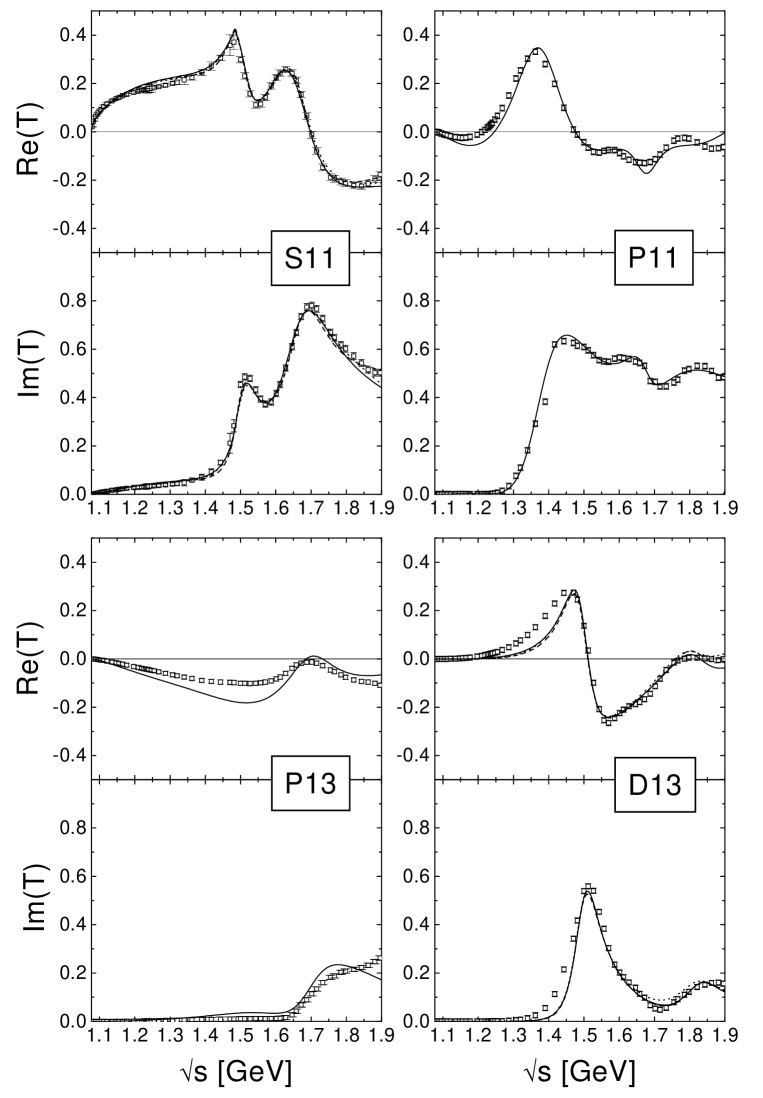
FIG. 1.: Fits to the $\pi N$ $I=\frac{1}{2}$-partial waves from KA84 [2]. Fit KA84-pt ( ), KA84-pp (     ) and KA84-ee ($\cdot\cdot\cdot$). For Notation see Sec. V.

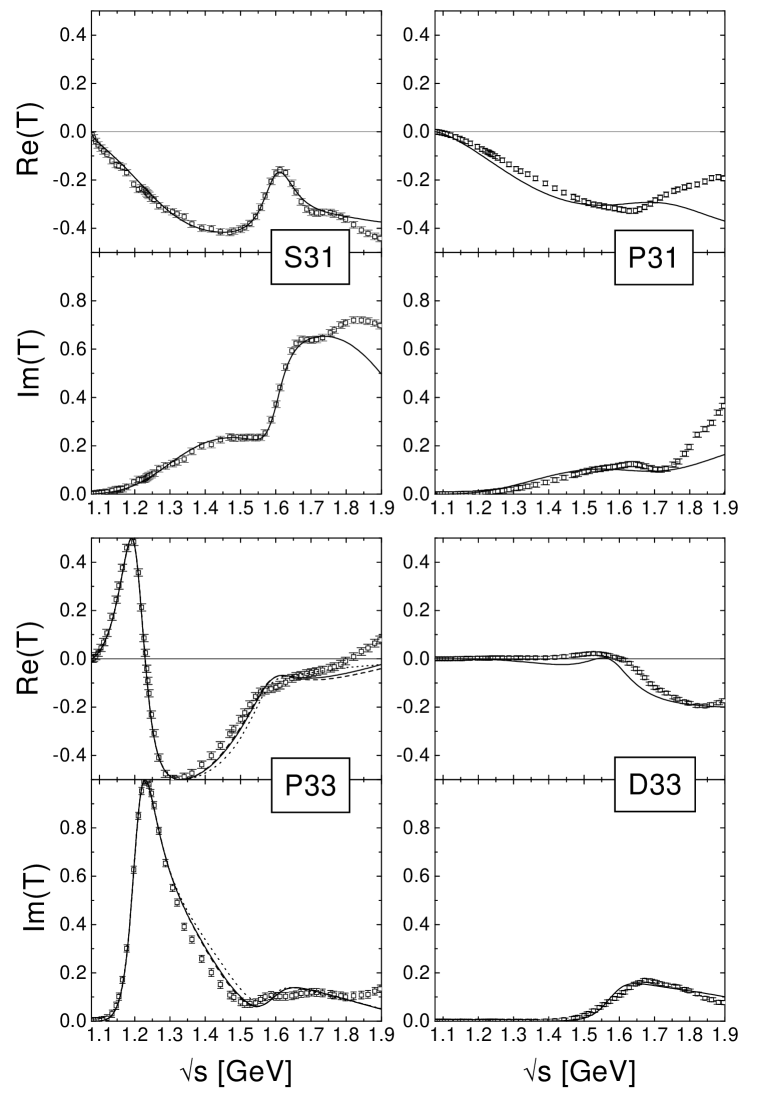
FIG. 2.: Results for the $I=\frac{3}{2}$-channels. Legend as in Fig. 1.

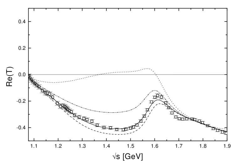
FIG. 3.: Influence of the $z_{\pi}$-parameter of the $P_{33}(1232)$ on the $S_{31}$-phase shift. KA84-pt ( ), $z_{\pi}=-0.5$ (     ), $z_{\pi}=0.0$ (   $\cdot\cdot$), no $P_{33}(1232)$ ($\cdot\cdot\cdot$).

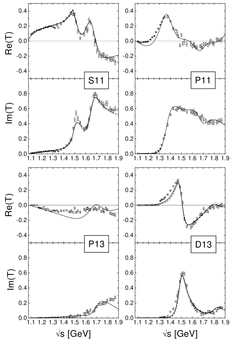
FIG. 4.: Fits to the $\pi N$ $I=\frac{1}{2}$-partial waves from SM95 [4]. Fit SM95-pt ( ), SM95-pp (     ) and SM95-ee ($\cdot\cdot\cdot$).

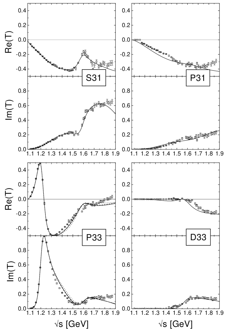
FIG. 5.: Results for the $I=\frac{3}{2}$-channels. Legend as in Fig. 4.

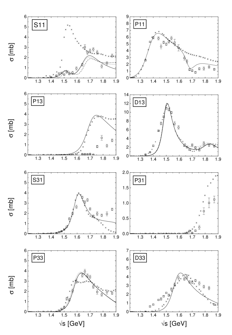
FIG. 6.: Comparison of the calculated $\pi N\to\pi\pi N$ cross sections for the fits using the KA84-PWA with the data from [3]. Legend as in Fig. 1. In addition the inelastic cross section as determined from the KA84-PWA is shown ($\times$).

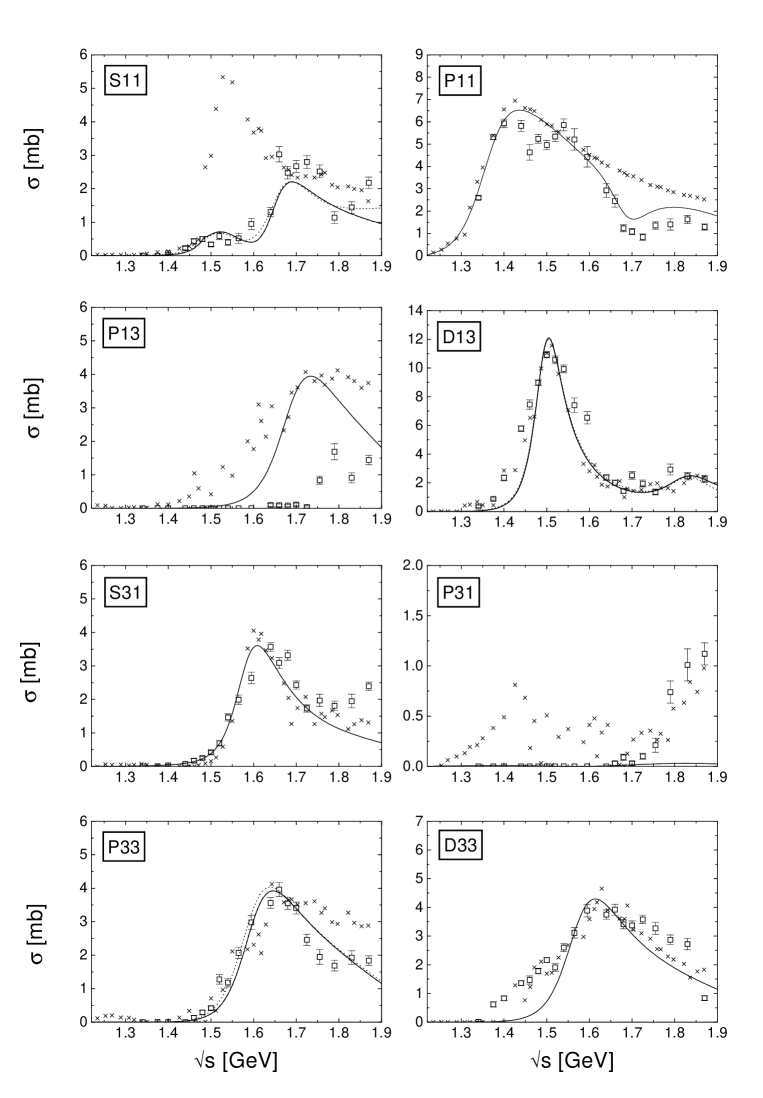
FIG. 7.: Comparison of the calculated $\pi N\to\pi\pi N$ cross sections for the fits using the SM95-PWA with the data from [3]. Legend as in Fig. 4. In addition the inelastic cross section as determined from the SM95-PWA is shown ($\times$).

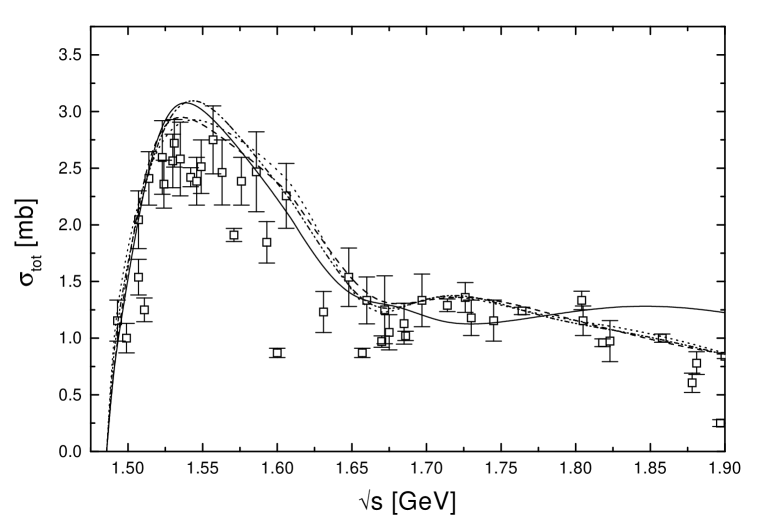
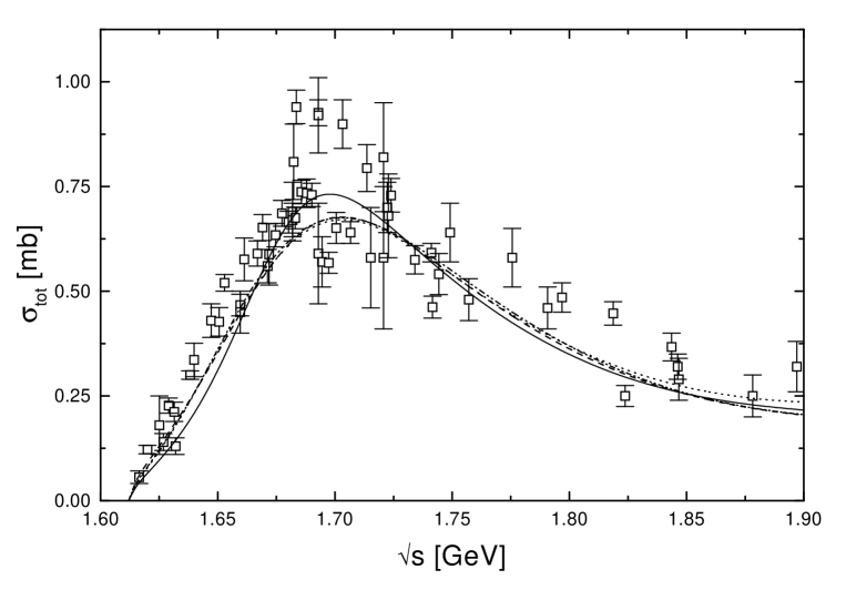
FIG. 8.: Results for the total $\pi^{-}p\to\eta n$ (upper plot) and $\pi^{-}p\to K^{0}\Lambda$ (lower) cross sections. Shown are the fits KA84-pt ( ), KA84-pp (     ), SM95-pt (   $\cdot\cdot$) and SM95-pp ($\cdot\cdot\cdot$). Data as in Figs. 9 and 11.

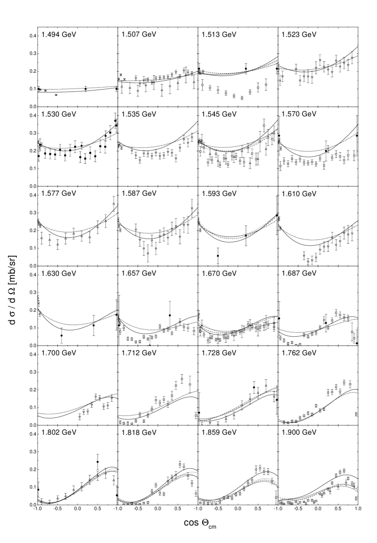
FIG. 9.: Comparison with data for the calculated differential $\pi^{-}p\to\eta n$ cross sections. Legend as in Fig. 8. The datapoints are taken from: [42] ($\bullet$), [43] ($\times$), [44] ($\bigtriangledown$), [45] ($\bigtriangleup$), [31] ($\Box$), [46] ( ).

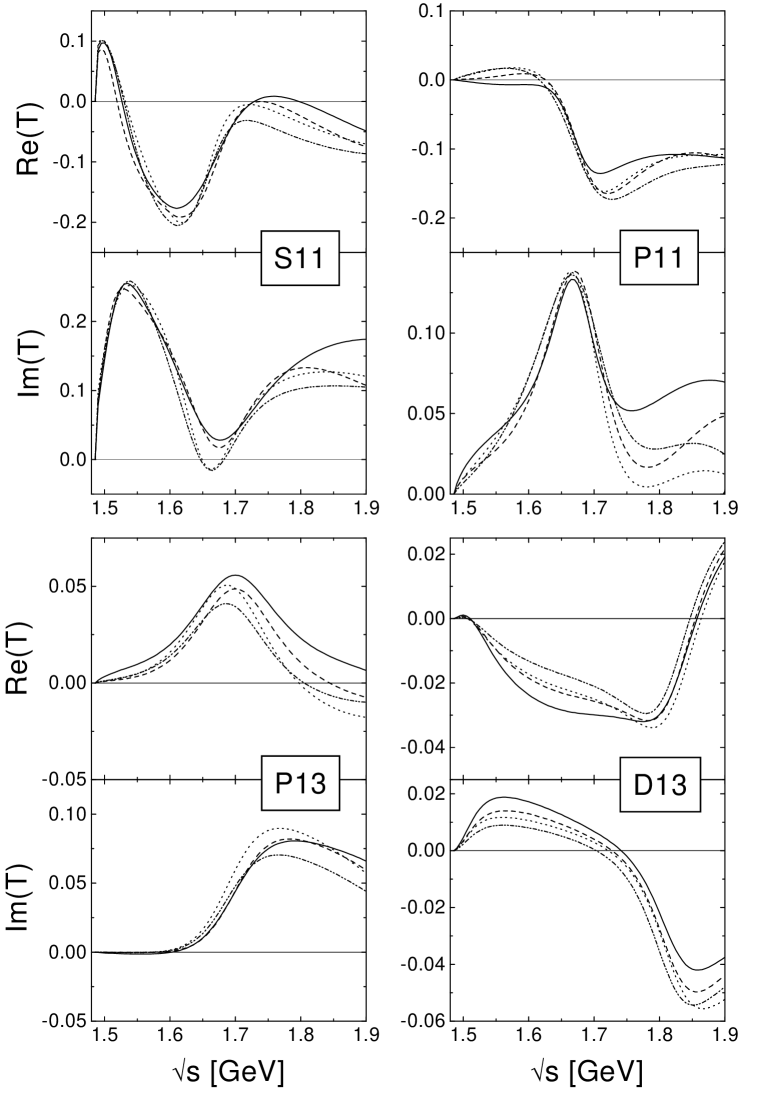
FIG. 10.: Calculated partial waves $T^{\frac{1}{2}}_{\pi\eta}$. Legend as in Fig. 8.

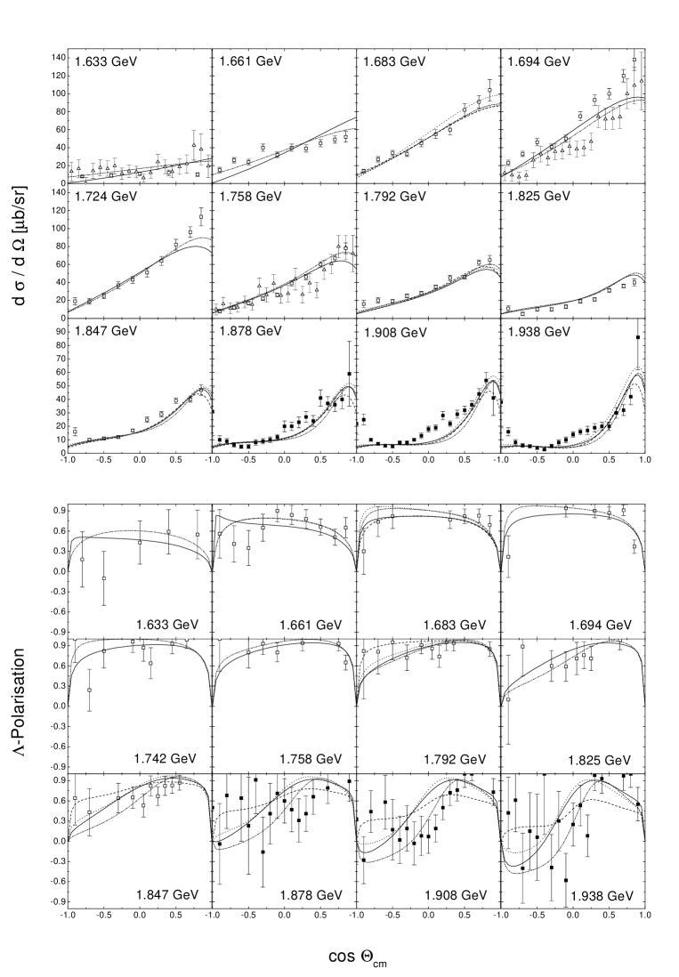
FIG. 11.: Comparison with data for the calculated differential $\pi^{-}p\to K^{0}\Lambda$ cross sections and $\Lambda$-polarizations. Legend as in Fig. 8. The datapoints are taken from: [47] ($\Box$), [48] ($\bigtriangleup$), [32] ( ).

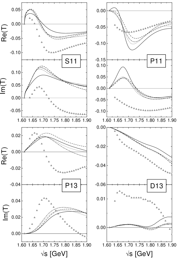
FIG. 12.: Calculated partial waves $T^{\frac{1}{2}}_{\pi K}$. Legend as in Fig. 8. In comparison also the results of the calculation of Sotona and Žofka [22] ($\bigtriangleup$) are shown.

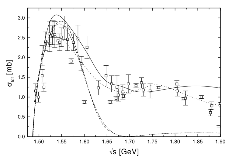
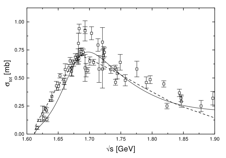
FIG. 13.: Comparison of the total $\pi^{-}p\to\eta n$ (upper plot) and $\pi^{-}p\to K^{0}\Lambda$ (lower) cross sections. Fit KA84-pt ( ), [12] (     ), [7] (   $\cdot\cdot$), [6] ($\cdot\cdot\cdot$). Data as in Figs. 9 and 11.

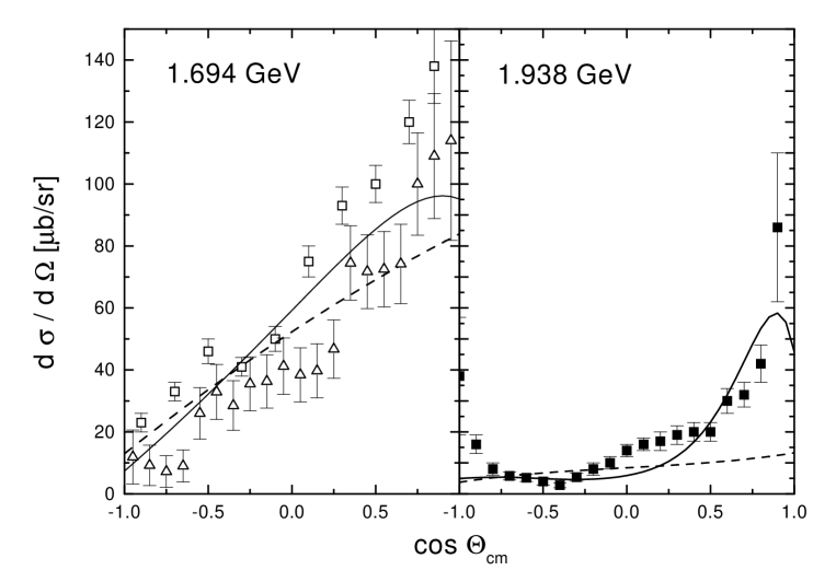
FIG. 14.: $K^{*}$-meson contribution to $\pi^{-}p\to K^{0}\Lambda$ for two different energies. Shown is the fit KA84-pt with ( ) and without (     ) the $K^{*}$.

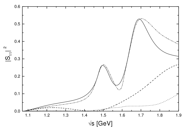
FIG. 15.: Comparison with the results from [34]. Plotted is the square of the absolute value of the $S_{11}$-phase shift. Fit KA84-pt ( ), background only (     ), full calculation (   $\cdot\cdot$) and background ($\cdot\cdot\cdot$) as given by [34].

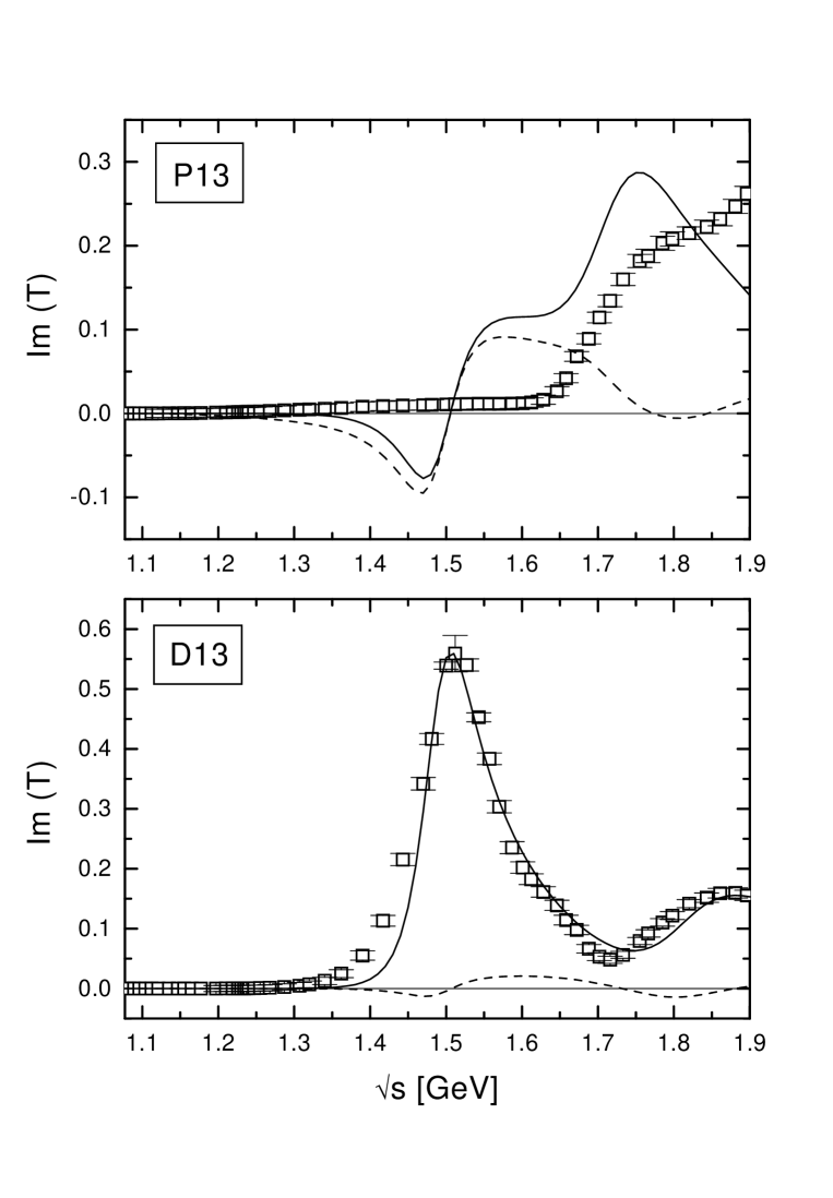
FIG. 16.: Results using the $T$-matrix approximation (38). Shown are the imaginary parts of the $P_{13}$- and $D_{13}$-partial waves for $\pi N$-scattering ( ) and the corresponding values $\Delta T^{\alpha}$ (     ). The data are from KA84 [2].

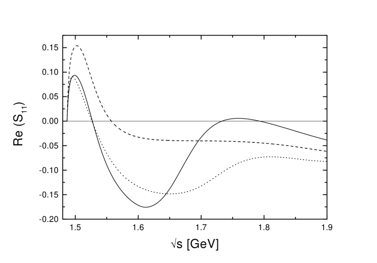
FIG. 17.: Influence of the $S_{11}(1650)$ on the $\pi N\to\eta N$ amplitudes. Shown is the real part of $S_{11}$ for the $K$-matrix calculation using KA84-pt with ( ) and without (     ) the $S_{11}(1650)$. For comparison we also show the $T$-matrix result ($\cdot\cdot\cdot$).

REFERENCES

- [1] R.E. Cutkosky, C.P. Forsyth, R.E. Hendrick and R.L. Kelly, Phys. Rev. D20, 2804, 2839 (1979); R.E. Cutkosky, C.P. Forsyth, J.B. Babcock, R.L. Kelly and R.E. Hendrick, Baryon 1980, Proc. 4th Int. Conf. on Baryon Resonances, ed. N. Isgur, p. 19
- [2] E. Pietarinen, Nucl. Phys. B107, 21 (1976); R. Koch, Nucl. Phys. A448, 707 (1986) and Z. Phys. C29, 597 (1985); G. Höhler, F. Kaiser, R. Koch and E. Pietarinen, Handbook of pion-nucleon scattering, Physics Data 12-1, Karlsruhe, 1979
- [3] D.M. Manley, R.A. Arndt, Y. Goradia and V.L. Teplitz, Phys. Rev. D30, 904 (1984) D.M. Manley and E.M. Saleski, Phys. Rev. D45, 4002 (1992)
- [4] SM95 and SP97 solutions of the VIRGINIA TECH PARTIAL-WAVE ANALYSIS, available via WWW from http://clsaid.phys.vt.eduCAPS. For further reference see, for example, R.A. Arndt, I.I. Strakovsky, R.L. Workman and M.M. Pavan, Phys. Rev. C52, 2120 (1995); R.A. Arndt, R.L. Workman, Z. Li and L.D. Roper, Phys. Rev. C42, 1853 (1990)
- [5] M. Benmerrouche, N.C. Mukhopadhyay and J.-F. Zhang, Phys. Rev. D51, 3237 (1995)
- [6] M. Batinić, I. Dadić, I. Šlaus, A. Švarc, B.M.K. Nefkens and T.-S.H. Lee, nucl-th@xxx.lanl.gov preprint #9703023; M. Batinić, I. Dadić, I. Šlaus, A. Švarc and B.M.K. Nefkens Phys. Rev. C51, 2310 (1995)
- [7] C. Sauermann, Ph.D. thesis, Darmstadt 1996; C. Deutsch-Sauermann, B. Friman and W. Noerenberg, Phys. Lett. B409, 51 (1997)
- [8] Particle Data Group, Phys. Rev. D54, 1 (1996)
- [9] S. Capstick and W. Roberts, Phys. Rev. D49, 4570 (1994)
- [10] L.Ya. Glozman and D.O. Riska, Phys. Lett. B366, 305 (1996)
- [11] R. Bijker, F. Iachello and A. Leviatan, Phys. Rev. D55, 2862 (1997)
- [12] N. Kaiser, T. Waas and W. Weise, Nucl. Phys. A612, 297 (1997)
- [13] M. Benmerrouche, R.M. Davidson and N.C. Mukhopadhyay, Phys. Rev. C39, 2339 (1989)
- [14] O. Scholten, A. Yu. Korchin, V. Pascalutsa and D. Van Neck, Phys. Lett. B384, 13 (1996)
- [15] T. Feuster and U. Mosel, Nucl. Phys. A612, 375 (1997)
- [16] G. Höhler, newsletter 9, 1 (1993)
- [17] B.C. Pearce and B.K. Jennings, Nucl. Phys. A528, 655 (1991)
- [18] T. Ericson and W. Weise, Pions and Nuclei, Calderon Press, Oxford, 1988
- [19] M. Gell-Mann and M. Levy, Nuovo Cim. 16, 53 (1960)
- [20] L.M. Nath and B.K. Bhattacharyya, Z. Phys. C5, 9 (1980)
- [21] P. van Nieuwenhuizen, Phys. Rep. 68, 228 (1981)
- [22] M. Sotona and J. Žofka, Prog. of Theo. Phys. 81, 160 (1989)
- [23] F. Klingl, N. Kaiser and W. Weise, hep-ph@xxx.lanl.gov preprint #9704398
- [24] L. Tiator, C. Bennhold and S.S. Kamalov, Nucl. Phys. A580, 455 (1994)
- [25] R.D. Peccei, Phys. Rev. 181, 1902 (1969)
- [26] S. Nozawa, B. Blankleider and T.-S.H. Lee, Nucl. Phys. A513, 459 (1990); S. Nozawa and T.-S.H. Lee, Nucl. Phys. A513, 511 (1990);
- [27] M.L. Goldberger and K.M. Watson, Collision Theory, Wiley, New York, 1964
- [28] J.D. Bjorken and S.D. Drell, Relativistic Quantummechanics, Bibliographisches Institut, Mannheim 1966
- [29] F. Hachenberg and H.J. Pirner, Ann. of Phys. 112, 401 (1978)
- [30] G. Höhler, Landolt-Börnstein Vol. 9, Springer, Berlin 1983
- [31] R.M. Brown et al., Nucl. Phys. B153, 89 (1979)
- [32] D.H. Saxon et al., Nucl. Phys. B162, 522 (1980)
- [33] C. Bennhold, T. Mart and D. Kusno, nucl-th@xxx.lanl.gov preprint #9703004
- [34] S.A. Dytman, T.P. Vrana and T.-S.H. Lee, nucl-th@xxx.lanl.gov preprint #9702033
- [35] G. Höhler and E. Pietarinen, Nucl. Phys. B95, 210 (1975)
- [36] B. Krusche et al., Phys. Rev. Lett. 74, 3736 (1995); Phys. Rev. Lett. 75, 3023 (1995); Phys. Lett. B358, 40 (1995)
- [37] M.G. Olsson, Nucl. Phys. B78, 55 (1974); M. G. Olsson and E. T. Osypowski, Nucl. Phys. B87, 399 (1975); Phys. Rev. D17, 174 (1978); Nucl. Phys. B101, 136 (1975)
- [38] R. Davidson, N.C. Mukhopadhyay and R. Wittman, Phys. Rev. D43, 71 (1991)
- [39] A.M. Green and S. Wycech, Phys. Rev. C55, 2167 (1997)
- [40] R.A. Adelseck and B. Saghai, Phys. Rev. C42, 108 (1990)
- [41] H. Thom, Phys. Rev. 151, 1322 (1966)
- [42] F. Bulos et al., Phys. Rev. 187, 1827 (1969)
- [43] N.C. Debenham et al., Phys. Rev. D12, 2545 (1975)
- [44] W. Deinet et al., Nucl. Phys. B11, 495 (1969)
- [45] B.W. Richards et al., Phys. Rev. D1, 10 (1970)
- [46] J. Feltesse et al., Nucl. Phys. B93, 242 (1975)
- [47] R.D. Baker et al., Nucl. Phys. B141, 29 (1978)
- [48] T.M. Knasel et al., Phys. Rev. D11, 1 (1975)