Relativistic Point-Coupling Models as
Effective Theories of Nuclei

Abstract

Recent studies have shown that concepts of effective field theory such as naturalness can be profitably applied to relativistic mean-field models of nuclei. Here the analysis by Friar, Madland, and Lynn of naturalness in a relativistic point-coupling model is extended. Fits to experimental nuclear data support naive dimensional analysis as a useful principle and imply a mean-field expansion analogous to that found for mean-field meson models.

I Introduction

Quantum Chromodynamics (QCD) is believed to be the underlying theory of hadrons and their interactions and therefore of nuclei as well. However, direct solutions of QCD for nuclei (e.g., lattice calculations) are not presently feasible. On the other hand, the modern perspective of effective field theory (EFT) [1, 2, 3, 4, 5, 6] provides a framework for constructing theories based on observed hadronic degrees of freedom that can faithfully reproduce low-energy QCD. An example of a successful EFT is chiral perturbation theory (ChPT)[1, 7, 8], which systematically describes low-energy hadronic processes in the vacuum.

The success of effective chiral lagrangians in the vacuum has motivated the application of EFT concepts to models of nuclear properties. A chiral effective lagrangian for nuclei was presented in Ref. [9], and has lead to new insights into the successes of quantum hadrodynamic (QHD) models[10, 11] of nuclei. In that work, a general model in which nucleons interact via mesonic degrees of freedom was constructed and applied to nuclei at the one-baryon-loop level (Hartree approximation).

The effective lagrangian and energy functional were organized according to Georgi’s naive dimensional analysis (NDA) [12, 13], which provides a controlled mean-field expansion in terms of powers and derivatives of the mean fields if the dimensionless coefficients identified in the NDA are of order one. The latter property is called “naturalness” in this context. Detailed fits to nuclear observables validated this expansion and truncation scheme [9]. This result is somewhat surprising since the NDA counting is based on absorbing short-distance physics into the coefficients of the effective lagrangian, but a mean-field functional fit to nuclear data must also absorb long-distance many-body effects.

A useful interpretation of the finite-density mean-field effective theory is in terms of density functional theory (DFT) [14, 15, 16, 17]. In a DFT formulation of the relativistic many-body problem, one works with an energy functional of scalar densities and vector four-currents. Minimization of the functional gives rise to variational equations that determine the ground-state densities. By introducing a complete set of Dirac wave functions, one can recast these variational equations as Dirac equations for occupied orbitals; the single-particle hamiltonian contains local scalar and vector potentials, not only in the Hartree approximation, but in the general case as well. The Hartree approximation only limits the form of the potentials. Thus the effects of many-body physics such as short-range correlations are incorporated (approximately) by a direct fit to nuclear observables.

In mean-field meson models, the scalar and vector meson fields play the role of auxiliary Kohn-Sham potentials. Alternatively, one can expand the local potentials directly in terms of nucleon densities. The corresponding lagrangian replaces meson exchange with point-coupling (contact) interactions. In Ref. [18], such a relativistic point-coupling lagrangian was introduced and applied to nuclei at the mean-field level. Subsequently, Friar et al. [19] examined this model for naturalness and concluded that the parameters were, in fact, mostly natural. Here, the analysis of point-coupling models in the context of EFT’s is reexamined and broadened in a manner consistent with the analysis of the chiral mean-field meson model of Ref. [9].

We find that the assumption of naturalness is justified and that the density expansion implied by NDA is applicable. In principle, the parameters found here could be related to those in the meson model of Ref. [9] by using the equations of motion in the lagrangian of [9] to systematically eliminate the meson fields. However, the point-coupling parameters are underdetermined by the fits, which limits the usefulness of the comparisons. New optimization procedures described below suggest that a different organization that exploits cancellations characteristic of relativistic models may be more productive.

II The Point-Coupling Lagrangian

At present we cannot derive an effective point-coupling lagrangian directly from QCD. In the same spirit as ChPT and the effective meson model of Ref. [9], a general point-coupling effective lagrangian is therefore constructed consistent with the underlying symmetries of QCD (e.g., Lorentz covariance, gauge invariance, and chiral symmetry). In this work, we construct a one-loop energy-functional from the lagrangian and determine the couplings by fits to nuclear observables. As noted above and discussed in Ref. [11], this approach approximates a density functional that, if sufficiently general, incorporates many-body effects beyond the Hartree approximation. We expect this approximation to be reasonable because of the large scalar and vector potentials (“Hartree dominance”) [9, 11].

This framework will only be useful if we can identify a valid expansion and truncation scheme. This requires an organization of terms in the effective lagrangian and a way to estimate the couplings. While precise relations between these couplings and the underlying QCD parameters are unknown, an estimate of the magnitude of the couplings can be obtained by applying Georgi’s naive dimensional analysis (NDA)[12, 9, 20].

The procedure is to extract from each term in the lagrangian the dependence on two primary physical scales of the effective theory, the pion decay constant, $f_{\pi}\approx 94\,$MeV and a larger mass scale, $\Lambda\sim 4\pi f_{\pi}/\sqrt{N_{f}}$ (where $N_{f}$ is the number of light flavors) [12, 13]. The scale $\Lambda$ is associated with the mass scale of physics beyond the Goldstone bosons (pions): the non-Goldstone boson masses or the nucleon mass. This mass scale ranges from the scalar mass $\approx 500\,$MeV to the baryon mass $\approx 1\,$GeV. When a specific value is needed in this work, $\Lambda$ will be taken to equal the $\rho$-meson mass ($770\,$MeV), roughly in the center of this range. To establish the canonical normalization of the strongly interacting fields, an inverse factor of $f_{\pi}$ is included for each field and an overall factor of $f_{\pi}^{2}\Lambda^{2}$ fixes the normalization of the lagrangian. The physics of NDA is discussed further in Refs. [9] and [11].

We construct the point-coupling effective lagrangian as an expansion in powers of the nucleon scalar, vector, isovector-vector, tensor, and isovector-tensor densities scaled according to NDA:

$${\widetilde{\rho}_{\scriptscriptstyle S}} \equiv {\rho_{\scriptscriptstyle S}\over f_{\pi}^{2}\Lambda}\equiv{\overline{N}N\over f_{\pi}^{2}\Lambda}\ ,$$ (1)

$$\widetilde{j}_{\scriptscriptstyle V}^{\mu} \equiv {j_{\scriptscriptstyle V}^{\mu}\over f_{\pi}^{2}\Lambda}\equiv{\overline{N}\gamma^{\mu}N\over f_{\pi}^{2}\Lambda}\ ,$$ (2)

$$\widetilde{j}_{{\mathchoice{{\hbox{\boldmath$\displaystyle\tau$}}}{{\hbox{\boldmath$\textstyle\tau$}}}{{\hbox{\boldmath$\scriptstyle\tau$}}}{{\hbox{\boldmath$\scriptscriptstyle\tau$}}}}}^{\mu} \equiv {j_{{\mathchoice{{\hbox{\boldmath$\displaystyle\tau$}}}{{\hbox{\boldmath$\textstyle\tau$}}}{{\hbox{\boldmath$\scriptstyle\tau$}}}{{\hbox{\boldmath$\scriptscriptstyle\tau$}}}}}^{\mu}\over f_{\pi}^{2}\Lambda}\equiv{\overline{N}\gamma^{\mu}{{\mathchoice{{\hbox{\boldmath$\displaystyle\tau$}}}{{\hbox{\boldmath$\textstyle\tau$}}}{{\hbox{\boldmath$\scriptstyle\tau$}}}{{\hbox{\boldmath$\scriptscriptstyle\tau$}}}}\over 2}N\over f_{\pi}^{2}\Lambda}\ ,$$ (3)

$$\widetilde{s}^{\mu\nu} \equiv {s^{\mu\nu}\over f_{\pi}^{2}\Lambda}\equiv{\overline{N}\sigma^{\mu\nu}N\over f_{\pi}^{2}\Lambda}\ ,$$ (4)

$$\widetilde{s}_{{\mathchoice{{\hbox{\boldmath$\displaystyle\tau$}}}{{\hbox{\boldmath$\textstyle\tau$}}}{{\hbox{\boldmath$\scriptstyle\tau$}}}{{\hbox{\boldmath$\scriptscriptstyle\tau$}}}}}^{\mu\nu} \equiv {s_{{\mathchoice{{\hbox{\boldmath$\displaystyle\tau$}}}{{\hbox{\boldmath$\textstyle\tau$}}}{{\hbox{\boldmath$\scriptstyle\tau$}}}{{\hbox{\boldmath$\scriptscriptstyle\tau$}}}}}^{\mu\nu}\over f_{\pi}^{2}\Lambda}\equiv{\overline{N}\sigma^{\mu\nu}{{\mathchoice{{\hbox{\boldmath$\displaystyle\tau$}}}{{\hbox{\boldmath$\textstyle\tau$}}}{{\hbox{\boldmath$\scriptstyle\tau$}}}{{\hbox{\boldmath$\scriptscriptstyle\tau$}}}}\over 2}N\over f_{\pi}^{2}\Lambda}\ ,$$ (5)

where $N$ is the nucleon field. The lagrangian is also organized according to an expansion in derivatives acting on these densities; NDA dictates that each derivative is scaled by $\Lambda$:

$${\widetilde{\partial}}^{\mu} \equiv {\partial^{\mu}\over\Lambda}\ .$$ (6)

Except for the kinetic term, derivatives acting on an individual nucleon field, rather than on a density, are eliminated by field redefinitions as in Ref. [9] in favor of terms of the form of Eqs. (1)–(5). This is because time derivatives on the nearly on-shell valence nucleons are of $O(M)$ and are therefore not suppressed according to (6). As discussed in Ref. [9], this procedure is only able to eliminate derivatives in the combination $\gamma^{\mu}\partial_{\mu}$ (and therefore $\partial^{\mu}\partial_{\mu}$). We can transform away mixed-derivative terms such as $(\overline{N}\partial_{\mu}N)(\overline{N}\partial^{\mu}N)$ in favor of tensor terms, which are then neglected (see below) [9].

Naive dimensional analysis provides an organizational principle that directly translates into numerical estimates at the mean-field level. For example, each additional power of $\rho_{s}$ is accompanied by a factor of $f_{\pi}^{2}\Lambda$. The ratios of scalar and vector densities to this factor at nuclear matter equilibrium density are between 1/4 and 1/7 [20], which serves as an expansion parameter. Similarly, one can anticipate good convergence for gradients of the densities, since the relevant scale for derivatives in finite nuclei should be roughly the nuclear surface thickness $\sigma$, and so the dimensionless expansion parameter is $1/\Lambda\sigma\leq 1/5$. This expansion is only useful, however, if the coefficients are not too large.

In effective lagrangians of QCD applied to scattering problems, fits to experimental data suggest that when NDA is applied the remaining dimensionless coefficients are of order unity. This is known as “naturalness”; it is an essential feature if NDA is to be useful as an organizational scheme. The premise of naturalness in point-coupling models is to be tested here for finite-density applications through fits to experimental nuclear data. Naive dimensional analysis applied to the point-coupling model of Nikolaus et al. [18, 19] and to the meson model of Ref. [9] already suggest that effective nuclear models are natural, which in turn implies a convergent mean-field expansion in density based on an organization prescribed by NDA [9]. This is a nontrivial result, because the naturalness assumption implies that all the short-distance physics (with scale $1/\Lambda$) is incorporated into the coefficients of the effective lagrangian, while long-distance finite-density effects should be calculated explicitly in a systematic application of the effective lagrangian. At the mean-field level, however, we also approximately absorb long-distance many-body effects from ladder and ring diagrams [11].

The effective lagrangian should in principle contain every possible term (allowed by symmetries) to a given order under this organization. However, certain classes of terms will be poorly determined by fits to bulk nuclear observables. Here meson-exchange phenomenology and experience with relativistic mean-field meson models are useful guides. Thus, we follow the physics motivation of Ref. [9] to determine which terms will be essential and which can be omitted. In particular, each term we include corresponds to one in the meson-nucleon lagrangian, as identified through a simple leading-order analysis. For example, at leading order, the scalar field, $\phi$, in the meson model of Ref. [9] is proportional to the scalar density, ${\widetilde{\rho}_{\scriptscriptstyle S}}$; terms second order in the scalar density here (including those containing derivatives) are therefore related to the mass and kinetic terms of the scalar meson field as well as its Yukawa coupling to the nucleon in the meson model. The term cubic in the scalar density in the point-coupling model has a correspondence with the term cubic in the scalar field, and so on. The absence of a tensor boson in the mesonic model corresponds to the absence of terms of the form $[\overline{N}\sigma^{\mu\nu}N]^{2}$ and $[{\widetilde{\partial}}_{\alpha}\overline{N}\sigma^{\mu\nu}N]^{2}$ in our point-coupling lagrangian. Tensor meson masses are large and tensor mean-field densities are small, so even if the coefficients are natural, we expect that such terms would have a small effect. An analysis of terms not included here is postponed to a future investigation.

The resulting point-coupling lagrangian is divided into four parts:

$${\cal L} = {\cal L}_{\rm NN}+{\cal L}_{\pi}+{\cal L}_{\rm EM}+{\cal L}_{\rm VMD}\ .$$ (7)

The pure nucleon contact interactions are contained in ${\cal L}_{\rm NN}$, and take the form

$${\cal L}_{\rm NN} = \overline{N}[i\partial^{\mu}\gamma_{\mu}-M]N$$ (13)

$$-f_{\pi}^{2}\Lambda^{2}\biggl{\{}\ {\widetilde{\rho}_{\scriptscriptstyle S}}^{2}\Bigl{[}\widetilde{\kappa}_{2}+\widetilde{\kappa}_{3}{\widetilde{\rho}_{\scriptscriptstyle S}}+\widetilde{\kappa}_{4}{\widetilde{\rho}_{\scriptscriptstyle S}}^{2}\Bigr{]}$$

$$\qquad\qquad\hbox{}+(\widetilde{j}_{\scriptscriptstyle V}^{\mu})^{2}\Bigl{[}\widetilde{\zeta}_{2}+\widetilde{\eta}_{1}{\widetilde{\rho}_{\scriptscriptstyle S}}+\widetilde{\eta}_{2}{\widetilde{\rho}_{\scriptscriptstyle S}}^{2}+\widetilde{\zeta}_{4}(\widetilde{j}_{\scriptscriptstyle V}^{\nu})^{2}\Bigr{]}$$

$$\qquad\qquad\hbox{}+[{\widetilde{\partial}}^{\mu}{\widetilde{\rho}_{\scriptscriptstyle S}}]^{2}\Bigl{[}\widetilde{\kappa}_{d}+\widetilde{\alpha}_{1}{\widetilde{\rho}_{\scriptscriptstyle S}}\Bigr{]}+[{\widetilde{\partial}}^{\mu}\widetilde{j}_{\scriptscriptstyle V}^{\nu}]^{2}\Bigl{[}\widetilde{\zeta}_{d}+\widetilde{\alpha}_{2}{\widetilde{\rho}_{\scriptscriptstyle S}}\Bigr{]}$$

$$\qquad\qquad\hbox{}+[\widetilde{j}_{{\mathchoice{{\hbox{\boldmath$\displaystyle\tau$}}}{{\hbox{\boldmath$\textstyle\tau$}}}{{\hbox{\boldmath$\scriptstyle\tau$}}}{{\hbox{\boldmath$\scriptscriptstyle\tau$}}}}}^{\mu}]^{2}\Bigl{[}\widetilde{\xi}_{2}+\widetilde{\eta}_{\rho}{\widetilde{\rho}_{\scriptscriptstyle S}}\Bigr{]}+{\widetilde{\xi}}_{d}[{\widetilde{\partial}}^{\mu}\widetilde{j}_{{\mathchoice{{\hbox{\boldmath$\displaystyle\tau$}}}{{\hbox{\boldmath$\textstyle\tau$}}}{{\hbox{\boldmath$\scriptstyle\tau$}}}{{\hbox{\boldmath$\scriptscriptstyle\tau$}}}}}^{\nu}]^{2}$$

$$\qquad\qquad\hbox{}+\widetilde{f}_{\rho}{\widetilde{\partial}}^{\mu}\widetilde{j}_{{\mathchoice{{\hbox{\boldmath$\displaystyle\tau$}}}{{\hbox{\boldmath$\textstyle\tau$}}}{{\hbox{\boldmath$\scriptstyle\tau$}}}{{\hbox{\boldmath$\scriptscriptstyle\tau$}}}}}^{\nu}\cdot{\widetilde{s}_{{\mathchoice{{\hbox{\boldmath$\displaystyle\tau$}}}{{\hbox{\boldmath$\textstyle\tau$}}}{{\hbox{\boldmath$\scriptstyle\tau$}}}{{\hbox{\boldmath$\scriptscriptstyle\tau$}}}}}}{}_{\mu\nu}+\widetilde{f}_{v}{\widetilde{\partial}}^{\mu}\widetilde{j}_{\scriptscriptstyle V}^{\nu}\widetilde{s}_{\mu\nu}\biggr{\}}\ .$$

The terms are organized to manifest the expansion and truncation of ${\cal L}$ in powers and derivatives of the densities. The point-coupling parameters have a “tilde” over them to distinguish them from the corresponding parameters of the hadron lagrangian in Ref. [9]. We follow Ref. [18] by not including counting factors in applying NDA, although they were included in Ref. [9]. This prescription will be tested empirically by our fits.

Compared to the point-coupling lagrangian of Nikolaus et al. [18], our lagrangian includes additional terms with coefficients $\widetilde{\eta}_{1}$, $\widetilde{\eta}_{2}$, $\widetilde{\alpha}_{1}$, $\widetilde{\alpha}_{2}$, $\widetilde{f}_{\rho}$, and $\widetilde{f}_{v}$. We also exclude contributions that would correspond to an isovector, scalar channel in the meson lagrangian. This meson was not included in Ref. [9] based on meson-exchange phenomenology, and we note that the corresponding point-coupling coefficient in [18] was found to be unnaturally small. Finally, we also postpone consideration of terms with an explicit dependence on the four-velocity $u^{\mu}$ of the nuclear medium (such as $u_{\mu}\widetilde{j}_{\scriptscriptstyle V}^{\mu}$), which might arise in an effective mean-field energy functional.

The electromagnetic kinetic and interaction terms are contained in ${\cal L}_{\rm EM}$ and ${\cal L}_{{\rm VMD}}$. Electromagnetic observables are calculated as an expansion in the electric charge $e$, as well as a derivative expansion. Here we work to first order in $e$; thus, only couplings to the nucleon that are linear in the photon field are considered. The lowest order terms in a derivative expansion are contained in ${\cal L}_{\rm EM}$ and take the same form as the photon-nucleon coupling terms in the meson model of Ref. [9]:

$${\cal L}_{\rm EM} = -{e\over 2}\overline{N}A^{\mu}\gamma_{\mu}(1+\tau_{3})N-{e\over 4M}F_{\mu\nu}\overline{N}\lambda\sigma^{\mu\nu}N$$ (15)

$$-{e\over 2M^{2}}\partial_{\nu}F^{\mu\nu}\overline{N}(\{\widetilde{\beta}_{s}+\widetilde{\beta}_{v}\tau_{3}\}\gamma_{\mu})N-{1\over 4}F^{\mu\nu}F_{\mu\nu}\ .$$

The anomalous magnetic moment, $\lambda$, is given by

$$\lambda={1\over 2}\lambda_{p}(1+\tau_{3})+{1\over 2}\lambda_{n}(1-\tau_{3})\ ,$$ (16)

where $\lambda_{p}$ and $\lambda_{n}$ are the anomalous moments for the proton and neutron.

In a mesonic model, an adequate description of the low-momentum electromagnetic form factors of a single nucleon is achieved through a combination of vector-meson dominance (VMD) [22, 23] and direct couplings of the photon to nucleons [9, 23]. Since heavy-meson degrees of freedom are eliminated here in favor of contact interactions, these effects must be expressed in the point-coupling model through direct higher-derivative couplings of the photon to the nucleon, contained in ${\cal L}_{\rm VMD}$. In practice we only include the next correction to the charge form factors:

$${\cal L}_{\rm VMD} = -{e\over M^{4}}\partial^{2}\partial_{\nu}F^{\mu\nu}\overline{N}(\{\widetilde{\delta}_{s}+\widetilde{\delta}_{v}\tau_{3}\}\gamma_{\mu})N\ .$$ (17)

The coefficients of ${\cal L}_{\rm EM}$ and ${\cal L}_{\rm VMD}$ are fixed by experimental electromagnetic data for protons and neutrons in the vacuum and are not varied independently when fitting to nuclear data. This is detailed below. The end result is that the composite electromagnetic structure of the nucleons is incorporated as a derivative expansion, which is appropriate for low-momentum physics. In the point-coupling model the expansion is constructed explicitly (at tree level) to a given order in momentum. In a meson model, vector meson dominance incorporates contributions to the form factor to all orders in the momentum.

The pion kinetic and interaction terms are contained in ${\cal L}_{\pi}$. The procedure for constructing this part of the lagrangian is similar to that presented for the meson model[9]. Since the pion field vanishes in the mean-field approximation, the details of its construction are not presented here, nor is an explicit form for these terms given. The pion will first enter when considering two-loop contributions to the energy.

Beyond a leading-order transformation from a meson lagrangian to a point-coupling lagrangian, the full expressions for the mean meson fields involve infinite series in powers of the various bilinears of the nucleon field. A precise transformation from the meson effective lagrangian at the mean-field level would therefore lead to the presence of higher-order terms in a point-coupling model that are treated here as negligible. In practice, because of delicate cancellations, a simple truncation of these terms leads to a poor fit with experimental data, but if the parameters are allowed to readjust slightly the new fit to the data is quite good.

This is not unlike the truncation of higher-order terms within the mean-field meson model: the inclusion of fifth-order terms (see Eq. (54) of Ref. [9]) into the lagrangian improves a fit to the data only marginally, but if the fifth-order terms are then simply truncated from the lagrangian, their effects must be absorbed into an adjustment of the lower-order coefficients if a good fit is to remain intact. Thus, the correspondence between the point-coupling model used here and the mean-field meson model of Ref. [9] is not exact due to truncations. Relations of the leading-order point-coupling coefficients here to the corresponding mean-field meson model coefficients that would result from a full transformation are listed below in Tables II, III, IV, and V.

In the meson model of Furnstahl et al.[9], the vector and $\rho$-meson masses are fixed at their vacuum values of $782\,$MeV and $770\,$MeV, respectively. The correspondences of these masses to the point-coupling parameters are given by

$$m_{v}^{2}=\widetilde{\zeta}_{2}/\widetilde{\zeta}_{d}\ ,\qquad m_{\rho}^{2} = \widetilde{\xi}_{2}/\widetilde{\xi}_{d}\ .$$ (18)

The vector meson and $\rho$-meson masses can therefore be “held fixed” within the point-coupling model by varying only $\widetilde{\zeta}_{2}$ and $\widetilde{\xi}_{2}$ and determining $\widetilde{\zeta}_{d}$ and ${\widetilde{\xi}}_{d}$ through these relations. These relations were not imposed in the point-coupling model studied by Hoch et al.[18]. Here we perform fits to experimental data both with these combinations fixed and allowing the four parameters to vary independently.

III Single-Nucleon Properties

The values of the photon coupling parameters $\lambda_{n}$, $\lambda_{p}$, $\widetilde{\beta}_{s}$, $\widetilde{\beta}_{v}$ and $\widetilde{\delta}_{\rm S}+\widetilde{\delta}_{\rm V}$ are all determined from single-nucleon electromagnetic form factors in the vacuum, calculated at tree level. The anomalous magnetic moments of the nucleon are fixed at $\lambda_{p}=1.793$ and $\lambda_{n}=-1.913$[9]. The other three parameters are related to the isoscalar and isovector charge form factors, which are given here for spacelike momenta $Q^{2}\equiv-q^{2}$ by

$$F_{1}^{s}(Q^{2})={1\over 2}-{\widetilde{\beta}_{s}\over 2M^{2}}Q^{2}-{\widetilde{\delta}_{s}\over M^{4}}Q^{4}+\cdots\ ;$$ (19)

$$F_{1}^{v}(Q^{2})={1\over 2}-{\widetilde{\beta}_{v}\over 2M^{2}}Q^{2}-{\widetilde{\delta}_{v}\over M^{4}}Q^{4}+\cdots\ .$$ (20)

The coefficients of the second-order terms are proportional to the corresponding mean-square charge radii, and their values are fixed from the experimental values [23]:

$$\widetilde{\beta}_{s} = M^{2}\langle r^{2}\rangle_{s1}/6\approx M^{2}(0.79\,{\rm fm})^{2}/6=2.36\ ,$$ (21)

$$\widetilde{\beta}_{v} = M^{2}\langle r^{2}\rangle_{v1}/6\approx M^{2}(0.79\,{\rm fm})^{2}/6=2.36\ .$$ (22)

These coefficients combine the direct coupling and VMD contributions that together determine the charge radii in the model of Ref. [9]. Unlike that model, there is no density dependence here from the effective masses of the vector mesons in medium. Since the difference between the point proton density and the full charge density is not very important in determining the self-consistent wavefunctions and energy levels, the point-coupling electromagnetic contributions produce similar results to the conventional convolution procedure [10], in which empirical single-nucleon form factors are folded with point nucleon densities after self-consistency is reached.

Nuclear structure observables do not depend strongly on the values of the fourth-order coefficients $\widetilde{\delta}_{s}$ and $\widetilde{\delta}_{v}$. Based on the criteria used here, the quality of fits are not affected by the inclusion of these parameters and their associated terms. They do play a key role in the (momentum-space) charge form-factor of each nucleus for higher values of $Q^{2}$, however. The d.m.s. charge radius, which depends on the position of the first zero of the charge form-factor $Q_{0}^{(1)}$[9]:

$$R_{\rm dms}\equiv 4.493/Q_{0}^{(1)}\ ,$$ (23)

is used as one criterion for optimization, and the parameter sets with good values of $\chi^{2}$ do reproduce the experimental result for the value of $Q_{0}^{(1)}$. However, if the fourth-order corrections are omitted, for oxygen there is a significant deviation from experiment beyond this value of momentum. In particular, the second maximum falls short of the predicted value (see Fig. 1). This is in contrast to the meson model, where vector-meson dominance yields the necessary momentum dependence to produce accurate results for the second maximum without including it as one of the criteria for optimization.

Fourth-order corrections in momentum are therefore included in the model through the parameters $\widetilde{\delta}_{s}$ and $\widetilde{\delta}_{v}$. A determination of the values of these parameters through vacuum properties is sufficient to reproduce the second maximum (see Fig. 1). In fact, due to the small magnitude of the neutron charge density in comparison to the proton, only the isospin $+1/2$ components of the additional terms are needed and $\widetilde{\delta}_{s}$ and $\widetilde{\delta}_{v}$ are therefore set equal.

FIG. 1.: Charge form factor of ¹⁶O. The solid line is taken from Ref. [24]. Form factors are shown for set FZ3 of the point-coupling model with and without fourth-order momentum corrections. Also, set G1 from the meson model [9] is shown.

We use a dipole fit to the proton form factor to determine the value of $\widetilde{\delta}_{s}=\widetilde{\delta}_{v}$. (Any alternative parameterization of the form factor could be used instead; our results are not sensitive to the details because it is a low-momentum expansion.) The proton form factor, $G_{E}^{p}(Q^{2})$ is known to be fitted well by a dipole form[25]:

$$G_{E}^{p}(Q^{2})=\left(1+\alpha{Q^{2}\over M^{2}}\right)^{-2}=1-2\alpha{Q^{2}\over M^{2}}+3\alpha^{2}{Q^{4}\over M^{4}}+\cdots\ .$$ (24)

This form factor is related to the isoscalar and isovector form factors by the relation

$$G_{E}^{p}(Q^{2})=F^{p}_{1}(Q^{2})-{Q^{2}\over 4M^{2}}F^{p}_{2}(Q^{2})\ ,$$ (25)

where

$$F_{i}^{p}(Q^{2})\equiv F_{i}^{s}(Q^{2})+F_{i}^{v}(Q^{2})\ .$$ (26)

Using Eqs. (19) and (20) and the fact that $\widetilde{\delta}_{s}=\widetilde{\delta}_{v}$, the proton form factor in Eq. (25) can be expanded as

$$G_{E}^{p}(Q^{2})=1-{2\widetilde{\beta}_{s}+2\widetilde{\beta}_{v}+\lambda_{p}\over 4M^{2}}Q^{2}-{2\widetilde{\delta}_{s}\over M^{4}}Q^{4}+\cdots\ .$$ (27)

Comparison with Eq.(24) yields

$$\alpha={\textstyle 2\widetilde{\beta}_{s}+2\widetilde{\beta}_{v}+\lambda_{p}\over\mathstrut\textstyle 8}=1.39\ ;$$ (28)

$$2\widetilde{\delta}_{s}=-3\alpha^{2}=-5.80\ .$$ (29)

In principle, higher-order momentum corrections to the anomalous form factors $F_{2}^{s,v}$, which are not considered here, would lead to an additional $Q^{4}$ dependence to the proton form-factor. Our sole interest is in determining the overall coefficient appearing at fourth-order in Eq. (27), however, and such a contribution could be re-absorbed into a redefinition of $\widetilde{\delta}_{s}$.

IV The Mean-Field Solutions

We work at one-baryon-loop order in this paper, which is equivalent to the Dirac-Hartree approximation [10]. This should be sufficient to test the consistency of naturalness through NDA and the truncation of the lagrangian. As discussed in Ref. [26], a Hartree calculation can be viewed as equivalent to a density-functional approach, in which higher-order many-body corrections are treated approximately. Such corrections have not yet been explored in a relativistic point-coupling model. In future work, the stability of the Hartree results will be tested in a two-loop calculation.

From the lagrangian, one can derive the Dirac equation and the energy functional for nuclei conventionally, keeping in mind that there are time derivatives acting on $\psi^{\dagger}$ as well as $\psi$. (See Ref. [18] for details.) Because of its large mass, loop integrals with the nucleon include dynamics from distance scales that are much shorter than the scale set by the valence-nucleon momenta, which are limited by the Fermi momentum $k_{\rm F}$. These short-range effects are included implicitly in the coefficients of the lagrangian and energy functional. Formally, one can include counterterms to remove these loop effects to all orders, which is always possible, since all such terms are already contained in the effective lagrangian.

The single-particle Dirac hamiltonian for spherically symmetric nuclei takes a form similar to that of Ref. [9]:

$$h({\bf x}) = -i\mathchoice{{\hbox{\boldmath$\displaystyle\alpha\cdot$}}}{{\hbox{\boldmath$\textstyle\alpha\cdot$}}}{{\hbox{\boldmath$\scriptstyle\alpha\cdot$}}}{{\hbox{\boldmath$\scriptscriptstyle\alpha\cdot$}}}{\mathchoice{{\hbox{\boldmath$\displaystyle\nabla$}}}{{\hbox{\boldmath$\textstyle\nabla$}}}{{\hbox{\boldmath$\scriptstyle\nabla$}}}{{\hbox{\boldmath$\scriptscriptstyle\nabla$}}}}+W(r)+{1\over 2}\tau_{3}R(r)+\beta(M-\Phi(r))+i\beta\mathchoice{{\hbox{\boldmath$\displaystyle\alpha\cdot T$}}}{{\hbox{\boldmath$\textstyle\alpha\cdot T$}}}{{\hbox{\boldmath$\scriptstyle\alpha\cdot T$}}}{{\hbox{\boldmath$\scriptscriptstyle\alpha\cdot T$}}}(r)+{i\over 2}\beta\mathchoice{{\hbox{\boldmath$\displaystyle\alpha\cdot T$}}}{{\hbox{\boldmath$\textstyle\alpha\cdot T$}}}{{\hbox{\boldmath$\scriptstyle\alpha\cdot T$}}}{{\hbox{\boldmath$\scriptscriptstyle\alpha\cdot T$}}}_{3}(r)\tau_{3}$$ (32)

$$+{1\over 2}(1+\tau_{3})A(r)+{1\over 2M^{2}}(\beta_{s}+\beta_{v}\tau_{3}){\mathchoice{{\hbox{\boldmath$\displaystyle\nabla$}}}{{\hbox{\boldmath$\textstyle\nabla$}}}{{\hbox{\boldmath$\scriptstyle\nabla$}}}{{\hbox{\boldmath$\scriptscriptstyle\nabla$}}}}^{2}A(r)-{1\over M^{4}}(\delta_{s}+\delta_{v}\tau_{3})({\mathchoice{{\hbox{\boldmath$\displaystyle\nabla$}}}{{\hbox{\boldmath$\textstyle\nabla$}}}{{\hbox{\boldmath$\scriptstyle\nabla$}}}{{\hbox{\boldmath$\scriptscriptstyle\nabla$}}}}^{2})^{2}A(r)$$

$$-{i\over 4M}[\lambda_{p}(1+\tau_{3})+\lambda_{n}(1-\tau_{3})]\beta\mathchoice{{\hbox{\boldmath$\displaystyle\alpha\cdot$}}}{{\hbox{\boldmath$\textstyle\alpha\cdot$}}}{{\hbox{\boldmath$\scriptstyle\alpha\cdot$}}}{{\hbox{\boldmath$\scriptscriptstyle\alpha\cdot$}}}{\mathchoice{{\hbox{\boldmath$\displaystyle\nabla$}}}{{\hbox{\boldmath$\textstyle\nabla$}}}{{\hbox{\boldmath$\scriptstyle\nabla$}}}{{\hbox{\boldmath$\scriptscriptstyle\nabla$}}}}A(r)\ ,$$

where the potentials $\Phi$, $W$, $R$, $A$, $\textstyle T$, and $\mathchoice{{\hbox{\boldmath$\displaystyle T$}}}{{\hbox{\boldmath$\textstyle T$}}}{{\hbox{\boldmath$\scriptstyle T$}}}{{\hbox{\boldmath$\scriptscriptstyle T$}}}_{3}$ are defined by

$$\Phi \equiv -\Lambda\{2\widetilde{\kappa}_{2}{\widetilde{\rho}_{\scriptscriptstyle S}}+2\widetilde{\kappa}_{d}{\widetilde{\mathchoice{{\hbox{\boldmath$\displaystyle\nabla$}}}{{\hbox{\boldmath$\textstyle\nabla$}}}{{\hbox{\boldmath$\scriptstyle\nabla$}}}{{\hbox{\boldmath$\scriptscriptstyle\nabla$}}}}}^{2}{\widetilde{\rho}_{\scriptscriptstyle S}}+3\widetilde{\kappa}_{3}{\widetilde{\rho}_{\scriptscriptstyle S}}^{2}+4\widetilde{\kappa}_{4}{\widetilde{\rho}_{\scriptscriptstyle S}}^{3}+\widetilde{\eta}_{1}(\widetilde{j}_{\scriptscriptstyle V}^{0})^{2}+2\widetilde{\eta}_{2}(\widetilde{j}_{\scriptscriptstyle V}^{0})^{2}{\widetilde{\rho}_{\scriptscriptstyle S}}+\widetilde{\eta}_{\rho}(\widetilde{j}_{{\mathchoice{{\hbox{\boldmath$\displaystyle\tau$}}}{{\hbox{\boldmath$\textstyle\tau$}}}{{\hbox{\boldmath$\scriptstyle\tau$}}}{{\hbox{\boldmath$\scriptscriptstyle\tau$}}}}}^{0})^{2}$$ (34)

$$\hbox{}+\widetilde{\alpha}_{1}({\widetilde{\mathchoice{{\hbox{\boldmath$\displaystyle\nabla$}}}{{\hbox{\boldmath$\textstyle\nabla$}}}{{\hbox{\boldmath$\scriptstyle\nabla$}}}{{\hbox{\boldmath$\scriptscriptstyle\nabla$}}}}}{\widetilde{\rho}_{\scriptscriptstyle S}})^{2}+2\widetilde{\alpha}_{1}{\widetilde{\rho}_{\scriptscriptstyle S}}{\widetilde{\mathchoice{{\hbox{\boldmath$\displaystyle\nabla$}}}{{\hbox{\boldmath$\textstyle\nabla$}}}{{\hbox{\boldmath$\scriptstyle\nabla$}}}{{\hbox{\boldmath$\scriptscriptstyle\nabla$}}}}}^{2}{\widetilde{\rho}_{\scriptscriptstyle S}}-\widetilde{\alpha}_{2}({\widetilde{\mathchoice{{\hbox{\boldmath$\displaystyle\nabla$}}}{{\hbox{\boldmath$\textstyle\nabla$}}}{{\hbox{\boldmath$\scriptstyle\nabla$}}}{{\hbox{\boldmath$\scriptscriptstyle\nabla$}}}}}\widetilde{j}_{\scriptscriptstyle V}^{0})^{2}\}\ ,$$

$$W \equiv \Lambda\{2\widetilde{\zeta}_{2}(\widetilde{j}_{\scriptscriptstyle V}^{0})+2\widetilde{\zeta}_{d}{\widetilde{\mathchoice{{\hbox{\boldmath$\displaystyle\nabla$}}}{{\hbox{\boldmath$\textstyle\nabla$}}}{{\hbox{\boldmath$\scriptstyle\nabla$}}}{{\hbox{\boldmath$\scriptscriptstyle\nabla$}}}}}^{2}(\widetilde{j}_{\scriptscriptstyle V}^{0})+4\widetilde{\zeta}_{4}(\widetilde{j}_{\scriptscriptstyle V}^{0})^{3}+2\widetilde{\eta}_{1}\widetilde{j}_{\scriptscriptstyle V}^{0}{\widetilde{\rho}_{\scriptscriptstyle S}}+2\widetilde{\eta}_{2}\widetilde{j}_{\scriptscriptstyle V}^{0}{\widetilde{\rho}_{\scriptscriptstyle S}}^{2}$$ (36)

$$\hbox{}+2\widetilde{\alpha}_{2}({\widetilde{\mathchoice{{\hbox{\boldmath$\displaystyle\nabla$}}}{{\hbox{\boldmath$\textstyle\nabla$}}}{{\hbox{\boldmath$\scriptstyle\nabla$}}}{{\hbox{\boldmath$\scriptscriptstyle\nabla$}}}}}{\widetilde{\rho}_{\scriptscriptstyle S}}\mathchoice{{\hbox{\boldmath$\displaystyle\cdot$}}}{{\hbox{\boldmath$\textstyle\cdot$}}}{{\hbox{\boldmath$\scriptstyle\cdot$}}}{{\hbox{\boldmath$\scriptscriptstyle\cdot$}}}{\widetilde{\mathchoice{{\hbox{\boldmath$\displaystyle\nabla$}}}{{\hbox{\boldmath$\textstyle\nabla$}}}{{\hbox{\boldmath$\scriptstyle\nabla$}}}{{\hbox{\boldmath$\scriptscriptstyle\nabla$}}}}}\widetilde{j}_{\scriptscriptstyle V}^{0}+{\widetilde{\rho}_{\scriptscriptstyle S}}{\widetilde{\mathchoice{{\hbox{\boldmath$\displaystyle\nabla$}}}{{\hbox{\boldmath$\textstyle\nabla$}}}{{\hbox{\boldmath$\scriptstyle\nabla$}}}{{\hbox{\boldmath$\scriptscriptstyle\nabla$}}}}}^{2}\widetilde{j}_{\scriptscriptstyle V}^{0})+\widetilde{f}_{v}{\widetilde{\mathchoice{{\hbox{\boldmath$\displaystyle\nabla$}}}{{\hbox{\boldmath$\textstyle\nabla$}}}{{\hbox{\boldmath$\scriptstyle\nabla$}}}{{\hbox{\boldmath$\scriptscriptstyle\nabla$}}}}}\mathchoice{{\hbox{\boldmath$\displaystyle\cdot\widetilde{s}$}}}{{\hbox{\boldmath$\textstyle\cdot\widetilde{s}$}}}{{\hbox{\boldmath$\scriptstyle\cdot\widetilde{s}$}}}{{\hbox{\boldmath$\scriptscriptstyle\cdot\widetilde{s}$}}}\}\ ,$$

$$R \equiv \Lambda\{2\widetilde{\xi}_{2}\widetilde{j}_{{\mathchoice{{\hbox{\boldmath$\displaystyle\tau$}}}{{\hbox{\boldmath$\textstyle\tau$}}}{{\hbox{\boldmath$\scriptstyle\tau$}}}{{\hbox{\boldmath$\scriptscriptstyle\tau$}}}}}^{0}+2\widetilde{\xi}_{d}{\widetilde{\mathchoice{{\hbox{\boldmath$\displaystyle\nabla$}}}{{\hbox{\boldmath$\textstyle\nabla$}}}{{\hbox{\boldmath$\scriptstyle\nabla$}}}{{\hbox{\boldmath$\scriptscriptstyle\nabla$}}}}}^{2}\widetilde{j}_{{\mathchoice{{\hbox{\boldmath$\displaystyle\tau$}}}{{\hbox{\boldmath$\textstyle\tau$}}}{{\hbox{\boldmath$\scriptstyle\tau$}}}{{\hbox{\boldmath$\scriptscriptstyle\tau$}}}}}^{0}+2\widetilde{\eta}_{\rho}{\widetilde{\rho}_{\scriptscriptstyle S}}\widetilde{j}_{{\mathchoice{{\hbox{\boldmath$\displaystyle\tau$}}}{{\hbox{\boldmath$\textstyle\tau$}}}{{\hbox{\boldmath$\scriptstyle\tau$}}}{{\hbox{\boldmath$\scriptscriptstyle\tau$}}}}}^{0}+\widetilde{f}_{\rho}{\widetilde{\mathchoice{{\hbox{\boldmath$\displaystyle\nabla$}}}{{\hbox{\boldmath$\textstyle\nabla$}}}{{\hbox{\boldmath$\scriptstyle\nabla$}}}{{\hbox{\boldmath$\scriptscriptstyle\nabla$}}}}}\mathchoice{{\hbox{\boldmath$\displaystyle\cdot\widetilde{s}_{{\mathchoice{{\hbox{\boldmath$\displaystyle\tau$}}}{{\hbox{\boldmath$\textstyle\tau$}}}{{\hbox{\boldmath$\scriptstyle\tau$}}}{{\hbox{\boldmath$\scriptscriptstyle\tau$}}}}}$}}}{{\hbox{\boldmath$\textstyle\cdot\widetilde{s}_{{\mathchoice{{\hbox{\boldmath$\displaystyle\tau$}}}{{\hbox{\boldmath$\textstyle\tau$}}}{{\hbox{\boldmath$\scriptstyle\tau$}}}{{\hbox{\boldmath$\scriptscriptstyle\tau$}}}}}$}}}{{\hbox{\boldmath$\scriptstyle\cdot\widetilde{s}_{{\mathchoice{{\hbox{\boldmath$\displaystyle\tau$}}}{{\hbox{\boldmath$\textstyle\tau$}}}{{\hbox{\boldmath$\scriptstyle\tau$}}}{{\hbox{\boldmath$\scriptscriptstyle\tau$}}}}}$}}}{{\hbox{\boldmath$\scriptscriptstyle\cdot\widetilde{s}_{{\mathchoice{{\hbox{\boldmath$\displaystyle\tau$}}}{{\hbox{\boldmath$\textstyle\tau$}}}{{\hbox{\boldmath$\scriptstyle\tau$}}}{{\hbox{\boldmath$\scriptscriptstyle\tau$}}}}}$}}}\}\ ,$$ (37)

$$A \equiv eA_{0}\ ;$$ (38)

$$T \equiv -\Lambda\widetilde{f}_{v}{\widetilde{\mathchoice{{\hbox{\boldmath$\displaystyle\nabla$}}}{{\hbox{\boldmath$\textstyle\nabla$}}}{{\hbox{\boldmath$\scriptstyle\nabla$}}}{{\hbox{\boldmath$\scriptscriptstyle\nabla$}}}}}\widetilde{j}_{\scriptscriptstyle V}^{0}\ ,$$ (39)

$$\mathchoice{{\hbox{\boldmath$\displaystyle T$}}}{{\hbox{\boldmath$\textstyle T$}}}{{\hbox{\boldmath$\scriptstyle T$}}}{{\hbox{\boldmath$\scriptscriptstyle T$}}}_{3} \equiv -\Lambda\widetilde{f}_{\rho}{\widetilde{\mathchoice{{\hbox{\boldmath$\displaystyle\nabla$}}}{{\hbox{\boldmath$\textstyle\nabla$}}}{{\hbox{\boldmath$\scriptstyle\nabla$}}}{{\hbox{\boldmath$\scriptscriptstyle\nabla$}}}}}\widetilde{j}_{{\mathchoice{{\hbox{\boldmath$\displaystyle\tau$}}}{{\hbox{\boldmath$\textstyle\tau$}}}{{\hbox{\boldmath$\scriptstyle\tau$}}}{{\hbox{\boldmath$\scriptscriptstyle\tau$}}}}}^{0}\ ,$$ (40)

$$\mathchoice{{\hbox{\boldmath$\displaystyle\widetilde{s}$}}}{{\hbox{\boldmath$\textstyle\widetilde{s}$}}}{{\hbox{\boldmath$\scriptstyle\widetilde{s}$}}}{{\hbox{\boldmath$\scriptscriptstyle\widetilde{s}$}}}_{i} \equiv \widetilde{s}_{0i}\ ,$$ (41)

$$\mathchoice{{\hbox{\boldmath$\displaystyle\widetilde{s}_{{\mathchoice{{\hbox{\boldmath$\displaystyle\tau$}}}{{\hbox{\boldmath$\textstyle\tau$}}}{{\hbox{\boldmath$\scriptstyle\tau$}}}{{\hbox{\boldmath$\scriptscriptstyle\tau$}}}}}$}}}{{\hbox{\boldmath$\textstyle\widetilde{s}_{{\mathchoice{{\hbox{\boldmath$\displaystyle\tau$}}}{{\hbox{\boldmath$\textstyle\tau$}}}{{\hbox{\boldmath$\scriptstyle\tau$}}}{{\hbox{\boldmath$\scriptscriptstyle\tau$}}}}}$}}}{{\hbox{\boldmath$\scriptstyle\widetilde{s}_{{\mathchoice{{\hbox{\boldmath$\displaystyle\tau$}}}{{\hbox{\boldmath$\textstyle\tau$}}}{{\hbox{\boldmath$\scriptstyle\tau$}}}{{\hbox{\boldmath$\scriptscriptstyle\tau$}}}}}$}}}{{\hbox{\boldmath$\scriptscriptstyle\widetilde{s}_{{\mathchoice{{\hbox{\boldmath$\displaystyle\tau$}}}{{\hbox{\boldmath$\textstyle\tau$}}}{{\hbox{\boldmath$\scriptstyle\tau$}}}{{\hbox{\boldmath$\scriptscriptstyle\tau$}}}}}$}}}_{i} \equiv \widetilde{s}_{{\mathchoice{{\hbox{\boldmath$\displaystyle\tau$}}}{{\hbox{\boldmath$\textstyle\tau$}}}{{\hbox{\boldmath$\scriptstyle\tau$}}}{{\hbox{\boldmath$\scriptscriptstyle\tau$}}}}}{}_{0i}\ .$$ (42)

The Dirac equation with eigenvalues $E_{\alpha}$ and eigenfunctions $N_{\alpha}({\bf x})$ is

$$hN_{\alpha}({\bf x})=E_{\alpha}N_{\alpha}({\bf x})\ ,\qquad\qquad\int\!d^{3}x\ N^{\dagger}_{\alpha}({\bf x})N_{\alpha}({\bf x})=1\ .$$ (43)

Following the conventions of Ref. [10] (also used in Ref. [9]), the eigenfunctions for spherically symmetric nuclei are written in terms of spin spherical harmonics, $\Phi_{\kappa m}$:

$$N_{\alpha} = N_{n\kappa mt}=\left(\matrix{{\textstyle i\over\textstyle r}G_{a}(r)\Phi_{\kappa m}\cr-{\textstyle 1\over\textstyle r}F_{a}(r)\Phi_{-\kappa m}}\right)\zeta_{t}\ ,$$ (44)

where $t=1/2$ for protons and $t=-1/2$ for neutrons. The equation for $N_{\alpha}$ then reduces to a set of coupled equations for $G_{a}$ and $F_{a}$:

$$\left({d\over dr}+{\kappa\over r}\right)G_{a}(r)-[E_{\alpha}-U_{1}(r)+U_{2}(r)]F_{a}(r)-U_{3}(r)G_{a}(r)=0\ ,$$ (45)

$$\left({d\over dr}-{\kappa\over r}\right)+[E_{\alpha}-U_{1}(r)-U_{2}(r)]G_{a}(r)+U_{3}(r)F_{a}(r)=0\ ,$$ (46)

where we have defined the single-particle potentials by

$$U_{1}(r) = W(r)+t_{a}R(r)+(t_{a}+1/2)A(r)+{1\over 2M^{2}}(\widetilde{\beta}_{s}+2t_{a}\widetilde{\beta}_{v}){\mathchoice{{\hbox{\boldmath$\displaystyle\nabla$}}}{{\hbox{\boldmath$\textstyle\nabla$}}}{{\hbox{\boldmath$\scriptstyle\nabla$}}}{{\hbox{\boldmath$\scriptscriptstyle\nabla$}}}}^{2}A(r)$$ (48)

$$\quad-{1\over M^{4}}(\widetilde{\delta}_{s}+2t_{a}\widetilde{\delta}_{v})({\mathchoice{{\hbox{\boldmath$\displaystyle\nabla$}}}{{\hbox{\boldmath$\textstyle\nabla$}}}{{\hbox{\boldmath$\scriptstyle\nabla$}}}{{\hbox{\boldmath$\scriptscriptstyle\nabla$}}}}^{2})^{2}A(r)\ ,$$

$$U_{2}(r) = M-\Phi(r)\ ,$$ (49)

$$U_{3}(r) = -\mathchoice{{\hbox{\boldmath$\displaystyle T$}}}{{\hbox{\boldmath$\textstyle T$}}}{{\hbox{\boldmath$\scriptstyle T$}}}{{\hbox{\boldmath$\scriptscriptstyle T$}}}(r)\cdot\hat{r}-t_{a}\mathchoice{{\hbox{\boldmath$\displaystyle T_{3}$}}}{{\hbox{\boldmath$\textstyle T_{3}$}}}{{\hbox{\boldmath$\scriptstyle T_{3}$}}}{{\hbox{\boldmath$\scriptscriptstyle T_{3}$}}}(r)\cdot\hat{r}+{1\over 2M}[(\lambda_{p}+\lambda_{n})/2+t_{a}(\lambda_{p}-\lambda_{n})]{dA\over dr}\ .$$ (50)

The mean-field densities can be expressed in terms of the radial wave functions $G$ and $F$ in the same manner as Refs. [9] and [10]:

$${\widetilde{\rho}_{\scriptscriptstyle S}}(r) = {1\over f_{\pi}^{2}\Lambda}\sum_{a}^{\rm occ}{2j_{a}+1\over 4\pi r^{2}}\Bigl{(}G_{a}^{2}(r)-F_{a}^{2}(r)\Bigr{)}\ ,$$ (51)

$$\widetilde{j}_{\scriptscriptstyle V}^{0}(r) = {1\over f_{\pi}^{2}\Lambda}\sum_{a}^{\rm occ}{2j_{a}+1\over 4\pi r^{2}}\Bigl{(}G_{a}^{2}(r)+F_{a}^{2}(r)\Bigr{)}\ ,$$ (52)

$$\widetilde{j}_{{\mathchoice{{\hbox{\boldmath$\displaystyle\tau$}}}{{\hbox{\boldmath$\textstyle\tau$}}}{{\hbox{\boldmath$\scriptstyle\tau$}}}{{\hbox{\boldmath$\scriptscriptstyle\tau$}}}}}^{0}(r) = {1\over f_{\pi}^{2}\Lambda}\sum_{a}^{\rm occ}{2j_{a}+1\over 4\pi r^{2}}(t_{a})\Bigl{(}G_{a}^{2}(r)+F_{a}^{2}(r)\Bigr{)}\ ,$$ (53)

$$\mathchoice{{\hbox{\boldmath$\displaystyle\widetilde{s}$}}}{{\hbox{\boldmath$\textstyle\widetilde{s}$}}}{{\hbox{\boldmath$\scriptstyle\widetilde{s}$}}}{{\hbox{\boldmath$\scriptscriptstyle\widetilde{s}$}}}(r)\cdot\hat{r} = {1\over f_{\pi}^{2}\Lambda}\sum_{a}^{\rm occ}{2j_{a}+1\over 4\pi r^{2}}\,2G_{a}(r)F_{a}(r)\ ,$$ (54)

$$\mathchoice{{\hbox{\boldmath$\displaystyle\widetilde{s}_{{\mathchoice{{\hbox{\boldmath$\displaystyle\tau$}}}{{\hbox{\boldmath$\textstyle\tau$}}}{{\hbox{\boldmath$\scriptstyle\tau$}}}{{\hbox{\boldmath$\scriptscriptstyle\tau$}}}}}$}}}{{\hbox{\boldmath$\textstyle\widetilde{s}_{{\mathchoice{{\hbox{\boldmath$\displaystyle\tau$}}}{{\hbox{\boldmath$\textstyle\tau$}}}{{\hbox{\boldmath$\scriptstyle\tau$}}}{{\hbox{\boldmath$\scriptscriptstyle\tau$}}}}}$}}}{{\hbox{\boldmath$\scriptstyle\widetilde{s}_{{\mathchoice{{\hbox{\boldmath$\displaystyle\tau$}}}{{\hbox{\boldmath$\textstyle\tau$}}}{{\hbox{\boldmath$\scriptstyle\tau$}}}{{\hbox{\boldmath$\scriptscriptstyle\tau$}}}}}$}}}{{\hbox{\boldmath$\scriptscriptstyle\widetilde{s}_{{\mathchoice{{\hbox{\boldmath$\displaystyle\tau$}}}{{\hbox{\boldmath$\textstyle\tau$}}}{{\hbox{\boldmath$\scriptstyle\tau$}}}{{\hbox{\boldmath$\scriptscriptstyle\tau$}}}}}$}}}(r)\cdot\hat{r} = {1\over f_{\pi}^{2}\Lambda}\sum_{a}^{\rm occ}{2j_{a}+1\over 4\pi r^{2}}(t_{a})\,2G_{a}(r)F_{a}(r)\ .$$ (55)

The summation superscript “occ” means that the sum runs only over occupied (valence) states in the Fermi sea. The mean-field equation for the photon field is given by

$$-{\mathchoice{{\hbox{\boldmath$\displaystyle\nabla$}}}{{\hbox{\boldmath$\textstyle\nabla$}}}{{\hbox{\boldmath$\scriptstyle\nabla$}}}{{\hbox{\boldmath$\scriptscriptstyle\nabla$}}}}^{2}A=e^{2}\rho_{\rm chg}(r)\ ,$$ (56)

where the charge density is

$$\rho_{\rm chg}(r) \equiv \sum_{\alpha}^{\rm occ}\Bigl{[}\overline{N}_{\alpha}{1\over 2}(1+\tau_{3})\gamma_{0}N_{\alpha}+{1\over 2M^{2}}{\mathchoice{{\hbox{\boldmath$\displaystyle\nabla$}}}{{\hbox{\boldmath$\textstyle\nabla$}}}{{\hbox{\boldmath$\scriptstyle\nabla$}}}{{\hbox{\boldmath$\scriptscriptstyle\nabla$}}}}^{2}\overline{N}_{\alpha}(\widetilde{\beta}_{s}+\widetilde{\beta}_{v}\tau_{3})\gamma_{0}N_{\alpha}$$ (58)

$$\hbox{}-{1\over M^{4}}({\mathchoice{{\hbox{\boldmath$\displaystyle\nabla$}}}{{\hbox{\boldmath$\textstyle\nabla$}}}{{\hbox{\boldmath$\scriptstyle\nabla$}}}{{\hbox{\boldmath$\scriptscriptstyle\nabla$}}}}^{2})^{2}\overline{N}_{\alpha}(\widetilde{\delta}_{s}+\widetilde{\delta}_{v}\tau_{3})\gamma_{0}N_{\alpha}+{i\over 2M}{\mathchoice{{\hbox{\boldmath$\displaystyle\nabla$}}}{{\hbox{\boldmath$\textstyle\nabla$}}}{{\hbox{\boldmath$\scriptstyle\nabla$}}}{{\hbox{\boldmath$\scriptscriptstyle\nabla$}}}}\cdot\overline{N}_{\alpha}\lambda\beta\mathchoice{{\hbox{\boldmath$\displaystyle\alpha$}}}{{\hbox{\boldmath$\textstyle\alpha$}}}{{\hbox{\boldmath$\scriptstyle\alpha$}}}{{\hbox{\boldmath$\scriptscriptstyle\alpha$}}}N_{\alpha}\Bigr{]}\ .$$

The Hartree equations are solved by an iterative procedure similar to that used for meson models [10]. The procedure is simplified over that of the meson model in that only one non-linear differential equation for a meson field (the Coulomb field $A$) is solved; the input potentials for each iteration of the Dirac equation are then just evaluated in terms of the densities from the previous iteration. See Ref. [18] for more details.

An expression for the energy is given by the first diagonal element $T_{00}$ of the mean-field stress-energy tensor:

$$E = \int\!d^{3}x\,T_{00}$$ (59)

$$= \int\!d^{3}x\,\sum_{\alpha}^{\rm occ}\,\overline{N}_{\alpha}(-i\beta\mathchoice{{\hbox{\boldmath$\displaystyle\alpha\cdot$}}}{{\hbox{\boldmath$\textstyle\alpha\cdot$}}}{{\hbox{\boldmath$\scriptstyle\alpha\cdot$}}}{{\hbox{\boldmath$\scriptscriptstyle\alpha\cdot$}}}{\mathchoice{{\hbox{\boldmath$\displaystyle\nabla$}}}{{\hbox{\boldmath$\textstyle\nabla$}}}{{\hbox{\boldmath$\scriptstyle\nabla$}}}{{\hbox{\boldmath$\scriptscriptstyle\nabla$}}}}+M)N_{\alpha}+f_{\pi}^{2}\Lambda^{2}\int\!d^{3}x\,\bigg{\{}\widetilde{\kappa}_{2}{\widetilde{\rho}_{\scriptscriptstyle S}}^{2}-\widetilde{\kappa}_{d}[({\widetilde{\partial}}^{0}{\widetilde{\rho}_{\scriptscriptstyle S}})^{2}+({\widetilde{\mathchoice{{\hbox{\boldmath$\displaystyle\nabla$}}}{{\hbox{\boldmath$\textstyle\nabla$}}}{{\hbox{\boldmath$\scriptstyle\nabla$}}}{{\hbox{\boldmath$\scriptscriptstyle\nabla$}}}}}{\widetilde{\rho}_{\scriptscriptstyle S}})^{2}]$$ (66)

$$\qquad\qquad\hbox{}+\widetilde{\kappa}_{3}{\widetilde{\rho}_{\scriptscriptstyle S}}^{3}+\widetilde{\kappa}_{4}{\widetilde{\rho}_{\scriptscriptstyle S}}^{4}+\widetilde{\eta}_{1}(\widetilde{j}_{\scriptscriptstyle V}^{0})^{2}{\widetilde{\rho}_{\scriptscriptstyle S}}+\widetilde{\eta}_{2}(\widetilde{j}_{\scriptscriptstyle V}^{0})^{2}{\widetilde{\rho}_{\scriptscriptstyle S}}^{2}$$

$$\qquad\qquad\hbox{}+\widetilde{\zeta}_{2}(\widetilde{j}_{\scriptscriptstyle V}^{0})^{2}-\widetilde{\zeta}_{d}[({\widetilde{\partial}}^{0}\widetilde{j}_{\scriptscriptstyle V}^{0})^{2}+({\widetilde{\mathchoice{{\hbox{\boldmath$\displaystyle\nabla$}}}{{\hbox{\boldmath$\textstyle\nabla$}}}{{\hbox{\boldmath$\scriptstyle\nabla$}}}{{\hbox{\boldmath$\scriptscriptstyle\nabla$}}}}}\widetilde{j}_{\scriptscriptstyle V}^{0})^{2}]+\widetilde{\zeta}_{4}(\widetilde{j}_{\scriptscriptstyle V}^{0})^{2}(\widetilde{j}_{\scriptscriptstyle V}^{0})^{2}$$

$$\qquad\qquad\hbox{}+\widetilde{\xi}_{2}(\widetilde{j}_{{\mathchoice{{\hbox{\boldmath$\displaystyle\tau$}}}{{\hbox{\boldmath$\textstyle\tau$}}}{{\hbox{\boldmath$\scriptstyle\tau$}}}{{\hbox{\boldmath$\scriptscriptstyle\tau$}}}}}^{\mu})^{2}-{\widetilde{\xi}}_{d}[({\widetilde{\partial}}^{0}\widetilde{j}_{{\mathchoice{{\hbox{\boldmath$\displaystyle\tau$}}}{{\hbox{\boldmath$\textstyle\tau$}}}{{\hbox{\boldmath$\scriptstyle\tau$}}}{{\hbox{\boldmath$\scriptscriptstyle\tau$}}}}}^{\mu})^{2}+({\widetilde{\mathchoice{{\hbox{\boldmath$\displaystyle\nabla$}}}{{\hbox{\boldmath$\textstyle\nabla$}}}{{\hbox{\boldmath$\scriptstyle\nabla$}}}{{\hbox{\boldmath$\scriptscriptstyle\nabla$}}}}}\widetilde{j}_{{\mathchoice{{\hbox{\boldmath$\displaystyle\tau$}}}{{\hbox{\boldmath$\textstyle\tau$}}}{{\hbox{\boldmath$\scriptstyle\tau$}}}{{\hbox{\boldmath$\scriptscriptstyle\tau$}}}}}^{\mu})^{2}]+\widetilde{\eta}_{\rho}(\widetilde{j}_{{\mathchoice{{\hbox{\boldmath$\displaystyle\tau$}}}{{\hbox{\boldmath$\textstyle\tau$}}}{{\hbox{\boldmath$\scriptstyle\tau$}}}{{\hbox{\boldmath$\scriptscriptstyle\tau$}}}}}^{\mu})^{2}{\widetilde{\rho}_{\scriptscriptstyle S}}$$

$$\qquad\qquad\hbox{}-\widetilde{\alpha}_{1}{\widetilde{\rho}_{\scriptscriptstyle S}}[({\widetilde{\partial}}_{0}{\widetilde{\rho}_{\scriptscriptstyle S}})^{2}+({\widetilde{\mathchoice{{\hbox{\boldmath$\displaystyle\nabla$}}}{{\hbox{\boldmath$\textstyle\nabla$}}}{{\hbox{\boldmath$\scriptstyle\nabla$}}}{{\hbox{\boldmath$\scriptscriptstyle\nabla$}}}}}{\widetilde{\rho}_{\scriptscriptstyle S}})^{2}]-\widetilde{\alpha}_{2}{\widetilde{\rho}_{\scriptscriptstyle S}}[({\widetilde{\partial}}_{0}\widetilde{j}_{\scriptscriptstyle V}^{0})^{2}+({\widetilde{\mathchoice{{\hbox{\boldmath$\displaystyle\nabla$}}}{{\hbox{\boldmath$\textstyle\nabla$}}}{{\hbox{\boldmath$\scriptstyle\nabla$}}}{{\hbox{\boldmath$\scriptscriptstyle\nabla$}}}}}\widetilde{j}_{\scriptscriptstyle V}^{0})^{2}]$$

$$\qquad\qquad\hbox{}+\widetilde{f}_{v}{\widetilde{\mathchoice{{\hbox{\boldmath$\displaystyle\nabla$}}}{{\hbox{\boldmath$\textstyle\nabla$}}}{{\hbox{\boldmath$\scriptstyle\nabla$}}}{{\hbox{\boldmath$\scriptscriptstyle\nabla$}}}}}\widetilde{j}_{\scriptscriptstyle V}^{0}\cdot\mathchoice{{\hbox{\boldmath$\displaystyle\widetilde{s}$}}}{{\hbox{\boldmath$\textstyle\widetilde{s}$}}}{{\hbox{\boldmath$\scriptstyle\widetilde{s}$}}}{{\hbox{\boldmath$\scriptscriptstyle\widetilde{s}$}}}+\widetilde{f}_{\rho}{\widetilde{\mathchoice{{\hbox{\boldmath$\displaystyle\nabla$}}}{{\hbox{\boldmath$\textstyle\nabla$}}}{{\hbox{\boldmath$\scriptstyle\nabla$}}}{{\hbox{\boldmath$\scriptscriptstyle\nabla$}}}}}\widetilde{j}_{{\mathchoice{{\hbox{\boldmath$\displaystyle\tau$}}}{{\hbox{\boldmath$\textstyle\tau$}}}{{\hbox{\boldmath$\scriptstyle\tau$}}}{{\hbox{\boldmath$\scriptscriptstyle\tau$}}}}}^{0}\cdot\mathchoice{{\hbox{\boldmath$\displaystyle\widetilde{s}_{{\mathchoice{{\hbox{\boldmath$\displaystyle\tau$}}}{{\hbox{\boldmath$\textstyle\tau$}}}{{\hbox{\boldmath$\scriptstyle\tau$}}}{{\hbox{\boldmath$\scriptscriptstyle\tau$}}}}}$}}}{{\hbox{\boldmath$\textstyle\widetilde{s}_{{\mathchoice{{\hbox{\boldmath$\displaystyle\tau$}}}{{\hbox{\boldmath$\textstyle\tau$}}}{{\hbox{\boldmath$\scriptstyle\tau$}}}{{\hbox{\boldmath$\scriptscriptstyle\tau$}}}}}$}}}{{\hbox{\boldmath$\scriptstyle\widetilde{s}_{{\mathchoice{{\hbox{\boldmath$\displaystyle\tau$}}}{{\hbox{\boldmath$\textstyle\tau$}}}{{\hbox{\boldmath$\scriptstyle\tau$}}}{{\hbox{\boldmath$\scriptscriptstyle\tau$}}}}}$}}}{{\hbox{\boldmath$\scriptscriptstyle\widetilde{s}_{{\mathchoice{{\hbox{\boldmath$\displaystyle\tau$}}}{{\hbox{\boldmath$\textstyle\tau$}}}{{\hbox{\boldmath$\scriptstyle\tau$}}}{{\hbox{\boldmath$\scriptscriptstyle\tau$}}}}}$}}}\bigg{\}}$$

$$\qquad\qquad\hbox{}+\mbox{electromagnetic terms}\ .$$

Ground-state densities are time-independent, so all time derivatives in $E$ vanish. The Dirac equation can be used to replace the first two terms with a new expression involving a sum over the energies of the occupied states; after integrating by parts and using the equation for the electromagnetic potential, the expression becomes

$$E = \sum_{\alpha}^{\rm occ}E_{\alpha}-\int\!d^{3}x\,f_{\pi}^{2}\Lambda^{2}\bigg{\{}\widetilde{\kappa}_{2}{\widetilde{\rho}_{\scriptscriptstyle S}}^{2}+\widetilde{\kappa}_{d}{\widetilde{\rho}_{\scriptscriptstyle S}}{\widetilde{\mathchoice{{\hbox{\boldmath$\displaystyle\nabla$}}}{{\hbox{\boldmath$\textstyle\nabla$}}}{{\hbox{\boldmath$\scriptstyle\nabla$}}}{{\hbox{\boldmath$\scriptscriptstyle\nabla$}}}}}^{2}{\widetilde{\rho}_{\scriptscriptstyle S}}+2\widetilde{\kappa}_{3}{\widetilde{\rho}_{\scriptscriptstyle S}}^{3}+3\widetilde{\kappa}_{4}{\widetilde{\rho}_{\scriptscriptstyle S}}^{4}$$ (72)

$$\qquad\qquad\hbox{}+\widetilde{\zeta}_{2}(\widetilde{j}_{\scriptscriptstyle V}^{0})^{2}+\widetilde{\zeta}_{d}\widetilde{j}_{\scriptscriptstyle V}{\widetilde{\mathchoice{{\hbox{\boldmath$\displaystyle\nabla$}}}{{\hbox{\boldmath$\textstyle\nabla$}}}{{\hbox{\boldmath$\scriptstyle\nabla$}}}{{\hbox{\boldmath$\scriptscriptstyle\nabla$}}}}}^{2}\widetilde{j}_{\scriptscriptstyle V}^{0}+3\widetilde{\zeta}_{4}(\widetilde{j}_{\scriptscriptstyle V}^{0})^{4}$$

$$\qquad\qquad\hbox{}+2\widetilde{\eta}_{1}(\widetilde{j}_{\scriptscriptstyle V}^{0})^{2}{\widetilde{\rho}_{\scriptscriptstyle S}}+3\widetilde{\eta}_{2}(\widetilde{j}_{\scriptscriptstyle V}^{0})^{2}{\widetilde{\rho}_{\scriptscriptstyle S}}^{2}$$

$$\qquad\qquad\hbox{}+\widetilde{\xi}_{2}(\widetilde{j}_{{\mathchoice{{\hbox{\boldmath$\displaystyle\tau$}}}{{\hbox{\boldmath$\textstyle\tau$}}}{{\hbox{\boldmath$\scriptstyle\tau$}}}{{\hbox{\boldmath$\scriptscriptstyle\tau$}}}}}^{0})^{2}+{\widetilde{\xi}}_{d}\widetilde{j}_{{\mathchoice{{\hbox{\boldmath$\displaystyle\tau$}}}{{\hbox{\boldmath$\textstyle\tau$}}}{{\hbox{\boldmath$\scriptstyle\tau$}}}{{\hbox{\boldmath$\scriptscriptstyle\tau$}}}}}^{0}{\widetilde{\mathchoice{{\hbox{\boldmath$\displaystyle\nabla$}}}{{\hbox{\boldmath$\textstyle\nabla$}}}{{\hbox{\boldmath$\scriptstyle\nabla$}}}{{\hbox{\boldmath$\scriptscriptstyle\nabla$}}}}}^{2}\widetilde{j}_{{\mathchoice{{\hbox{\boldmath$\displaystyle\tau$}}}{{\hbox{\boldmath$\textstyle\tau$}}}{{\hbox{\boldmath$\scriptstyle\tau$}}}{{\hbox{\boldmath$\scriptscriptstyle\tau$}}}}}^{0}+2\widetilde{\eta}_{\rho}(\widetilde{j}_{{\mathchoice{{\hbox{\boldmath$\displaystyle\tau$}}}{{\hbox{\boldmath$\textstyle\tau$}}}{{\hbox{\boldmath$\scriptstyle\tau$}}}{{\hbox{\boldmath$\scriptscriptstyle\tau$}}}}}^{0})^{2}{\widetilde{\rho}_{\scriptscriptstyle S}}$$

$$\qquad\qquad\hbox{}-2\widetilde{\alpha}_{1}{\widetilde{\rho}_{\scriptscriptstyle S}}({\widetilde{\mathchoice{{\hbox{\boldmath$\displaystyle\nabla$}}}{{\hbox{\boldmath$\textstyle\nabla$}}}{{\hbox{\boldmath$\scriptstyle\nabla$}}}{{\hbox{\boldmath$\scriptscriptstyle\nabla$}}}}}{\widetilde{\rho}_{\scriptscriptstyle S}})^{2}-2\widetilde{\alpha}_{2}{\widetilde{\rho}_{\scriptscriptstyle S}}({\widetilde{\mathchoice{{\hbox{\boldmath$\displaystyle\nabla$}}}{{\hbox{\boldmath$\textstyle\nabla$}}}{{\hbox{\boldmath$\scriptstyle\nabla$}}}{{\hbox{\boldmath$\scriptscriptstyle\nabla$}}}}}\widetilde{j}_{\scriptscriptstyle V}^{0})^{2}$$

$$\qquad\qquad\hbox{}+\widetilde{f}_{\rho}\widetilde{j}_{{\mathchoice{{\hbox{\boldmath$\displaystyle\tau$}}}{{\hbox{\boldmath$\textstyle\tau$}}}{{\hbox{\boldmath$\scriptstyle\tau$}}}{{\hbox{\boldmath$\scriptscriptstyle\tau$}}}}}^{0}{\widetilde{\mathchoice{{\hbox{\boldmath$\displaystyle\nabla$}}}{{\hbox{\boldmath$\textstyle\nabla$}}}{{\hbox{\boldmath$\scriptstyle\nabla$}}}{{\hbox{\boldmath$\scriptscriptstyle\nabla$}}}}}\cdot\mathchoice{{\hbox{\boldmath$\displaystyle\widetilde{s}_{{\mathchoice{{\hbox{\boldmath$\displaystyle\tau$}}}{{\hbox{\boldmath$\textstyle\tau$}}}{{\hbox{\boldmath$\scriptstyle\tau$}}}{{\hbox{\boldmath$\scriptscriptstyle\tau$}}}}}$}}}{{\hbox{\boldmath$\textstyle\widetilde{s}_{{\mathchoice{{\hbox{\boldmath$\displaystyle\tau$}}}{{\hbox{\boldmath$\textstyle\tau$}}}{{\hbox{\boldmath$\scriptstyle\tau$}}}{{\hbox{\boldmath$\scriptscriptstyle\tau$}}}}}$}}}{{\hbox{\boldmath$\scriptstyle\widetilde{s}_{{\mathchoice{{\hbox{\boldmath$\displaystyle\tau$}}}{{\hbox{\boldmath$\textstyle\tau$}}}{{\hbox{\boldmath$\scriptstyle\tau$}}}{{\hbox{\boldmath$\scriptscriptstyle\tau$}}}}}$}}}{{\hbox{\boldmath$\scriptscriptstyle\widetilde{s}_{{\mathchoice{{\hbox{\boldmath$\displaystyle\tau$}}}{{\hbox{\boldmath$\textstyle\tau$}}}{{\hbox{\boldmath$\scriptstyle\tau$}}}{{\hbox{\boldmath$\scriptscriptstyle\tau$}}}}}$}}}+\widetilde{f}_{v}\widetilde{j}_{\scriptscriptstyle V}^{0}{\widetilde{\mathchoice{{\hbox{\boldmath$\displaystyle\nabla$}}}{{\hbox{\boldmath$\textstyle\nabla$}}}{{\hbox{\boldmath$\scriptstyle\nabla$}}}{{\hbox{\boldmath$\scriptscriptstyle\nabla$}}}}}\cdot\mathchoice{{\hbox{\boldmath$\displaystyle\widetilde{s}$}}}{{\hbox{\boldmath$\textstyle\widetilde{s}$}}}{{\hbox{\boldmath$\scriptstyle\widetilde{s}$}}}{{\hbox{\boldmath$\scriptscriptstyle\widetilde{s}$}}}\bigg{\}}-{1\over 2}\int\!d^{3}x\,A\rho_{\rm chg}\ .$$

A center-of-mass correction for the energy is incorporated as in Ref. [9] but the charge radius is not corrected (including the latter does not change our conclusions).

V Optimization

All parameters of the model other than those fixed by single-nucleon properties in the vacuum (see Sect. III) are treated as free variables and an optimum fit to experimental nuclear data is sought. The same observables and weights are used as in Ref. [9]. This optimization faces serious challenges. The existence of delicate cancellations at lowest order in the density expansion necessitates calculations to higher order in the density to obtain an adequate description of nuclei. This increases the size of the parameter set to optimize and since the observables themselves are highly correlated, there is a problem with underdetermination. The delicate cancellations also result in an extreme sensitivity to the lower-order parameters, precluding large steps through the parameter space if the Hartree iterations are to remain stable; the optimization program must therefore be efficient at navigating narrow valleys.

Nonetheless, the optimization procedure has been significantly improved over that used in obtaining the results in Ref. [9]. This has been achieved in part by exploiting the relatively small difference between scalar and vector densities at ordinary nuclear densities. We can rewrite the lagrangian as an expansion in the bilinears $\widetilde{\rho}_{+}$ and $\widetilde{\rho}_{-}$ defined by

$$\widetilde{\rho}_{+} \equiv \sum_{\alpha}^{{\rm occ}}{\overline{N}_{\alpha}(1+\gamma_{0})N_{\alpha}\over 2f_{\pi}^{2}\Lambda}={1\over 2}({\widetilde{\rho}_{\scriptscriptstyle S}}+\widetilde{j}_{\scriptscriptstyle V}^{0})\ ;$$ (73)

$$\widetilde{\rho}_{-} \equiv \sum_{\alpha}^{{\rm occ}}{\overline{N}_{\alpha}(1-\gamma_{0})N_{\alpha}\over 2f_{\pi}^{2}\Lambda}={1\over 2}({\widetilde{\rho}_{\scriptscriptstyle S}}-\widetilde{j}_{\scriptscriptstyle V}^{0})\ ,$$ (74)

where the sum is over occupied states $N_{\alpha}$. This separation is reminiscent of the heavy baryon formalism (HBF)[27, 28] in the vacuum, with the spin matrix $(1-\gamma_{0})/2$ acting to project out the negative energy states in the vacuum (at least to leading order in an inverse nucleon mass expansion).

Here we simply observe that a useful hierarchy for optimization is given in terms of “optimal parameters,” which are listed in Table I. These parameters are linear combinations of the couplings in the lagrangian. The hierarchy is based on the observation that the difference $\widetilde{\rho}_{-}$ between scalar and vector densities is small and empirically scales like $\widetilde{\rho}_{+}^{8/3}$ near equilibrium density. We can classify terms according to a power of $\widetilde{\rho}_{+}$, which is roughly $1/4$ to $1/7$. The label in the first column of Table I indicates how different parameter sets are organized (see below); it does not correspond precisely to a systematic expansion in $\widetilde{\rho}_{+}$. Performing the optimization in terms of the $\widetilde{\Omega}_{i}$ parameters in Table I is more efficient; we stress, however, that the energy functional has not been changed.

TABLE I.: Hierarchy of “optimal” terms (see text). Terms are presented in order of importance from top to bottom. Derivative terms are treated separately.

Without derivatives		Terms in lagrangian
set	optimal parameter	new notation	covariant
$\begin{array}[]{c}P_{0}\\ P_{0}\end{array}$	$\begin{array}[]{l}\widetilde{\Omega}_{1}=\widetilde{\kappa}_{2}+\widetilde{\zeta}_{2}\\ \widetilde{\Omega}_{2}=\widetilde{\kappa}_{2}-\widetilde{\zeta}_{2}\end{array}$	$\widetilde{\Omega}_{1}(\widetilde{\rho}_{+}^{2}+\widetilde{\rho}_{-}^{2})+2\widetilde{\Omega}_{2}(\widetilde{\rho}_{+}\widetilde{\rho}_{-})$	$\widetilde{\kappa}_{2}{\widetilde{\rho}_{\scriptscriptstyle S}}^{2}+\widetilde{\zeta}_{2}(\widetilde{j}_{\scriptscriptstyle V}^{0})^{2}$
$\begin{array}[]{c}P_{1}\\ P_{2}\end{array}$	$\begin{array}[]{l}\widetilde{\Omega}_{3}=\widetilde{\kappa}_{3}+\widetilde{\eta}_{1}\\ \widetilde{\Omega}_{4}=\widetilde{\kappa}_{3}-\widetilde{\eta}_{1}/3\end{array}$	$\widetilde{\Omega}_{3}(\widetilde{\rho}_{+}^{3}+\widetilde{\rho}_{-}^{3})+3\widetilde{\Omega}_{4}(\widetilde{\rho}_{+}^{2}\widetilde{\rho}_{-}+\widetilde{\rho}_{+}\widetilde{\rho}_{-}^{2})$	$\widetilde{\kappa}_{3}{\widetilde{\rho}_{\scriptscriptstyle S}}^{3}+\widetilde{\eta}_{1}(\widetilde{j}_{\scriptscriptstyle V}^{0})^{2}{\widetilde{\rho}_{\scriptscriptstyle S}}$
$\begin{array}[]{c}P_{3}\\ P_{4}\\ P_{5}\end{array}$	$\begin{array}[]{l}\widetilde{\Omega}_{5}=\widetilde{\kappa}_{4}+\widetilde{\zeta}_{4}+\widetilde{\eta}_{2}\\ \widetilde{\Omega}_{6}=\widetilde{\kappa}_{4}-\widetilde{\zeta}_{4}\\ \widetilde{\Omega}_{7}=\widetilde{\kappa}_{4}+\widetilde{\zeta}_{4}-\widetilde{\eta}_{2}/3\end{array}$	$\begin{array}[]{c}\widetilde{\Omega}_{5}(\widetilde{\rho}_{+}^{4}+\widetilde{\rho}_{-}^{4})+4\widetilde{\Omega}_{6}(\widetilde{\rho}_{+}^{3}\widetilde{\rho}_{-}+\widetilde{\rho}_{+}\widetilde{\rho}_{-}^{3})\\ \hbox{}+6\widetilde{\Omega}_{7}(\widetilde{\rho}_{+}^{2}\widetilde{\rho}_{-}^{2})\end{array}$	$\widetilde{\kappa}_{4}{\widetilde{\rho}_{\scriptscriptstyle S}}^{4}+\widetilde{\zeta}_{4}(\widetilde{j}_{\scriptscriptstyle V}^{0})^{4}+\widetilde{\eta}_{2}{\widetilde{\rho}_{\scriptscriptstyle S}}^{2}(\widetilde{j}_{\scriptscriptstyle V}^{0})^{2}$
With derivatives
$\begin{array}[]{c}P_{0}\\ P_{0}\end{array}$	$\begin{array}[]{l}\widetilde{\Delta}_{1}=\kappa_{d}+\zeta_{d}\\ \widetilde{\Delta}_{2}=\kappa_{d}-\zeta_{d}\end{array}$	$\begin{array}[]{c}\widetilde{\Delta}_{1}[({\widetilde{\partial}}_{\mu}\widetilde{\rho}_{+})^{2}+({\widetilde{\partial}}_{\mu}\widetilde{\rho}_{-})^{2}]\\ \hbox{}+2\widetilde{\Delta}_{2}{\widetilde{\partial}}_{\mu}\widetilde{\rho}_{+}{\widetilde{\partial}}^{\mu}\widetilde{\rho}_{-}\end{array}$	$\widetilde{\kappa}_{d}({\widetilde{\partial}}_{\mu}\widetilde{\rho}_{\scriptscriptstyle S})^{2}+\widetilde{\zeta}_{s}({\widetilde{\partial}}_{\mu}\widetilde{j}_{\scriptscriptstyle V}{}_{\nu})^{2}$
$\begin{array}[]{c}P_{2}\\ P_{2}\end{array}$	$\begin{array}[]{l}\widetilde{A}_{1}=\widetilde{\alpha}_{1}+\widetilde{\alpha}_{2}\\ \widetilde{A}_{2}=\widetilde{\alpha}_{1}-\widetilde{\alpha}_{2}\end{array}$	$\begin{array}[]{c}\widetilde{A}_{1}[({\widetilde{\partial}}_{\mu}\widetilde{\rho}_{+})^{2}+({\widetilde{\partial}}_{\mu}\widetilde{\rho}_{-})^{2}](\widetilde{\rho}_{+}+\widetilde{\rho}_{-})\\ \hbox{}+2\widetilde{A}_{2}\widetilde{\partial}_{\mu}\widetilde{\rho}_{+}\widetilde{\partial}^{\mu}\widetilde{\rho}_{-}(\widetilde{\rho}_{+}+\widetilde{\rho}_{-})\end{array}$	$\widetilde{\alpha}_{1}({\widetilde{\partial}}_{\mu}{\widetilde{\rho}_{\scriptscriptstyle S}})^{2}{\widetilde{\rho}_{\scriptscriptstyle S}}+\widetilde{\alpha}_{2}({\widetilde{\partial}}_{\mu}\widetilde{j}_{\scriptscriptstyle V}{}_{\nu})^{2}{\widetilde{\rho}_{\scriptscriptstyle S}}$

Improvements were also made to the optimization procedure by keeping careful track of the necessary precision of the parameters. The calculation of $\chi^{2}$ (treated as a function of the optimal parameters) is much more sensitive to small changes in the lower-order parameters than changes of the same size in the higher-order parameters. The difference is severe enough to create problems for the minimization software. To remedy this, each parameter was expressed in the form

$$\Omega_{i}=\Omega_{i}^{\rm fixed}+10^{-\lambda_{i}}\delta\Omega_{i}\ ,$$ (75)

where $\Omega_{i}^{\rm fixed}$ and $\lambda_{i}>0$ are determined by the initial values of the parameters and are held fixed during optimization. The parameters are then varied by changing the value of $\delta\Omega_{i}$. Lower-order parameters have a larger value of $\lambda_{i}$ so that large changes in $\delta\Omega_{i}$ actually correspond to small changes in the true parameter $\Omega_{i}$. The values of $\Omega_{i}$ and $\lambda_{i}$ were chosen to yield roughly similar curvatures of the $\chi^{2}$–function for variations of each $\delta\Omega_{i}$ and therefore yield a similar sensitivity of $\chi^{2}$ to each parameter. Given the delicate dependence on the lower-order parameters, an advantage was also gained over the optimization procedure used in the meson model by creating a routine outside the minimization package to calculate the gradient of the $\chi^{2}$–function (with respect to the optimal parameters) needed by the optimizer.

VI Results and Discussion

The model is fit to experimental data for four different categories of parameter sets, each at different levels of truncation. The parameter sets are categorized according to three alphanumeric labels. Optimizations in which the fixed-mass relations from the meson model are imposed on the parameters $\zeta_{d}$ and $\xi_{d}$ are labeled with an initial letter of “F”, and those in which $\zeta_{d}$ and $\xi_{d}$ are freely varied are labeled with an initial letter of “V”. Optimizations in which the parameters $\widetilde{\alpha}_{1}$ and $\widetilde{\alpha}_{2}$ are fixed at zero are labeled with a second letter of “Z”, and those in which they are freely varied are labeled with a second letter of “A”. The nomenclature for each optimized parameter set also includes a number reflecting the level of truncation (see Table I):

parameter set of terms kept
$P_{0}\equiv\{\widetilde{\Omega}_{1},\widetilde{\Omega}_{2},\widetilde{\Delta}_{1},\widetilde{\Delta}_{2},\widetilde{\xi}_{2},\widetilde{\xi}_{\rm d}\}$
$P_{1}\equiv P_{0}\cup\{\widetilde{\Omega}_{3},\widetilde{f}_{\rho},\widetilde{f}_{\rm v}\}$
$P_{2}\equiv P_{1}\cup\{\widetilde{\Omega}_{4},\widetilde{\eta}_{\rho}\}$
$P_{3}\equiv P_{2}\cup\{\widetilde{\Omega}_{5}\}$
$P_{4}\equiv P_{3}\cup\{\widetilde{\Omega}_{6}\}$

We stress that the number denoting the level of truncation does not correspond with an expansion to that order in the scalar and vector densities, but instead to an organization according to the optimal parameters. However, we can identify set $P_{0}$ with a truncation at second order in the densities, set $P_{2}$ with third order in the densities, and set $P_{4}$ with fourth order in the densities. Sets FA$i$ and VA$i$ also include the parameters $\widetilde{\alpha}_{1}$ and $\widetilde{\alpha}_{2}$; only values of $i\geq 2$ are considered in these categories.

TABLE II.: Parameter sets from fits to finite nuclei. Fixed $m_{v}$, $m_{\rho}$ and $\widetilde{\alpha}_{1}=\widetilde{\alpha}_{2}=0$.

Point-Coupling	Meson	FZ$0$	FZ$1$	FZ$2$	FZ$3$	FZ$4$
$\widetilde{\kappa}_{2}$	$-g_{s}^{2}f_{\pi}^{2}/(2m_{s}^{2})$	$-1.930$	$-1.229$	$-1.566$	$-0.963$	$-1.042$
$\widetilde{\zeta}_{2}$	$g_{v}^{2}f_{\pi}^{2}/(2m_{v}^{2})$	$1.490$	$0.760$	$1.079$	$0.460$	$0.538$
$\widetilde{\xi}_{2}$	$g_{\rho}^{2}f_{\pi}^{2}/(2m_{\rho}^{2})$	$0.679$	$0.524$	$0.664$	$1.014$	$0.992$
$\widetilde{\eta}_{1}$			$0.521$	$-1.021$	$1.615$	$0.658$
$\widetilde{\eta}_{2}$					$-1.178$	$-1.207$
$\widetilde{\kappa}_{3}$			$0.174$	$1.784$	$-0.368$	$0.608$
$\widetilde{\kappa}_{4}$					$-0.196$	$-1.530$
$\widetilde{\zeta}_{4}$					$-0.196$	$1.128$
$\widetilde{\eta}_{\rho}$				$-1.142$	$-3.400$	$-3.245$
$\widetilde{f}_{v}$			$0.411$	$0.434$	$0.667$	$0.685$
$\widetilde{f}_{\rho}$			$2.503$	$1.904$	$1.659$	$1.575$
$\widetilde{\kappa}_{d}$	$-g_{s}^{2}f_{\pi}^{2}\Lambda^{2}/(2m_{s}^{4})$	$-3.140$	$-2.006$	$-2.406$	$-1.779$	$-1.859$
$\widetilde{\zeta}_{d}$	$g_{v}^{2}f_{\pi}^{2}\Lambda^{2}/(2m_{v}^{4})$	$1.445$	$0.737$	$1.046$	$0.446$	$0.522$
${\widetilde{\xi}}_{d}$	$g_{\rho}^{2}f_{\pi}^{2}\Lambda^{2}/(2m_{\rho}^{4})$	$0.679$	$0.524$	$0.664$	$1.014$	$0.992$
$\widetilde{\kappa}_{2}/\widetilde{\kappa}_{d}$	$m_{s}^{2}/\Lambda^{2}$	$(0.784)^{2}$	$(0.783)^{2}$	$(0.807)^{2}$	$(0.736)^{2}$	$(0.749)^{2}$
$-\widetilde{\kappa}_{2}^{2}\Lambda^{2}/(f_{\pi}^{2}\widetilde{\kappa}_{d})$	$g_{s}^{2}/(4\pi)$	$1.009$	$0.640$	$0.866$	$0.443$	$0.497$
$\widetilde{\zeta}_{2}\Lambda^{2}/(f_{\pi}^{2}\widetilde{\zeta}_{d})$	$g_{v}^{2}/(4\pi)^{2}$	$1.306$	$0.666$	$0.946$	$0.404$	$0.471$
$\widetilde{\xi}_{2}^{2}\Lambda^{2}/(f_{\pi}^{2}{\widetilde{\xi}}_{d})$	$g_{\rho}^{2}/(4\pi)^{2}$	$0.577$	$0.445$	$0.564$	$0.862$	$0.843$
$\chi^{2}$		$1600$	$65$	$41$	$37$	$37$

TABLE III.: Parameter sets from fits to finite nuclei. Freely varied $m_{v}$, $m_{\rho}$, $\widetilde{\alpha}_{1}=\widetilde{\alpha}_{2}=0$.

Point-Coupling	Meson	VZ$0$	VZ$1$	VZ$2$	VZ$3$	VZ$4$
$\widetilde{\kappa}_{2}$	$-g_{s}^{2}f_{\pi}^{2}/(2m_{s}^{2})$	$-1.859$	$-1.238$	$-1.972$	$-1.509$	$-1.482$
$\widetilde{\zeta}_{2}$	$g_{v}^{2}f_{\pi}^{2}/(2m_{v}^{2})$	$1.427$	$0.768$	$1.482$	$0.988$	$0.961$
$\widetilde{\xi}_{2}$	$g_{\rho}^{2}f_{\pi}^{2}/(2m_{\rho}^{2})$	$0.596$	$0.535$	$0.258$	$0.345$	$0.521$
$\widetilde{\eta}_{1}$			$0.526$	$-1.906$	$1.067$	$0.055$
$\widetilde{\eta}_{2}$					$-1.929$	$-1.900$
$\widetilde{\kappa}_{3}$			$0.175$	$2.509$	$0.202$	$1.278$
$\widetilde{\kappa}_{4}$					$-0.321$	$-2.105$
$\widetilde{\zeta}_{4}$					$-0.321$	$1.471$
$\widetilde{\eta}_{\rho}$				$1.677$	$1.133$	$-0.220$
$\widetilde{f}_{v}$			$0.412$	$0.027$	$0.041$	$0.189$
$\widetilde{f}_{\rho}$			$2.836$	$2.889$	$3.780$	$3.267$
$\widetilde{\kappa}_{d}$	$-g_{s}^{2}f_{\pi}^{2}\Lambda^{2}/(2m_{s}^{4})$	$-0.732$	$-2.531$	$-1.740$	$-0.639$	$-0.712$
$\widetilde{\zeta}_{d}$	$g_{v}^{2}f_{\pi}^{2}\Lambda^{2}/(2m_{v}^{4})$	$-0.739$	$1.238$	$0.389$	$-0.673$	$-0.603$
${\widetilde{\xi}}_{d}$	$g_{\rho}^{2}f_{\pi}^{2}\Lambda^{2}/(2m_{\rho}^{4})$	$-3.813$	$1.074$	$-1.578$	$-3.060$	$-2.410$
$\widetilde{\kappa}_{2}/\widetilde{\kappa}_{d}$	$m_{S}^{2}/\Lambda^{2}$	$(1.594)^{2}$	$(0.699)^{2}$	$(1.065)^{2}$	$(1.537)^{2}$	$(1.443)^{2}$
$\widetilde{\zeta}_{2}/\widetilde{\zeta}_{d}$	$m_{v}^{2}/\Lambda^{2}$	$-1.931$	$0.620$	$3.811$	$-1.468$	$-1.593$
$\widetilde{\xi}_{2}/\widetilde{\xi}_{d}$	$m_{\rho}^{2}/\Lambda^{2}$	$-0.156$	$0.498$	$-0.164$	$-0.112$	$-0.216$
$-2\widetilde{\kappa}_{2}^{2}\Lambda^{2}/(f_{\pi}^{2}\widetilde{\kappa}_{d})$	$g_{s}^{2}/(16\pi^{2})$	$4.014$	$0.515$	$1.900$	$3.031$	$2.625$
$2\widetilde{\zeta}_{2}\Lambda^{2}/(f_{\pi}^{2}\widetilde{\zeta}_{d})$	$g_{v}^{2}/(16\pi^{2})$	$-2.342$	$0.404$	$4.801$	$-1.233$	$-1.300$
$2\widetilde{\xi}_{2}^{2}\Lambda^{2}/(f_{\pi}^{2}{\widetilde{\xi}}_{d})$	$g_{\rho}^{2}/(16\pi^{2})$	$-0.079$	$0.226$	$-0.036$	$-0.033$	$-0.096$
$\chi^{2}$		1230	62	$35$	$27$	$26$

TABLE IV.: Parameter sets from fits to finite nuclei. Fixed $m_{v}$, $m_{\rho}$. Nonzero $\widetilde{\alpha}_{1}$ and $\widetilde{\alpha}_{2}$.

Point-Coupling	Meson	FA$2$	FA$3$	FA$4$
$\widetilde{\kappa}_{2}$	$-g_{s}^{2}f_{\pi}^{2}/(2m_{s}^{2})$	$-2.065$	$-1.306$	$-1.298$
$\widetilde{\zeta}_{2}$	$g_{v}^{2}f_{\pi}^{2}/(2m_{v}^{2})$	$1.563$	$0.789$	$0.782$
$\widetilde{\xi}_{2}$	$g_{\rho}^{2}f_{\pi}^{2}/(2m_{\rho}^{2})$	$0.466$	$1.050$	$1.045$
$\widetilde{\eta}_{1}$		$-2.512$	$1.007$	$0.665$
$\widetilde{\eta}_{2}$			$-1.513$	$-1.547$
$\widetilde{\kappa}_{3}$		$3.200$	$0.276$	$0.625$
$\widetilde{\kappa}_{4}$			$-0.252$	$-1.125$
$\widetilde{\zeta}_{4}$			$-0.252$	$0.609$
$\widetilde{\eta}_{\rho}$		$0.107$	$-3.926$	$-3.864$
$\widetilde{f}_{v}$		$0.000$	$0.315$	$0.342$
$\widetilde{f}_{\rho}$		$2.449$	$1.857$	$1.856$
$\widetilde{\kappa}_{d}$	$-g_{s}^{2}f_{\pi}^{2}\Lambda^{2}/(2m_{s}^{4})$	$-3.117$	$-2.190$	$-2.136$
$\widetilde{\zeta}_{d}$	$g_{v}^{2}f_{\pi}^{2}\Lambda^{2}/(2m_{v}^{4})$	$1.515$	$0.765$	$0.758$
${\widetilde{\xi}}_{d}$	$g_{\rho}^{2}f_{\pi}^{2}\Lambda^{2}/(2m_{\rho}^{4})$	$0.466$	$1.050$	$1.045$
$\widetilde{\alpha}_{1}$		$16.42$	$11.138$	$9.125$
$\widetilde{\alpha}_{2}$		$-13.12$	$-9.818$	$-8.387$
$\widetilde{\kappa}_{2}/\widetilde{\kappa}_{d}$	$m_{S}^{2}/\Lambda^{2}$	$(0.814)^{2}$	$(0.772)^{2}$	$(0.779)^{2}$
$-\widetilde{\kappa}_{2}^{2}/(8\pi^{2}\widetilde{\kappa}_{d})$	$g_{s}^{2}/(16\pi^{2})$	$1.162$	$0.662$	$0.670$
$\widetilde{\zeta}_{2}/(8\pi^{2}\widetilde{\zeta}_{d})$	$g_{v}^{2}/(16\pi^{2})$	$1.372$	$0.692$	$0.686$
$\widetilde{\xi}_{2}^{2}/(8\pi^{2}{\widetilde{\xi}}_{d})$	$g_{\rho}^{2}/(16\pi^{2})$	$0.396$	$0.893$	$0.888$
$\chi^{2}$		$36$	$33$	$32$

TABLE V.: Parameter sets from fits to finite nuclei. Freely varied $m_{v}$, $m_{\rho}$, $\widetilde{\alpha}_{1}$ and $\widetilde{\alpha}_{2}$.

Point-Coupling	Meson	VA$2$	VA$3$	VA$4$
$\widetilde{\kappa}_{2}$	$-g_{s}^{2}f_{\pi}^{2}/(2m_{s}^{2})$	$-2.064$	$-1.471$	$-1.192$
$\widetilde{\zeta}_{2}$	$g_{v}^{2}f_{\pi}^{2}/(2m_{v}^{2})$	$1.563$	$0.948$	$0.667$
$\widetilde{\xi}_{2}$	$g_{\rho}^{2}f_{\pi}^{2}/(2m_{\rho}^{2})$	$0.263$	$-0.048$	$0.364$
$\widetilde{\eta}_{1}$		$-2.519$	$1.172$	$1.987$
$\widetilde{\eta}_{2}$			$-1.885$	$-2.445$
$\widetilde{\kappa}_{3}$		$3.209$	$0.114$	$-0.501$
$\widetilde{\kappa}_{4}$			$-0.314$	$-1.607$
$\widetilde{\zeta}_{4}$			$-0.314$	$0.792$
$\widetilde{\eta}_{\rho}$		$1.670$	$4.597$	$1.148$
$\widetilde{f}_{v}$		$0.023$	$0.142$	$0.251$
$\widetilde{f}_{\rho}$		$2.888$	$3.552$	$3.328$
$\widetilde{\kappa}_{d}$	$-g_{s}^{2}f_{\pi}^{2}\Lambda^{2}/(2m_{s}^{4})$	$-3.066$	$5.019$	$4.675$
$\widetilde{\zeta}_{d}$	$g_{v}^{2}f_{\pi}^{2}\Lambda^{2}/(2m_{v}^{4})$	$1.474$	$-6.310$	$-5.812$
${\widetilde{\xi}}_{d}$	$g_{\rho}^{2}f_{\pi}^{2}\Lambda^{2}/(2m_{\rho}^{4})$	$-1.456$	$-4.954$	$-3.632$
$\widetilde{\alpha}_{1}$		$15.63$	$-37.83$	$-37.43$
$\widetilde{\alpha}_{2}$		$-12.62$	$38.14$	$35.84$
$\widetilde{\kappa}_{2}/\widetilde{\kappa}_{d}$	$m_{S}^{2}/\Lambda^{2}$	$0.673$	$-0.293$	$-0.255$
$\widetilde{\zeta}_{2}/\widetilde{\zeta}_{d}$	$m_{v}^{2}/\Lambda^{2}$	$1.060$	$-0.150$	$-0.115$
$\widetilde{\xi}_{2}/\widetilde{\xi}_{d}$	$m_{\rho}^{2}/\Lambda^{2}$	$-0.180$	$-0.009$	$-0.100$
$-\widetilde{\kappa}_{2}^{2}/(8\pi^{2}\widetilde{\kappa}_{d})$	$g_{s}^{2}/(16\pi^{2})$	$1.182$	$-0.367$	$-0.258$
$\widetilde{\zeta}_{2}/(8\pi^{2}\widetilde{\zeta}_{d})$	$g_{v}^{2}/(16\pi^{2})$	$1.408$	$-0.121$	$-0.065$
$\widetilde{\xi}_{2}^{2}/(8\pi^{2}{\widetilde{\xi}}_{d})$	$g_{\rho}^{2}/(16\pi^{2})$	$-0.040$	$-0.0004$	$-0.031$
$\chi^{2}$		$33$	$25$	$23$

TABLE VI.: Optimal coefficients for selected parameter sets.

parameter	order	FZ2	VZ2	FA2	VA2	FZ4	VZ4	FA4	VA4
$\widetilde{\Omega}_{1}$	$\widetilde{\rho}_{+}^{2}$	$-0.49$	$-0.49$	$-0.50$	$-0.50$	$-0.50$	$-0.52$	$-0.51$	$-0.52$
$\widetilde{\Omega}_{3}$	$\widetilde{\rho}_{+}^{3}$	$0.76$	$0.60$	$0.69$	$0.69$	$1.27$	$1.33$	$1.29$	$1.49$
$\widetilde{\Omega}_{2}$	$\widetilde{\rho}_{+}\widetilde{\rho}_{-}$	$-2.65$	$-3.46$	$-3.63$	$-3.63$	$-1.58$	$-2.45$	$-2.08$	$-1.86$
$\widetilde{\Omega}_{5}$	$\widetilde{\rho}_{+}^{4}$	$0.00$	$0.00$	$0.00$	$0.00$	$-1.61$	$-2.53$	$-2.06$	$-3.26$
$\widetilde{\Omega}_{4}$	$\widetilde{\rho}_{+}^{2}\widetilde{\rho}_{-}$	$2.12$	$3.14$	$4.04$	$4.05$	$0.39$	$1.26$	$0.40$	$-1.16$
$\widetilde{\Omega}_{6}$	$\widetilde{\rho}_{+}^{3}\widetilde{\rho}_{-}$	$0.00$	$0.00$	$0.00$	$0.00$	$-2.66$	$-3.58$	$-1.74$	$-2.40$
$\widetilde{\Omega}_{7}$	$\widetilde{\rho}_{+}^{2}\widetilde{\rho}_{-}^{2}$	$0.00$	$0.00$	$0.00$	$0.00$	$0.00$	$0.00$	$0.00$	$0.00$
$\widetilde{\Delta}_{1}$	$\widetilde{\rho}_{+}^{2}$	$-1.36$	$-1.35$	$-1.60$	$-1.59$	$-1.34$	$-1.31$	$-1.38$	$-1.14$
$\widetilde{\Delta}_{2}$	$\widetilde{\rho}_{+}\widetilde{\rho}_{-}$	$-3.46$	$-2.13$	$-4.63$	$-4.54$	$-2.38$	$-0.11$	$-2.90$	$10.49$
$\widetilde{A}_{1}$	$\widetilde{\rho}_{+}^{3}$	$0.00$	$0.00$	$3.30$	$3.01$	$0.00$	$0.00$	$0.74$	$-1.59$
$\widetilde{A}_{2}$	$\widetilde{\rho}_{+}^{2}\widetilde{\rho}_{-}$	$0.00$	$0.00$	$29.54$	$28.25$	$0.00$	$0.00$	$17.51$	$-73.30$

The optimizations were carried out with the Minuit software package [29]. The resulting data sets for fits at various orders of truncation are presented in Tables II, III, IV and V. Results from parameter sets FZ$0$ and VZ$0$ show that truncation at second order in density leads to a poor fit with experimental data and yields a similar $\chi^{2}$ to the analogous parameter set W1 in the meson model from Ref. [9]. A significant difference from the meson model arises at the next level of truncation, however: the inclusion of only a single optimal parameter beyond second order in density yields a significantly better fit than the full third-order results of the meson model[9]. Incorporating all third-order terms, sets FZ$2$ and VZ$2$ are comparable to or better than the best fourth-order results of the meson model given in Ref.[9]. Because of the improvements in the optimization procedure, however, a quantitative comparison of $\chi^{2}$ values from this work and from the meson-model calculations of Ref. [9] might be misleading. In a future investigation the meson model will be reanalyzed to determine if the differences noted here are due to the improvements in optimization or arise from a greater flexibility of the point-coupling model in fitting nuclear properties.

Beyond the lowest level of truncation, fits to the charge radii, d.m.s. radii, binding energies, and spin-orbit splittings for each data set are all quite good; they are essentially all at the relative accuracy prescribed by the corresponding weights (see Ref. [9] for details). The fits here with $i\geq 2$ are as good as or better than the best fits in Ref. [9]. Also, the low-momentum behavior of the nuclear charge form factors is well reproduced and is comparable to those of the meson model[9]. Since our focus here is on testing naturalness and the NDA expansion in the point-coupling model, we leave a detailed comparison between meson and point-coupling models to a future work.

FIG. 2.: Best-fit $\chi^{2}$ values at different levels of truncation (see text). Results for the lowest level of truncation are not shown.

A plot of the value of $\chi^{2}$ for parameter sets in each category at different levels of truncation is shown in Fig. 2. The difference in $\chi^{2}$ between the third and fourth level of truncation is small and is a signal that including higher-order terms will not improve the fit to data significantly. This has been verified by optimizing fits for parameter sets containing the leading fifth-order optimal parameter. Also, at each level of truncation, parameter set VZ yields a better fit than FA, and FZ and VA yield the worst and best fits, respectively. That is, removing constraints on the parameters systematically improves the fits. Note however that all of the fits for $i>0$ are good! We should be cautious, therefore, about drawing strong conclusions based on such small differences in the $\chi^{2}$.

A Naturalness

A review of the parameter sets FZ$i$ and VZ$i$ shows that most of the coefficients are natural. For sets in which $\widetilde{\alpha}_{1}$ and $\widetilde{\alpha}_{2}$ are non-zero (FA$i$ and VA$i$), however, these parameters tend to be large and unnatural. This tendency can be understood by considering the optimal parameters defined earlier. They are given in Table VI for sets with $i=2$ and $i=4$. The second column indicates the leading power of $\widetilde{\rho}_{+}$ and $\widetilde{\rho}_{-}$ for the corresponding term.

The coefficients are ordered according to the empirical rule that $\widetilde{\rho}_{-}$ should be counted roughly as $\widetilde{\rho}_{+}^{8/3}$ (near equilibrium density). We expect that lower order parameters will be better determined by the fit to the data, and this is indeed the case. (In general, the optimal parameters are much better determined than the original covariant parameters.) Furthermore, when a set is truncated, the highest-order nonzero coefficients are forced to compensate for the omitted terms. In sets with $i=3$, the values of $\widetilde{\Omega}_{1}$, $\widetilde{\Omega}_{2}$, $\widetilde{\Omega}_{3}$ and $\widetilde{\Omega}_{4}$ are consistent with the same range in values as the sets with $i=4$. Truncation of the term corresponding to $\widetilde{\Omega}_{6}$ can be compensated by $\widetilde{\Omega}_{5}$ (which is underdetermined at $i=4$ anyway).

The truncation at $i=2$ is different, however. These sets give quantitatively good fits to the data, but although the fits yield consistent values of $\widetilde{\Omega}_{2}$ and $\widetilde{\Omega}_{3}$ for these sets, their values are significantly different from those in sets with $i=3$ and $i=4$. In fact, the large size of $\widetilde{\Omega}_{2}$ compared to $\widetilde{\Omega}_{3}$ for $i=2$ indicates a breakdown of the systematics: the contribution to the binding energy from the term corresponding to $\widetilde{\Omega}_{2}$ is larger than for $\widetilde{\Omega}_{3}$, while the opposite behavior is expected. Thus, although the $i=2$ level of truncation yields good fits, it is clear that a higher level of truncation is necessary for consistency and to produce the systematics implied by naturalness.

From the table, it is clear that the optimal parameter $\widetilde{A}_{2}$ is unnatural, while the optimal parameter $\widetilde{A}_{1}=\widetilde{\alpha}_{1}+\widetilde{\alpha}_{2}$ is of order unity in magnitude. A similar situation exists for $\widetilde{\Delta}_{2}=2(\widetilde{\kappa}_{d}-\widetilde{\zeta}_{d})$ and $\widetilde{\Delta}_{1}=\widetilde{\kappa}_{d}+\widetilde{\zeta}_{d}$: whereas the parameter $\widetilde{\Delta}_{1}$ seems to maintain a consistent value on the order of $-1.3$ throughout the sets, the value of $\widetilde{\Delta}_{2}$ varies wildly. The combination $\widetilde{\Delta}_{1}+\widetilde{A}_{1}\langle{\widetilde{\rho}_{\scriptscriptstyle S}}\rangle$, where $\langle{\widetilde{\rho}_{\scriptscriptstyle S}}\rangle$ is an average value (roughly 1/10) is even more tightly determined. Since $\widetilde{A}_{2}$ is poorly determined by the observables, it is not surprising that a fit could lead to individual values for $\widetilde{\alpha}_{1}$ and $\widetilde{\alpha}_{2}$ that are unnatural.

The point-coupling model is evaluated here for naturalness in the absence of any combinatorial counting factors (as in Ref. [18]). This is in contrast to the meson model analysis, where a term with $n$ powers of the scalar or vector field incorporated factors of $1/n!$ in the treatment of naturalness [9]. Yet each analysis yielded natural coefficients in essentially all cases. We have not yet understood this difference; a reanalysis of the meson models using the improvements to the minimization procedure discussed here is needed before drawing firm conclusions.

B Nuclear Matter

Saturation properties of nuclear matter for each of the parameter sets are given in Table VII. The saturation point and binding energy per nucleon have values characteristic of relativistic mean-field meson models that successfully reproduce bulk properties of nuclei [26]. The consistency of the numbers for these sets and the ones in Ref. [9] is striking. Different weights might shift the numbers slightly, but within small errors the binding energy per nucleon is 16 MeV and the Fermi momentum is 1.3 fm^-1. The compressibilities are of order 300 MeV for the more complete models, which is somewhat high compared to the best fits from Ref. [9].

TABLE VII.: Nuclear matter equilibrium properties

Set	$E/B-M$	${\hbox{}k_{\scriptscriptstyle F}}$	$K$	$a_{4}$	$M^{*}/M$	Vector Potential/$M$
FZ$0$	$-16.1$	$1.27$	$570$	$39.4$	$0.533$	$0.387$
FZ$1$	$-16.0$	$1.30$	$390$	$32.6$	$0.697$	$0.234$
FZ$2$	$-15.9$	$1.30$	$320$	$31.8$	$0.676$	$0.253$
FZ$3$	$-15.9$	$1.31$	$300$	$29.9$	$0.742$	$0.191$
FZ$4$	$-15.9$	$1.31$	$300$	$30.0$	$0.743$	$0.190$
FA$2$	$-16.0$	$1.30$	$290$	$33.5$	$0.601$	$0.322$
FA$3$	$-16.0$	$1.31$	$280$	$29.7$	$0.677$	$0.252$
FA$4$	$-16.0$	$1.31$	$290$	$29.7$	$0.681$	$0.248$
VZ$0$	$-16.3$	$1.29$	$560$	$37.9$	$0.535$	$0.383$
VZ$1$	$-16.0$	$1.30$	$380$	$32.8$	$0.698$	$0.234$
VZ$2$	$-16.0$	$1.30$	$330$	$34.8$	$0.597$	$0.327$
VZ$3$	$-16.0$	$1.30$	$300$	$34.6$	$0.623$	$0.303$
VZ$4$	$-16.0$	$1.31$	$310$	$32.8$	$0.645$	$0.282$
VA$2$	$-16.0$	$1.30$	$290$	$35.0$	$0.602$	$0.322$
VA$3$	$-16.1$	$1.30$	$300$	$39.3$	$0.629$	$0.297$
VA$4$	$-16.1$	$1.30$	$320$	$34.5$	$0.659$	$0.269$

The scalar and vector potentials are in many cases much smaller than typical values found in meson models [26]. Previous experience with meson models implied that large potentials were needed to reproduce experimental spin-orbit splittings. The point-coupling model of Ref. [18], with $M^{\ast}/M$ of 0.58, was consistent with this result.

The new feature here that allows for this deviation from conventional wisdom is the isoscalar vector-tensor coupling proportional to $\widetilde{f}_{v}$, the analog of which has not usually been included in relativistic mean-field models (often based on arguments from vector dominance and the smallness of the isoscalar anomalous moment of the nucleon). It provides, however, an independent contribution to the spin-orbit force. In Ref. [9], where the analog of this term (proportional to $f_{v}$) was included, the optimization did not lead to particularly large values of the tensor coupling $f_{v}$, although for set G2 it was large enough to drive the value of $M^{\ast}/M$ to 0.66. This value is outside the range $0.58<M^{\ast}/M<0.64$ for conventional models with good fits to nuclei [26]. In the point-coupling model there is apparently a significant advantage to having larger $\widetilde{f}_{v}$ (at least with our choice of observables and weights) and we find $M^{\ast}/M$ as large as 0.74!

Since we are primarily concerned here with testing naturalness and the NDA expansion and not with generating parameter sets for practical use, we have simply checked that setting $f_{v}=0$ and re-optimizing the parameters yields a smaller value for $M^{\ast}$ (consistent with conventional wisdom of nuclear models) and does not change any of our conclusions. This is indeed the case. A more complete discussion of the spin-orbit force and tensor couplings in chiral effective field theories will be given elsewhere [30].

FIG. 3.: Nuclear saturation curves for point-coupling models VA4 and FZ4 from this work, the point-coupling model from Nikolaus et al. [18], and the meson model G1 from Ref. [9].

In Fig. 3, the saturation curves for sets FZ$4$ and VA$4$ are plotted against the results of set G$1$ from the meson model of Ref. [9] and the earlier point-coupling results of Ref. [18]. The larger compressibilities of the point-coupling models is evident and leads to deviations from the meson-model result. With increasing density, the energies for point-coupling models VA4 and FZ4 (and all others fit here) increase smoothly, as found for meson models (such as G1). In contrast, the point-coupling model found by Nikolaus et al. [18] shows a peculiar second minimum. This structure comes from the contributions from the highest-order terms (fourth power of density) in the model of Ref. [18], which are much larger than those of the next-to-leading order. Their contributions to the value of $M^{*}/M$ and to the binding energy become dominant for values of the Fermi momentum not far from saturation, indicating that the expansion has broken down; for this restricted class of models the extrapolation in density is not valid. The corresponding parameters are individually unnatural and there are no mixed terms, so the $M^{*}$ equation is strongly affected.

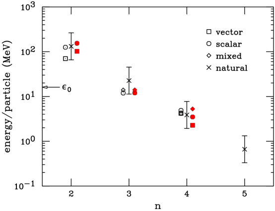
FIG. 4.: Contributions to the binding energy of equilibrium nuclear matter from terms of the form $\rho_{s}^{i}\rho_{v}^{j}$ with $i+j=n$. The symbols indicate terms with $i=0$ (squares), $j=0$ (circles), and $i\neq 0$, $j\neq 0$ (diamonds). The unfilled symbols indicate set FZ4 and the filled symbols indicate set FA4. The crosses are estimates based on Eq. (76).

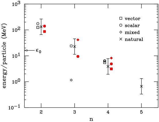
FIG. 5.: Contributions to the binding energy of equilibrium nuclear matter from terms of the form $\rho_{s}^{i}\rho_{v}^{j}$ with $i+j=n$. The symbols indicate terms with $i=0$ (squares), $j=0$ (circles), and $i\neq 0$, $j\neq 0$ (diamonds). The unfilled symbols indicate set VZ4 and the filled symbols indicate set VA4. The crosses are estimates based on Eq. (76).

The implications of naturalness are clear in Figs. 4 and 5, where contributions to the binding energy per nucleon at equilibrium from terms of the form $\rho^{i}_{s}\rho^{j}_{v}$ with $i+j=n$ and $\rho_{v}\equiv j_{v}^{0}$ are plotted for various parameter sets. (The reader is cautioned not to confuse $n$ with the label of the parameter sets associated with the optimal hierarchy). The scale of the natural size of contributions expected from an $n$-th order term is obtained through NDA; since the difference in the scalar and vector densities is small, (the magnitude of) the contribution from such a term can be estimated by

$$\alpha_{\rm nat}\Lambda\left({\rho_{v}\over f_{\pi}^{2}\Lambda}\right)^{n-1}\ ,$$ (76)

where $\alpha_{\rm nat}$ is a (positive) number of order unity and $\rho_{v}$ is the nuclear matter equilibrium density. Estimates for $\Lambda=770\,$MeV are marked in the figures with crosses and the error bars reflect a range of $\alpha_{\rm nat}$ from $1/2$ to 2. We observe that the estimates are quite consistent with the energies found from the fits.

Since the contributions decrease steadily with increasing powers of the densities, the expansion and truncation scheme proposed under NDA is justified. Note that this decrease will become more gradual as the density is increased above equilibrium density. Based on the estimates, a truncation at $n=4$ for ordinary nuclear observables yields an error of order 1 MeV or less. The contributions at fourth-order in the density are on the order of the nuclear-matter binding energy, however, and consistency implies we need to include these terms. In practice, however, the $n=3$ truncation (parameter set P2) is able to absorb the $n=4$ contributions. This result is consistent with a recent analysis of the nonrelativistic Skyrme energy functional [31]. On the other hand, this was not the case in Ref. [9], where the $n=3$ fit, while quite reasonable, was also noticeably inferior to $n=4$.

While the expansion and truncation scheme is supported by our results, a comparison of the various parameter sets shows significant variation for individual parameters. In many cases even the sign is indeterminate. Thus the parameters in this approach, as in the relativistic meson model, are underdetermined. On the other hand, Table VI shows that the optimal parameters are much better constrained by the data. Therefore reformulating the effective theory in terms of an optimal basis may be more productive.

C Equivalent meson masses and Yukawa couplings

No restrictions were imposed during optimization on the signs of the coefficients $\kappa_{2}$, $\zeta_{2}$, and $\xi_{2}$ nor on $\kappa_{d}$, $\zeta_{d}$, and $\xi_{d}$ when they were allowed to vary (the “V” sets). On the other hand, as shown in Tables II–V, a direct transformation from a relativistic mean-field meson model would predict definite signs for these coefficients; the coefficients determined through this transformation would depend only on the squares of the Yukawa couplings, $g_{i}^{2}$, as well as the squares of the meson masses, $m_{i}^{2}$. Sets FA$n$ and FZ$n$ all have positive values for the corresponding values of $g_{i}^{2}$ as well as for the scalar mass squared. (Recall that the corresponding values of $m_{v}$ and $m_{\rho}$ were held fixed for these sets). Parameters sets VZ$n$ and VA$n$, however, include sets with $m_{i}^{2}<0$ and $g_{i}^{2}<0$. The ratio $g_{i}^{2}/m_{i}^{2}$, which is the integrated strength in each channel, is reasonably well determined and is in every case positive.

The difficulty with predicting individual masses and couplings is revealed by Table VI. While $\widetilde{\Delta}_{1}$ is well determined and consistent across the parameter sets, $\widetilde{\Delta}_{2}$ is poorly determined. Thus, the individual values for $\widetilde{\kappa}_{d}$ and $\widetilde{\zeta}_{d}$ are also poorly determined, and we cannot reliably extract masses and couplings from the fits. We conclude that the nuclear observables we have used do not provide sufficient constraints to definitively test whether the point couplings are dominated by an underlying meson phenomenology. The combinations that are well determined correspond to the strength and range of the effective central potential. Specifically, if the static nonrelativistic potential in momentum space from the exchange of scalar and vector mesons is written as:

$$V({\bf q})=4\pi\left(-{g_{s}^{2}\over m_{s}^{2}+{\bf q}^{2}}+{g_{v}^{2}\over m_{v}^{2}+{\bf q}^{2}}\right)\ ,$$ (77)

and expanded in powers of ${\bf q^{2}}$,

$$V({\bf q})=4\pi\left(-{g_{s}^{2}\over m_{s}^{2}}+{g_{v}^{2}\over m_{v}^{2}}\right)-4\pi{\bf q^{2}}\left(-{g_{s}^{2}\over m_{s}^{4}}+{g_{v}^{2}\over m_{v}^{4}}\right)+\cdots\ ,$$ (78)

the two combinations of couplings and masses in parentheses are reasonably well determined.

VII Summary

The successful application of EFT concepts to mean-field mesonic models of nuclei [9] motivates their application to point-coupling models. Such models describe nuclear interactions through contact terms (in a derivative expansion) in place of meson exchange. In comparison to the large body of work on meson models, the analysis of relativistic point-coupling models has been quite limited. Here, we extend the model of Nikolaus, Hoch, and Madland [18] and its analysis by Friar et al. [19] to encompass a more complete analysis based on EFT concepts.

The lagrangian is consistent with the symmetries of QCD and is organized according to the same principle of naive dimensional analysis (NDA) applied to the relativistic meson model of Ref. [9]. The organization is an expansion in powers and derivatives of the densities in ratio to scales dictated by NDA results: a given term in the lagrangian takes the form

$$c\left[\left({\partial\over\Lambda}\right)^{p}\left({\overline{N}\Gamma N\over f_{\pi}^{2}\Lambda}\right)^{l}\right]$$ (79)

where $c$ is a dimensionless coefficient and $p$ and $l$ are integers. (Electromagnetic interactions will also contain a power of the photon field and the electric charge). In principle, all terms consistent with the symmetries should be included to a given order in the expansion, but in the present work we have omitted a variety of terms that we expect to be poorly determined based on meson exchange phenomenology and experience with relativistic meson mean-field models.

The NDA organization provides a valid expansion scheme provided the coefficients are “natural” (on the order of unity); one can construct an energy functional in powers of densities and their derivatives and truncate at some finite order with a controlled error. Our fits to bulk nuclear properties show this to be the case. Beyond a second-order truncation, the models resulting from these fits reproduce the experimental data quite well. We conclude that NDA and the naturalness assumption are compatible with and implied by the observed properties of finite nuclei, even though many-body effects are absorbed into the coefficients.

Point-coupling models therefore provide an alternative phenomenology to mean-field meson models. In principle, a direct transformation exists between any point-coupling and meson mean-field model. The equations of motion for the mean meson fields can be iterated to solve the fields as an expansion in scalar and vector densities. The delicate cancellations at low order in the expansion result in too large a truncation error for such transformations to be of use, however, and any point-coupling model derived from a mesonic model in this way must be refit to the data. We note that naturalness of the point-coupling model was found in the absence of counting factors that were required in the meson model analysis.

Although fourth-order terms would be required for a consistent truncation, a truncation at third order in the point-coupling model can yield a good fit to data, in contrast to the meson models where fourth-order terms were necessary in obtaining a good fit. Due to improvements in the optimization procedure over that used in Ref. [9] through a reorganization of the lagrangian in terms of “optimal parameters”, a true comparison cannot be made until the fits obtained in that reference are reanalyzed.

The analysis in terms of optimal parameters suggests that they may provide a more efficient basis for an expansion. While the individual coefficients in the covariant point-coupling model are in general poorly determined by the nuclear data, the lower-order optimal parameters are quite well constrained and only the highest-order parameters are badly underdetermined. The use of optimal parameters was suggested by methods of the heavy baryon formulation of chiral perturbation theory, adapted to finite density. Further development of this approach and its relation to nonrelativistic energy functionals for nuclei is in progress.

REFERENCES

• [1] S. Weinberg, Physica A96 (1979) 327.
• [2] H. Georgi, Ann. Rev. Nucl. Part. Sci. 43 (1993) 209.
• [3] G. P. Lepage, in From Action to Answers (TASI-89), eds. T. DeGrand and D. Toussaint (World Scientific, Singapore, 1993) p. 483.
• [4] G. Ecker, The Standard Model at Low Energies, from: Lectures given at Sixth Indian-Summer School on Intermediate Energy Physics in Prague, August 1993.
• [5] S. Weinberg, The Quantum Theory of Fields, vol. I: Foundations (Cambridge University Press, New York, 1995).
• [6] D. Kaplan, Effective Field Theories, from: lectures given as Seventh Summer School in Nuclear Physics at the Institute for Nuclear Theory, June 1995.
• [7] J. Gasser and H. Leutwyler Ann. Phys. (NY) 158 (1984) 142; Nucl. Phys. B250 (1985) 465, 517, 539.
• [8] V. Bernard, N. Kaiser, and U. G. Meissner, Int. J. Mod. Phys. E4 (1995) 193.
• [9] R. J. Furnstahl, B. D. Serot, and H.-B. Tang, Nucl. Phys. A615 (1997) 441.
• [10] B. D. Serot and J. D. Walecka, Adv. Nucl. Phys. 16 (1986) 1.
• [11] B. D. Serot and J. D. Walecka, Int. J. Mod. Phys. E (1997), in press.
• [12] A. Manohar and H. Georgi, Nucl. Phys. B234, (1984) 189.
• [13] H. Georgi, Phys. Lett. B298 (1993) 187.
• [14] R. M. Dreizler and E. K. U. Gross, Density Functional Theory (Springer, Berlin, 1990)
• [15] C. Speicher, R. M. Dreizler, and E. Engel, Ann. Phys. (N.Y.) 213 (1992) 312
• [16] R. N. Schmid, E. Engel, and R. M. Dreizler, Phys. Rev. C 52 (1995) 164
• [17] E. Engel, H. Müller, C. Speicher, and R. M. Dreizler, in NATO Advanced Science Institute Series B, vol. 337, eds. E. K. U. Gross and R. M. Dreizler (Plenum, New York, 1995).
• [18] B. A. Nikolaus, T. Hoch, D. G. Madland, Phys. Rev. C 46 (1992) 1757.
• [19] J. Friar, D. G. Madland, B. W. Lynn, Phys. Rev. C 53 (1996) 3085.
• [20] J. L. Friar, Few Body Syst. 99 (1996) 1.
• [21] R. Machleidt, Adv. Nucl. Phys. 19 (1989) 189.
• [22] J. J. Sakurai, Ann. Phys. 11 (1960) 1;
M. Gell-Mann, D. Sharp and W. Wagner, Phys. Rev. Lett. 8 (1962) 261;
• [23] G. E. Brown, M. Rho, and W. Weise, Nucl. Phys. A454 (1986) 669.
• [24] H. de Vries, C. W. de Jager and C. de Vries, At. Data Nucl. Data Tables 36 (1987) 495.
• [25] R. K. Bhaduri, Models of the Nucleon, (Addison Wesley, New York, 1988).
• [26] R. J. Furnstahl, B. D. Serot, and H.-B. Tang, Nucl. Phys. A598 (1996) 539.
• [27] V. Bernard, N. Kaiser, J. Kambor and U. Meisner, Nucl. Phys. B388 (1992) 315.
• [28] E. Jenkins and A. V. Manohar, Phys. Lett. B255 (1991) 558.
• [29] F. James and M. Roos, CERN Program lib. entry D 506 (CERN, Geneva, 1989).
• [30] R. J. Furnstahl, B. D. Serot, and J. J. Rusnak, in preparation.
• [31] R. J. Furnstahl and J. C. Hackworth, Ohio State Preprint nucl-th/9708018, (to appear in Phys. Rev. C).