On the extraction of electromagnetic properties of the (1232) excitation from pion photoproduction
Abstract
Several methods for the treatment of pion photoproduction in the region of the resonance are discussed, in particular the effective Lagrangian approach and the speed plot analysis are compared to a dynamical treatment. As a main topic, we discuss the extraction of the genuine resonance parts of the magnetic dipole and electric quadrupole multipoles of the electromagnetic excitation of the resonance. To this end, we try to relate the various values for the ratio of the E2 to M1 multipole excitation strengths for the resonance as extracted by the different methods to corresponding ratios of a dynamical model. Moreover, it is confirmed that all methods for extracting resonance properties suffer from an unitary ambiguity which is due to some phenomenological contributions entering the models.
pacs:
PACS numbers: 13.60.Rj, 13.60.Le, 14.20.Gk, 25.20.LjI Introduction
One of the most prominent manifestations of internal nucleon structure is the (1232) resonance which is seen, e.g., in pion scattering and electromagnetic (e.m.) pion production. Thus it is not surprising that a large number of experimental and theoretical investigations has been devoted to the understanding of the structure of this resonance. Recently, the question of the relative strength of the electric quadrupole (E2) to the magnetic dipole (M1) excitation in the e.m. transition has become one of the central questions and is subject of numerous papers [1, 2, 3, 4, 5, 6, 7, 8]. While the M1 strength in the simplest approach is directly related to the magnetic properties of the constituents, the E2 strength may be interpreted as a measure of internal spatial deformation, i.e., as deviation of the orbital wave functions from spherical symmetry. Thus, there is considerable experimental effort to provide accurate data on pion photo- and electroproduction from the nucleon in the resonance region [9, 10]. Various methods have been proposed in the literature for the isolation of the genuine resonant part of the experimentally measured multipoles which, however, give quite different answers [1, 3, 11, 12, 13].
The general problem of such an extraction lies in the fact that the experimentally observable multipoles contain important background contributions which cannot be separated in a simple and unique way, so that in most explicit evaluations a specific model is used. Thus it is not surprising that the different prescriptions result in different values of resonance properties. In fact, for photoproduction the values for , the ratio of electric quadrupole to magnetic dipole, vary between to (see e.g. the discussion in [4]). However, in view of the various methods used, it remains unclear how these values should be compared to each other. In other words, is there a common basis for a meaningful comparison?
It is the purpose of this paper to address this question in greater detail. To this end we will compare three different methods which have been recently applied. They are based on (i) a dynamical model (DM) for the coupled N--N system, (ii) the effective Lagrangian approach (EL), and (iii) the recently proposed speed plot analysis (SP). We will take the DM as a common point of reference for this study.
To this end we briefly review in Sect. II the treatment of pion photoproduction based on a dynamical model. Special attention is paid to the general structure of the pion nucleon scattering and photoproduction amplitudes and the implication of unitarity. Sect. III collects the basic formulas of the treatment of these reactions in the framework of ELs, and the connection between quantitities like resonance mass, coupling constants of the ELs and the corresponding quantities of a DM is derived. Moreover, a numerical comparison is performed. In Sect. IV we briefly discuss the SP and point out some shortcomings in the present application and how they can be avoided. The paper ends with a summary and some conclusions.
II Dynamical model
There are two main advantages of treating e.m. pion production dynamically, i.e., solving for a given interaction the corresponding Lippman-Schwinger equation. First of all, it ensures that all two-body unitarity constraints are automatically respected. Secondly, it provides a well defined basis for the analysis of the role of the final state interaction in the e.m. reaction. In such a dynamical approach the model parameters are usually adjusted in order to reproduce all available on-shell data. At present the main disadvantage lies in the fact that a dynamical model requires still some purely phenomenological input, e.g., form factors in order to regularize the driving terms of the interaction, which is essential to solve the dynamical equations. Further problems are related to the neglect of three-body unitarity above two-pion threshold and to the requirements of relativity and gauge invariance. However, various improvements have been achieved recently [11, 13, 14, 15, 16]. Notwithstanding these shortcomings, such a dynamical model still provides the most satisfactory and comprehensive description.
We shall first briefly review the salient features of a dynamical model for the coupled N--N system following the notation of [1, 5]. The Hilbert space is assumed to be a direct sum of bare , and states with corresponding projectors , , and . The Hamiltonian is taken as
| (1) |
with a background interaction , the vertex , a nonresonant driving term , and the vertex . One should note that the energy in the sector depends on the bare resonance mass which is a model parameter to be fitted.
Within such a model the elastic scattering amplitude can be split into a background term and a resonant part
| (2) |
The background term is defined by the integral equation
| (3) |
with the bare propagator . The resonant part
| (4) |
is determined by the dressed and vertices
| (5) |
and the dressed propagator , obtained from
| (6) |
with the free propagator and the self energy
| (7) |
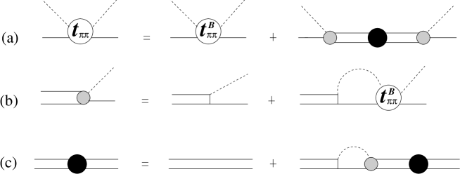
The equations (2) and (4)-(6) are illustrated diagrammatically in Fig. 1. We have already mentioned the fact that the driving terms of the background and resonance amplitudes contain at present phenomenological ingredients which are fitted to the experimental data. Thus these amplitudes and the corresponding phases are to some extent model dependent. Recently we have shown that this model dependence can be interpreted as different, unitarily equivalent representations, yielding different splittings into background and resonant amplitudes but leaving the total amplitude unchanged [5].
The structure of the photoproduction amplitude
| (8) |
is completely analogous. It again splits into a background , determined by
| (9) |
and a resonant part
| (10) |
referred to as “dressed” resonant amplitude. It contains the dressed vertex
| (11) |
Accordingly, one may split further into the so-called bare resonant part and a vertex renormalization , i.e.,
| (12) |
where
| (13) |
and
| (14) |
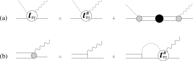
The diagrammatic representation of is shown in Fig. 2. It is obvious that for both multipole amplitudes the same formal structure holds.
The form of the amplitude as discussed above is quite general below the production threshold. In that energy regime, the coupling to the closed channel may be effectively incorporated into a real, energy dependent background interaction, where the energy dependence arises through the energy dependence of the propagators in the intermediate states. Note that such an energy dependence is already introduced by considering the crossed nucleon pole term as background mechanism in the (3,3) channel.
We turn now to the discussion of the basic relations between on-shell matrix elements and phase shifts. In order to avoid a new notation, we will understand all amplitudes in connection with the phase shifts as the corresponding on-shell quantities. For scattering, the scattering amplitude reads
| (15) |
with a phase space factor determined by the adopted normalization conventions, i.e., the scattering matrix is given by
| (16) |
The usual choice is , where denotes the on-shell momentum of the pion in the c.m. frame. Since the background is unitary by itself, one can define a nonresonant background phase shift by
| (17) |
One then easily deduces for the resonant part
| (18) |
where the resonance phase shift is given by
| (19) |
Here we have introduced the dressed mass
| (20) |
Neglecting small Compton scattering corrections [17], Watson’s theorem states that the phase of the photoproduction amplitude below the two pion threshold is given by the hadronic scattering phase shift , i.e.,
| (21) |
where is real. Similarly, one has for the background contribution
| (22) |
with the scattering background phase shift and a real . It is convenient to define an additional phase , called photoproduction background phase [1], so that
| (23) |
where again is real. One should keep in mind that this phase is in general different for the different multipole amplitudes. Moreover, is determined by the elementary interaction model. In detail, one has
| (24) |
For the comparison with the ELs it is useful to express the modulus of the total photoproduction amplitude in terms of the modulus of the resonance amplitude and the photoproduction background phase
| (25) |
Furthermore, for the moduli of the background and bare resonance amplitudes, one easily finds the following relations
| (26) | |||||
| (27) |
Note that the bare amplitude carries the full phase (see (13)). An expression, alternative to (25), is then
| (28) |
which exhibits the resonance and background contributions to .
At the end of this brief review, we collect different possible definitions of ratios for the transition. The ratio of the full amplitudes
| (29) |
is directly related to the experimentally observable multipoles which, according to Watson’s theorem, is a real but energy dependent quantity. The bare ratio
| (30) |
is also a real number because the bare amplitudes carry the total phase as mentioned above. It is directly related to the ratio of the strengths of the coupling constants in the transition current and thus is energy dependent only if the coupling is energy dependent.
With respect to the ratio of the dressed multipoles, one may define two different quantities, since the dressed multipoles carry different phases, namely the complex quantity
| (31) |
or, alternatively, the ratio of the moduli
| (32) |
As we will see in the next Section, this latter quantity is closely related to defined in the EL. Note, that both dressed ratios are energy dependent.
III Effective Lagrangian approach and unitarization methods
Let us first summarize the treatment of pion scattering and pion photoproduction in the effective Lagrangian approach (EL). Here, only the lowest order tree level Feynman diagrams are considered including background and resonance contributions. Subsequently, the resulting amplitude is unitarized. Three different prescriptions for unitarization have been proposed in the literature, the Olsson method [18, 19], the Noelle method [20] and the K-matrix approach [3]. The dependence of the photoproduction process on the adopted unitarization scheme has already been extensively studied by Davidson, Mukhopadhyay and Wittman [3], and we follow their notation for convenience.
We start by collecting the basic formulas for pion nucleon scattering in the energy region of the resonance. The different unitarization methods can be parametrized by the following relation for the phase shift
| (33) |
where is given by the nonresonant tree diagrams. The quantity is interpreted as the -channel contribution of the resonance and parametrized in the form
| (34) |
where the constant mass is obtained as the zero of . The parameter in (33) distinguishes the different unitarization methods, i.e., refers to the Noelle, K-matrix and Olsson approach, respectively. Obviously, all methods coincide in the case of a vanishing background phase shift . For the decay width, the following ansatz is used
| (35) |
where and denote respectively the pion momentum and the nucleon energy in the rest frame. Furthermore, a weak energy dependence of the coupling constant is allowed for
| (36) |
with free parameters and . The background phase shift is parametrized as
| (37) |
with free parameters and to be fitted as well.
In order to establish the connection between the EL and the DM one just has to cast of the DM into a form which corresponds to (33) in terms of the corresponding dynamical quantitities. A straightforward calculation gives
| (38) |
with
| (39) |
where is given in (19).
Equating now (38) with (33), one can express as function of the DM variables and , the EL background phase and the unitarization parameter
| (40) |
By means of Eq. (34), the EL quantitities and can be expressed through DM quantities. In addition, they will also depend on the EL background phase and the unitarization parameter . For example, one finds for the resonance mass parameter
| (41) |
where the right hand side is to be taken at and the dressed energy dependent mass is defined in (20). The dependence on both the EL background phase and the DM background phase reflects the representation dependence mentioned above in the discussion of the DM.
If now we assume the same representation, i.e., identify the background phases , then the expressions simplify considerably, yielding
| (42) | |||||
| (43) |
This is an implicit equation for the mass in the respective unitarization scheme. One has in detail
| (44) | |||||
| (45) | |||||
| (46) | |||||
| (47) |
It is easily seen that in the case of the K-matrix method, corresponds to the energy at which the full phase shift is equal to . Note that the sign of is not fixed a priori. For the model B of Tanabe and Ohta, upon which our later comparison is based, one obtains a negative sign and thus within this model (Olsson) (K-matrix) (Noelle).
Turning now to pion photoproduction, we begin with a brief summary of the treatment of this process as given in [3]. In the EL, one starts from the tree level contributions of background and resonance terms
| (48) |
For our purpose, it is not necessary to specify the explicit expressions for the real numbers and , which are given in [3]. The unitarized amplitude then has the form
| (49) |
with
| (50) |
The real amplitude and the photoproduction background phase are functions of , and the phases and whose explicit form depends on the unitarization method and which will be given below. The ratio is then given in terms of the appropriate electric and magnetic amplitudes defined correspondingly as in (48)
| (51) |
In the literature, the ratios (EL) are quoted just at the energy of the respective unitarization scheme.
Now we can establish the relations between the EL amplitudes and the DM quantities on the basis that the total phase shift and the total multipole amplitudes can be identified, i.e., give a satisfactory fit to experimental data. In Olsson’s method, the unitarized amplitude is given in the form
| (52) |
with
| (53) |
leading to the correspondence . As already pointed out by Olsson [18], no solution arises in the case when , as is the case for the excitation of the . This problem is avoided, when the helicity amplitudes are unitarized instead of the multipoles [3]. However, this trick would not work in the case of a weak resonance which is produced by one e.m. multipole only. The comparison with the DM, which has already been performed by Tanabe and Ohta [1], is based on the identification of (50) with (25). It yields the following relation
| (54) |
It is worth noting that, when identifying the respective background contributions in EL and DM, the case cannot appear, because in the dynamical model the photoproduction background phase is a well defined quantity. Although this relation between and the dressed amplitude depends also on the various phases of DM and EL and thus does not allow a simple interpretation, one sees that the ratio is just the ratio of the moduli of the dressed multipoles in the DM (see (32))
| (55) |
In Noelle’s scheme, the unitarized amplitude is given by
| (56) |
which leads to the following expressions
| (57) | |||||
| (58) |
The connection between and the DM amplitudes reads
| (59) |
Due to the explicit appearance of the background contributions, there is again no simple interpretation for in terms of the dynamically calculated quantities. On the other hand, the ratio becomes quite simple
| (60) |
Obviously, there is no simple relation between this ratio and the dynamical resonance parameters. However, if one evaluates this ratio at , one finds
| (61) |
In the K-matrix approach, one identifies the tree level contributions as K-matrix elements. The full unitarized photoproduction amplitude reads then
| (62) |
Since here the following relation holds
| (63) |
one finds
| (64) |
Comparing (64) with (56) one finds the following relation
| (65) |
which immediately leads to the same energy dependent for the K-matrix as in Noelle’s approach, and thus in the K-matrix approach the ratio quoted in the literature is nothing else than the ratio of the experimental multipoles at .
We close this Section by comparing the explicit numerical values for the various ratios and other quantities introduced above with the dynamical model of Tanabe and Ohta (model B in [1]). From their model one deduces from Eqs. (46)-(45) the following masses: , and . The ordering of the masses is due to the negative self-energy contribution of this model. It turns out, that the values obtained in this manner are not far away from the numbers quoted in [3], which are MeV, MeV, and MeV, respectively. The small difference in the K-matrix method has its origin in the fact that different data for had been fitted in both papers [1, 3].
As next we calculate on the basis of the DM the coupling “constant” for the different ELs via the decay width given in (35) using Eqs. (34), (42) and (43). The result is shown in Fig. 3. One readily notices a 15 percent variation of the coupling strength between Olsson and K-matrix method. Furthermore, the energy dependence, which can be traced back to the energy dependence of the self-energy in the DM, is rather weak and similar for all three schemes but not negligible at all. At least for the simple model of Tanabe and Ohta, it is larger than the energy dependence allowed for by Davidson et al. [3].
In Fig. 4 we show the various E2/M1 ratios as a function of the photon lab energy. There are basically three different dressed ratios, (Olsson), , and (K-matrix). Note that these identifications are based on the assumption that the background contributions, which may formally be obtained by putting in DM and EL, can be identified. The difference between the ratios is obvious. In particular, comparing (Olsson) with , one readily notes quite a distinct different energy dependence, while (K-matrix) behaves qualitatively similar as , although differences remain in detail. If evaluated at the respective masses , we find %, % and %. The difference to the results of [3] can be traced back mainly to different prescriptions for the e.m. and hadronic background contributions. Since all ratios are based on the same DM, these different results clearly reflect the fact that a meaningful comparison is not possible. In this context we recall that except for (K-matrix), the dressed ratios are representation dependent.
IV Speed plot analysis
The essential idea of the speed plot analysis (SP) rests on the analytic properties of the partial wave amplitude. A resonance manifests itself as a pole in the lower half plane of the second Riemann sheet when continuing the amplitude into the complex energy plane. The aim of the SP is to locate the pole position and to determine the corresponding residue from the experimental data. This method, originally used in pion scattering, has been applied very recently to pion photoproduction by Hanstein, Drechsel and Tiator [12]. Assuming a well isolated pole for the resonance, one can separate it by performing a Laurent expansion in the vicinity of the pole, resulting in the form
| (66) |
with the pole term
| (67) |
and the regular part
| (68) |
with constant complex coefficients . Here, denotes the pole position with constant resonance mass and width , and and characterize modulus and phase of the residue.
If we apply this analysis to the DM, the pole is determined as solution of
| (69) |
on the second Riemann sheet, which leads to a sytem of coupled equations for the resonance mass and width
| (70) | |||||
| (71) |
Expanding then the DM amplitude as in (66), one immediately sees that the splitting into a pole and a regular part formally is not identical with the splitting into a resonance and a background part because of an additional energy dependence of the dressed resonance amplitude besides the pole contribution.
However, this formal criticism may not be too relevant in the actual application if the background amplitude is very weakly energy dependent. To this end, let us first briefly review the SP of elastic scattering as performed by Höhler [21, 22] to determine the resonance pole parameters (, ). It is based on the following parametrization of a resonant partial wave amplitude by splitting it into a background and a pole part
| (72) |
where
| (73) |
with
| (74) |
Since the resonance lies in the elastic region, Höhler’s parametrization requires in addition separate unitarity for the background. Thus a real phase shift can be assigned by
| (75) |
As discussed in Sect. II, Eq. (75) is a natural consequence in any dynamical model. In the elastic region, of course, also the full amplitude is unitary,
| (76) |
which fixes the quantity
| (77) |
Assuming (and thus and ) to be energy independent, one can extract the pole parameters and directly from the speed of the full amplitude, which is defined as
| (78) |
Then one finds from (72)
| (79) |
Thus the maximum of the speed is located at , determining the resonance mass. Furthermore, the width is then obtained from the half maximum values
| (80) |
or from the curvature at maximum speed
| (81) |
The latter should be preferred for a broad resonance but might be more difficult to evaluate numerically. Höhler [21] finds
| (82) |
These values may be used to calculate from (72) for the whole energy range and to check the initial assumption with respect to the energy dependence of . Indeed, one finds at resonance and only a very small variation of with energy which justifies the method. An important point to note so far is that and in Höhler’s analysis may well be considered as approximations to background and dressed amplitudes and of a certain dynamical model in a limited energy intervall around the resonance position. In view of the fact that one can generate a whole family of phase equivalent dynamical models by means of unitary transformations without changing the pole position in the complex plane, one may conclude that the speed plot analysis singles out from this family the one which predicts a dressed amplitude that is most accurately approximated by its pole term and which gives the weakest energy dependence of the background . On the mass shell, it would provide dynamical amplitudes and which are closest to Höhler’s amplitudes and , respectively. This observation could also provide a possible explanation for the fact that the resulting background phase is repulsive in contrast to standard attractive background interactions as has been noted already by Höhler [22].
The recent extension of the SP to pion photoproduction by Hanstein et al. [12] takes as starting point the following ansatz for the photoproduction amplitude
| (83) |
where is the photoproduction Born amplitude calculated from the pseudoscalar Lagrangian. Assuming to be energy independent, they could determine the pole parameters , and the residue from the speed of the difference between the full and the Born amplitude,
| (84) |
The main reason for critisizing this procedure is two-fold: (i) In the original SP of scattering [21, 22] Born terms have not been subtracted, i.e., the speed of the full amplitude determines the pole parameters. Moreover, only the speed of the full amplitude is related to the time delay between the arrival of the incident wave packet at the collision region and the departure of the outgoing packet. (ii) There is no reason to give up the separate unitarity constraint for the background amplitude and to treat the hadronic and e.m. reactions in a different manner.
Therefore, we propose as a consequent extension of Höhler’s ansatz (72) to e.m. pion production in the elastic region the form
| (85) |
where again it is assumed that the background term obeys itself the unitarity constraint, i.e., it fulfills Watson’s theorem which implies that is real. The constraint from Watson’s theorem for the full amplitude , which can be written as
| (86) |
finally allows to eliminate the unknown modulus of the background amplitude in Eq. (85). One finds
| (87) |
Of course, the information contained in (85) and (87) is not sufficient to fix the complex function over a larger energy range from available experimental multipole data sets. However, it allows to check whether the data can be described at all over a limited energy range around the resonance position replacing by the residue .
We have performed such a SP taking as input “data” the multipoles from the fixed- dispersion analysis of Hanstein et al. [12]. By construction, these multipoles exactly obey Watson’s theorem, and thus they provide at the same time a “data” set for the scattering phase shift . Writing the residue , it is obvious (see (85) and (87)) that its modulus is given by the ratio of the speeds of the hadronic and e.m. amplitudes
| (88) |
This ratio is plotted as a function of the energy in the left panel of Fig. 5. The plateau around already indicates that the assumption of a constant residue may provide a good approximation in an energy interval around the resonance position. The phase of the residue can be calculated from the relation
| (89) |
which follows directly from (85) and (87). Our values for are compared with the ones of Ref. [12] in Table I. In the case of the electric multipole , both values agree very well. However, a somewhat larger deviation is found for . For the ratio of the residues of electric to magnetic multipoles we obtain
| (90) |
Comparison to the result of [12] shows a good agreement for the imaginary part while the real part is 10 percent smaller.
Most of the difference between the approach of Hanstein et al. and ours can be traced back to the phase of the background of the magnetic multipole. Whereas in our ansatz the phases of both background amplitudes agree by definition with , which is already fixed in the analysis of scattering, the phase of the background in (83) is unconstrained since is an arbitrary complex number. As shown in Fig. 6, they differ even in sign for both multipoles. Only the electric background phase (dotted curve) is close to (solid curve). Consequently, the background and pole terms found in [12] cannot, even approximately, be identified with the background and dressed multipoles and , respectively, of any dynamical model. However, this is possible for our results in the approximate way discussed above. Fig. 7 shows the quality of the pole approximation, i.e., evaluating (85) with , in comparison with the full multipoles. Clearly, the pole approximation cannot reproduce the data below and above the resonance region as it not need to. In particular, it is obvious that by definition the pole approximation leads to a wrong low-energy behaviour.
There remains one final point to be mentioned. It concerns the proper normalization of the amplitude for which the speed is calculated since any energy dependent normalization factor would affect the result. According to [22], two times the speed of the -matrix (which is related to the -matrix through ) defines the quantity which can be interpreted as a time delay. This suggests to study the speed of the product of times the multipole, where and are the c.m. momenta of pion and photon, respectively. (The relation between -matrix and multipoles can be found e.g. in [17]). Since in the resonance region, this factor is not negligible. We have performed this modified speed analysis (mSP), i.e., identified in Eq. (85) with times the multipole, instead of taking the multipole itself as before and in Ref. [12]. The results are summarized in Fig. 5 (right panel) and Table I (middle column). In order to allow a direct comparison with the foregoing SP, we present the mSP results in terms of where and are the momenta at . From Table I one obtains
| (91) |
which differs significantly from in (90). In addition, we have checked that the quality of the pole approximation, which can be achieved within the mSP, is very similar to the one shown in Fig. 7.
This last point shows the following: Without reference to the physical interpretation of the speed in terms of the above mentioned time delay, one would not have an unique prescription for the choice of the amplitude for which the speed should be calculated and thus the whole procedure would become rather ambiguous.
V Summary and conclusions
We have analyzed in detail different theoretical descriptions of pion photoproduction in the region of the resonance, namely, dynamical models, effective Lagrangian approaches, and the recently proposed speed plot analysis. Our main emphasis has been laid on the question to what extent genuine resonance contributions to the e.m. multipoles can be extracted, in particular, the interesting and controversely discussed E2/M1 ratio for the e.m. excitation.
As theoretical basis we have chosen a dynamical model for which we have briefly reviewed the treatment of pion nucleon scattering and pion photoproduction, in particular the separation of background and resonance properties. For the Effective Lagrangian approaches, we have discussed the different unitarization schemes resulting in different background and resonance contributions as pointed out already in [3]. It turns out that a priori there is no direct relation of background and resonance contributions of a DM to the corresponding ones of a EL. The main reason for this is that unitarity is put in by hand in the EL which does not allow the identification of the background part. Only on the premises that the hadronic background phases could be identified, the various resonance parameters like resonance mass, decay width, and E2/M1 ratio could be related. This reflects the fact, that the largely phenomenological treatment of the background introduces a unitary ambiguity or representation dependence [5]. Therefore, almost all E2/M1 ratios discussed so far are representation dependent quantities which implies that they are not observable in the strict sense. There is one exception, namely the ratios in the Noelle and K-matrix approach, when evaluated at the resonance position, because they are simply given by the ratio of the full multipoles at this energy.
The main problem, however, how these numbers should be compared to a given microscopic hadron model, remains unresolved. The only safe solution is to calculate the complete pion production amplitude within such a model in order to have an unambiguous and direct comparison to experimentally observable quantities.
As last topic, we have studied the recently proposed speed plot analysis of Hanstein el al. We could show that the separated resonance and background contributions of their analysis cannot be identified with corresponding DM quantities, since their ansatz for the background is not constrained by unitarity. For this reason, we have proposed an alternative speed plot analysis which respects the separate unitarity condition for the background. In such an analysis, the regular and pole contributions can be viewed as approximations of the background and dressed resonant contribution of a certain dynamical model. Applied to the same input as Hanstein et al., we find a similar result for the residue of the electric multipole, whereas differences of the order of 10 percent appear for the magnetic multipole. Accordingly, we obtain a slightly changed ratio . In addition, we have proposed a further modification of the speed analysis which was guided by the physical interpretation of the speed in terms of the time delay between incoming and outgoing wavepackets. This modification leads to a 20 percent change in the ratio. But again it remains unclear how could be compared to any microscopic hadron model.
Even though we have focused here on the , the conclusions are also valid for the case of electroexcitation and/or the excitation of higher resonances. In the latter case, the situation is even worse due to overlapping resonances and the coupling to many pion channels, which makes a realistic dynamical calculation more difficult.
Acknowledgements
We thank R. Beck and A. M. Bernstein for many fruitful discussions. This work was supported by the Deutsche Forschungsgemeinschaft (SFB 201).
REFERENCES
- [1] H. Tanabe and K. Ohta, Phys. Rev. C 31, 1876 (1985).
- [2] S. N. Yang, J. Phys. G 11, L205 (1985).
- [3] R. Davidson, N. C. Mukhopadhyay, and R. Wittman, Phys. Rev. Lett. 56, 804 (1986); Phys. Rev. D 43, 71 (1991).
- [4] A. M. Bernstein, S. Nozawa, and M. A. Moinester, Phys. Rev. C 47, 1274 (1993).
- [5] P. Wilhelm, Th. Wilbois, and H. Arenhövel, Phys. Rev. C 54, 1423 (1996).
- [6] A. J. Buchmann, E. Hernandez, A. Faessler, Phys. Rev. C 55, 448 (1997).
- [7] D. H. Lu, A. W. Thomas, and A. G. Williams, Phys. Rev. C 55, 3108 (1997).
- [8] P. N. Shen, Y. B. Dong, Z. Y. Zhang, Y. W. Yu, T.-S. H. Lee, Phys. Rev. C 55, 2024 (1997).
- [9] G. Blanpied et al., Phys. Rev. Lett. 69, 1880 (1992).
- [10] R. Beck et al., Phys. Rev. Lett. 78, 606 (1997).
- [11] S. Nozawa, B. Blankleider, and T.-S. H. Lee, Nucl. Phys. A513, 459 (1990).
- [12] O. Hanstein, D. Drechsel, and L. Tiator, Phys. Lett. B 385, 45 (1996).
- [13] T. Sato, and T.-S. H. Lee, Phys. Rev. C 54, 2260 (1996).
- [14] F. Gross, and Y. Surya, Phys. Rev. C 47, 703 (1993); Y. Surya, and F. Gross, Phys. Rev. C 53, 2422 (1996).
- [15] C. T. Hung, S. N. Yang, and T.-S. H. Lee, Jour. Phys. G 20, 1531 (1994).
- [16] V. Pascalutsa, and J. A. Tjon, contribution, Few-Body XV (Groningen, 1997), to appear in the conference proceedings.
- [17] M. Benmerouche and N. C. Mukhopadhyay, Phys. Rev. D 46, 101 (1992)
- [18] M. G. Olsson, Nucl. Phys. B78, 55 (1974).
- [19] We would like to recall that in a later paper, M. G. Olsson, Nuovo Cim. 40 A, 284 (1977), Olsson himself criticized the unitarization method of [18] as unorthodox.
- [20] P. Noelle, Prog. Theor. Phys. 60, 778 (1974).
- [21] G. Höhler and A. Schulte, Newsletter 7, 94 (1992).
- [22] G. Höhler, Newsletter 9, 1 (1993).
| present (SP) | present (mSP) | from [12] | |
|---|---|---|---|
| 2.47 | 2.24 | 2.46 | |
| (deg) | 156 | 154.7 | |
| 39.9 | 41.5 | 42.32 | |
| (deg) | 26.0 | 27.5 |