HBT with Space- vs. Time-like Hydrodynamic Freezeout

Abstract

Bose-Einstein correlations in relativistic heavy ion collisions and their dependence on the freeze-out condition in hydrodynamic models is examined. The Cooper & Frye space-like freeze-out mechanism is compared to time-like freeze-out, where particles are emitted away only from the surface, i.e. space- vs. time-like freeze-out. The corresponding HBT radii are calculated for the two models emphasizing the difference in the outward HBT radius.

1 Introduction

Bose-Einstein interference of identical particles or the Hanbury-Brown & Twiss effect (HBT) [1] shows up in correlation functions of pions and kaons emitted from the collision zone in relativistic heavy ion collisions. It is an important tool for determining the source at freeze-out and recent data from relativistic heavy ion collisions can restrict the rather different models, that have been developed to describe particle emission in high energy nuclear collisions. In hydrodynamical calculations particles freeze-out at a hypersurface that generally does not move very much transversally until the very end of the freeze-out [2, 3, 4, 5]. In cascade codes the last interaction points are also found to be distributed in transverse direction around a mean value that does not change much with time [6, 7, 8, 9], but the width of the emission zone increases from narrow surface emission to a widespread volume emission. In the first stage the freeze-out surface is relatively static in the transverse direction and the emission extends in time whereas in the second stage the freeze-out happens relatively rapid all over the spatial extent of the source. The two stages are often referred to as surface and volume freeze-out respectively, or time-like and space-like freeze-out (see Fig. 1).^a The distinction is, of course, only approximate and the amount of particles assigned to the two stages varies between models.

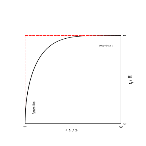
Figure 1: Schematic picture of the transverse position and invariant time of the freeze-out surface in hydrodynamic calculations. The dashed curve approximates the source by time- and space-like components.

In the Cooper & Frye freeze-out assumption the net number of particles leaving the hydrodynamic region is [10]

$${\rm Cooper\,\&\,Frye\,(space-like):}\quad\quad E\frac{dN}{d^{3}p}=\frac{g}{2\pi}\int_{\sigma}d\sigma_{\mu}p^{\mu}f(x,p)\,,$$ (1)

where $f(x,p)=(exp(p\cdot u(x)/T(x)\pm 1)^{-1}$ is the standard thermal Bose or Fermion distribution function with local flow velocity $u(x)$. The freeze-out hypersurface is denoted by $\sigma_{\mu}$ and is usually defined at a constant energy density or temperature $T_{c}\simeq 100-150$ MeV which is determined from the $p_{\perp}$ slopes.

It was pointed by Sinyukov [11] that the Cooper & Frye freeze-out was inconsistent for time-like freeze-out since particles might reenter the hydrodynamic phase. He therefore reflected the momenta in the local rest frame at the boundary for those particles that would have reentered the fluid

$${\rm Sinyukov\,(time-like):}\quad\quad E\frac{dN}{d^{3}p}=\frac{g}{2\pi}\int_{\sigma}d\sigma_{\mu}p^{\mu}f(x,{\cal R}_{\sigma}[p])\,,$$ (2)

where ${\cal R}_{\sigma}[p]$ reflects the component of the particle momentum normal to the freeze-out surface in the local rest frame of the fluid. The argument for doing this was that for each particle reentering there is an outgoing particle inside the fluid that would have escaped into the free streaming region. However, this is not true when the surface is moving (with velocity ${\bf v}_{s}$) in which case slow particles may be overtaken by the freeze-out surface. Defining ${\bf n}_{\sigma}(x)$ as a vector normal to the freeze-out surface and directed away from the fluid and outward into the free streaming phase, the condition for freeze-out is that particle velocities ${\bf v_{p}}={\bf p}/E$ obey

$$({\bf v_{p}}-{\bf v}_{s}(x))\cdot{\bf n}_{\sigma}(x)>0\,.$$ (3)

Particles in the fluid cell to be frozen out that do not fulfill this condition should therefore have their momenta reflected in the frame of the surface. When the surface moves rapidly inwards not many particles need to have their momenta reflected. Likewise, when there is strong outward directed flow the thermal factor $\exp(p\cdot u(x))$ in distribution function automatically guarantees that not many particles move slower than the surface speed. But for small flow and slowly moving surfaces half of the particles should be reflected.

The above prescription for correcting the time-like part of the Cooper & Frye freeze-out assumption may be considered as an improvement. Yet, there are a number of considerations that remain uncured. It should be pointed out that this modified time-like freeze-out assumption preserves momentum and energy globally in the fluid, when it is applied to both sides, but not locally near the surface. At the surface there is a net back reaction due to the surface emission/evaporation that in the time-like freeze-out is away from the surface only. In the treatment of Godunov (see, e.g., [12]) restricting freeze-out to those particle for which the four-vector product, $n(x)\cdot p>0$, is positive does, however, not conserve global energy. Also rescatterings and final state interactions of emitted particles are still ignored. Another issue is the assumption of a sharp freeze-out surface. In reality the freeze-out take place when the particle mean free path becomes long enough that it can escape and the hydrodynamic assumption of a short mean free path breaks down near the surface. This is naturally included in cascade models which find an extended region of final interactions points around what is thus a diffuse surface layer. Recently, Grassi et al. have improved the sharp surface assumption in hydrodynamic models by a Glauber model approach [13] (see also Csernai, these proceedings[3]). Similar ideas have been discussed in [14] in connection with opaque sources emitting from a surface layer of thickness $\sim\lambda_{mfp}$ and their effects on HBT have been calculated.

2 Space-like vs Time-like emission

We will discuss space-time correlations from hydrodynamic sources with the Cooper & Frye (space-like) and Sinyukov (time-like) freeze-out assumption and compare them. In the subsequent chapter we will then consider two-component sources with both space- and time-like emission.

To study the differences between the freeze-out conditions we restrict ourselves to a class of models that have:

i) cylindrical symmetry around the beam or z-axis,^b

ii) longitudinal expansion with Bjorken scaling,

iii) no transverse flow.^c

The distribution of emitted particles also referred to as the source of emission points is with the Cooper & Frye freeze-out assumption

$$S_{CF}(x,p)\sim e^{-p\cdot u(x)/T(x)}\,S_{\tau}(\tau)\delta(r_{\perp}-R(\tau))\,,$$ (4)

Here, the Bjorken variable $\tau=\sqrt{t^{2}-{\rm z}^{2}}$ is the invariant time and $\eta=0.5\ln(t+{\rm z})/(t-{\rm z})$ the space-time rapidity. The flow four-vector is $u=(\cosh(\eta),\sinh(\eta),0,0)$, which gives $p\cdot u=m_{\perp}\cosh(\eta-Y)$. $R(\tau)$ is the transverse radius of the freeze-out surface that moves in time. Initially, when the nuclei collide $R(0)$ is the transverse size of the nuclear overlap zone and final freeze-out takes place when $R(\tau_{f})=0$. The surface speed is $v_{s}=dR(\tau)/d\tau$. The temporal source factor $S_{\tau}(\tau)$ determines the amount of particles that freeze-out per surface element at invariant time $\tau$. Notice that any normalization is irrelevant as they cancel out in later correlation functions (15) and HBT radii.

The Sinyukov freeze-out assumption for a time-like source without flow differ from the Cooper & Frye by

$$S_{S}(x,p)=2\,S_{CF}(x,p)\,\Theta({\bf p\cdot n}_{\sigma}(x))=2\,S_{CF}(x,p)\,\Theta(\cos\theta)\,,$$ (5)

where $\theta$ is the polar angle between ${\bf p}$ and the vector ${\bf n}_{\sigma}(x)$ normal to the freeze-out surface and directed away from the fluid and outward into the free streaming phase. Notice, that the reflection does not change the single particle distribution functions but only correlation functions that are sensitive to correlations between $p$ and $x$.

3 HBT Radii

We follow the standard definition of correlation functions and the HBT radii as is described in more detail in the appendix. It is common to boost longitudinally so that the pair rapidity always is $Y=0$ and choose the direction of ${\bf p}=({\bf p}_{1}+{\bf p}_{2})/2$ along the outward or x direction whereas the third y-direction is called the sideward directions. In cylindrical coordinates we choose the polar angle with respect to the x-axis and so the factor distinguishing the Cooper & Frye from the Sinyukov freeze-out is simply $\Theta(\cos\theta)$.

The HBT radii are for a space-like source $S_{CF}(p,x)$, for which $\langle{\rm x}\rangle=\langle\cos\theta\rangle=0$,

$$R_{l}^{2} \equiv \langle({\rm z}-\beta_{l}t)^{2}\rangle\simeq\langle\tau^{2}\rangle\frac{T}{m_{\perp}}\,.$$ (6)

$$R_{s}^{2} \equiv \langle{\rm y}^{2}\rangle=\frac{1}{2}\langle R(\tau)^{2}\rangle\,,$$ (7)

$$R_{o}^{2} \equiv \langle({\rm x}-\beta_{o}t)^{2}\rangle=\frac{1}{2}\langle R(\tau)^{2}\rangle\,+\,\beta_{o}^{2}\sigma(\tau)\,.$$ (8)

The temporal and angular averages and fluctuations are described in the appendix.

The outward HBT radius is thus larger than the sideward [16, 17]

$$R_{o}^{2}=R_{s}^{2}+\beta_{o}^{2}\sigma(\tau)\,.$$ (9)

The measured out- and sideward HBT radii are very similar in relativistic heavy ion collisions and is based on Eq. (9) taken as an indication of very small duration of emission, i.e., particles appear or freeze-out in a “flash” [19].

Changing the Cooper & Frye freeze-out to that of Sinyukov does not change the sideward and longitudinal HBT radii since the reflection is only in the outward or x-direction. However, the outward HBT radius differ because the reflection has the effect that only particles from the front side of the source pointing towards a given detector are measured in that detector whereas those from the back side are not. The geometry is chosen such that the outward or x-axis is always along the particle momenta ${\bf p}\simeq{\bf p}$ which guaranties that only the half sphere toward any detector is seen in that detector. This has the important consequence that $\langle{\rm x}\rangle$ no longer vanishes but almost cancels $\langle{\rm x}^{2}\rangle^{1/2}$. We find^d

$$R_{o}^{2} \equiv (\frac{1}{2}-\frac{4}{\pi^{2}})\langle R(\tau)\rangle^{2}+\beta_{o}^{2}\sigma(\tau)+\frac{1}{2}\sigma(R(\tau))$$ (10)

$$\,-\,2\beta_{o}\frac{2}{\pi}\langle(R(\tau)-\langle R(\tau)\rangle)(\tau-\langle\tau\rangle)\rangle\,.$$

For a static surface $R(\tau)=constant$ the last two terms vanish; for an inward moving surface the last term is positive. The first term in (10) is $\sigma({\rm x})$ and is significantly reduced as compared to (8). As a consequence Eq. (9) no longer holds as was also found for opaque sources or sources with strong transverse flow [14].

4 Two Component Source

It is important to distinguish between space- and time-like freeze–out, since they give very different HBT radii. Hydrodynamical models [3, 2, 4, 5] assume that particles are emitted from the surface. This is actually also found in some cascade models at early times of the collision [6, 7, 8, 9], but eventually the whole source freezes out and disintegrates. The late stage of cascade models resembles more a volume freeze–out. These sources can approximately be described by two components, initially surface emission but eventually volume freeze-out. Generally, for a two-component source $S(x)=pS_{1}(x)+(1-p)S_{2}(x)$, properly normalized ($\int d^{4}xS_{i}(x)=1$) such that $p$ is the fraction of particles from source 1, the fluctuations in a quantity ${\cal O}$ is from (17)

$$\sigma({\cal O})=p\,\sigma_{1}({\cal O})+(1-p)\,\sigma_{2}({\cal O})+p\,(1-p)\,(\langle{\cal O}\rangle_{1}-\langle{\cal O}\rangle_{2})^{2}\,.$$ (11)

Here, $\langle{\cal O}\rangle_{i}\equiv\int d^{4}xS_{i}(x){\cal O}$ and $\sigma_{i}({\cal O})=\langle{\cal O}^{2}\rangle_{i}-\langle{\cal O}\rangle_{i}^{2}$. The fluctuations are the weighted sum of the fluctuations in the individual sources and an additional cross term. Since $\langle{\rm y}\rangle=0$ and $\langle z-\beta_{l}t\rangle$ also vanishes for $Y=0$ this additional cross term does not contribute to the sideward and longitudinal HBT radii. It is, however, nonnegligible for the outward HBT radius.

Let us approximate the qualitative features of hydrodynamic and cascade models by a toy model with two-components: an approximately static surface $R(\tau)=R$ for times $0<\tau<\tau_{f}$ and a rapid freeze-out of the remaining source at $\tau=\tau_{f}$. The first component violates Eq. (3) for the inward moving particles and is thus time-like for which we should use the Sinyukov freeze-out assumption. The second component is space-like and we should apply the Cooper & Frye freeze-out assumption. We weight the particles frozen-out from the two component by the fractions $p$ and $(1-p)$ respectively. The corresponding HBT radii are found by the expressions (6), (7), (8), and (10) by combining them according to (11)

$$R_{l}^{2} = (1-\frac{p}{2})\tau_{f}^{2}\frac{T}{m_{\perp}}\,.$$ (12)

$$R_{s}^{2} = \frac{1}{4}(1+p)R^{2}\,,$$ (13)

$$R_{o}^{2} = \left((\frac{1}{4}(1+p)-\frac{4}{\pi^{2}}p^{2}\right)R^{2}\,+\,\frac{p}{18}\beta_{o}^{2}\tau_{f}^{2}\,,$$ (14)

Figure 2: Sideward and outward radii as function of the fraction of time-like emitted particles $p$; the amount of space-like emitted particles by the standard Cooper & Frye freeze-out assumption is $(1-p)$. Dashed curves are $R_{0}^{2}/R^{2}$ with freeze-out times of $\beta_{o}\tau_{f}/R=0,1,2$.

In Fig. 2 we show the dependence of the out- and sideward HBT radii on the space- vs. time-like fraction $p$. The freeze-out assumption clearly plays an important role and the difference $R_{o}^{2}-R_{s}^{2}$ is a very sensitive quantity. The fraction of time-like emission $p$ is a model dependent parameter and in reality there will be a gradual transition from time- to space-like emission. Also a finite width of the emission layer [14] will diminish the difference. Transverse flow has a similar effect of directed emission and leads to further reducing $R_{o}$ with respect to $R_{s}$ [14]. However, strong transverse flow $u_{\perp}$ also has the effect of improving the condition of Eq. (3) reducing range of particle velocities for which time-like emission occur.

5 Summary

The validity of Cooper & Frye space-time freeze-out assumption has been discussed. For sources with time-like emission it breaks down and one should rather apply a modified freeze-out assumption like that of Sinyukov which only allows emission away from the fluid. It was shown in a simple toy model that the different freeze-out conditions gave drastically different results for the outward HBT radius. A number of effects such as transverse flow, diffuse surfaces, etc., reduce the difference between the two freeze-out conditions.

In the hydrodynamic calculations of Ref. [5] at RHIC energies the outward HBT radius $R_{o}$ is considerably larger than $R_{s}$. This is mainly due to the existence of a long lived mixed phase of quark-gluon plasma and hadronic matter for the equation of state and initial conditions assumed in this calculation. Thus it is the duration of emission that gives large $R_{o}^{2}-R_{s}^{2}$ or $R_{o}/R_{s}$ and this part is unaffected by changing the freeze-out assumption from Cooper & Frye to that of Sinyukov as can be seen from Eqs. (8) and (10). At AGS and SPS energies, however, the measured $R_{s}$ and $R_{s}$ are very similar excluding the possibility for a long lived mixed phase and the difference arising from the freeze-out assumption may be significant.

Appendix: Correlation functions and HBT radii.

For the correlation function analysis of Bose-Einstein interference from a source of size $R$, we consider two particles emitted a distance $\sim R$ apart with relative momentum ${\bf q}=({\bf p}_{1}-{\bf p}_{2})$ and average momentum, ${\bf p}=({\bf p}_{1}+{\bf p}_{2})/2$. Typical heavy ion sources in nuclear collisions are of size $R\sim 5$ fm, so that interference occurs predominantly when $q\raisebox{-2.15277pt}{$\stackrel{{\scriptstyle<}}{{\sim}}$}\hbar/R\sim 40$ MeV/c. Since typical particle momenta are $p_{i}\simeq p\sim 300$ MeV, the interfering particles travel almost parallel, i.e., $p_{1}\simeq p_{2}\simeq p\gg q$. The correlation function due to Bose-Einstein interference of identical particles from an incoherent source is (see, e.g., [17])

$$C_{2}({\bf q},{\bf p})=1\;\pm\;|\frac{\int d^{4}x\;S(x,{\bf p})\;e^{iqx}}{\int d^{4}x\;S(x,{\bf p})}|^{2}\,,$$ (15)

where $S(x,{\bf p})$ is a function describing the phase space density of the emitting source. The $+/-$ refers to boson/fermions respectively.

Experimentally the correlation functions for identical mesons ($\pi^{\pm}\pi^{\pm}$, $K^{\pm}K^{\pm}$, etc.) are often parametrized by the gaussian form

$$C_{2}(q_{s},q_{o},q_{l})=1+\lambda\exp(-q_{s}^{2}R_{s}^{2}-q_{o}^{2}R_{o}^{2}-q_{l}^{2}R_{l}^{2}-2q_{o}q_{l}R_{ol}^{2})\;.$$ (16)

Here, ${\bf q}={\bf k}_{1}-{\bf k}_{2}=(q_{s},q_{o},q_{l})$ is the relative momentum between the two particles and $R_{i},i=s,o,l$ the corresponding sideward, outward and longitudinal HBT radii respectively. We will employ the standard geometry, where the longitudinal direction is along the beam axis and the outward direction is along ${\bf p}$ and the sideward axis is perpendicular to these. Usually, each pair of mesons is lorentz boosted longitudinal to the system where their rapidity vanish, $Y=0$. Their average momentum ${\bf p}$ is then perpendicular to the beam axis and is chosen as the outward direction. In this system the pair velocity $\beta_{p}$=${\bf p}/E_{p}$ points in the outward direction with $\beta_{o}=p_{\perp}/m_{\perp}$ where $m_{\perp}=\sqrt{m^{2}+p_{\perp}^{2}}$ is the transverse mass. As pointed out in [17] the out-longitudinal coupling $R_{ol}$ vanishes to leading order when $Y=0$. The reduction factor $\lambda$ in Eq. (16) may be due to long lived resonances [16, 18], coherence effects, incorrect Gamov corrections or other effects. It is found to be $\lambda\sim 0.5$ for pions and $\lambda\sim 0.9$ for kaons.

It is convenient to introduce the source average and fluctuation or variance of a quantity ${\cal O}$ defined by

$$\langle{\cal O}\rangle\equiv\frac{\int d^{4}x\;S(x,{\bf p}){\cal O}}{\int d^{4}x\;S(x,{\bf p})}\;,\quad\sigma({\cal O})\equiv\langle{\cal O}^{2}\rangle-\langle{\cal O}\rangle^{2}\;.$$ (17)

With $qx\simeq{\bf q\cdot x}-{\bf q\cdot}$$\beta$${}_{\bf p}\,t$ one can, by expanding to second order in $q_{i}R_{i}$ and comparing to Eq. (16), find the HBT radii $R_{i}$, i=s,o,l. They are [17]

$$R_{i}^{2}=\sigma(x_{i}-\beta_{i}\;t)\,.$$ (18)

The HBT radii are a measure for the fluctuations of $(x_{i}-\beta_{i}t)$ over the source emission function $S$.

In the local center of mass system defined by $Y=0$ we have $\beta_{l}=0$ and $\beta_{o}=p_{\perp}/m_{\perp}$. The HBT radii reduce to (${\rm x}=R(\tau)\cos\theta$ and ${\rm y}=R(\tau)\sin\theta$) [15]

$$R_{l}^{2} \equiv \sigma({\rm z})=\sigma(\tau\sinh\eta)\simeq\langle\tau^{2}\rangle\frac{T}{m_{\perp}}\,.$$ (19)

$$R_{s}^{2} \equiv \sigma({\rm y})=\langle R(\tau)^{2}\rangle\sigma(\sin\theta)=\frac{1}{2}\langle R(\tau)^{2}\rangle\,,$$ (20)

$$R_{o}^{2} \equiv \sigma({\rm x}-\beta_{o}t)=\langle R(\tau)\rangle^{2}\sigma(\cos\theta)\,+\,\sigma(R(\tau))\langle\cos^{2}\theta\rangle\,+\,\beta_{o}^{2}\sigma(\tau)$$ (21)

$$\,-\,2\beta_{o}\langle\cos\theta\rangle\langle(R(\tau)-\langle R(\tau)\rangle)(\tau-\langle\tau\rangle)\rangle\,.$$

The averages simplify because the space-time rapidity, angular and temporal integrations separates and due to the normalization a number of factors cancel. For example, a function of proper time only needs to be averaged with respect to the temporal parts of the source

$$\langle{\cal O}(\tau)\rangle=\frac{\int^{\tau_{f}}_{0}d\tau\,\tau R(\tau)\,S_{\tau}(\tau){\cal O}(\tau)}{\int^{\tau_{f}}_{0}d\tau\,\tau R(\tau)S_{\tau}(\tau)}\,.$$ (22)

In the toy model employed above the emission per surface element $S_{\tau}(\tau)$ is assumed constant.

The angular averages also simplify for cylindrical geometry. ¿From the definitions in Eq. (17) we obtain

$$\langle{\cal O}(\theta)\rangle = \frac{\int_{-\pi/2}^{\pi/2}{\cal O}(\theta)\cos\theta\,d\theta}{\int_{-\pi/2}^{\pi/2}\cos\theta\,d\theta}\,.$$ (23)

Notice that always $\langle{\rm y}\rangle=\langle\sin\theta\rangle=0$, whereas $\langle{\rm x}\rangle=\langle R(\tau)\rangle\langle\cos\theta\rangle\neq 0$, when cylindrical symmetry is broken as for the Sinyukov freeze-out condition, opaque sources, or sources with transverse flow. With transverse flow $u(r_{\perp})$ the thermal factor leads to a factor $\exp({\bf p}\cdot{\bf u}(r_{\perp})/T)$ in Eq. (23) [15] which moves the measured emission region in the direction towards ${\bf p}$ or the detector.

Notes

The terminology chosen here is to call surface emission time-like as it takes place from a small volume but for a long time, whereas volume emission is space-like as it occurs in a large volume in a short period of time. The opposite terminology is sometimes used when referring to the direction of the four-vector $n_{\sigma}(x)$ normal to the freeze-out hypersurface.

However, cylindrical symmetry is broken by the direction of the detector when, for example, the source is opaque, has transverse flow, or for time-like freeze-out.

Transverse flow has been included in the case of opaque sources [15]. We will comment on the effect of flow later.

In case of time-like freeze-out, the factors $2/\pi$ arise from the nonvanishing angular average $\langle\cos\theta\rangle$ $=$ $\int^{\pi/2}_{-\pi/2}\cos\theta\,d\theta/\int^{\pi/2}_{-\pi/2}d\theta$ $=$ $2/\pi$.

References

- [1] R. Hanbury–Brown and R.Q. Twiss, Phil. Mag. 45 (1954) 633.
- [2] J. Sollfrank, P. Huovinen, M. Kataja, P.V. Ruuskanen, M. Prakash, and R. Venugopalan, Phys. Rev. C55 (1997) 392.
- [3] L.P. Csernai, Zs. Lázar and D. Molnár, Heavy Ion Phys. 5 (1997) in press.
- [4] J. Bolz, U. Ornik, M. Plümer, B.R. Schlei, and R.M. Weiner, Phys. Rev. D 47 (1993) 3860; B.R. Schlei, U. Ornik, M. Pl mer, D. Strottman, R.M. Weiner Phys. Lett. B376 (1996) 212.
- [5] S. Bernard, D. Rischke, J. Maruhn, W. Greiner, nucl-th/9703017.
- [6] T. J. Humanic, Phys. Rev. C 53 (1996) 901.
- [7] J.P. Sullivan, M. Berenguer, B.V. Jacak, M. Sarabura, J. Simon–Gillo, H. Sorge, H. van Hecke, S. Pratt, Phys. Rev. Lett. 70 (1993) 3000.
- [8] L. V. Bravina, I. N. Mishustin, N. S. Amelin, J. P. Bondorf, L. P. Csernai, Phys. Lett B 354 (1995) 196.
- [9] S. Pratt, results presented at “Phase Transitions in Nuclear Collisions”, Copenhagen, dec. 1-5, 1996.
- [10] F. Cooper and G. Frye, Phys. Rev. D10 (1974) 186.
- [11] Yu. M. Sinyukov, Z. Phys. C43 (1989) 401.
- [12] J.-P. Blaizot and J.-Y. Ollitrault, Nucl. Phys. A458 (1986) 745; K.A. Bugaev, Nucl. Phys. A606 (1996) 559.
- [13] F. Grassi, Y. Hama and T. Kodama, Phys. Lett. B 355 (1995) 9.
- [14] H. Heiselberg and A.P. Vischer, Z. Phys. (1997).
- [15] H. Heiselberg and A.P. Vischer, nucl-th/9703030.
- [16] T. Csörgő, Phys. Lett. B347, 354 (1995); T. Csörgő and B. Lörstad, Nucl. Phys. A590, 465c (1995); Phys. Rev. C54 (1996) 1390; Z. Physik C71, 491 (1996);
- [17] S. Chapman, J.R. Nix, and U. Heinz, Phys. Rev. C52, 2694 (1995); S. Chapman, U. Heinz and P. Scotto, Heavy Ion Physics 1 (1995) 1.
- [18] H. Heiselberg, Phys. Lett. B379 (1996) 27.
- [19] T. Csörgő and L.P. Csernai, Phys. Lett. B333 (1994) 494.