Total and Parity-Projected Level Densities of Iron-Region Nuclei in the Auxiliary Fields Monte Carlo Shell Model

Abstract

We use the auxiliary-fields Monte Carlo method for the shell model in the complete $(pf+0g_{9/2})$-shell to calculate level densities. We introduce parity projection techniques which enable us to calculate the parity dependence of the level density. Results are presented for ⁵⁶Fe, where the calculated total level density is found to be in remarkable agreement with the experimental level density. The parity-projected densities are well described by a backshifted Bethe formula, but with significant dependence of the single-particle level-density and backshift parameters on parity. We compare our exact results with those of the thermal Hartree-Fock approximation.

Nuclear level densities are important for theoretical estimates of nuclear reaction rates in nucleosynthesis. The $s$- and $r$-processes that involve medium-mass and heavier nuclei are determined by the competition between neutron-capture and $\beta$-decay, and the neutron-capture cross-sections are strongly affected by the level density around the neutron resonance region. Reliable estimates of nuclear abundances often require accurate level densities. For example, the abundance of $s$-process nuclei with non-magic neutron number is (in the local approximation) inversely proportional to the neutron-capture cross-section [1] which in turn is proportional to the level density. Most conventional calculations of the nuclear level density are based on the Fermi gas model within the grand-canonical ensemble [2]. For a gas of free nucleons one obtains the well-known Bethe formula. A simple but useful phenomenological modification is often adopted, in which the excitation energy $E_{x}$ is backshifted [3], giving a total nuclear level density of

$$\rho^{\rm BBF}(E_{x})=g{{\sqrt{\pi}}\over{24}}a^{-\frac{1}{4}}(E_{x}-\Delta)^{-\frac{5}{4}}e^{2\sqrt{a(E_{x}-\Delta)}}$$ (1)

with $g=2$. The backshift $\Delta$ originates in pairing correlations and shell effects, while the parameter $a$ is determined by the single-particle level-density at the Fermi energy. By adjusting the value of $a$ for each nucleus, the backshifted Bethe formula (BBF) (1) fits well a large volume of experimental data. The value of the parameter, however, is not well understood; the Fermi-gas model grossly underestimates the value of $a$, and cannot account for its exact mass and nucleus dependence. Consequently, it is difficult to predict the level density to an accuracy better than an order of magnitude. Much less is known about the parity-dependence of the level density. The finite-temperature mean-field approximation[4] offers an improvement over the Fermi gas model but still ignores important two-body correlations, especially at low temperatures.

In this paper we study the nuclear level density in the framework of the interacting shell model, in which the two-body correlations are fully taken into account within the model space. It should be noted, however, that the finite size of the model space limits the validity of such calculations to below a certain excitation energy. The size of the valence shells required to describe the neutron-resonance region for medium-mass and heavier nuclei is too large for conventional diagonalization techniques to be practical. However, the recently proposed shell model Monte Carlo (SMMC) method[5] makes it possible to calculate thermal averages in much larger model spaces by using fluctuating auxiliary-fields. As shown below, these methods are particularly suitable for calculations of level densities.

Nuclei in the iron region play a special role in nucleosynthesis. They are the heaviest that can be produced inside normal massive stars, and the starting point of the synthesis of heavier nuclei. These nuclei are in the middle of the $pf$-shell, and are just beyond the range of nuclei where conventional shell model techniques can be applied in a complete $pf$-shell model space[6, 7]. Truncated shell calculations [8] were successfully used to describe the low-lying states in these nuclei. However, their neutron separation energy, typically $E_{x}\sim 5$–$15$ MeV, is too high to justify such truncation. The SMMC method was used to calculate thermal properties of ⁵⁴Fe in a full $pf$-shell[9] with the Brown-Richter Hamiltonian. The Monte Carlo sign problem of this realistic interaction is overcome through the techniques of Ref. [10]. However, the statistical errors were too large to obtain accurate level densities. Furthermore, the energy range of interest in the iron region ($E_{x}\sim 5$–$15$ MeV) contains negative-parity states which are not included in the $pf$-shell model space. In this letter we introduce parity-projection methods for the auxiliary fields, and use the SMMC within the full $pf$- and $0g_{9/2}$-shell to calculate total and parity-projected level densities in the iron region. This model space is sufficient to describe both positive- and negative-parity states for excitation energies up to $20$ MeV. To keep the statistical errors small, we construct an interaction which is free from the Monte Carlo sign problem, yet realistic enough to describe collective features that affect the level density. In particular we present results for ⁵⁶Fe, for which experimental data are available.

We adopt an isoscalar Hamiltonian of the form [11]

$$H=\sum_{a}\epsilon_{a}\hat{n}_{a}+g_{0}P^{(0,1)\dagger}\cdot\tilde{P}^{(0,1)}-\chi\sum_{\lambda}k_{\lambda}O^{(\lambda,0)}\cdot O^{(\lambda,0)}\;,$$ (2)

where

$$P^{(\lambda,T)\dagger} = {\sqrt{4\pi}\over{2(2\lambda+1)}}\sum_{ab}\langle j_{a}\|Y_{\lambda}\|j_{b}\rangle[a_{j_{a}}^{\dagger}\times a_{j_{b}}^{\dagger}]^{(\lambda,T)}\;,$$ (3)

$$O^{(\lambda,T)} = {1\over\sqrt{2\lambda+1}}\sum_{ab}\langle j_{a}\|{{dV}\over{dr}}Y_{\lambda}\|j_{b}\rangle[a_{j_{a}}^{\dagger}\times\tilde{a}_{j_{b}}]^{(\lambda,T)}\;,$$ (4)

and $(\cdot)$ denotes a scalar product in both spin and isospin. The modified annihilation operator is defined by $\tilde{a}_{j,m,m_{t}}=(-)^{j-m+{1\over 2}-m_{t}}a_{j,-m,-m_{t}}$, and a similar definition is used for $\tilde{P}^{(\lambda,T)}$. To conserve the isospin symmetry, the single-particle energies $\epsilon_{a}$ are taken to be equal for protons and neutrons, and are determined from a Woods-Saxon potential plus spin-orbit interaction with the parameters quoted in Ref. [12]. $V$ in (3) is the central part of this single-particle potential. The multipole interaction in (3) is obtained (with $k_{\lambda}=1$) by expanding the separable surface-peaked interaction $v(\mathchoice{{\hbox{\boldmath$\displaystyle r$}}}{{\hbox{\boldmath$\textstyle r$}}}{{\hbox{\boldmath$\scriptstyle r$}}}{{\hbox{\boldmath$\scriptscriptstyle r$}}},\mathchoice{{\hbox{\boldmath$\displaystyle r$}}}{{\hbox{\boldmath$\textstyle r$}}}{{\hbox{\boldmath$\scriptstyle r$}}}{{\hbox{\boldmath$\scriptscriptstyle r$}}}^{\prime})=-\chi(dV/dr)(dV/dr^{\prime})\delta(\hat{\mathchoice{{\hbox{\boldmath$\displaystyle r$}}}{{\hbox{\boldmath$\textstyle r$}}}{{\hbox{\boldmath$\scriptstyle r$}}}{{\hbox{\boldmath$\scriptscriptstyle r$}}}}-\hat{\mathchoice{{\hbox{\boldmath$\displaystyle r$}}}{{\hbox{\boldmath$\textstyle r$}}}{{\hbox{\boldmath$\scriptstyle r$}}}{{\hbox{\boldmath$\scriptscriptstyle r$}}}}^{\prime})$. The interaction strength $\chi$ is fixed by a self-consistency relation [11], and we find $\chi=0.026$ MeV^-1fm² for ⁵⁶Fe. In our present calculations we include the quadrupole, octupole and hexadecupole terms ($\lambda=2,3$ and $4$, respectively). Since our shell-model configuration space includes the valence shell alone, core polarization effects are taken into account by using renormalization factors $k_{\lambda}$. We adopt the values $k_{2}=2$, $k_{3}=1.5$ and $k_{4}=1$, which are consistent with a realistic effective interaction in this shell derived by the folded-diagram technique[13]. This interaction satisfies the modified sign rule (suitable for shells with mixed parities)[10], and therefore has a Monte Carlo sign of $\langle\Phi\rangle=1$ for even-even nuclei. The pairing strength $g_{0}$ is determined by using the experimental odd-even mass differences[14] for nuclei in the mass region $A=40$–$80$ to estimate the pairing gap. The number-projected BCS calculation is then performed for fifteen spherical nuclei with $Z=20$, $N=28$, $Z=28$ or $N=40$ to find the value of $g_{0}$ that will reproduce the estimated pairing gaps. In contrast to heavier nuclei[15], we find no systematic $A$-dependence in $g_{0}$, and a constant mean value of $g_{0}=0.212$ MeV is adopted.

It is difficult to obtain detailed spectroscopic information on excited states in the SMMC method. Instead, it is possible to calculate directly low moments of strength functions [16], such as the average energy of the quadrupole excitation $\overline{E}(Q^{(2,0)})\equiv[{\sum_{i}E_{x}(2^{+}_{i})\left|\langle 2^{+}_{i}|Q^{(2,0)}|0^{+}_{1}\rangle\right|^{2}}]/[{\sum_{i}\left|\langle 2^{+}_{i}|Q^{(2,0)}|0^{+}_{1}\rangle\right|^{2}}]$. Here $Q^{(\lambda,T)}$ is defined by replacing $dV/dr$ of $O^{(\lambda,T)}$ in Eq. (3) by $r^{\lambda}$. Data on the strength function of the mass quadrupole moment are available from $(p,p^{\prime})$ experiments in a broad energy range in ⁵⁶Fe[18]. We find $\overline{E}_{\rm exp}(Q^{(2,0)})\simeq 2.16$ MeV, in fairly good agreement with the theoretical value of $\overline{E}_{\rm cal}(Q^{(2,0)})=2.12\pm 0.11$ MeV. While this interaction is not fully realistic (e.g., no spin degrees of freedom are included), it seems to reproduce quite well the collective features of the nucleus. It is thus reasonable to expect that certain gross properties like the level density are described well by this interaction. Note, however, that possible isospin components of the effective interaction that push up states of higher isospin are not included in our present study since they do not have a good Monte Carlo sign.

Since both the $0f_{7/2}$ and $0g_{9/2}$ orbits are included in our model space, spurious center-of-mass motion may occur. Although this problem has not been fully explored within the SMMC framework, it is expected to be unimportant in our case. The energy difference between $0f_{7/2}$ and $0g_{9/2}$ is 9.6 MeV, so we expect spurious states to appear at excitation energies around 10 MeV and higher. However, their density is comparable to that of the non-spurious states but at about 10 MeV lower in energy, and is thus a negligible fraction of the total density at the actual excitation energy.

In the SMMC the energy is calculated as a function of inverse temperature $\beta$, from the canonical expectation value of the Hamiltonian $E(\beta)\equiv\langle H\rangle_{\beta}$ through an exact particle-number projection[19] of both protons and neutrons. The partition function $Z(\beta)$ is then determined by a numerical integration of $E(\beta)$

$$\ln\left[Z(\beta)/Z(0)\right]=-\int_{0}^{\beta}d\beta^{\prime}E(\beta^{\prime})\;,$$ (5)

where $Z(0)={\rm Tr}~{}\mathchoice{{\hbox{\boldmath$\displaystyle 1$}}}{{\hbox{\boldmath$\textstyle 1$}}}{{\hbox{\boldmath$\scriptstyle 1$}}}{{\hbox{\boldmath$\scriptscriptstyle 1$}}}$ is just the total number of states within the model space. The level density $\rho(E)$ is the inverse Laplace transform of $Z(\beta)$, and is calculated in the saddle-point approximation from

$$\rho(E) = (2\pi\beta^{-2}C)^{-1/2}e^{S}\;;$$ (6)

$$S(E) = \beta E+\ln Z(\beta)\;,~{}~{}\beta^{-2}C(\beta)=-dE/d\beta\;.$$ (7)

Here $\beta=\beta(E)$ is determined by inverting the relation $E=E(\beta)$, and $C$ is the heat capacity calculated by numerical differentiation of $E(\beta)$.

We now introduce parity-projection techniques in the SMMC to calculate parity-projected observables (see Ref. [17] for parity-projected thermal mean-field approximation). Using the Hubbard-Stratonovich representation for $e^{-\beta H}$ and the projection operators $P_{\pm}=(1\pm P)/2$ ($P$ is the parity operator) on states with positive and negative parity, respectively, we can write the projected energies $E_{\pm}(\beta)\equiv{{\rm Tr}(HP_{\pm}e^{-\beta H})/{\rm Tr}(P_{\pm}e^{-\beta H})}$ in the form

$$E_{\pm}(\beta)={\int D[\sigma]W(\sigma)\left[\langle H\rangle_{\sigma}\pm\langle H\rangle_{P\sigma}\zeta_{P}(\sigma)/\zeta(\sigma)\right]\over\int D[\sigma]W(\sigma)\left[1\pm{\zeta_{P}(\sigma)/\zeta(\sigma)}\right]}\;.$$ (8)

The integration over the auxiliary fields $\sigma$ is performed with the usual Monte Carlo weight function $W(\sigma)=G(\sigma)\zeta(\sigma)$, where $G$ is a gaussian factor and $\zeta(\sigma)={\rm Tr}~{}U_{\sigma}$ is the partition function of the non-interacting propagator $U_{\sigma}$ [5]. In (8) $\zeta_{P}(\sigma)\equiv{\rm Tr}(PU_{\sigma})$ and $\langle H\rangle_{P\sigma}\equiv{\rm Tr}(HPU_{\sigma})/{\rm Tr}(PU_{\sigma})$. Since the parity operator can be expressed as a product of the corresponding parity operators of each of the particles, it follows that the operator $PU_{\sigma}$ can be represented in the single-particle space by the matrix ${\cal P}{\cal U}_{\sigma}$, where ${\cal U}_{\sigma}$ is the matrix representing $U_{\sigma}$ in the single-particle space, and ${\cal P}$ is a diagonal matrix with elements $(-)^{\ell_{i}}$ ($\ell_{i}$ is the orbital angular momentum of the single-particle orbit $i$). This representation allows the calculation of $\zeta_{P}(\sigma)$ and $\langle H\rangle_{P\sigma}$ through matrix algebra in the single-particle space, similar to the calculation of $\zeta(\sigma)$ and $\langle H\rangle_{\sigma}$, except that the matrix ${\cal U}_{\sigma}$ is replaced by ${\cal P}{\cal U}_{\sigma}$. Once we calculate $E_{\pm}(\beta)$, we can proceed to calculate the densities $\rho_{\pm}(E)$ as for the total level density.

In the following we present results for ⁵⁶Fe. For each $\beta$ we used a Monte Carlo time slice of $\Delta\beta=0.03125$ MeV^-1, and collected more than 4,000 samples. To describe the level density as a function of the excitation energy $E_{x}$, we also need to know the ground-state energy. The latter is calculated by extrapolating $E(\beta)$ to $\beta\rightarrow\infty$. Fig. 3 shows the energy $E$ as a function of $\beta$. The SMMC results are the solid squares and include statistical errors (although the errors are often too small to be visible in the figure). We compare our results with those of the thermal Hartree-Fock approximation (HFA)[4], where we observe large deviations at low temperatures. In the HFA, a shape phase-transition occurs around $\beta\sim 1.3$ MeV^-1 from a spherical configuration (at higher temperatures) to a deformed one, and its signature is observed in the bending of $E(\beta)$. The inset to Fig. 3 presents $E_{\pm}$ as a function of $\beta$, calculated using the parity-projection technique of Eq. (8). Because of the energy gap between $pf$ and $0g_{9/2}$, $E_{-}(\beta)$ is notably higher than $E_{+}(\beta)$ at low temperatures.

The SMMC and HFA entropies $S$ (versus $E$) and heat capacities $C$ (versus $\beta$) are shown in Fig. 3. We observe a substantial enhancement in the SMMC entropy over the HFA entropy, which is due to the full inclusion of the two-body correlations. The heat capacity is useful for determining the range of excitation energies for which the present model space is sufficient. The decrease of $C$ at high excitation energy (i.e., small $\beta$) is associated with the truncation of the single-particle space, and we conclude that our present calculation is meaningful up to $E_{x}\sim 20$ MeV. The discontinuity of the heat capacity at $\beta\sim 1.3$ MeV^-1 in the HFA is a signature of the shape transition, but this effect is washed out in the SMMC.

The SMMC total level density is shown in Fig. 3 (left panel) as a function of $E_{x}$. Although it is difficult to measure the total level density directly, it can be reconstructed from a few parameters that are determined experimentally. The solid line in Fig. 3 shows this experimental level density with the BBF parameters of $a=5.80$ MeV^-1 and $\Delta=1.38$ MeV [20]. Our SMMC result is in excellent agreement with the experimental level density. The slight discrepancy at low energies may be ascribed to deviations of the moment-of-inertia parameter [21] from its rigid-body value: a rigid-body moment was assumed in deriving the the experimental values of $a$ and $\Delta$. We can also use our microscopically calculated level densities to extract the level density parameters via a fit to Eq. (1). Using the energy range $4.5~{}{\rm MeV}<E_{x}<20~{}{\rm MeV}$, we obtain $a=5.780\pm 0.055~{}{\rm MeV}^{-1}$ and $\Delta=1.560\pm 0.161~{}{\rm MeV}$. We note that the statistical errors of the present calculations are substantially smaller than those of Ref.[9], where thermal properties of ⁵⁴Fe were calculated using a realistic interaction in a smaller configuration space ($pf$-shell). Consequently, accurate level densities can be calculated in the present work. Also shown in Fig. 3 is the level density in the HFA, where the excitation energy has been corrected by the difference between the mean-field and SMMC ground state energies. The SMMC level density is significantly enhanced in comparison with the HFA level density. The kink around 9 MeV in the HFA level density is related to the shape transition, and disappears in the SMMC. Although the Hartree-Fock-Bogoliubov approximation is expected to improve the HFA because of the $T=1$ pairing component, the shortcomings of the mean-field approximation are likely to remain. Indeed, even when the pairing force is omitted from the interaction, we still find that the HFA level density has a kink and deviates strongly from the exact SMMC level density.

The Fermi gas model predicts equal positive- and negative-parity level densities at all energies. However, this is unrealistic in the neutron resonance regime where the neutron resonance energy is comparable to or even smaller than the energy gap among major shells. The SMMC results for the parity-projected level densities of ⁵⁶Fe are shown in the right panel of Fig. 3. They can be well-fitted to a BBF (1) with $g=1$, but with parity-specific parameters $a_{\pm}$ and $\Delta_{\pm}$. We find $a_{+}=5.611\pm 0.073~{}{\rm MeV}^{-1},~{}\Delta_{+}=0.550\pm 0.196~{}{\rm MeV}$ and $a_{-}=6.209\pm 0.625~{}{\rm MeV}^{-1},~{}\Delta_{-}=3.172\pm 1.637~{}{\rm MeV}$. We remark that negative-parity states in ⁵⁶Fe are possible only when the $g_{9/2}$ level is populated. Because of the energy gap between the $pf$ and $g_{9/2}$ orbits we expect the negative-parity level density to be lower than the positive-parity density at low energies. Thus the backshift $\Delta_{-}$ should be larger than $\Delta_{+}$, in agreement with our results. Both $\Delta_{\pm}$ are significantly different from $\Delta$ of the total level density. On the other hand, $a_{+}$ is rather close to $a$, while $a_{-}$ is larger than $a_{+}$ (and $a$). At high excitation energies the Fermi-gas model is expected to be a reasonable approximation, implying the approximate equality of positive- and negative-parity level densities (in our case $\rho_{+}\simeq\rho_{-}$ above $E_{x}\simeq 17$ MeV). Therefore, in the low energy region the negative-parity density is expected to rise more quickly as a function of energy, i.e., $a_{-}>a_{+}$. This relation is confirmed by the present calculations. So far there has been no systematic study of the parity-dependence of the level density parameters. It would be interesting to investigate how this parity-dependence affects the neutron-capture reaction rates.

In conclusion, we have used the auxiliary-field Monte Carlo methods to calculate the level density of ⁵⁶Fe in the complete $pf$- and $g_{9/2}$-shell, and found remarkable agreement with the experimental level density. The SMMC calculations are an important improvement over the finite temperature Hartree-Fock approximation. We have introduced a novel parity-projection technique in the SMMC, which allows us to study the parity dependence of both the single-particle level density parameter $a$ and the backshift parameter. Work in progress includes a systematic study of level densities for nuclei in the $(pf+g_{9/2})$-shell.

This work was supported in part by the Department of Energy grant No. DE-FG-0291-ER-40608, and by the Ministry of Education, Science and Culture of Japan (Grant-in-Aid for Encouragement of Young Scientists, No. 08740190). Y.A. thanks G.F. Bertsch for useful discussions. H.N.  thanks F. Iachello for his hospitality at Yale University, and the Nishina Memorial Foundation for support during his stay. We acknowledge S. Lenz for his computational help. Computational cycles were provided by Fujitsu VPP500 at the RIKEN supercomputing facility, and we acknowledge the assistance of I. Tanihata and S. Ohta.

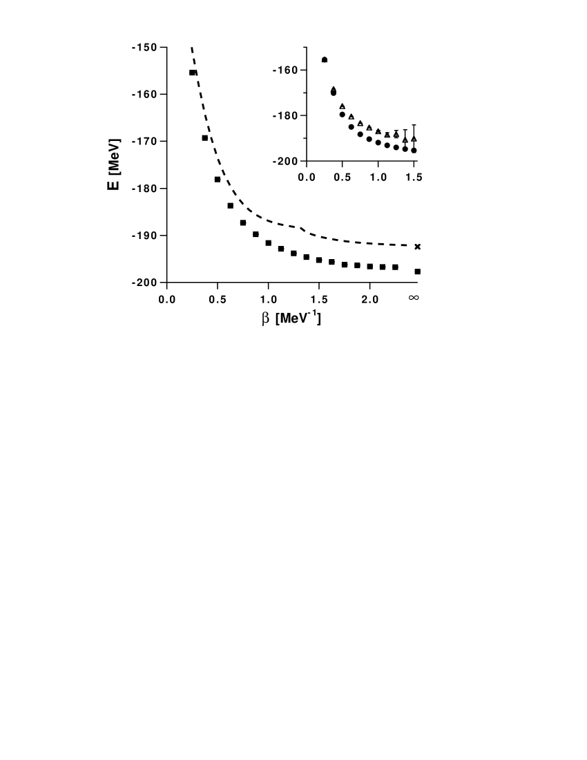
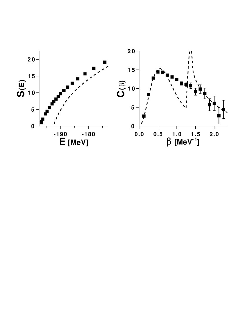
FIG. 1.: The total energy $E$ as a function of $\beta$ for ⁵⁶Fe. The SMMC values are shown by solid squares, while the HFA values by a dashed line. The inset shows the positive (circles) and negative (triangles) parity-projected SMMC energies.

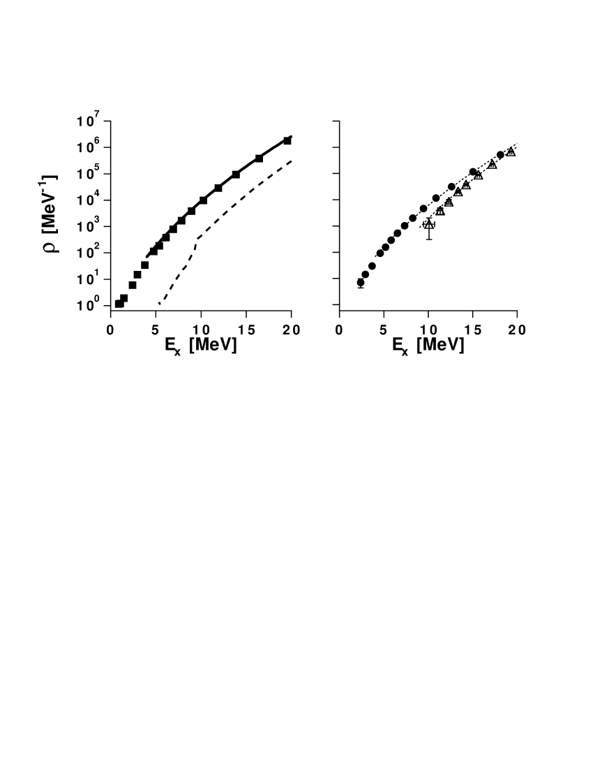
FIG. 2.: Right: the entropy as a function of energy $E$. Left: the heat capacity $C$ as a function of $\beta$. The conventions are as in Fig. 1.

FIG. 3.: Level densities of ⁵⁶Fe. Left: total level density. The SMMC level density (solid squares) is compared with the HFA level density (dashed line). The solid line is the experimental level density [20]. Right: positive- and negative-parity level densities in the SMMC. The conventions are as in the inset to Fig. 1. The dotted lines are the fit to Eq. (1) with the parameters quoted in the text.

REFERENCES

- [1] P. A. Seeger, W. A. Fowler and D. D. Clayton, Astrophys. J. Suppl. 11, 121 (1965).
- [2] A. Bohr and B. R. Mottelson, Nuclear Structure vol.1 (Benjamin, New York, 1969), p. 152, 281.
- [3] J. A. Holmes, S. E. Woosley, W. A. Fowler and B. A. Zimmerman, Atom. Data and Nucl. Data Tables 18, 305 (1976); J. J. Cowan, F.-K. Thielemann and J. W. Truran, Phys. Rep. 208, 267 (1991).
- [4] P. Quentin and H. Flocard, Ann. Rev. Nucl. Part. Sci., 28, 523 (1978); A. K. Kerman, S. Levit and T. Troudet, Ann. Phys. 148, 436 (1983).
- [5] G. H. Lang, C. W. Johnson, S. E. Koonin and W. E. Ormand, Phys. Rev. C48, 1518 (1993).
- [6] W. A. Richter, M. G. Vandermerwe, R. E. Julies and B. A. Brown, Nucl. Phys. A523, 325 (1991).
- [7] E. Caurier, A. P. Zuker, A. Poves and G. Martínez-Pinedo, Phys. Rev. C50, 225 (1994).
- [8] H. Nakada, T. Sebe and T. Otsuka, Nucl. Phys. A571, 467 (1994).
- [9] D. J. Dean, S. E. Koonin, K. Langanke, P. B. Radha and Y. Alhassid, Phys. Rev. Lett. 74, 2909 (1995).
- [10] Y. Alhassid, D. J. Dean, S. E. Koonin, G. Lang, and W. E. Ormand, Phys. Rev. Lett. 72, 613 (1994).
- [11] Y. Alhassid, G. F. Bertsch, D. J. Dean and S. E. Koonin, Phys. Rev. Lett. 77, 1444 (1996).
- [12] A. Bohr and B.R. Mottelson, Nuclear Structure vol.1 (Benjamin, New York, 1969), p.238.
- [13] T. T. S. Kuo, private communication.
- [14] G. Audi and A. H. Wapstra, Nucl. Phys. A565, 1 (1993).
- [15] D. R. Bes and R. A. Sorensen, in Advances in Nuclear Physics vol. 2, edited by M. Baranger and E. Vogt (Plenum, New York, 1969), p.129.
- [16] Y. Alhassid, S. Lenz and S. Liu, to be published.
- [17] K. Tanabe, K. Sugawara-Tanabe and H. J. Mang, Nucl. Phys. A 357, 20 (1981).
- [18] H. Junde, Nucl. Data Sheets 67, 523 (1992).
- [19] W. E. Ormand, D. J. Dean, C. W. Johnson, G. H. Lang and S. E. Koonin, Phys. Rev. C49, 1422 (1994).
- [20] S. E. Woosley, W. A. Fowler, J. A. Holmes and B. A. Zimmerman, Atom. Data and Nucl. Data Tables 22, 371 (1978).
- [21] W. Dilg, W. Schantl, H. Vonach and M. Uhl, Nucl. Phys. A217, 269 (1973).