LA-UR-97-2330

Abstract

Darwin-Foldy nuclear-size corrections in electronic atoms and nuclear radii are discussed from the nuclear-physics perspective. Interpretation of precise isotope-shift measurements is formalism dependent, and care must be exercised in interpreting these results and those obtained from relativistic electron scattering from nuclei. We strongly advocate that the entire nuclear-charge operator be used in calculating nuclear-size corrections in atoms, rather than relegating portions of it to the non-radiative recoil corrections. A preliminary examination of the intrinsic deuteron radius obtained from isotope-shift measurements suggests the presence of small meson-exchange currents (exotic binding contributions of relativistic order) in the nuclear charge operator, which contribute approximately $\textstyle{1\over 2}$%.

Recent measurements in Garching [1] and Paris [2] have greatly improved our knowledge of the isotope shift between deuterium and normal hydrogen. Due to their much increased precision[3], these measurements now rival the traditional relativistic electron scattering [4] for determining the (nuclear) sizes of these isotopes (and their differences). This new level of precision has led to a reexamination of many contributions to the level shifts [5, 6] and to the calculation of higher-order QED processes. Inevitably, a certain amount of controversy has ensued over the best way to proceed and over the proper interpretation of various mechanisms[5, 6]. Our purpose here is to discuss these topics briefly from the nuclear-physics perspective, given that these measurements have presented nuclear physics with great opportunities. Nothing that we say here is entirely new (indeed, much is very old [4, 7, 8]), but we believe that the totality casts considerable light on the interpretation and significance of these measurements.

Specifically, (1) we will (briefly) review the physics from the nuclear-physics perspective. (2) We will discuss the conventions (formalism dependence) attendant to introducing nuclear size. Although there is no right or wrong way to do this, there are consistent or inconsistent ways to proceed and there are ample opportunities for double counting. (3) We will make recommendations for avoiding such problems and discuss recent electron-scattering results[9, 10, 11] from this perspective. (4) We will make a first assessment of the d-p isotope-shift data in terms of “normal” and “exotic” components of the deuteron structure, even though the latter are not yet entirely well defined [12]. A new generation (“second generation”) of nuclear potentials [13, 14, 15] gives improved insight into deuteron structure, and this will prove useful in reducing theoretical uncertainties.

Relativistic electron scattering has traditionally been the only successful method for measuring the sizes of the lightest nuclei [4]. Muonic atoms provided significant information on heavier nuclei but until very recently electronic-atom measurements lacked the necessary precision. Nuclear physics has been investigated primarily using nonrelativistic dynamics, but the increasing precision of electron-scattering data in the late 1960’s and early 1970’s led to a reexamination [7, 8, 12] of the ways that relativity can affect a nuclear charge distribution. In order to be as specific as possible, we will first discuss various options that have arisen in discussing the simpler and better-known proton charge distribution, and then extend the discussion to light nuclei. We use natural units ($\hbar=c=1$) and the conventions and metric ($p^{2}=m^{2}$) of Ref. [16]. We also remove the proton charge, $e_{p}$, from all currents.

For historical reasons (analogy with the electron) the electromagnetic structure of the proton was introduced in terms of two form factors (i.e., Lorentz scalars): the Dirac form factor, $F_{1}(q^{2})$, and the Pauli (anomalous magnetic moment) form factor, $F_{2}(q^{2})$. The covariant current (normalized to unit charge) is given by [16]

$$J^{\lambda}=\bar{u}({\bf P}^{\prime})(\gamma^{\lambda}F_{1}(q^{2})+\frac{i\kappa_{p}}{2M}F_{2}(q^{2})\,\sigma^{\lambda\nu}q_{\nu})u({\bf P})\,,$$

where $\gamma^{\lambda}$ and $\sigma^{\lambda\nu}$ are Dirac matrices, $u({\bf P})$ and $u({\bf P}^{\prime})$ are Dirac spinors, $\kappa_{p}$ is the proton anomalous magnetic moment, $M$ is the nucleon mass, $F_{1}(0)=F_{2}(0)=1$, and $q=(P^{\prime}-P)$ is the momentum transferred (by an electron) to the final nucleon $(P^{\prime})$ from the initial one $(P)$. Because $q^{2}<0$ for scattering kinematics, it is convenient to adopt the SLAC convention, $Q^{2}\equiv-q^{2}>0$, thus avoiding inconvenient minus signs.

It was soon realized that even though $F_{2}$ primarily describes magnetic properties of the nucleon, it also contributes (in a minor way at small $Q^{2}$) to the charge distribution[17], so the Sachs[18] charge and magnetic form factors, $G_{E}$ and $G_{M}$, respectively, were introduced:

$$\hskip 108.405ptG_{E} = F_{1}(Q^{2})-\frac{\kappa_{p}Q^{2}}{4M^{2}}F_{2}(Q^{2})\,,\hskip 137.31255pt(2a)$$

$$G_{M} = F_{1}(Q^{2})+\kappa_{p}F_{2}(Q^{2})\,.\hskip 156.82576pt(2b)$$

In terms of these form factors, the (laboratory-frame) cross section for (massless) electron scattering by protons in first-Born approximation is given by the Rosenbluth formula [19, 4, 17]

$$\frac{d\sigma}{d\Omega}=\sigma_{\rm Mott}\left[A_{0}(Q^{2})+B_{0}(Q^{2})\left(\frac{1}{2}+\left(1+\frac{Q^{2}}{4M^{2}}\right)\tan^{2}(\theta/2)\right)\right]\,,$$

where $\theta$ is the electron scattering angle, $\sigma_{\rm Mott}$ is the cross section for a spinless point particle, and

$$\hskip 108.405ptA_{0}(Q^{2}) = \frac{G^{2}_{E}(Q^{2})}{1+\frac{Q^{2}}{4M^{2}}}\equiv\widetilde{G}^{2}_{E}\,,\hskip 155.38005pt(4a)$$

$$B_{0}(Q^{2}) = \frac{Q^{2}}{2M^{2}}\left[\frac{G^{2}_{M}(Q^{2})}{1+\frac{Q^{2}}{4M^{2}}}\right]\equiv\frac{Q^{2}}{2M^{2}}\widetilde{G}^{2}_{M}\,.\hskip 86.72377pt(4b)$$

Equation (3) applies to elastic electron scattering by an arbitrary nucleus, while Eq. (4) applies only to spin-$\textstyle{1\over 2}$ systems (such as the proton, ³He, or ³H ). The form factors, $\widetilde{G}_{E}$ and $\widetilde{G}_{M}$ were proposed long ago[17, 20, 4] as alternatives to $G_{E}$ and $G_{M}$, but were never popularly adopted. Equation (3) has been written so that $A_{0}$ is a form factor associated with the charge distribution, while $B_{0}$ is analogously associated with the magnetization distribution obtained from the transverse (to ${\bf\hat{q}}$) component of the (space) current. This division is most transparently performed in Coulomb gauge [7]. Often the square bracket in Eq. (3) is rearranged as [$A(Q^{2})+B(Q^{2})\tan^{2}(\theta/2)$], but then $A$ is no longer associated solely with the proton charge distribution.

One has the option of describing the proton’s structure in terms of $(F_{1},F_{2})$, $(G_{E},G_{M})$, or $(\widetilde{G}_{E},\widetilde{G}_{M})$. Only the last option correctly gauges the proton charge distribution to order $(v/c)^{2}$ (or, equivalently, $Q^{2}/M^{2}$). Factors of $\tau=Q^{2}/4M^{2}$ and $\eta=1+\tau$ are of relativistic origin and also affect the proton mean-square charge radius, defined in the Breit frame[7, 17] as $\langle r^{2}\rangle_{\rm ch}\equiv\int d^{3}x\,x^{2}\,\rho(x)$, where $J^{\lambda}=(\rho,{\bf J})$. Further defining $\langle r^{2}\rangle_{1}=-6\,F^{\prime}_{1}(0)$ and $\langle r^{2}\rangle_{E}=-6\,G^{\prime}_{E}(0)$, we obtain from Eq. (2a)

$$\langle r^{2}\rangle_{E}=\langle r^{2}\rangle_{1}+\frac{3\kappa_{p}}{2M^{2}}\,,$$

while the charge form factor obtained from Eq. (4a) produces

$$\langle r^{2}\rangle_{\rm ch}=\langle r^{2}\rangle_{E}+\langle r^{2}\rangle_{\rm DF}\,,$$

where we have defined $\langle r^{2}\rangle_{\rm ch}=-6\,\widetilde{G}^{\prime}_{E}(0)$ and

$$\langle r^{2}\rangle_{\rm DF}=\frac{3}{4M^{2}}\,.$$

The various mean-square radii, $\langle r^{2}\rangle_{1}$, $\langle r^{2}\rangle_{E}$, and $\langle r^{2}\rangle_{\rm ch}$, differ by amounts of order $\left(\frac{1}{M^{2}}\right)\sim 0.044\,{\rm fm}^{2}$, but are formally identical in the nonrelativistic (large-$M$) limit. Note that $\langle r^{2}\rangle_{E}^{1/2}$ is often called the proton radius, $r_{p}$[21].

The quantity ($3/4M^{2}$) in Eq. (5c) is the Darwin-Foldy (DF) term [16, 22] and is obtained by expanding the $1/\eta$ factor in Eq. (4a). This factor is traditionally incorporated into the kinematical factors (along with $\sigma_{\rm Mott}$) and the experimental data are then used to determine $G_{E}$ and $G_{M}$. That is, by convention, the Darwin-Foldy term is not considered part of the proton structure, even though it affects the cross section.

Nevertheless, to order ($1/M^{2}$) we can easily expand the $\lambda=0$ component of Eq. (1) to obtain the true charge density. One finds that the covariant form of $u$ (normalized to $\bar{u}u=1$) generates a frame-dependent total charge (obtained by setting $q\rightarrow 0$). The reason for this is that the wave function normalization factor $\left(\frac{1}{\sqrt{2E}}\right)$ appropriate for this convention is relegated to the phase space $\left({\rm i.e.,}\frac{d^{3}P}{(2E)(2\pi)^{3}}\right)$. If on the other hand, we incorporate that factor in $J^{\lambda}$, the phase space is $\left(\frac{d^{3}P}{(2\pi)^{3}}\right)$ and the total charge is invariant[7, 8]. The invariant form of the charge operator[16, 22] is

$$\rho\mathrel{\raise 4.0pt\hbox to9.0pt{\raise-5.0pt\hbox{$=$}\hss{$\sim$}}}\left(1-\frac{{\bf q}^{2}}{8M^{2}}\right)G_{E}+i\frac{(2G_{M}-G_{E})}{4M^{2}}\;\mbox{\boldmath$\sigma$}\;\cdot\;{\bf q}\;\times\;{\bf P},$$

where the Darwin-Foldy factor $({\bf q}^{2}/8M)$ is an explicit part of the charge operator, as is the spin-orbit interaction (expressed here in terms of the Pauli spin operator, $\sigma$). The spin-orbit interaction plays a significant role in the isotopic charge-density differences of heavier nuclei[4, 23]. Equation (6) for the charge distribution is equivalent (to ${\cal O}(1/M^{2})$) to using the form factor $\widetilde{G}_{E}$.

This daunting multiplicity of forms extends to the atomic-physics problem, as well. The Barker-Glover [24] calculation of $(Z{\alpha})^{4}$ corrections incorporated the Darwin-Foldy part of the charge density as a recoil correction of order $\left(1/M^{2}\right)$. This is most easily seen by examining the expression that serves as the baseline for defining the Lamb-shift energy[25]. Writing

$$f(n,j)\equiv\left(1+{{(Z\alpha)^{2}}\over{\left[n-j-\frac{1}{2}+\sqrt{(j+\frac{1}{2})^{2}-(Z\alpha)^{2}}\right]^{2}}}\right)^{-1/2}\,,$$

then for the state of an electron of mass $m_{e}$ specified by quantum numbers $(n,l,j)$, we have to order $(Z\alpha)^{4}/M^{2}$ for the two-body Coulomb problem

$$E_{nlj}=m_{e}+M+\mu[f(n,j)-1]-\frac{\mu^{2}}{2(m_{e}+M)}[f(n,j)-1]^{2}+\frac{(Z\alpha)^{4}\mu^{3}}{2n^{3}M^{2}}(\frac{1}{j+\frac{1}{2}}-\frac{1}{l+\frac{1}{2}})[1-\delta_{l0}],$$

where $\mu$ is the usual reduced mass. This equation can be rewritten as

$$E_{nlj}=m_{e}+M+\mu[f(n,j)-1]-\frac{\mu^{2}}{2(m_{e}+M)}[f(n,j)-1]^{2}+\frac{(Z\alpha)^{4}\mu^{3}}{2n^{3}M^{2}}(\frac{1}{j+\frac{1}{2}}-\frac{1}{l+\frac{1}{2}})+E_{\rm DF}\,,$$

where the contribution of the proton Darwin-Foldy ($\delta_{l0}$) term to the atom’s energy is

$$E_{\rm DF}=\frac{(Z\alpha)^{4}\mu^{3}}{2n^{3}M^{2}}\delta_{l0}\,.$$

The standard expression[1] for the leading-order nuclear-finite-size correction to the atom’s energy is

$$E_{\rm FS}=\frac{2(Z\alpha)^{4}\mu^{3}}{3n^{3}}\langle r^{2}\rangle_{\rm ch}\,\delta_{l0}\,,$$

and using Eq. (5c) for $\langle r^{2}\rangle_{\rm ch}$ in Eq. (7e) precisely reproduces Eq. (7d). Consequently, the DF term in an atom can be alternatively considered as part of a recoil correction of ${\cal O}(1/M^{2})$ (Eq. (7b)) or as the energy shift due to a part of the mean-square radius of the nuclear charge distribution (Eq. (7e)).

Thus, this same Darwin-Foldy term is by convention a recoil correction in atomic physics (viz., the Barker-Glover formula, Eq. (7b)) and a kinematical factor in electron scattering (viz., the Rosenbluth formula, Eq. (3)). This is perfectly allowable but somewhat confusing, since that term is part of the charge density of the proton in both cases. It is unfortunately far too late to change these conventions for the hydrogen atom. We do not recommend, however, that they be extended to other nuclei. These options were extensively discussed many years ago in the nuclear context [4] and are clearly formalism dependent (i.e., a theorist’s choice).

Equation (7b) was originally developed for the proton, but has been applied to other nuclei. For the deuteron problem Pachucki and Karshenboim[5] have argued that the DF term for a pointlike deuteron vanishes, and hence $E_{\rm DF}$ should be dropped from Eq. (7c). Khriplovich, Milstein, and Sen’kov[6] responded that only the fortuitous choice in Ref. [5] of a particular g-factor for the deuteron caused that term to vanish, and in general such a term exists. We agree with Ref.[5] that this DF term should not be included in Eq. (7c), but for different reasons. As we argue below (and as noted in Ref. [6]), the choice of inclusion or not is formalism dependent, although in general the term is not vanishing. Any such term is a part of the nuclear charge density (see the discussion below Refs. [8, 24]), and contributes a part of the mean-square radius of that density. Indeed, as we have seen, whether the proton’s DF term is a recoil correction or a nuclear-finite-size shift is also formalism dependent, although its inclusion in the standard expression (7b) is sanctioned by decades of consensus. We strongly advocate that nuclear DF terms be included as part of $\langle r^{2}\rangle_{\rm ch}$.

We examine electron scattering from the deuteron, ³H, ³He, and ⁴He in turn using Eq. (3) [7]. This is particularly relevant and topical because of the recent re-analysis of the experimental electron-deuteron scattering data by Sick and Trautmann [9]. Their derived radius, $\langle r^{2}\rangle_{\rm ch}^{1/2}=2.128(11)$ fm, is the rms radius of the complete deuteron charge density. This is typical of most nuclear calculations, which work with the charge density using the invariant convention (although there are some exceptions).

The deuteron has Z=1 and spin 1, which adds another form factor to the “charge-like” form factor, $G_{1}$, and “magnetic-like” form factor, $G_{2}$: the “quadrupole-like” form factor, $G_{3}$. Various definitions and combinations can be used, and we use the notation and definitions of Refs. [27, 28]. Because the charge-monopole (the spherical part of $\rho$) and charge quadrupole (the nonspherical part of $\rho$) contributions are incoherent (unless the deuteron spin is somehow constrained), the $A_{0}$ function of Eq. (3) becomes

$$A_{0}(Q^{2})=G^{2}_{C}+\frac{8}{9}\left[\frac{Q^{2}G_{Q}}{4M^{2}}\right]^{2},$$

where for small $Q^{2}$ the charge form factor $G_{C}$ is approximately[28]

$$G_{C}(Q^{2})\mathrel{\raise 4.0pt\hbox to9.0pt{\raise-5.0pt\hbox{$=$}\hss{$\sim$}}}G_{1}+\frac{Q^{2}}{6}Q_{d}\,,$$

while the quadrupole form factor $G_{Q}$ depends on $G_{1},G_{2}$, and $G_{3}$[28]. The static deuteron quadrupole moment is $Q_{d}=0.286\,{\rm fm}^{2}$. Equation (8b) is equivalent to corresponding forms in Refs. [5, 6, 28, 29, 30]. Defining $\langle r^{2}\rangle_{\rm ch}\,=\,-6\,G_{C}^{\prime}(0)$ and $\langle r^{2}\rangle_{1}=-6\,G^{\prime}_{1}(0)$, one finds

$$\langle r^{2}\rangle_{\rm ch}=\langle r^{2}\rangle_{1}-Q_{d}\,.$$

Note that $\langle r^{2}\rangle_{\rm ch}$ is the mean-square charge radius, and not $\langle r^{2}\rangle_{1}$; $-Q_{d}$ provides a Darwin-Foldy-type correction to $G_{1}$, and is only one part of $\langle r^{2}\rangle_{\rm ch}$. Because there are alternative form factor definitions for the deuteron, there are corresponding alternative size definitions. However, $\langle r^{2}\rangle_{\rm ch}$ is both unique and physically motivated.

The ³H and ³He cases (both having spin - $\textstyle{1\over 2}$) mirror the treatment of the proton, as in Ref. [10], where their $F_{C}(Q^{2})$ is the analogue of $G_{E}$ in Eq. (2) and $F_{C}/\eta^{1/2}$ is the complete charge form factor in the invariant representation. Reference [11], on the other hand, uses a charge operator normalized according to the covariant convention and their form factor denoted $F_{\rm ch}(Q^{2})$ differs from that of Ref. [10] by an additional factor of $\eta^{1/2}$ [$F_{\rm ch}/\eta$ is the charge form factor if one uses the invariant normalization convention]. The mean-square charge radius obtained from Ref. [10] is therefore given by ($-6\,F^{\prime}_{\rm C}(0)+3/4M^{2})$, while from Ref. [11] it is ($-6\,F^{\prime}_{\rm ch}(0)+3/2M^{2})$.

For completeness we also consider the spinless nucleus, ⁴He . The form factor and the invariant form of the charge operator for a spin-0 nucleus are the same to order $(v/c)^{2}$, and there are no DF corrections. We find[5, 6, 7, 8, 16] $B_{0}=0$,

$$\rho=\frac{(E^{\prime}+E)}{\sqrt{4E^{\prime}E}}F_{0}(Q^{2})\mathrel{\raise 4.0pt\hbox to9.0pt{\raise-5.0pt\hbox{$=$}\hss{$\sim$}}}F_{0}(Q^{2})\left(1+{\cal{O}}\left(\frac{1}{M^{4}}\right)\right)\,,$$

and $\langle r^{2}\rangle_{\rm ch}=-6\,F_{0}^{\prime}(0)$, which is another attractive property of the invariant form.

Manifest covariance, which emphasizes form factors, is the traditional way to implement special relativity, but it is not the only one. Lorentz invariance (at least to order $(v/c)^{2}$, which is the limit of our interest here) can be implemented by constructing explicit many-body representations of the Poincaré group [8, 12, 30]. In this scheme, no part of the charge density is more fundamental than any other. Rather, one works with the complete density, including “boost” effects such as the Thomas precession[31, 8]. For these reasons (based on common nuclear practice) we strongly recommend the convention that the mean-square radius of the complete nuclear charge distribution be used when computing energy shifts. This further implies that no “Darwin-Foldy” pieces of the mean-square charge radius of a nucleus should be incorporated into “recoil” corrections. If the latter is nevertheless done, it is imperative that this convention be stated explicitly.

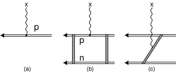
Figure 1: Deuteron and proton interactions with external electric field (curly line). The nucleons are depicted as double lines, while meson exchanges in deuterium that lead to binding or electric currents are shown as shaded double lines connecting the proton and neutron. Figure (1a) shows the proton, (1b) shows the deuteron graph that generates the “matter” radius, while (1c) illustrates meson-exchange currents. The graph showing the neutron’s finite-size contribution (identical to Fig. (1b) with the curly line attached to the neutron) is not shown.

Whatever conventions are adopted for the proton, consistency within the framework of nuclear physics (which treats nuclei as composed of nucleons) requires that the physics of the deuteron (or any heavier nucleus) incorporate Eq. (6). There will be other mechanisms allowed by the presence of additional nucleons, as well. Figure (1a) shows schematically the interaction of a single proton with an external Coulomb field. The solid dot on the double line (the proton) indicates the proton’s (finite) charge density. An identical interaction occurs in Fig. (1b) on that proton inside the deuteron, where again the solid dot indicates the full proton charge distribution including the DF term. We have indicated by shaded vertical bars on left and right the strong interactions that bind the proton and neutron together to make a deuteron. In addition to the proton interaction, the neutron has a finite size that contributes via Eq. (5b) [note that $\langle r^{2}\rangle_{\rm DF}$ vanishes for a system with no net charge]. The external field can attach to the neutron in Fig. (1b) in an identical fashion to the proton interaction. As well, the spin-orbit-interaction [7, 8] (last) term in Eq. (6) generates a small relativistic correction $\langle r^{2}\rangle_{\rm SO}$ in the bound deuteron (or any complex nucleus). Figure (1c) illustrates a generic contribution of the meson-exchange-current (denoted by MEC) type[26], where the flow of mesons that binds the deuteron generates a small contribution of relativistic order to the nuclear charge density[12].

Putting everything together, we can write for the deuteron

$$\langle r^{2}\rangle_{\rm ch}=\langle r^{2}\rangle_{m}+\langle r^{2}\rangle^{n}_{\rm ch}+\langle r^{2}\rangle^{p}_{\rm ch}+\langle r^{2}\rangle_{B}\,,$$

or, equivalently,

$$\langle r^{2}\rangle_{\rm ch}=\langle r^{2}\rangle_{\rm pt}+\langle r^{2}\rangle^{n}_{\rm ch}+\langle r^{2}\rangle^{p}_{\rm ch}\,,$$

where the part due to the binding mechanism is given by

$$\langle r^{2}\rangle_{B}=\langle r^{2}\rangle_{\rm SO}+\langle r^{2}\rangle_{\rm MEC}+\cdots\,,$$

and the “point-nucleon” radius of the deuteron is defined to be

$$\langle r^{2}\rangle_{\rm pt}=\langle r^{2}\rangle_{m}+\langle r^{2}\rangle_{B}\,.$$

The nucleon mean-square charge radii are given by Eq. (5b) [recall that $\langle r^{2}\rangle_{\rm DF}=0$ for the neutron case]. In addition, $\langle r^{2}\rangle_{m}$ is the mean-square “matter” radius, obtained directly from the square of the deuteron wave function [$\langle r^{2}\rangle_{m}\equiv\int d^{3}r|\Psi_{d}(r)|^{2}\,(r/2)^{2}$, where $r/2$ is the distance from the deuteron center-of-mass to the proton]. Equation (10) is quite general and applies to an arbitrary nucleus if a factor of $N$ (the number of neutrons) multiplies $\langle r^{2}\rangle^{n}_{\rm ch}$ and a factor of $Z$ (the number of protons) multiplies $\langle r^{2}\rangle_{\rm ch}$, $\langle r^{2}\rangle_{\rm m}$, and $\langle r^{2}\rangle^{p}_{\rm ch}$. The correction due to nuclear binding mechanisms, $\langle r^{2}\rangle_{B}$, has been written as the sum of spin-orbit contributions from the individual neutrons and protons via the last term in Eq. (6) and (potential-dependent) meson-exchange currents, plus …  . Its presence makes Eqs. (10) a definition.

In the traditional interpretation of the isotope shift[1], one calculates $\langle r^{2}\rangle_{\rm ch}-\langle r^{2}\rangle^{p}_{\rm E}$ as the measure of the finite-size difference in the isotope shift, where the first (deuteron) term incorporates a proton DF term while the second (proton) term does not. This difference then includes a term $\langle r^{2}\rangle_{\rm DF}$ from the proton in the deuteron that counterbalances a similar term implicit in the Barker-Glover recoil correction for the proton contained in Eq. (7b). This has been done consistently[1]. Thus, the proton-size effect (including the DF part) completely cancels in the $d-p$ isotope shift. This cancellation must occur on physical grounds (see Fig. (1)), irrespective of the fact that in the proton case by convention we choose to call the DF term a “recoil” correction, rather than a finite-size term.

At the level of accuracy of Ref. [3], however, this approach is no longer adequate. Each nuclear finite-size effect comes with its own reduced-mass correction (see Eq. (7e)). The proton finite-size corrections in the deuterium atom and in the hydrogen atom differ by  0.9 kHz in the 2S-1S isotope shift from this effect, although it is very tiny for the DF part alone. The finite-size correction should be calculated for each isotope with the proper reduced mass before they are subtracted.

Table 1: Calculation of the deuteron rms matter radius for a variety of potential models listed on the left. The full radius for each potential is shown in the first column of numbers, followed by the zero-range approximation for that case, and the defect mean-square radius (the difference in the squares of those columns). The final column combines the defect with the “experimental” value[41] of the zero-range approximation (1.9847(18) fm) to obtain a prediction for the full matter radius.

Potential Model	$\langle r^{2}\rangle^{1/2}\,({\rm fm})$	$\langle r^{2}\rangle_{\rm ZR}^{1/2}\,({\rm fm})$	$\Delta\langle r^{2}\rangle\,({\rm fm^{2}})$	$\langle r^{2}\rangle_{\rm m}^{1/2}\,({\rm fm})$
Second-Generation Potentials
Nijmegen (full-rel)	1.9632	1.9811	-.0705	1.9669
Nijmegen (nl-nr)	1.9659	1.9831	-.0681	1.9675
Nijmegen (nl-rel)	1.9666	1.9839	-.0683	1.9675
Nijmegen (loc-nr)	1.9671	1.9843	-.0680	1.9675
Nijmegen (loc-rel)	1.9675	1.9847	-.0680	1.9675
Reid Soft Core (93)	1.9686	1.9866	-.0709	1.9668
Argonne V18	1.9692	1.9865	-.0685	1.9674
First-Generation Potentials
Reid Soft Core (68)	1.9569	1.9683	-.0446	1.9735
Bonn (CS)	1.9687	1.9871	-.0726	1.9664
Paris	1.9714	1.9890	-.0695	1.9672
de Tourreil-Rouben-Sprung	1.9751	1.9926	-.0694	1.9672
Argonne V14	1.9816	2.0005	-.0754	1.9657
Nijmegen (78)	1.9874	2.0069	-.0780	1.9650
Super Soft Core (C)	1.9915	2.0119	-.0816	1.9641

Our final topic is a preliminary analysis of the deuteron charge radius in the non-relativistic impulse approximation[26] (i.e., the “matter” radius). The zero-range approximation[32] results from neglecting the d-state wave function and replacing the deuteron reduced s-state wave function by its asymptotic form, $A_{S}e^{-\beta r}$, where $\beta$ is the deuteron relativistic wave number and $A_{S}$ is the s-wave asymptotic normalization constant. This excellent approximation overestimates $\langle r^{2}\rangle^{1/2}$ by less than 1%. Table 1 shows a calculation of $\langle r^{2}\rangle^{1/2}$ for a wide variety of first-generation [34, 35, 36, 37, 38, 39, 40] (i.e., older) and second-generation potentials [13, 14, 15] (i.e., newer ones that fit the nucleon-nucleon scattering data from very well to exceptionally well). The full $\langle r^{2}\rangle^{1/2}$ is followed by the zero-range result for that potential. The residual, $\Delta\langle r^{2}\rangle=\langle r^{2}\rangle-\langle r^{2}\rangle_{\rm ZR}$, is next. The residual is small and for our second-generation potentials spans the range: $-0.0695(15)\;{\rm fm}^{2}$. The zero-range result using the best current values of $A_{S}$ $(0.8845(8)\;{\rm fm}^{-1/2})$ and $\beta$ [41] is $\langle r^{2}\rangle_{\rm ZR}=A^{2}_{S}/(16\beta^{3})=(1.9847(18)\;{\rm fm})^{2}$, which combines with the residual just quoted to give our best theoretical value for the root-mean-square (rms) matter radius of the deuteron:

$${}_{\rm th}\langle r^{2}\rangle^{1/2}_{m}=1.967(2)\;{\rm fm}\,.$$

Table 2: Experimental and theoretical 2S-1S deuterium-hydrogen isotope shifts in kHz. The experimental value is given on the left, followed by the theoretical value for point nuclei (with no Darwin-Foldy terms included in either non-radiative recoil contribution), the sum of nuclear polarization, nuclear Lamb shift and higher-order Coulomb finite-size contributions is next, followed on the right by the leading-order nuclear finite-size contribution (including all nuclear Darwin-Foldy terms) adjusted to produce agreement with the experimental isotope shift.

experimental	point nuclei	misc. nuclear	nuclear size
670 994 334(2)	670 999 503.2	19.2	-5188.4

This result is our baseline, from which deviations signal “exotic” components of the deuteron charge density. We can make our own estimate of this deviation by using the current experimental value[3] of the 1S-2S isotope shift: 670 994 334(2) kHz. We also use an updated version of the theoretical analysis presented in Ref. [1], which is displayed in Table 2. We use the improved $\frac{m_{p}}{m_{e}}$ ratio of Ref. [42] (1836.1526665(40)) and the $\frac{m_{d}}{m_{p}}$ ratio of Ref. [43] (1.9990075009(8)). We also use the improved deuteron polarizability of Ref. [44]; the proton polarizability of Ref. [45] cancels in the isotopic difference. Higher-order $(Z\alpha)^{5}$ and $(Z\alpha)^{6}$ Coulomb finite-size corrections are obtained from Ref. [46]. The neutron mean-square charge radius is taken from Ref. [47]: $\mbox{$-$}0.1140(26)~{}{\rm fm}^{2}$. All other constants are taken from Ref. [48]. Using the deuteron mean-square charge radii defined by Eq. (10), we obtain the experimental value of the deuteron point-nucleon radius

$${}_{\rm exp}\langle r^{2}\rangle_{\rm pt}^{1/2}=1.9753(11)\;{\rm fm}\,,$$

and

$${}_{\rm exp}\langle r^{2}\rangle_{\rm pt}^{1/2}-\,{{}_{\rm th}\langle r^{2}\rangle_{\rm m}^{1/2}}=0.008(2)\;{\rm fm}\,,$$

where the error in Eq. (12) is obtained by compounding a 1.5 kHz $\frac{m_{p}}{m_{e}}$ uncertainty, the 2 kHz experimental uncertainty, an estimated 4 kHz uncertainty in QED calculations[1], and an (equivalent) 3.5 kHz uncertainty from the neutron charge radius. These results are shown in Table 3. On the scale of these uncertainties the DF terms discussed earlier are very large for the 2S-1S transition, approximately 45 kHz/$A^{2}$ ($A$ is the nucleon number), where roughly 5 kHz changes $\langle r^{2}\rangle^{1/2}_{\rm ch}$ by 0.001 fm.

Table 3: Experimental and theoretical deuteron radii. The deuteron matter radius corresponding to second-generation nuclear potentials renormalized to the experimental zero-range approximation and the experimental point-nucleon charge radius of the deuteron are shown in the first two columns, followed by the difference of experimental and theoretical results. Relativistic corrections to the mean-square charge radius from the electromagnetic spin-orbit interaction and from MEC (assuming minimal nonlocality) are listed in the next two columns. The final theoretical estimate of the charge radius for pointlike nucleons is listed in the sixth column. No uncertainty is given in the final estimate because of consistency problems between the MEC and the nuclear potentials.

${}_{\rm th}\langle r^{2}\rangle_{\rm m}^{1/2}\,({\rm fm})$	${}_{\rm exp}\langle r^{2}\rangle_{\rm pt}^{1/2}\,({\rm fm})$	Diff. (fm)	$\langle r^{2}\rangle_{\rm SO}\,({\rm fm^{2}})$	$\langle r^{2}\rangle_{\rm MEC}\,({\rm fm^{2}})$	${}_{\rm th}\langle r^{2}\rangle_{\rm pt}^{1/2}\,({\rm fm})$
1.967(2)	1.9753(11)	0.008(2)	-0.0014	0.0159	1.971

The atomic results above can be contrasted with the less precise determination of $\langle r^{2}\rangle^{1/2}_{\rm pt}$ using Eqs. (10) and the electron scattering results of Refs. [9, 21]:

$${}_{\rm exp}\langle r^{2}\rangle^{1/2}_{\rm pt}=1.966(13)\;{\rm fm}\,,$$

from which we obtain

$${}_{\rm exp}\langle r^{2}\rangle_{\rm pt}^{1/2}-\,{{}_{\rm th}\langle r^{2}\rangle_{\rm m}^{1/2}}=-0.001(13)\;{\rm fm}\,.$$

At this level of precision, the result (15) is null. Equations (10b) and (12) lead to a full deuteron charge radius from the isotope shift of 2.136(5) fm, which is consistent with the value of 2.128(11) fm from Ref. [9].

Although the result (13) is effectively nonzero, there is one caveat about its significance. The matter radius derived earlier is not entirely well defined. It was shown long ago [12] that to order $(v/c)^{2}$ there are 2 unitary equivalences that arise naturally in treating relativistic corrections; these are the (pion) chiral-rotation equivalence specified by a parameter, $\mu$, and the quasi-potential equivalence (similar to electromagnetic gauge-dependence) specified by a parameter, $\nu$. These parameters modify the nuclear potential through nonlocal terms, and also modify the nuclear charge operator through meson-exchange currents. Because none of the representations corresponds precisely to a nonrelativistic (i.e., momentum-independent) potential, no specification of $\mu$ and $\nu$ is possible without performing a consistent relativistic calculation (at least to order $(v/c)^{2}$). Since a unitary transformation cannot change observables (and hence the zero-range approximation is unchanged), only the defect wave function and the defect mean-square radius $(\langle r^{2}\rangle_{m}-\langle r^{2}\rangle_{\rm ZR})$ can be changed and both will therefore depend on $\mu$ and $\nu$, as will $\langle r^{2}\rangle_{\rm MEC}$. Both ($\langle r^{2}\rangle_{\rm m}+\langle r^{2}\rangle_{\rm MEC}$) and $\langle r^{2}\rangle_{\rm ch}$ do not. We can stipulate conditions on the potential that will restrict the parameters $\mu$ and $\nu$. One condition is “minimal nonlocality”, which requires the nuclear tensor force to be as local as possible and the entire force to be energy independent. This is equivalent to $\mu=0$ and $\nu=1/2$[12], and bears a rough correspondence to Coulomb gauge in atomic physics. Such a representation is probably the closest to (but not quite the same as) using the local potentials that are the norm in nuclear physics. This representation for the MEC charge operator is well known [12] and produces

$$\langle r^{2}\rangle_{\rm MEC}\left|{}_{\stackrel{{\scriptstyle\mu=0}}{{\nu=1/2}}}\mathrel{\raise 4.0pt\hbox to9.0pt{\raise-5.0pt\hbox{$=$}\hss{$\sim$}}}0.0159\,{\rm fm}^{2}\,,\right.$$

and together with

$$\langle r^{2}\rangle_{\rm SO}\mathrel{\raise 4.0pt\hbox to9.0pt{\raise-5.0pt\hbox{$=$}\hss{$\sim$}}}-0.0014\,{\rm fm}^{2}\,,$$

one finds the full radius

$${}_{\rm th}\langle r^{2}\rangle^{1/2}_{\rm pt}=1.971\,{\rm fm}\,,$$

which makes up approximately half the difference between the experimental value and the baseline estimate predicated on nonrelativistic second-generation potentials: $(\langle r^{2}\rangle^{1/2}_{\rm pt}-\langle r^{2}\rangle^{1/2}_{m})$ given in Table 3. Hopefully, the remaining .004 fm comes from the difference between a true relativistic treatment of the deuteron and our nonrelativistic one that we have supplemented with (somewhat) ad hoc corrections. Our results for $\langle r^{2}\rangle_{\rm B}$ are similar to those of Ref. [49].

In summary, we have reviewed the various ways that nuclear sizes are incorporated into electron scattering and atomic calculations. We strongly recommend the convention that complete nuclear charge radii be used in calculating atomic energy shifts, rather than radii based on arbitrary form factor definitions. A “baseline” value of the deuteron rms radius was calculated using nonrelativistic second-generation potentials to correct the (excellent) zero-range approximation. A value of the deuteron rms radius extracted from the d-p isotope shift is .008(2) fm larger than this baseline value, some of which is almost certainly due to meson-exchange currents. A complete resolution of the problem caused by this difference awaits a relativistic treatment of the deuteron dynamics[50] that is of “second-generation” quality, because we are dealing with very small size differences.

Acknowledgements

The work of J. L. F. was performed under the auspices of the United States Department of Energy. D. W. L. S. is grateful to NSERC Canada for continued support under Research Grant No. SAP00-3198. The work of J. M. is supported under Grant No. PB94-0900 of DGES, Spain. We would like to thank T. W. Hänsch for providing information about his experiments, I. Khriplovich for a useful discussion about g-factors, and K. Pachucki for useful comments on an early version of this manuscript.

References

- [1] K. Pachucki, D. Leibfried, M. Weitz, A. Huber, W. Konig, and T. W. Hänsch, J. Phys. B29, 177 (1996) contains an excellent summary of recent experimental and theoretical progress.
- [2] B. de Beauvoir, F. Nez, L. Julien, B. Cagnac, F. Biraben, D. Touahri, L. Hilico, O. Acef, A. Clairon, and J. J. Zondy, Phys. Rev. Lett. 78, 440 (1997).
- [3] T. W. Hänsch, Invited talk at 12th Interdisciplinary Laser Science Conference, Rochester, N. Y., Oct. 20, 1996; T. W. Hänsch, Invited talk at APS Spring Meeting, Washington DC, April 20, 1997; T. W. Hänsch (private communication).
- [4] J. L. Friar and J. W. Negele, Adv. in Nucl. Phys. 8, 219 (1975). This work reviews elastic electron-nucleus scattering and muonic atoms, and includes an extensive discussion of Darwin-Foldy terms.
- [5] K. Pachucki and S. G. Karshenboim, J. Phys. B 28, L221 (1995).
- [6] I. B. Khriplovich, A. I. Milstein, and R. A. Sen’kov, Phys. Lett. A 221, 370 (1996).
- [7] J. L. Friar, Ann. Phys. (N. Y. ) 81, 332 (1973).
- [8] J. L. Friar, Nucl. Phys. A264, 455 (1976). See also J. L. Friar, B. F. Gibson, and G. L. Payne, Phys. Rev. C 30, 441 (1984). These references established the form of the nuclear charge and current operators to order . Neglecting terms of third and higher order in momenta and terms whose expectation value vanishes, one finds: and , where the nuclear velocity is is the nuclear magnetic moment, is the nuclear spin, is the nuclear quadrupole tensor (if allowed), and is the mean-square radius of the nuclear charge distribution. The nuclear spin, magnetic, and quadrupole terms contribute in leading order solely to the hyperfine interactions. Only the nuclear convection current (via recoil corrections) and nuclear finite size remain to supplement the charge. Note also that the nuclear velocity-dependent terms in vanish in both the lab frame () and the Breit frame ().
- [9] I. Sick and D. Trautmann, Phys. Lett. B 375, 16 (1996). This work incorporated Coulomb distortion into the cross section analysis for the first time. These distortions increased the charge radius over previously obtained values[32, 33].
- [10] D. Beck et al., Phys. Rev. Lett. 59, 1537 (1987).
- [11] A. Amroun et al., Nucl. Phys. A579, 596 (1994).
- [12] S. A. Coon and J. L. Friar, Phys. Rev. C 34, 1060 (1986); J. L. Friar, Phys. Rev. C 22, 796 (1980). The Appendix of the first reference lists the properties of various () representations. The choice , which minimizes the MEC corrections to the electric-dipole operator as well as simplifying the nuclear potential, was first discussed here.
- [13] J. L. Friar, G. L. Payne, V. G. J. Stoks, and J. J. de Swart, Phys. Lett. B 311, 4 (1993).
- [14] V. G. J. Stoks, R. A. M. Klomp, C. P. F. Terheggen, and J. J. de Swart, Phys. Rev. C 49, 2950 (1994). See also, V. G. J. Stoks, R. A. M. Klomp, M. C. M. Rentmeester, and J. J. de Swart, Phys. Rev. C 48, 792 (1993).
- [15] R. B. Wiringa, V. G. J. Stoks, and R. Schiavilla, Phys. Rev. C 51, 38 (1995).
- [16] J. D. Bjorken and S. D. Drell, Relativistic Quantum Mechanics, (McGraw-Hill, New York, 1964). We use the metric and conventions of this reference.
- [17] D. R. Yennie, M. M. Levy, and D. G. Ravenhall, Rev. Mod. Phys. 29, 144 (1957) reviews the early history of this topic. Their Eq. (2.11) is our Eq. (5), while their Eq. (A-23) is our Eq. (4a).
- [18] R. G. Sachs, Phys. Rev. 126, 2256 (1962).
- [19] M. N. Rosenbluth, Phys. Rev. 79, 615 (1950).
- [20] M. Gourdin, Nuovo Cimento 36, 1409 (1965).
- [21] G. G. Simon, C. Schmidt, F. Borkowski, V. H. Walter, Nucl. Phys. A333, 381 (1980). A more recent evaluation of the data can be found in, P. Mergell, Ulf-G. Meißner and D. Drechsel, Nucl. Phys. A596, 367 (1996).
- [22] L. L. Foldy and S. A. Wouthuysen, Phys. Rev. 78, 29 (1950).
- [23] W. Bertozzi, J. L. Friar, J. Heisenberg and J. W. Negele, Phys. Lett. 41B, 408 (1972).
- [24] W. A. Barker and F. N. Glover, Phys. Rev. 99, 317 (1955). Neglecting hyperfine-interaction terms, the nuclear convection current is the only frame-dependent nuclear interaction that contributes to recoil corrections (through terms quadratic in momenta)[see the discussion below Ref. [8]]. Incorporating this interaction plus the nuclear kinetic energy into the electron dynamics generates Eq. (7c) without , which is a part of the nuclear charge-radius finite-size correction.
- [25] J. R. Sapirstein and D. R. Yennie, in Quantum Electrodynamics, ed. by T. Kinoshita, (World Scientific, Singapore, 1990), p. 560. This comprehensive review defined the state of the art at the time of its publication.
- [26] J. L. Friar, Czech. J. Phys. 43, 259 (1993); H. Arenhövel, Czech. J. Phys. 43, 207 (1993) are introductory articles treating meson-exchange currents. Neglecting such currents and other binding effects is denoted the “impulse approximation”.
- [27] F. Gross, in Modern Topics in Electron Scattering, ed. by B. Frois and I. Sick (World Scientific, Singapore, 1991), p. 219. This lovely review thoroughly and clearly discusses relativistic effects in nuclear electromagnetic interactions.
- [28] R. G. Arnold, C. E. Carlson, and F. Gross, Phys. Rev. C 21, 1426 (1980). They define , where and ( and are the initial and final deuteron polarization (momentum) four-vectors and is the deuteron mass. The corresponding charge, quadrupole, and magnetic form factors are given by , , and . The deuteron form factors used in other references can be written as linear combinations of the , , introduced here, or are identical but use different notation.
- [29] M. J. Zuilhof and J. A. Tjon, Phys. Rev. C 22, 2369 (1980).
- [30] F. Coester and A. Ostebee, Phys. Rev. C 11, 1836 (1975); P. L. Chung, F. Coester, B. D. Keister, and W. N. Polyzou, Phys. Rev. C 37, 2000 (1988). These references define in Eq. (3) directly in terms of the spin-averaged square of the charge density in the Breit frame.
- [31] S. J. Brodsky and J. R. Primack, Ann. Phys. (N. Y. ) 52, 315 (1969); R. A. Krajcik and L. L. Foldy, Phys. Rev. D 10 1777 (1974); J. L. Friar, Phys. Rev. C 16, 1504 (1977). These references discuss the electromagnetic spin-orbit interaction and its relevance to Compton low-energy theorems and sum rules, as well as g-factors and anomalous magnetic moments, for such complex systems as nuclei.
- [32] S. Klarsfeld, J. Martorell, J. A. Oteo, M. Nishimura, and D. W. L. Sprung, Nucl. Phys. A456, 373 (1986); R. K. Bhaduri, W. Leidemann, G. Orlandini, and E. L. Tomusiak, Phys. Rev. C 42, 1867 (1990); D. W. L. Sprung, Hua Wu and J. Martorell, Phys. Rev. C 42, 863 (1990). These references determine the dependence of the deuteron-radius defect function on various nuclear parameters. Note that our is called in these references.
- [33] C. W. Wong, Int. J. Mod. Phys. E 3, 821 (1994).
- [34] R. V. Reid, Ann. Phys. (N. Y. ) 50, 411 (1968).
- [35] R. Machleidt, K. Holinde, and C. Elster, Phys. Rep. 149, 1 (1987).
- [36] M. Lacombe, B. Loiseau, J. M. Richard, R. Vinh Mau, J. Côté, P. Pirès, and R. de Tourreil, Phys. Rev. C 21, 861 (1980).
- [37] R. de Tourreil, B. Rouben, and D. W. L. Sprung, Nucl. Phys. A242, 445 (1975).
- [38] R. B. Wiringa, R. A. Smith, and T. A. Ainsworth, Phys. Rev. C 29, 1207 (1984).
- [39] M. M. Nagels, T. A. Rijken, and J. J. de Swart, Phys. Rev. D 17, 768 (1978).
- [40] R. de Tourreil and D. W. L. Sprung, Nucl. Phys. A201, 193 (1973).
- [41] J. J. de Swart, C. P. F. Terheggen, V. G. J. Stoks, Nijmegen preprint THEF-NYM-95.11, nucl-th/9509032, Proc. of Third Int. Symposium ”Dubna Deuteron 95”, Dubna, Russia, July ’95; J. J. de Swart, R. A. M. Klomp, M. C. M. Rentmeester, Th. A. Rijken, Few-Body Systems Suppl. 99, (1995) and THEF-NYM-95.08.
- [42] D. L. Farnham, R. S. Van Dyck, Jr., and P. B. Schwinberg, Phys. Rev. Lett. 75, 3598 (1995).
- [43] G. Audi and A. H. Wapstra, Nucl. Phys. A595, 409 (1995).
- [44] J. L. Friar and G. L. Payne, nucl-th/9704032; Phys. Rev. C (in press).
- [45] I. B. Khriplovich, and R. A. Sen’kov, nucl-th/9704043. Just as the proton size cancels in the d-p isotope shift, the proton polarizability also occurs in the deuteron, and hence will cancel in the isotope shift. The neutron polarizability in the deuteron has not been included in our calculations.
- [46] J. L. Friar and G. L. Payne, nucl-th/9705036; Phys. Rev. C (submitted).
- [47] S. Kopecky, P. Riehs, J. A. Harvey, and N. W. Hill, Phys. Rev. Lett. 74, 2427 (1995). We used the compiled value at the bottom on Table I.
- [48] E. R. Cohen and B. N. Taylor, Rev. Mod. Phys. 59, 1121 (1987). All constants are taken from this work unless otherwise noted.
- [49] A. J. Buchmann, H. Henning, and P. U. Sauer, Few-Body Systems 21, 149 (1996).
- [50] L. P. Kaptari et al., Phys. Rev. C 54, 986 (1996).