TPR-97-12

Fine-Tuning Two-Particle Interferometry
I: Effects from Temperature Gradients in the Source

Boris Tomášik and Ulrich Heinz

Institut für Theoretische Physik, Universität Regensburg,
D-93040 Regensburg, Germany

September 24, 1997

A comprehensive model study of Bose-Einstein correlation radii in heavy ion collisions is presented. The starting point is a longitudinally and transversally expanding fireball, represented at freeze-out by an azimuthally symmetric emission function. The freeze-out temperature is allowed to feature transverse and temporal gradients. Their effects on the correlation radii are studied. In particular, we evaluate numerically their dependence on the transverse mass of the particle pairs and check a recent suggestion, based on analytical approximations, that for certain reasonable source parameters all three correlation radii satisfy simultaneously a $1/\sqrt{M_{\perp}}$ scaling.

1 Introduction

Recently, two-particle intensity interferometry, exploiting the effects of Bose-Einstein (BE) symmetrization on the two-particle momentum spectra, has been developed into a powerful tool for measuring not only the space-time dimensions of the particle emitting object, but also its dynamical state at particle freeze-out. Modern Bose-Einstein interferometry thus goes far beyond the original work by Hanbury Brown and Twiss, who introduced and successfully demonstrated photon intensity interferometry for static sources in astrophysics [1], and the pioneering paper by Goldhaber, Goldhaber, Lee, and Pais [2] who first exploited similar ideas in particle physics. Good reviews of the basic theoretical and experimental techniques can be found in [3, 4, 5, 6, 7] while the more recent theoretical developments are summarized in a series of lectures published in [8].

Collective dynamics of the source leads to a characteristic dependence of the two-particle correlation function on the total momentum of the particle pair. The width of the correlator as a function of the relative momentum of the two particles measures the size of the “regions of homogeneity” [9] inside the source across which the momentum distribution changes sufficiently little to guarantee measurable rates for pairs with similar momenta of the two particles. For rapidly expanding sources widely separated points do not emit particles of similar momenta; the homogeneity regions seen by BE correlation function thus form only a fraction of the whole source. Moreover, the momentum of a particle defines the homogeneity region from which it is coming; we will call the homogeneity region which contributes to the emission of particles with a given momentum the “effective source” for such particles.

The size parameters of the “effective source” (which are measured by the correlator and which we will thus call “correlation radii” or simply “HBT radii”) are related to the magnitude of the velocity gradients in the source, multiplied with a thermal smearing factor $\sqrt{T/M_{\perp}}$ originating from the local momentum distribution [10, 11, 12]. They are thus affected by both the expansion velocity profile of the source and by variations of the width (“temperature”) of the local momentum distributions across the source [11, 13, 14, 15, 16]. Another physical mechanism which can, even in the absence of flow and temperature gradients, lead to dramatic differences between the “effective source” of particles with a fixed momentum $K$ and the momentum-integrated distribution of source points in space-time is strong reabsorption or rescattering of the particles in the interior of the source; this leads to a surface-dominated distribution of last interaction points with a strong preference for outward-directed momenta. Such “opaque sources” and their effects on the correlation radii have recently been discussed in [17, 18] on a semianalytic level using simple models. Our investigations on this subject will be published in the next paper [19].

While the basic relations between such source features as mentioned above and the properties of the measurable two-particle correlation functions appear to be qualitatively understood, this is not sufficient for a quantitative interpretation of two-particle correlation data and a complete reconstruction of the source from the measurements. Quantitative numerical investigations, including comprehensive parameter studies, so far exist mostly for transparent expanding sources with constant freeze-out temperature [12, 20, 21, 22], while for sources with temperature gradients some numerical checks of the approximate analytical approximations developed in [13, 14, 15] have been performed in [23, 24]. In [23] the validity range of the analytical formulae given in [14] was determined. A comparison with experimental data from 200 $A$ GeV/$c$ S+Pb collisions [25] in [24] revealed, however, that the required source parameters lie outside this range of validity. A quantitative comparison with data thus requires numerical studies.

In this paper we present a numerical parameter study of the influence of flow and temperature gradients on the correlation radii. One goal of this investigation is to settle a question which was left open in [23, 24]: based on a series of approximations, the authors of [14] had found a common $1/\sqrt{M_{\perp}}$ scaling law for all three HBT radii $R_{s}$, $R_{o}$, $R_{l}$ in a Cartesian parametrisation of the correlator. This was desirable in view of the S+Pb data of [25] where agreement with such a common scaling law was reported (although supported only by three data points in each Cartesian direction). The data of [26, 27, 28, 29, 30, 31] from S+S, S+Ag, S+Au, and Pb+Pb collisions, on the other hand, all show a much stronger $M_{\perp}$-dependence of the longitudinal HBT radii compared to the transverse ones. This is in qualitative agreement with the theoretical studies in [12, 20, 21] which, for sources with constant temperature and boost-invariant longitudinal, but weaker transverse expansion, show a weaker $M_{\perp}$-dependence for $R_{s}$ than for $R_{l}$. In [12, 21] it was argued that, if one fits the $M_{\perp}$-dependence of the HBT radii with a negative power law, $R_{i}(M_{\perp})\sim M_{\perp}^{-\alpha_{i}}$ [27, 28, 31], the power $\alpha_{i}$ itself should be proportional to the rate of expansion in direction $i$; this feature cannot be obtained within the simple saddle point approximation used in [10, 11, 13, 14, 16, 32]. We show here that, within the phenomenologically allowed parameter range, this remains true even in the presence of temperature gradients.

In contrast to the work of [23, 24] we also compute the HBT radii in the Yano-Koonin-Podgoretskiĭ (YKP) parametrisation of the correlation function [33, 34, 32] which have a more straightforward and simpler interpretation in space-time [32, 21] than the HBT parameters from the Cartesian (Pratt-Bertsch-Chapman) parametrisation [10, 11]. As far as we know, the effects of temperature gradients on the YKP parameters have not been studied before.

We want to stress that resonance decays are not addressed in this paper. It is known that they can strongly affect the correlation function [35, 36, 37, 38, 39, 40] in which case a Gaussian parametrisation as employed here becomes questionable [40, 41, 42]. Thus, while our calculations refer both to pion and kaon correlations, only the kaon results and those for high-$K_{\perp}$ pions (where resonance decays can be neglected) can be directly related to data. For low-$K_{\perp}$ pion pairs our results show the features of the contribution from directly emitted pions to the correlator.

2 Formalism

For chaotic sources the two-particle correlation function is in very good approximation given by the formula [43, 44, 45]

$$C(q,K)\simeq 1+\frac{{\left|\int d^{4}x\,S(x,K)\,e^{iq.x}\right|}^{2}}{{\left|\int d^{4}x\,S(x,K)\,\right|}^{2}}\,.$$ (1)

Here $S(x,K)$ is the emission function (single-particle Wigner phase-space density) of the source [43, 44, 45], and $K=\frac{1}{2}(p_{1}+p_{2})$ (with $p_{1,2}$ on-shell) is the average pair momentum while $q=p_{1}-p_{2}$ denotes the momentum difference between the two particles.

One usually parameterizes the correlation function by a Gaussian in $q$ [20, 21]. Since $q$ satisfies the on-shell constraint $q\cdot K=0$, only three of its four components are independent. This leaves room for various (mathematically equivalent) Gaussian parametrisations, using different sets of independent $q$-components. Here we will consider only azimuthally symmetric sources and evaluate the parameters (HBT radii) of the Cartesian and of the Yano-Koonin-Podgoretskiĭ (YKP) parametrisations, in the commonly used coordinate system where the $z$ axis defines the beam direction and ${\bf K}$ lies in the $x-z$ plane. The $x$ axis is customarily labeled as $o$ (for outward), $y$ as $s$ (for sideward), and $z$ as $l$ (for longitudinal).

The Cartesian parametrisation of the correlator employs the three spatial components of $q$ in the form [10, 11]

$$C({\bf q},{\bf K})=1+\exp\left[-R_{s}^{2}({\bf K})q_{s}^{2}-R_{o}^{2}({\bf K})q_{o}^{2}-R_{l}^{2}({\bf K})q_{l}^{2}-2R_{ol}^{2}({\bf K})q_{o}q_{l}\right]\,.$$ (2)

The four ${\bf K}$-dependent parameters (HBT radii) are then given by linear combinations of the space-time variances of the effective source of particles with momentum $K$ [10, 11, 46]:

$$R_{s}^{2}({\bf K}) = \langle\tilde{y}^{2}\rangle\,,$$ (3)

$$R_{o}^{2}({\bf K}) = \langle(\tilde{x}-\beta_{\perp}\tilde{t})^{2}\rangle\,,$$ (4)

$$R_{l}^{2}({\bf K}) = \langle(\tilde{z}-\beta_{l}\tilde{t})^{2}\rangle\,,$$ (5)

$$R_{ol}^{2}({\bf K}) = \langle(\tilde{x}-\beta_{\perp}\tilde{t})(\tilde{z}-\beta_{l}\tilde{t})\rangle\,.$$ (6)

The angular brackets denote space-time averages taken with the emission function $S(x,K)$ of the effective source at momentum $K$, and coordinates with a tilde are measured relative to the center of the effective source: $\tilde{x}_{\mu}=x_{\mu}-\bar{x}_{\mu}\,,\bar{x}_{\mu}=\langle x_{\mu}\rangle$ [20].

In the LCMS (Longitudinally CoMoving System [47]), where $\beta_{l}=K_{l}=0$, $R_{l}^{2}$ and $R_{ol}^{2}$ simplify to

$$R_{l}^{2} = \langle{\tilde{z}}^{2}\rangle\,,$$ (7)

$$R_{ol}^{2} = \langle(\tilde{x}-\beta_{\perp}\tilde{t})\,\tilde{z}\rangle\,.$$ (8)

For further discussions of these expressions see [10, 11].

The YKP parametrisation employs the components $q^{0}$, $q_{\perp}=\sqrt{q_{o}^{2}+q_{s}^{2}}$, and $q_{l}$ in the form [32, 20, 21]

$$C({\bf q},{\bf K})=1+\exp\left[-R_{\perp}^{2}({\bf K})\,q_{\perp}^{2}-R_{\parallel}^{2}({\bf K})\left(q_{l}^{2}{-}(q^{0})^{2}\right)-\left(R_{0}^{2}({\bf K}){+}R_{\parallel}^{2}({\bf K})\right)\left(q{\cdot}U({\bf K})\right)^{2}\right].$$ (9)

The YKP radii $R_{\perp}$, $R_{\parallel}$, and $R_{0}$ are invariant under longitudinal boosts of the measurement frame; they measure (in some approximation) the transverse, longitudinal, and temporal extension of the effective source in its longitudinal rest frame (called Yano-Koonin (YK) frame) [32, 20, 21]. This frame moves with the YK velocity $v({\bf K})$, defined by the fourth fit parameter $U({\bf K})$ via

$$U({\bf K})=\gamma({\bf K})\,(1,0,0,v({\bf K})),\qquad\gamma({\bf K})=\frac{1}{\sqrt{1-v^{2}({\bf K})}}\,.$$ (10)

The YKP parameters can be calculated from the emission function through relations similar to (3)-(6): Defining [20, 21]

$$A = \left\langle\left(\tilde{t}-{\tilde{\xi}\over\beta_{\perp}}\right)^{2}\right\rangle\,,$$ (11)

$$B = \left\langle\left(\tilde{z}-{\beta_{l}\over\beta_{\perp}}\tilde{\xi}\right)^{2}\right\rangle\,,$$ (12)

$$C = \left\langle\left(\tilde{t}-{\tilde{\xi}\over\beta_{\perp}}\right)\left(\tilde{z}-{\beta_{l}\over\beta_{\perp}}\tilde{\xi}\right)\right\rangle\,,$$ (13)

with $\tilde{\xi}\equiv\tilde{x}+i\tilde{y}$ such that $\langle\tilde{\xi}^{2}\rangle=\langle\tilde{x}^{2}-\tilde{y}^{2}\rangle$, they are given by

$$v = {A+B\over 2C}\left(1-\sqrt{1-\left({2C\over A+B}\right)^{2}}\right)\,,$$ (14)

$$R_{\parallel}^{2} = B-v\,C\,,$$ (15)

$$R_{0}^{2} = A-v\,C\,,$$ (16)

$$R_{\perp}^{2} = {\langle{\tilde{y}^{2}}\rangle}\,.$$ (17)

Note that the Yano-Koonin velocity $v$, and thus $R_{\parallel}$ and $R_{0}$, are well-defined only for effective sources with $(A+B)^{2}-4C^{2}\geq 0$. It will be shown in [19] that this condition can be violated in particular for opaque sources. In the limit $C\to 0$ the YK velocity $v$ vanishes such that this condition defines the YK frame. In this frame $R_{\parallel}^{2}=B$ and $R_{0}^{2}=A$.

As a side remark, we would like to note that the quantities $A,B,C$ from Eqs. (11)-(13) are identical with the radius parameters introduced in [22, 40, 42], where a different Cartesian parametrisation based on the same $q$-components as in the YKP case was used:

$$C({\bf q},{\bf K})=1+\exp[-R_{\perp}^{2}({\bf K})q_{\perp}^{2}-R_{z}^{2}({\bf K})q_{l}^{2}-R_{t}^{2}({\bf K})(q^{0})^{2}-2\,R_{zt}^{2}({\bf K})q_{l}q^{0}]\,.$$ (18)

One easily shows

$$R^{2}_{t}=A\,,\quad R^{2}_{z}=B\,,\quad R^{2}_{zt}=-C\,.$$ (19)

Clearly, these parameters are not boost-invariant and thus don’t lead directly to a simple space-time interpretation of the correlator. Their usefulness is rather of technical nature in the actual data fitting procedure [22, 40, 42] and, of course, the YKP parameters can be reconstructed from them via Eqs. (14)-(16).

Our calculations in the following sections of the correlation radii will be based on the expressions (3)-(8) and (11)-(17).

3 Hydrodynamic parametrisation of the source

For our studies we use slightly modified (see Appendix A) model of [14]:

$$S(x,K)\,d^{4}x = {M_{\perp}\cosh(\eta-Y)\over(2\pi)^{3}}\;\exp\left[-{K\cdot u(x)\over T(x)}\right]\;\exp\left[-{r^{2}\over 2R^{2}}-{{(\eta-\eta_{0})}^{2}\over 2(\Delta\eta)^{2}}\right]$$ (20)

$$\times\frac{\tau\,d\tau}{\sqrt{2\pi(\Delta\tau)^{2}}}\;\exp\left[-{(\tau-\tau_{0})^{2}\over 2(\Delta\tau)^{2}}\right]\,d\eta\,r\,dr\,d\phi.$$

This “emission function” parametrizes the distribution of points of last interaction in the source. The parametrisation (20) is motivated by hydrodynamical models with approximately boost-invariant longitudinal dynamics. It uses thermodynamic and hydrodynamic parameters and appropriate coordinates; for a detailed discussion see, e.g., [8]. In the calculations we use the on-shell approximation $K_{0}\approx E_{K}=\sqrt{m^{2}+{\bf K}^{2}}$ as discussed in [11].

The velocity field $u(x)$ determines the dynamics of the source at freeze-out. We parametrize it by [12]

$$u^{\mu}(x)=\left(\cosh\eta\cosh\eta_{t}(r),\,\cos\phi\,\sinh\eta_{t}(r),\,\sin\phi\,\sinh\eta_{t}(r),\,\sinh\eta\cosh\eta_{t}(r)\right),$$ (21)

thereby implementing a boost-invariant longitudinal flow profile $v_{L}=z/t$, with a linear radial profile of strength $\eta_{f}$ for the transverse flow rapidity:

$$\eta_{t}(r)=\eta_{f}{r\over R}\,.$$ (22)

Parameterizing $K$ in the usual way through rapidity $Y$, transverse mass $M_{\perp}$ and transverse momentum $K_{\perp}$, the exponent of the Boltzmann term reads

$$K\cdot u(x)=M_{\perp}\cosh(\eta-Y)\cosh\eta_{t}(r)-K_{\perp}\,\sinh\eta_{t}(r)\,\cos\phi\,.$$ (23)

For $\eta_{f}=0$ the emission function depends only on $M_{\perp}$ and not on $K_{\perp}$. This scaling is broken by the transverse flow.

A special feature of the model suggested in [14] is the parametrisation of the temperature profile:

$$\frac{1}{T(x)}=\frac{1}{T_{0}}\left(1+a^{2}\frac{r^{2}}{2\,R^{2}}\right)\left(1+d^{2}\frac{{(\tau-\tau_{0})}^{2}}{2\,\tau_{0}^{2}}\right)\,.$$ (24)

It introduces transverse and temporal temperature gradients which are scaled by the parameters $a$ and $d$. Such a profile concentrates the production of particles with large $M_{\perp}$ near the symmetry axis and close to the average freeze-out time [14, 15]. Note that the space-time dependence of the temperature does not break the $M_{\perp}$-scaling of the emission function in the absence of transverse flow.

Figure 1: Transverse cuts of the emission function for midrapidity pions with transverse momentum $K_{\perp}=500$ MeV/$c$ (in $x$-direction), for the model parameters given in Table 1. Left panel (a): neither flow nor temperature gradients; middle panel (b): transverse flow only with $\eta_{f}=0.7$; right panel (c): transverse temperature gradient only with $a=0.8$

The emission functions (effective sources for pions with given momenta) for different model parameters are shown as density contour plots in Figs. 1 and 2. Transverse cuts of the emission function are displayed in Fig. 1.

Transverse flow is seen to decrease the effective source more in the sideward than in the outward direction (see Fig. 1b and also Fig. 3 in [12]). Transverse temperature gradients, on the other hand, just reduce the homogeneity lengths without changing the shape of the source (cf. Figs. 1a,c).

Figure 2: Contour plots of the $z-t$ profiles of the emission function for pions. The profiles are calculated in the CMS. (a,b): pair rapidity $Y=0$, transverse pair momentum $K_{\perp}=1$ MeV/$c$. (c,d): $Y=2$, $K_{\perp}=500$ MeV/$c$. The sensitivity of the profiles to $K_{\perp}$ is weak. Source parameters as given in Table 1, $\eta_{f}=a=0$. Upper row (a,c): no temporal temperature gradient, $d=0$; lower row (b,d): $d=1.5$

A temporal temperature gradient has no impact on the transverse source profile; its effect on the longitudinal profile is seen in Fig. 2 (top vs. bottom row) where it decreases the temporal width of the effective sources without otherwise changing the shape of the emission function.

Figure 2 also shows the different shapes of the effective source in the center of mass system (CMS) of the fireball for midrapidity and forward rapidity pions. An interesting feature are the emission time distributions: one clearly sees that the boost-invariant longitudinal expansion and proper-time freeze-out leads to freeze-out at different times in different places and thus generates time distributions in a fixed coordinate system which cover a much larger region [12, 20] than the one corresponding to the intrinsic eigentime width encoded in the emission function (20). The strongly non-Gaussian shape of the longitudinal source distribution is known [12] to lead to non-Gaussian effects on the longitudinal correlator; as shown in [40] its Gaussian shape is, however, to some extent restored by resonance decay contributions (not considered here) which fill in the central region above the “hyperbola” in the thermal source shown in Figs. 2a,b.

For our numerical model study we use, if not stated otherwise, the source (20) with the model parameters listed in Table 1.

Table 1: Values of model parameters used in numerical calculations

temperature $T_{0}$	100 MeV
average freeze-out proper time $\tau_{0}$	7.8 fm/$c$
mean proper emission duration $\Delta\tau$	2 fm/$c$
geometric (Gaussian) transverse radius $R$	7 fm
Gaussian width of the space-time rapidity profile $\Delta\eta$	1.3
pion mass $m_{\pi^{\pm}}$	139 MeV/$c^{2}$
kaon mass $m_{K^{\pm}}$	493 MeV/$c^{2}$

4 Influence of temperature and flow gradients on the
HBT radii of a transparent source

In this section we discuss the effects of various types of gradients in the source on the correlation radii. To be able to recognize their specific signals we first investigate the correlation radii in the absence of transverse flow and temperature gradients. At the end of this section we try with the help of temperature gradients to reproduce the $1/\sqrt{M_{\perp}}$ scaling proposed in [14] for $R_{s}$ and the emission duration.

For the sake of clarity, let us list here the various reference frames which will appear in the following discussion. They differ by their longitudinal velocities.

CMS

Center of Mass System of the fireball. In this frame $\eta_{0}=0$.

LCMS

Longitudinally Co-Moving System – a frame moving longitudinally with the particle pair, i.e., $Y=0$, $\beta_{l}=0$.

YK

The Yano-Koonin frame. It moves longitudinally with the Yano-Koonin velocity $v$. The YKP radii measure the homogeneity lengths of the source in this frame.

LSPS

Longitudinal Saddle-Point System. This frame moves longitudinally with the point where the emission function for particles with a given momentum $K$ has its maximum (point of maximal emissivity).

It is obvious that each particle pair (via its momentum $K$) defines its own LCMS, YK, and LSPS frame. The rapidity of the pair in the CMS will be denoted by $Y_{{}_{\rm CM}}=Y-\eta_{0}$.

4.1 No temperature and flow gradients

In Fig. 3

Figure 3: Correlation radii in the absence of temperature gradients and transverse flow, calculated for a transparent source with model parameters from Table 1. In the left (right) column the $M_{\perp}$ dependences of the YKP (Cartesian) radii are shown. The space-time variances from which they are calculated are evaluated in the LCMS. The HBT radii for pions (kaons) are shown as solid (dashed) lines, in three rapidity regions: $Y_{{}_{\rm CM}}=0$, $Y_{{}_{\rm CM}}=1.5$ and $Y_{{}_{\rm CM}}=3$

we show the $M_{\perp}$ dependence of the correlation radii for both the Cartesian and Yano-Koonin-Podgoretskiĭ parametrisations, for a source without transverse flow and temperature gradients. Non-trivial $M_{\perp}$ dependencies thus results solely from the effects of longitudinal expansion or have a kinematic origin. All HBT radii are calculated from space-time variances of the emission function evaluated in the LCMS. These curves are shown for later reference only; for a detailed interpretation of their features we refer to the existing literature [9, 12, 32, 20, 21, 11]. Here we concentrate on a few relevant features:

Due to the absence of transverse gradients, $R_{s}=R_{\perp}$ is independent of $K$; it is not affected by longitudinal gradients [21]. The outward Cartesian radius parameter $R_{o}$ reflects the effective lifetime of the source (in the frame in which the expressions on the r.h.s. are evaluated) via [12, 47]

$$R^{2}_{\rm diff}\equiv R_{o}^{2}-R_{s}^{2}=\beta_{\perp}^{2}\,\left\langle{\tilde{t}}^{2}\right\rangle+2\,\beta_{\perp}\,\left\langle\tilde{x}\tilde{t}\right\rangle+\left\langle{\tilde{x}}^{2}-{\tilde{y}}^{2}\right\rangle\,.$$ (25)

Due to the absence of transverse flow the last two terms vanish here. The effective lifetime in the YK frame (i.e. in the rest frame of the effective source) is measured by $R_{0}$ in the YKP parametrisation [20, 21]. Due to different kinematic factors the lifetime effects are stronger and more easily visible in $R_{0}$ than in $R_{o}$. Figure 2 also confirms the observation [12, 20] that the $M_{\perp}$ dependence of the effective emission duration is connected with the $M_{\perp}$ dependence of the longitudinal region of homogeneity which results from longitudinal expansion [9].

The decrease of $R_{\parallel}$ near the edge of the rapidity distribution results from an interplay between the Gaussian space-time rapidity distribution and the Boltzmann factor in the emission function. It gives rise to a narrowing rapidity width of the effective source with increasing pair rapidity $Y_{{}_{\rm CM}}$. At large $M_{\perp}$, the longitudinal radii $R_{l}$ and $R_{\parallel}$ are independent of the pair rapidity $Y_{{}_{\rm CM}}$, due to the longitudinal boost-invariance of the velocity profile in the Boltzmann factor which dominates the shape of the emission function in the limit $M_{\perp}\to\infty$.

It is interesting to compare the longitudinal Cartesian radius parameter $R_{l}$ in the LCMS frame with the longitudinal YKP radius $R_{\parallel}$. For small $M_{\perp}$, $R_{l}$ is larger than $R_{\parallel}$, although not by much, while at large $M_{\perp}$ the two parameters agree. This can be understood by recalling the relation [20]

$$R_{l}^{2}=\left(1-\beta_{l}\right)^{2}R_{\parallel}^{2}+\gamma^{2}\left(\beta_{l}-v\right)^{2}\left(R_{0}^{2}+R_{\parallel}^{2}\right)$$ (26)

which, together with two other such relations [20], expresses the mathematical equivalence of the Cartesian and YKP parametrisations. For large $M_{\perp}$ the source velocity $v$ coincides with the longitudinal velocity $\beta_{l}$ of the pair (which is zero in the LCMS). Then the second term in (26) vanishes and $R_{l}^{2}=R_{\parallel}^{2}$ in the LCMS. For smaller values of $M_{\perp}$ and $Y_{{}_{\rm CM}}\neq 0$ the pair and source velocities $\beta_{l}$ and $v$ are slightly different [20]; the resulting positive contribution from the second term in (26) renders $R_{l}^{2}>R_{\parallel}^{2}$ unless $R_{0}^{2}$ turns negative (cf. [19]). This feature was already observed by Podgoretskiĭ [34] who introduced the Yano-Koonin frame as the frame in which the production process is reflection symmetric with respect to the longitudinal direction. Within a class of non-expanding models he showed that in this frame the longitudinal source radius is minimal. On first sight this appears to contradict the laws of special relativity from which one might expect that the longitudinal homogeneity length of the source should be largest in the source rest frame and appear Lorentz contracted in any other frame. This argument neglects, however, the fact that different points of the homogeneity region generally freeze out at different times (see Figs. 2c,d).

The cross term $R_{ol}^{2}$ shown in the lower right panel of Fig. 3 is required by the invariance of the correlation function under longitudinal boosts of the measurement frame [10, 11]. Its value and $M_{\perp}$ dependence depends strongly on the measurement frame; for example, in the CMS the cross term is negative with smaller absolute value [49] although its generic $M_{\perp}$ dependence remains similar.

Except for $R_{o}$ and $R_{ol}^{2}$, all radius parameters shown in Fig. 3 scale with the transverse mass $M_{\perp}$ and show no explicit dependence on the particle rest mass. The curves for pions and kaons thus coincide. This scaling is broken for $R_{o}$ and $R_{ol}^{2}$ by the appearance of explicit factors $\beta_{\perp}$ in Eqs. (4) and (6). A quantitative measure for the strength of the $M_{\perp}$ dependence can be obtained by fitting the radius to a power law, $R_{i}(M_{\perp})\propto M_{\perp}^{-\alpha_{i}},\ i=l,\parallel,0$ [27, 28]. The corresponding exponents are listed in Table 2.

Table 2: The exponents found by a fit of the HBT radii with the function $R_{i}(M_{\perp})\propto M_{\perp}^{-\alpha_{i}},\ i=l,\parallel,0$, for a transparent source without transverse expansion and temperature gradients

		$Y_{{}_{\rm CM}}$
		0	1.5	3
	pions	0.568	0.585	0.626
$\alpha_{l}$	kaons	0.546	0.553	0.573
	pions	0.568	0.542	0.478
$\alpha_{\parallel}$	kaons	0.546	0.538	0.515
	pions	0.403	0.380	0.321
$\alpha_{0}$	kaons	0.202	0.197	0.185

The longitudinal radius parameters $R_{l}$ and $R_{\parallel}$ scale approximately with $1/\sqrt{M_{\perp}}$ as predicted in [9]. The scaling power is generally closer to -0.5 for kaons than for pions; this is due to their larger rest mass which reflects in larger values for $M_{\perp}$ where the saddle point approximation and the assumption of longitudinal boost-invariance in [9] become better. For the temporal YKP parameter $R_{0}$ the $1/\sqrt{M_{\perp}}$ scaling law does not hold – it decreases more slowly, especially at larger $M_{\perp}$ and for kaons.

4.2 Effects from individual types of gradients

In this subsection we investigate separately the effects of specific types of gradients in the emission function on the two-particle correlations, discussing at the same time the corresponding single particle spectra. A simultaneous analysis of one- and two-particle spectra is required for a clear separation of thermal and collective features of the source and for a complete reconstruction of its emission function [14, 50, 51].

We begin with the discussion of gradient effects on the single particle spectra. Figure 4

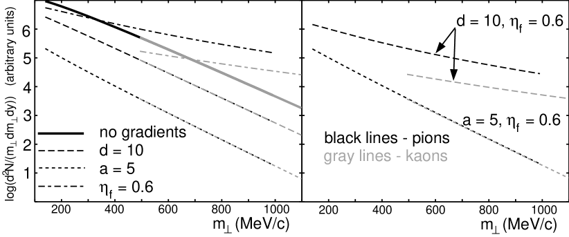
Figure 4: Transverse mass spectra at midrapidity from a transparent source. Black lines correspond to pions, gray lines to kaons. In the left plot the effects from different types of gradients are shown individually, in the right plot we study the interplay of transverse temperature gradients with transverse flow

shows the influence of transverse and temporal temperature gradients and of transverse flow on the $m_{\perp}$-spectra at fixed $Y_{{}_{\rm CM}}=0$. Qualitatively very similar features are seen at other rapidity values and in the rapidity integrated spectra. One sees that even very strong temporal and transverse temperature gradients do not cause any major effects on the single particle spectra, compared to the case without any gradients. Their main effect is a change of the normalisation because the colder regions of the emission function contribute less; their contribution is also concentrated at smaller momenta, leading to a somewhat steeper slope of the transverse mass spectra at low $m_{\perp}$.

This situation changes dramatically when the source develops transverse collective flow. In the absence of temperature gradients, transverse flow simply flattens the $m_{\perp}$-spectra [52]. For large $m_{\perp}\gg m_{0}$ (i.e. relativistic momenta) this can be described in terms of an effective blueshifted temperature $T_{\rm eff}=T\sqrt{{1+\langle v(r)\rangle\over 1-\langle v(r)\rangle}}$ which is the same for all particle species while at small $m_{\perp}$ the flattening is even stronger and depends on the particle mass via the nonrelativistic relation $T_{\rm eff}=T+m\langle v(r)\rangle^{2}$ [52]. These features have now been clearly observed in the heavy collision systems studied at the Brookhaven AGS and CERN SPS [53]. Transverse flow clearly also breaks the $m_{\perp}$ scaling between pions and kaons: the pion and kaon spectra in the left panel of Fig. 4 have different slopes and normalisations.

Additional temperature gradients which are imposed on top of the transverse expansion flow affect the spectra as shown in the right panel of Fig. 4. A temporal gradient of the source temperature has no qualitative effect on the shape of the $m_{\perp}$ spectra and only affects their normalisation. A transverse spatial gradient of the temperature, however, interferes seriously with the transverse flow by strongly reducing its effect on the slope of the $m_{\perp}$ spectra. For a strong transverse temperature gradient with $a=5$ as shown in the Figure, a comparison with the left panel shows that the flow effects become nearly invisible. An analytical discussion of this behaviour is given in [14] where it is shown to occur if the transverse homogeneity length generated by temperature gradient becomes much smaller than the one generated by the transverse velocity gradient. It follows from this discussion that it is not possible to generate a strong (additional) $M_{\perp}$-dependence of the transverse HBT radius parameter from transverse temperature gradients (see below) without at the same time reducing the flow effects on the single particle $m_{\perp}$ spectra.

We now proceed to a discussion of the HBT radius parameters. The effect of temporal temperature gradients is studied in Fig. 5.

Figure 5: The effects of temporal temperature gradients on the temporal YKP parameter $R_{0}$ (upper panel) and the difference $R^{2}_{o}-R^{2}_{s}$ in the Cartesian parametrisation (lower panel). Solid (dashed) lines are for pions (kaons). The calculations are done for midrapidity pairs, $Y_{{}_{\rm CM}}=0$, and for $a=\eta_{f}=0$

As expected, they affect mostly those HBT parameters which are sensitive to the effective lifetime of the source, namely the temporal YKP parameter $R_{0}$ and the Cartesian difference $R_{o}^{2}-R_{s}^{2}$. These are reduced by increasing $d$. The origin of this effect can be seen in Fig. 2 which shows that larger values of $d$ concentrate the high temperature region (with large emissivity) to a narrower region in the $z$-$t$ plane. The narrowing occurs predominantly in the temporal direction, but affects slightly also the longitudinal homogeneity length. Going from central rapidity to pairs at forward rapidities, all curves change in a similar way as shown in Fig. 3.

Transverse temperature gradients leave their traces only in the transverse homogeneity length measured by $R_{s}=R_{\perp}$. In Fig. 6

Figure 6: The effect of a transverse temperature gradient: The transverse radius parameter $R_{s}=R_{\perp}$ as a function of the transverse mass of the pair, for two different values of $a$. The coincidence of the solid (dashed) lines for pions (kaons) reflects the $M_{\perp}$-scaling of the transverse radius in this case. $d=\eta_{f}=0$, $Y_{{}_{\rm CM}}=0$

this is shown for pions and kaons at mid-rapidity. (Note that in our model $R_{s}$ is rapidity independent.)

The most important feature of both types of temperature gradients is that they do not break the $M_{\perp}$ scaling of the YKP correlation radii found in previous subsection. Note also that the temperature gradients have no qualitative impact on the YK rapidity $Y_{{}_{\rm YK}}$ associated with the YK velocity $v$.

Many of these features change in the presence of transverse flow. This is shown in Fig. 7

Figure 7: The correlation radii for a transparent source of constant temperature featuring transverse collective flow. The rapidity of the pairs was chosen as $Y_{{}_{\rm CM}}=1.5$. Left column: YKP radius parameters. Right column: Cartesian radius parameters. Solid (dashed) lines correspond to pions (kaons)

for pairs with rapidity $Y_{{}_{\rm CM}}=1.5$ in the CMS. All radius parameters have been calculated from space-time variances evaluated in the LCMS. The choice of a non-zero CMS pair rapidity ensures a non-vanishing cross term $R_{ol}$. The generic rapidity dependence of the radii follows the behaviour discussed in Sec. 4.1.

Since transverse flow introduces velocity gradients in the transverse direction, $R_{s}(=R_{\perp})$ and $R_{o}$ decrease with increasing $\eta_{f}$. Less obvious is, however, the rather strong effect of transverse flow on the “temporal” YKP parameter $R_{0}^{2}$. For higher transverse masses the latter even begins to increase with $M_{\perp}$. This does not, however, reflect the behaviour of the emission duration which continues to decrease for particles with higher $M_{\perp}$. The increase of $R_{0}^{2}$ is rather caused by correction terms expressing the difference between $R_{0}^{2}$ and the lifetime [20, 21]:

$$R_{0}^{2}-\langle{\tilde{t}}^{2}\rangle=\frac{2}{\beta_{\perp}}\langle\tilde{x}\tilde{t}\rangle+\frac{1}{\beta_{\perp}^{2}}\langle{\tilde{x}}^{2}-{\tilde{y}}^{2}\rangle\,.$$ (27)

Especially the second term on the r.h.s. grows appreciably with increasing $\eta_{f}$, and even more so for pions than for kaons. This was studied in detail in [21] (cf. Fig. 2 of that paper) where a more detailed explanation of the curves for $R_{0}^{2}$ shown here can be found.

The most important feature of Fig. 7 is the breaking of the $M_{\perp}$ scaling of the YKP radii by the transverse flow.

4.3 Interplay of all gradients

In [14] it was claimed that an interplay of the various types of gradients discussed above can lead to a common $1/\sqrt{M_{\perp}}$ scaling law for all three Cartesian HBT radii, $R_{l}$, $R_{s}$, and $R_{o}$, as well as for the effective lifetime of the source. The condition for such a common scaling is that the geometric extension is large compared to the “thermal length scales” generated by temperature and flow gradients [14]. The claim of [14] was based on approximate analytical expressions for these radius parameters which were obtained by evaluating the corresponding integrals over the emission function within an improved saddle-point approximation scheme. In this subsection we present a numerical test of this claim. To this end we select a set of parameters ($a=0.6$, $d=10$, $\eta_{f}=0.2$) for which at mid-rapidity the conditions for such a scaling, as given in [14], are satisfied as much as possible, without leaving the phenomenologically realistic range. It should be mentioned, that our model differs slightly from that of [14]. The differences are explicitly treated in Appendix A where they are shown to be small, and our findings are not affected by them.

The numerically evaluated correlation radii for this parameter set are plotted with thick black lines in Fig. 8.

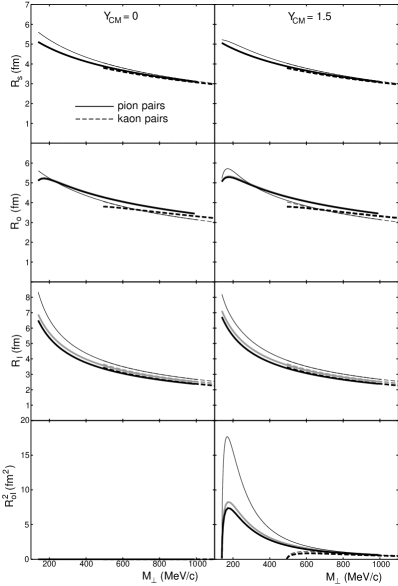
Figure 8: Correlation radii in the Cartesian parametrisation for a transparent source with parameters $a=0.6$, $d=10$, $\eta_{f}=0.2$. The thick black lines represent the exact result from a numerical evaluation of the space-time variances, the thick grey lines the result of numerical evaluation with the model of [14] with corresponding parameters (see Appendix A), the thin lines use the approximate analytical formulae given in [14]. Solid (dashed) lines are for pions (kaons). In cases of $R_{s}$ and $R_{o}$ thick black and grey lines overlap

The analytical approximation according to [14] is shown by the thin lines for comparison. With thick grey lines the numerically computed results from original model of [14] introduced in Appendix A are plotted. We agree with the conclusions drawn from a similar comparison presented in [23] that for kaons the approximate analytical formulae agree with the numerical curves within 15%. For pions with transverse momenta below 600 MeV the discrepancies are larger because one of the conditions of validity of the analytical formulae (sufficiently large $M_{\perp}$) is violated. However, the analytical approximation does not give at all the (slight) breaking of the $M_{\perp}$ scaling of $R_{l}$ by the transverse flow, and at mid-rapidity it misses the initial rise of $R_{o}$ at small $M_{\perp}$. This last point in particular is a serious problem if one wishes to extract an estimate of the effective lifetime according to Eq. (25). Similar (dis-)agreement at a comparative level is seen for forward rapidity pairs at $Y_{{}_{\rm CM}}=1.5$, with the exception of the cross term $R_{ol}$ which is strongly overestimated by the approximation. The analytical approximation of [14] is restricted by the condition that the flow rapidity of the point of maximum emissivity in the LCMS is small. Since the latter coincides with good approximation with the YK rapidity [20] and, in our model, the YK rapidity is found to converge to $Y$ in the limit $M_{\perp}\to\infty$ [20, 21], the point of maximum emissivity moves to zero LCMS rapidity in that limit. This explains why for large $M_{\perp}$ the analytical and numerical results agree.

On a superficial level the analytical approximations of [14] thus don’t seem to be doing too badly. We want to check, however, whether the results also confirm the suggested $1/\sqrt{M_{\perp}}$-scaling. In [21] it was shown that in general the strength of the $M_{\perp}$-dependence of $R_{s}$ and $R_{l}$ (resp. $R_{\perp}$ and $R_{\parallel}$) is correlated with the strength of collective flow in the transverse resp. longitudinal directions. One way of quantifying the strength of the $M_{\perp}$-dependence of the correlation radii is to fit them to a power law $R_{i}\propto M_{\perp}^{-\alpha_{i}}\ (i=s,l,\parallel,0)$ and to study the values of the exponents $\alpha_{i}$. According to the approximate formulae of [14], at mid-rapidity all these powers should be equal to 0.5. The $\alpha_{i}$-values obtained from the numerically evaluated correlation radii are listed in Table 3.

Table 3: The exponents $\alpha_{i}$ found in a fit of the numerically computed correlation radii to a power law $R_{i}\propto M_{\perp}^{-\alpha_{i}}$, for a source with the parameters given in Fig. 8

		$Y_{{}_{\rm CM}}$
		0	1.5	3
	pions	0.257	0.253	0.240
$\alpha_{s}$	kaons	0.306	0.304	0.297
	pions	0.512	0.527	0.565
$\alpha_{l}$	kaons	0.519	0.524	0.538
	pions	0.512	0.496	0.453
$\alpha_{\parallel}$	kaons	0.519	0.512	0.494
	pions	0.373	0.360	0.324
$\alpha_{0}$	kaons	0.225	0.223	0.262

One sees that only the longitudinal radius parameters (both in YKP and Cartesian parametrisations) follow an approximate $1/\sqrt{M_{\perp}}$ scaling law, similar to previous studies without temperature gradients [12, 21]. It reflects the boost-invariance of the longitudinal expansion velocity profile [9]. The transverse and temporal radius parameters $R_{s}=R_{\perp}$ and $R_{0}$ scale much more weakly with $M_{\perp}$. For mid-rapidity kaons $R_{0}$ provides a good estimate for the emission duration because for $\eta_{f}=0.2$ the correction terms on the r.h.s. of (27) are small; thus we find that also the effective lifetime of the source does not scale with $1/\sqrt{M_{\perp}}$. Thus, while the conditions for the saddle point approximation in [14] are satisfied with sufficient accuracy by our (semi-realistic) parameter set, the stronger conditions required for the common $1/\sqrt{M_{\perp}}$-scaling are not.

5 Conclusions

Let us shortly summarize the most important results:

Transverse temperature gradients and transverse flow have similar effects on the transverse HBT radii $R_{s}=R_{\perp}$, but not on the single particle spectra. Both lead to a decrease of $R_{s}$ with increasing $M_{\perp}$, but while transverse flow flattens the single particle spectra, a transverse temperature gradient only reduces their normalisation. A weak $M_{\perp}$-dependence of $R_{s}$ due to a moderate transverse flow can be increased by adding a transverse temperature gradient, but only at the expense of simultaneously reducing the flow effects on the single particle spectra. This is important for the interpretation of experimental data.

For transparent sources, transverse temperature gradients preserve the $M_{\perp}$-scaling of the YKP radius parameters while transverse flow breaks it. This breaking of $M_{\perp}$-scaling is weak, however, the most sensitive parameter being $R_{0}^{2}$.

Temporal temperature gradients affect mostly the temporal HBT radii, i.e. the difference $R_{o}^{2}-R_{s}^{2}$ in the Cartesian parametrisation and $R_{0}^{2}$ in the YKP parametrisation.

We could not confirm the existence of a common $1/\sqrt{M_{\perp}}$ scaling law for all three Cartesian HBT radius parameters and the effective source lifetime in the case of the “thermal lengths” being smaller than the geometric lengths. For realistic model parameters, the $M_{\perp}$-dependence for $R_{s}$ and $R_{0}$ is always much weaker than for the longitudinal radius parameters $R_{l}$ resp. $R_{\parallel}$.

Acknowledgements: We thank to Tamas Csörgő for very fruitful discussions which helped us to formulate the model study and comparison with analytical formulae more accurately. We are also indebted to Harry Appelshäuser, Ján Pišút, Claus Slotta, Axel Vischer and Urs Wiedemann for valuable and helpful comments. We acknowledge financial support by DAAD, DFG, BMBF, and GSI.

Appendix A The model of Csörgő and Lörstad

In this Appendix we point out the differences between our model and that of [14] and study their impact on our findings from Sec. 4.3.

The model of [14] is given by the emission function

$$S(x,K)\,d^{4}x = \frac{g}{(2\pi)^{3}}M_{\perp}\cosh(\eta-Y)\,\exp\left[-\frac{K\cdot u(x)}{T(x)}+\frac{\mu(x)}{T(x)}\right]$$ (28)

$$\times\;\frac{\tau_{0}^{\prime}\,d\tau}{\sqrt{2\pi\,{\Delta\tau^{\prime}}^{2}}}\exp\left[-\frac{(\tau-\tau_{0}^{\prime})^{2}}{2\,{\Delta\tau^{\prime}}^{2}}\right]\,d\eta\,r\,d\phi\,dr\,.$$

Since in the used coordinates the measure reads $d^{4}x=d\tau\,\tau\,d\eta\,r\,d\phi\,dr$, it is seen that here another geometric eigentime distribution is used, namely

$$H(\tau)=\frac{\tau_{0}^{\prime}}{\tau}\,\frac{1}{\sqrt{2\pi\,{\Delta\tau^{\prime}}^{2}}}\exp\left[-\frac{(\tau-\tau_{0}^{\prime})^{2}}{2\,{\Delta\tau^{\prime}}^{2}}\right]\,.$$ (29)

This differs from our distribution by the pre-factor ${\tau_{0}^{\prime}}/{\tau}$. For the comparison with our model, the values of ${\tau_{0}^{\prime}}$ and $\Delta\tau^{\prime}$ are obtained via the saddle point approximation to our Gaussian eigentime distribution multiplied by $\tau$ from the Jacobian. This gives

$$\tau_{0}^{\prime} = \frac{\tau_{0}+\sqrt{\tau_{0}^{2}+4\Delta\tau^{2}}}{2}\,,$$ (30)

$$\Delta\tau^{\prime} = \frac{\tau_{0}^{\prime}\,\Delta\tau}{\sqrt{\Delta\tau^{2}+{\tau_{0}^{\prime}}^{2}}}\,.$$ (31)

The remaining geometry of the model (28) is encoded in chemical potential

$$\frac{\mu(x)}{T(x)}=\frac{\mu_{0}}{T_{0}}-\frac{r^{2}}{2\,R^{2}}-\frac{(\eta-\eta_{0})^{2}}{2\,\Delta\eta^{2}}\,,$$ (32)

so this is the same as in our model (20). There is a slight difference in the formulation of temperature gradients:

$$\frac{1}{T(x)}=\frac{1}{T_{0}}\left(1+{a^{\prime}}^{2}\frac{r^{2}}{2\,{\tau_{0}^{\prime}}^{2}}\right)\left(1+{d^{\prime}}^{2}\frac{(\tau-\tau_{0}^{\prime})^{2}}{2\,{\tau_{0}^{\prime}}^{2}}\right)\,,$$ (33)

where the transverse gradient scales with ${a^{\prime}}/{\tau_{0}^{\prime}}$ (and not with $a/R$). Furthermore, the transverse flow rapidity is given as

$$\eta_{t}=\eta_{f}^{\prime}\frac{r}{\tau_{0}^{\prime}}\,,$$ (34)

instead of $\eta_{f}\,r/R$. This requires appropriate re-scaling of $a^{\prime}$ and $\eta_{f}^{\prime}$. Also, $d^{\prime}$ has to be re-scaled relatively to $d$ by the factor $\tau_{0}^{\prime}/\tau_{0}$. Note finally that in the numerical calculation we have used the expansion four-velocity field as given by the relativistic formula (21) with the transverse rapidity profile (34), while in [14] the non-relativistic approximation to the transverse expansion is used in the formulation of the model.

The results are plotted with grey lines in Fig. 8. It is clearly seen that the difference between the mentioned two models is small.

For the computation of the curves using the analytical formulae found in [14] (thin lines in Fig. 8) we used the re-scaled model parameters as explained above.

To be in the region where the $1/\sqrt{M_{\perp}}$-scaling should take place we have chosen: $a=0.6$, $d=10$, $\eta_{f}=0.2$. Note that with the appropriately re-scaled parameter values (see above) we satisfy the conditions given in [23] which need to be satisfied for a 15-20% agreement between the numerical calculation and the analytical approximations of the model (28).

To be sure that the slope parameters found in Table 3 are not an artefact of the difference between our model and that of [14] we did the same fit with the numerically calculated radii resulting from (28) and even with the analytically computed curves. Results of that fit are listed in Table 4.

Table 4: The exponents $\alpha_{i}$ found in a fit of the numerically computed correlation radii to a power law $R_{i}\propto M_{\perp}^{-\alpha_{i}}$, for a source from 28 and with the parameters correspondingly re-scaled to approximate those used in Fig. 8. In brackets are the results of the same fit done with curves computed using the analytical approximation from [14]

		$Y_{{}_{\rm CM}}$
		0	1.5	3
	pions	0.257 (0.301)	0.253 (0.274)	0.240
$\alpha_{s}$	kaons	0.306 (0.370)	0.304 (0.364)	0.297
	pions	0.511 (0.569)	0.526 (0.562)	0.564
$\alpha_{l}$	kaons	0.518 (0.531)	0.523 (0.535)	0.538
	pions	0.511	0.495	0.452
$\alpha_{\parallel}$	kaons	0.518	0.512	0.493
	pions	0.395	0.381	0.344
$\alpha_{0}$	kaons	0.245	0.242	0.279

The differences of the exponents listed in Tables 3 and 4 are in case of $\alpha_{s}$, $\alpha_{l}$ and $\alpha_{\parallel}$ within 1%, $\alpha_{0}$’s differ up to 10%. The qualitative discussion concerning the exponents from Sec. 4.3 remains valid for the set given in Table 4. The same is true for the analytically determined radii.

This again supports the conclusion, that even if good agreement between numerical and analytical results is achieved, for a realistic set of parameters the conditions for common scaling of all three Cartesian radii with $M_{\perp}^{-1/2}$ are not fulfilled.

References

-
[1]
R. Hanbury Brown and R.Q. Twiss, Phil. Mag. 45, 633 (1954);
and Nature 177, 27 (1956); 178, 1046 (1956); 178, 1447 (1956) - [2] G. Goldhaber, S. Goldhaber, W. Lee, and A. Pais, Phys. Rev. 120, 300 (1960)
- [3] M. Gyulassy, S.K. Kauffmann, and L.W. Wilson, Phys. Rev. C20, 2267 (1979)
- [4] B. Lörstad, Int. J. Mod. Phys. A12, 2861 (1989)
- [5] D. Boal, C.K. Gelbke and B. Jennings, Rev. Mod. Phys. 62, 553 (1990)
- [6] W.A. Zajc, in: Particle Production in Highly Excited Matter, edited by H.H. Gutbrod and J. Rafelski, (Plenum Press, New York, 1993), p. 435
- [7] S. Pratt, in: Quark-Gluon Plasma 2, edited by R.C. Hwa, (World Scientific Publ. Co., Singapore, 1995), p. 700
- [8] U. Heinz, in: Correlations and Clustering Phenomena in Subatomic Physics, edited by M.N. Harakeh, O. Scholten, and J.H. Koch, NATO ASI Series B, (Plenum, New York, 1997) (Los Alamos eprint archive nucl-th/9609029)
- [9] A.N. Makhlin and Y.M. Sinyukov, Z. Phys. C39, 69 (1988)
- [10] S. Chapman, P. Scotto, and U. Heinz, Phys. Rev. Lett. 74, 4400 (1995)
- [11] S. Chapman, P. Scotto, and U. Heinz, Heavy Ion Physics 1, 1 (1995)
- [12] U.A. Wiedemann, P. Scotto and U. Heinz, Phys. Rev. C53, 918 (1996)
- [13] T. Csörgő and B. Lörstad, Nucl. Phys. A590, 465c (1995)
- [14] T. Csörgő and B. Lörstad, Phys. Rev. C 54, 1390 (1996)
- [15] T. Csörgő and B. Lörstad, in Proceedings of XXV International Symposium on Multiparticle Dynamics, Sept. 12.-16. 1995, Stará Lesná, Slovakia, edited by D. Bruncko, L. Šándor and J. Urbán (World Scientific, Singapore, 1996), p. 661
- [16] S.V. Akkelin and Y.M. Sinyukov, Z. Phys. C72, 501 (1996)
- [17] H. Heiselberg and A.P. Vischer, Los Alamos eprint archive nucl-th/9609022
- [18] H. Heiselberg and A.P. Vischer, Los Alamos eprint archive nucl-th/9703030
- [19] B. Tomášik and U. Heinz, continuation of this paper containing study of opaque sources - work in progress
- [20] U. Heinz, B. Tomášik, U.A. Wiedemann, and Y.-F. Wu, Phys. Lett. B382, 181 (1996)
- [21] Y.-F. Wu, U. Heinz, B. Tomášik, and U.A. Wiedemann, Los Alamos eprint archive nucl-th/9607044, Z. Phys. C 77 (1997) in press
- [22] B. Tomášik, U. Heinz, U.A. Wiedemann, and Y.-F. Wu, Acta Phys. Slovaca 47, 81 (1997)
- [23] T. Csörgő, P. Lévai, and B. Lörstad, Acta Phys. Slovaca 46, 585 (1996)
- [24] T. Csörgő and B. Lörstad, Heavy Ion Physics 4, 221 (1996)
- [25] NA44 Coll., H. Beker et al., Phys. Rev. Lett. 74, 3340 (1995)
-
[26]
NA35 Coll., T. Alber et al., Z. Phys. C 66, 77 (1995);
NA35 Coll., T. Alber et al., Phys. Rev. Lett. 74, 1303 (1995) - [27] T. Alber, PhD thesis, MPI für Physik, München (1995), unpublished
- [28] T. Alber for the NA35 and NA49 Coll., Nucl. Phys. A 590, 453c (1995)
- [29] K. Kadija for the NA49 Coll., Nucl. Phys. A 610, 248c (1996)
- [30] S. Schönfelder, PhD thesis, MPI für Physik, München, 1996, unpublished
- [31] H. Appelshäuser, PhD thesis, Johann Wolfgang Goethe-Universität Frankfurt/Main, 1996, unpublished
- [32] S. Chapman, J.R. Nix, and U. Heinz, Phys. Rev. C52, 2694 (1995)
- [33] F. Yano and S. Koonin, Phys. Lett. B78, 556 (1978)
- [34] M.I. Podgoretskiĭ, Sov. J. Nucl. Phys. 37, 272 (1983)
- [35] J. Bolz et al., Phys. Lett. B300, 404 (1993); and Phys. Rev D47, 3860 (1993)
- [36] B.R. Schlei et al., Phys. Lett. B376, 212 (1996)
- [37] U. Ornik et al., Los Alamos eprint archive hep-ph/9604323
- [38] H. Heiselberg, Phys. Lett. B379, 27 (1996)
- [39] T. Csörgő, B. Lörstad, and J. Zimányi, Z. Phys. C71, 491 (1996)
- [40] U.A. Wiedemann and U. Heinz, Los Alamos eprint archive nucl-th/9611031, submitted to Phys. Rev. C
- [41] U.A. Wiedemann and U. Heinz, Los Alamos eprint archive nucl-th/9610043
- [42] U.A. Wiedemann and U. Heinz, Acta Phys. Slovaca 47, 95 (1997)
- [43] E. Shuryak, Phys. Lett. B44, 387 (1973); Sov. J. Nucl. Phys. 18, 667 (1974)
- [44] S. Pratt, Phys. Rev. Lett. 53, 1219 (1984); Phys. Rev. D33, 1314 (1986)
- [45] S. Chapman and U. Heinz, Phys. Lett. B340, 250 (1994)
- [46] M. Herrmann and G.F. Bertsch, Phys. Rev. C51, 328 (1995)
- [47] T. Csörgő and S. Pratt, in Proceedings of the Workshop on Relativistic Heavy Ion Physics at Present and Future Accelerators, Budapest, 1991, edited by T. Csörgő et al. (MTA KFKI Press, Budapest, 1991), p. 75
- [48] J.D. Bjorken, Phys. Rev. D27, 140 (1983)
- [49] U. Heinz, Nucl. Phys. A610, 264c (1996)
- [50] S. Chapman and J.R. Nix, Phys. Rev C54, 866 (1996)
- [51] U. Heinz, B. Tomášik, and U.A. Wiedemann, work in progress
- [52] K.S. Lee, U. Heinz, and E. Schnedermann, Z. Phys. C48, 525 (1990); E. Schnedermann, J. Sollfrank, and U. Heinz, Phys. Rev. C48, 2462 (1993)
- [53] Proceedings from Quark Matter ’96, (Heidelberg, 20.-24.5.1996), edited by P. Braun-Munzinger et al., Nucl. Phys. A 610 (1996)