Charm Quark Production in Non-central Heavy Ion Collisions

Abstract

The effect of gluon shadowing on charm quark production in large impact parameter ultrarelativistic heavy ion collisions is investigated. Charm production cross sections are calculated for a range of non-central impact parameters which can be accurately inferred from the global transverse energy distribution. We show that charm production is a good probe of the local parton density which determines the effectiveness of shadowing. The spatial dependence of shadowing can only be studied in heavy ion collisions.

(Submitted to Physical Review C.)

I Introduction

Deep inelastic scattering experiments using nuclear targets showed that the quark and antiquark distribution functions are modified in the nuclear environment [1] and hence are different in heavy nuclei than in free protons. It is not unreasonable to expect the nuclear gluon distributions to be affected at least as much as the quark distributions. However, little is known about the nuclear gluon distribution because the gluon distributions can only be indirectly probed. Gluon-dominated production processes, such as $J/\psi$ and heavy quark production, can provide an indirect measure of the nuclear gluon distribution. Since the $J/\psi$ is more strongly affected by absorption processes than charm quarks, evident from their respective $A$ dependencies [2, 3], charmed quark production provides a cleaner determination of the nuclear gluon distribution.

To date, all measurements and indirect determinations of nuclear parton distributions have been insensitive to the position of the interacting parton within the nucleus. However, there is no reason to expect the parton momentum distributions to be constant within the nucleus. They should at least vary with the local nuclear density. If shadowing is due to gluon recombination, the position dependence could be quite strong [4]. One way to probe the position dependence of the shadowing is to measure $c\overline{c}$ production over a wide range of impact parameters, thus scanning gluon localization in the nucleus. The charm rate has been shown to be large in central collisions [5], here we will show that these studies are also feasible at large impact parameters.

This paper thus proposes a method for measuring the position dependence of the gluon momentum distribution in heavy nuclei. We show that the charm production rates in non-central collisions are sensitive to the details of the gluon distribution and its position dependence. We use two different parameterizations of nuclear shadowing along with two parameterizations of the position dependence of the shadowing to calculate charm production in 100 GeV per nucleon Au+Au collisions at the Relativistic Heavy Ion Collider (RHIC)[6], now under construction at Brookhaven National Laboratory. However, the techniques discussed here should also be applicable to $c\overline{c}$ and $b\overline{b}$ production in Pb+Pb collisions at the CERN Large Hadron Collider (LHC). The charm quark production rate and $p_{T}$ spectra are calculated as a function of impact parameter, $b$, for non-central collisions with impact parameters greater than the nuclear radius, $R_{A}$.

For this study, we need to select events according to impact parameter. Although the impact parameter of the collision is not directly measurable, it may be inferred from the total transverse energy, $E_{T}$, of the event[7]. We discuss the relationship between $E_{T}$ and $b$ and present calculations showing that, for a given $E_{T}$, the impact parameter can be measured relatively accurately. Additional input, such as a measurement of nuclear breakup, through the use of a zero degree calorimeter, can refine this estimate.

Section 2 summarizes the calculations of $c\overline{c}$ production in peripheral collisions including a discussion of the nuclear parton shadowing and its possible spatial dependence. Section 3 discusses the relationship between transverse energy and impact parameter. Section 4 presents the numerical results for the charm production rates and $p_{T}$ spectra for two ranges of non-central impact parameters. We demonstrate how these rates are sensitive to the nuclear gluon distribution. Our results are put into an experimental perspective in Section 5. Finally, Section 6 draws some conclusions.

II $c\overline{c}$ Production

To study the effects of shadowing on $c\overline{c}$ production in peripheral collisions, we emphasize the modifications of the parton distribution functions due to shadowing as well as the location of the interacting parton in the nucleus. We discuss the method used to calculate $c\overline{c}$ pair production and introduce two parameterizations of nuclear shadowing. We also describe two models of the spatial dependence of the shadowing.

The double differential cross section for $c\overline{c}$ pair production by nuclei $A$ and $B$ is

$$E_{c}E_{\overline{c}}\frac{d\sigma_{AB}}{d^{3}p_{c}d^{3}p_{\overline{c}}d^{2}bd^{2}r}=$$ (2)

$$\sum_{i,j}\int\,dz\,dz^{\prime}\,dx_{1}\,dx_{2}F_{i}^{A}(x_{1},Q^{2},\vec{r},z)F_{j}^{B}(x_{2},Q^{2},\vec{b}-\vec{r},z^{\prime})E_{c}E_{\overline{c}}\frac{d\widehat{\sigma}_{ij}(x_{1}P_{1},x_{2}P_{2},m_{c},Q^{2})}{d^{3}p_{c}d^{3}p_{\overline{c}}}\,\,.$$

Here $i$ and $j$ are the interacting partons in the nucleus and the functions $F_{i}$ are the number densities of gluons, light quarks and antiquarks evaluated at momentum fraction $x$, scale $Q^{2}$, and location $\vec{r}$, $z$. (Note that $\vec{r}$ is two-dimensional.) The short-distance cross section, $\widehat{\sigma}_{ij}$, is calculable as a perturbation series in $\alpha_{s}(Q^{2})$.

At leading order (LO), $c\overline{c}$ production proceeds by two basic processes,

$$q+\overline{q} \rightarrow c+\overline{c}$$ (3)

$$g+g \rightarrow c+\overline{c}\,\,.$$ (4)

The LO cross section, ${\cal O}(\alpha_{s}^{2})$, can be written as

$$E_{c}E_{\overline{c}}\frac{d\sigma_{AB}}{d^{3}p_{c}d^{3}p_{\overline{c}}d^{2}bd^{2}r}=$$ (6)

$$\int\frac{s}{2\pi}\,dz\,dz^{\prime}\,dx_{1}\,dx_{2}\,C(x_{1},x_{2},Q^{2},\vec{r},z,\vec{b}-\vec{r},z^{\prime})\,\delta^{4}(x_{1}P_{1}+x_{2}P_{2}-p_{c}-p_{\overline{c}})\,\,$$

where $\sqrt{s}$, the parton-parton center-of-mass energy, is related to $\sqrt{S}$, the hadron-hadron center-of-mass energy, by $s=x_{1}x_{2}S\geq 4m_{c}^{2}$, where the momentum fractions, $x_{1}$ and $x_{2}$, are

$$x_{1,2}=\frac{m_{T}}{\sqrt{s}}(e^{\pm y}+e^{\pm\overline{y}})\,\,,$$ (7)

and $m_{T}=\sqrt{m_{c}^{2}+p_{T}^{2}}$. The target fraction, $x_{2}$, decreases with rapidity while the projectile fraction, $x_{1}$, increases. Here, the intrinsic transverse momenta of the incoming partons has been neglected. The convolution of the subprocess cross sections with the parton number densities is contained in $C(x_{1},x_{2},Q^{2},\vec{r},z,\vec{b}-\vec{r},z^{\prime})$ where

$$C(x_{1},x_{2},Q^{2},\vec{r},z,\vec{b}-\vec{r},z^{\prime})=$$ (10)

$$\sum_{q}[F_{q}^{A}(x_{1},Q^{2},\vec{r},z)F_{\overline{q}}^{B}(x_{2},Q^{2},\vec{b}-\vec{r},z^{\prime})+F_{\overline{q}}^{A}(x_{1},Q^{2},\vec{r},z)F_{q}^{B}(x_{2},Q^{2},\vec{b}-\vec{r},z^{\prime})]\frac{d\widehat{\sigma}_{q\overline{q}}}{dt}$$

$$+F_{g}^{A}(x_{1},Q^{2},\vec{r},z)F_{g}^{B}(x_{2},Q^{2},\vec{b}-\vec{r},z^{\prime})\frac{d\widehat{\sigma}_{gg}}{dt}\,\,.$$

Four-momentum conservation leads to the rather simple expression

$$\frac{d\sigma_{AB}}{dp_{T}^{2}dyd\overline{y}d^{2}bd^{2}r}=\int dz\,dz^{\prime}\,x_{1}x_{2}C(x_{1},x_{2},Q^{2},\vec{r},z,\vec{b}-\vec{r},z^{\prime})\,\,,$$ (11)

The LO subprocess cross sections for $c\overline{c}$ production by $q\overline{q}$ annihilation and $gg$ fusion, expressed as a function of $m_{T}$, $y$, and $\overline{y}$, are [9]

$$\frac{d\hat{\sigma}_{q\overline{q}}}{dt}=\frac{\pi\alpha_{s}^{2}}{9m_{T}^{4}}\frac{\cosh(y-\overline{y})+m_{c}^{2}/m_{T}^{2}}{(1+\cosh(y-\overline{y}))^{3}}\,\,,$$ (12)

$$\frac{d\hat{\sigma}_{gg}}{dt}=\frac{\pi\alpha_{s}^{2}}{96m_{T}^{4}}\frac{8\cosh(y-\overline{y})-1}{(1+\cosh(y-\overline{y}))^{3}}\left(\cosh(y-\overline{y})+\frac{2m_{c}^{2}}{m_{T}^{2}}-\frac{2m_{c}^{4}}{m_{T}^{4}}\right)\,\,.$$ (13)

Leading order calculations tend to underestimate the measured charm production cross section by a constant factor, usually called a $K$ factor,

$$K_{\rm exp}^{\rm LO}=\frac{\sigma_{\rm exp}(AB\rightarrow c\overline{c})}{\sigma_{\rm LO}(AB\rightarrow c\overline{c})}\,\,,$$ (14)

The next-to-leading order (NLO) corrections to the LO cross section have been calculated [10, 11] and an analogous theoretical $K$ factor $K_{\rm th}$ can be defined from the ratio of the NLO to the LO cross sections,

$$K_{\rm th}=\frac{\sigma_{\rm NLO}(AB\rightarrow c\overline{c})}{\sigma_{\rm LO}(AB\rightarrow c\overline{c})}\,\,,$$ (15)

where $\sigma_{\rm NLO}$ is the sum of the LO cross section and the ${\cal O}(\alpha_{s})$ corrections.

Previously [12], the NLO calculations were compared to the $c\overline{c}$ total production cross section data to fix $m_{c}$ and $Q$ so that $K_{\rm exp}^{\rm NLO}\sim 1$ to provide a more reliable estimate for nuclear collider energies. Reasonable agreement with the measured total cross section was found for $m_{c}=1.2$ GeV, $Q=2m_{c}$ for MRS D$-^{\prime}$ [13] and $m_{c}=1.3$ GeV, $Q=m_{c}$ for GRV HO [14]. We choose different scales for the two sets because of the different initial scales of the two parton distributions. The MRS D$-^{\prime}$ distributions have $Q_{0,{\rm MRS}}^{2}=5$ GeV²; we choose $Q=2m_{c}$ so that $Q^{2}>Q_{0,{\rm MRS}}^{2}$. The GRV HO sea quark and gluon distributions are valence-like at low $x$ and $Q_{0,{\rm GRV}}^{2}=0.3$ GeV². We can then use $Q=m_{c}$ because $m_{c}^{2}>Q_{0,{\rm GRV}}^{2}$. However, below $Q^{2}\approx 5$ GeV² the gluon distribution is still somewhat valence-like.

When calculating inclusive distributions rather than total cross sections, it is more appropriate to choose $Q\propto m_{T}$, particularly when $p_{T}>m_{c}$ since a constant scale introduces unregulated collinear divergences [16]. Therefore, we take $Q=2m_{T}$ for the MRS D$-^{\prime}$ distributions and $Q=m_{T}$ for the GRV HO distributions. Both sets of parton densities result in a NLO total $c\overline{c}$ production cross section of $\sim 350$ $\mu$b in $pp$ collisions at $\sqrt{s}=200$ GeV.

The differential $K_{\rm th}$ for the charm quark $p_{T}$ distribution, the pair mass distribution, and the charm quark and $c\overline{c}$ pair rapidity distributions are nearly constant at RHIC energy[16]. They are also essentially independent of the parton density. The value of $K_{\rm th}$ is determined by a comparison of the NLO and LO total cross sections. Our LO calculations, eq. (4), are multiplied by the appropriate $K_{\rm th}$ found for the specific parton density: 2.5 for the MRS D$-^{\prime}$ distributions and 2.9 for the GRV HO distributions.

The nucleon parton densities are only a part of the space-dependent nuclear number densities, $F_{i}^{A}(x,Q^{2},\vec{r},z)$, introduced in eq. (1). We have assumed that these nuclear number densities factorize into nuclear density distributions, independent of $x$ and $Q^{2}$, the nucleon parton densities, independent of spatial position and $A$, and a shadowing function that parameterizes the modifications of the nucleon parton densities in the nucleus, dependent on $x$, $Q^{2}$, $A$ and location,

$$F_{i}^{A}(x,Q^{2},\vec{r},z) = \rho_{A}(s)S^{i}(A,x,Q^{2},\vec{r},z)f_{i}^{p}(x,Q^{2})$$ (16)

$$F_{i}^{B}(x,Q^{2},\vec{b}-\vec{r},z^{\prime}) = \rho_{B}(s^{\prime})S^{i}(B,x,Q^{2},\vec{b}-\vec{r},z^{\prime})f_{i}^{p}(x,Q^{2})\,\,,$$ (17)

where $s=\sqrt{r^{2}+z^{2}}$, $s^{\prime}=\sqrt{|\vec{b}-\vec{r}|^{2}+z^{\prime\,2}}$ and $f_{i}^{p}$ are the nucleon parton densities. We assume that $z$ and $z^{\prime}$ are uncorrelated. The collision geometry in the plane transverse to the beam is shown in Fig. 1.

A three parameter Wood–Saxon shape is used to describe the nuclear density distribution,

$$\rho_{A}(s)=\rho_{0}\frac{1+\omega(s/R_{A})^{2}}{1+\exp((s-R_{A})/d)}\,\,,$$ (18)

where $R_{A}$ is the nuclear radius, $d$ is the surface thickness, and $\omega$ allows for central irregularities. The electron scattering data of Ref. [17] is used for $R_{A}$, $d$, and $\omega$ assuming that the charge and matter density distributions are identical. The central density, $\rho_{0}$, is found from the normalization $\int d^{2}rdz\rho_{A}(s)=A$. For gold, $\omega=0$, $d=0.535$ fm, $R_{A}=6.38$ fm, and $\rho_{0}=0.1693$ fm^-3.

If the parton densities in the nucleon and in the nucleus are the same, then $S^{i}(A,x,Q^{2},\vec{r},z)\equiv 1$. We will use this as a baseline against which to compare our results with shadowing included.

We now discuss our choices of the shadowing parameterizations used in our calculations, independent of the position. Measurements of the nuclear charged parton distributions by deep-inelastic scattering on a nuclear target and a deuterium target, show that the ratio $R_{F_{2}}=F_{2}^{A}/F_{2}^{D}$ has a characteristic shape as a function of $x$. The region below $x\sim 0.1$ is referred to as the shadowing region and the region $0.3<x<0.7$ is known as the EMC region. In both regions a depletion is observed in the heavy nucleus relative to deuterium and $R_{F_{2}}<1$. At very low $x$, $x\approx 0.001$, $R_{F_{2}}$ appears to saturate [19]. Between the shadowing and EMC regions, an enhancement, antishadowing, occurs where $R_{F_{2}}>1$. There is also an enhancement as $x\rightarrow 1$, assumed to be due to Fermi motion of the nucleons. The general behavior of $R_{F_{2}}$ as a function of $x$ is often referred to as shadowing. Although this behavior is not well understood for all $x$, the shadowing effect can be modeled by an $A$ dependent fit to the nuclear deep-inelastic scattering data and implemented by a modification of the parton distributions in the proton. We use two different models of the relation between $R_{F_{2}}$ and $S^{i}(A,x,Q^{2})$. These two parameterizations were used earlier to estimate the effect of shadowing on $c\overline{c}$ and $b\overline{b}$ production in central collisions [5] with no spatial dependence assumed for the shadowing.

The first parameterization is a fit to recent nuclear deep-inelastic scattering data. The fit does not differentiate between quark, antiquark, and gluon modifications and does not include evolution in $Q^{2}$. Therefore it is not designed to conserve baryon number or momentum. We define $R_{F_{2}}=S_{1}(A,x)$ [20] with

$$S_{1}(A,x)=\left\{\begin{array}[]{ll}R_{s}{\displaystyle\frac{1+0.0134(1/x-1/x_{\rm sh})}{1+0.0127A^{0.1}(1/x-1/x_{\rm sh})}}&\mbox{$x<x_{\rm sh}$}\\ a_{\rm emc}-b_{\rm emc}x&\mbox{$x_{\rm sh}<x<x_{\rm fermi}$}\\ R_{f}\bigg{(}{\displaystyle\frac{1-x_{\rm fermi}}{1-x}}\bigg{)}^{0.321}&\mbox{$x_{\rm fermi}<x<1$}\end{array}\right.\,\,,$$ (22)

where $R_{s}=a_{\rm emc}-b_{\rm emc}x_{\rm sh}$, $R_{f}=a_{\rm emc}-b_{\rm emc}x_{\rm fermi}$, $b_{\rm emc}=0.525(1-A^{-1/3}-1.145A^{-2/3}+0.93A^{-1}+0.88A^{-4/3}-0.59A^{-5/3})$, and $a_{\rm emc}=1+b_{\rm emc}x_{\rm emc}$. The fit fixes $x_{\rm sh}=0.15$, $x_{\rm emc}=0.275$ and $x_{\rm fermi}=0.742$. Thus, the nuclear parton densities are modified so that

$$f_{i}^{A}(x,Q^{2}) = S_{1}(A,x)f_{i}^{p}(x,Q^{2}).$$ (23)

The second parameterization, $S_{2}^{i}(A,x,Q^{2})$, modifies the valence and sea quark and gluon distributions separately and also includes $Q^{2}$ evolution[21], but is based on an older fit to the data using the Duke-Owens parton densities [22]. The initial scale for the evolution is $Q_{0}=2$ GeV and the $Q^{2}$ evolution is studied with both the standard Altarelli-Parisi evolution and with modifications due to gluon recombination at high density. The gluon recombination terms do not strongly alter the evolution. In this case, the nuclear parton densities are modified so that

$$f_{V}^{A}(x,Q^{2}) = S_{2}^{V}(A,x,Q^{2})f_{V}^{p}(x,Q^{2})$$ (24)

$$f_{S}^{A}(x,Q^{2}) = S_{2}^{S}(A,x,Q^{2})f_{S}^{p}(x,Q^{2})$$ (25)

$$f_{G}^{A}(x,Q^{2}) = S_{2}^{G}(A,x,Q^{2})f_{G}^{p}(x,Q^{2})\,\,,$$ (26)

where $f_{V}=u_{V}+d_{V}$ is the valence quark density and $f_{S}=2(\overline{u}+\overline{d}+\overline{s})$ is the total sea quark density. We assume that $S_{2}^{V}$ and $S_{2}^{S}$ affect the up, down, and strange valence and sea quarks identically. The ratios were constrained by assuming that $R_{F_{2}}\approx S_{2}^{V}$ at large $x$ and $R_{F_{2}}\approx S_{2}^{S}$ at small $x$ since $xf_{V}^{p}(x,Q_{0}^{2})\rightarrow 0$ as $x\rightarrow 0$. For the gluons, we take $R_{F_{2}}\approx S_{2}^{G}$ for all $x$ [21], since one might expect more shadowing for the sea quarks, generated from gluons, at small $x$. These parton densities do conserve baryon number, $\int_{0}^{1}dx\,f_{V}^{p,A}(x,Q^{2})=3$, and momentum, $\int_{0}^{1}dx\,x(f_{V}^{p,A}(x,Q^{2})+f_{S}^{p,A}(x,Q^{2})+f_{G}^{p,A}(x,Q^{2}))=1$. at all $Q^{2}$. We have used the MRS D$-^{\prime}$ and GRV HO densities with $S_{2}^{i}$ instead of the Duke-Owens densities, leading to some small deviations in the momentum sum but the general trend is unchanged.

Since the shadowing is likely related to the nuclear density, it should also depend on the spatial distribution of the partons within the nucleus so that $S^{i}(A,x,Q^{2},\vec{r},z)\rightarrow 1$ as $s\rightarrow\infty$. The reduced shadowing is reasonable since the shadowing mechanism should be less effective when the nuclear density is low. This spatial dependence should also be normalized so that $\frac{1}{A}\int d^{2}rdz\rho(s)S^{i}(A,x,Q^{2},\vec{r},z)=S^{i}(A,x,Q^{2})$ to recover the deep-inelastic scattering results which do not have any explicit impact parameter dependence. This approach may fail when $x\rightarrow 1$, because then the change in the structure function is likely due to Fermi motion, which should not exhibit spatial dependence.

One natural parameterization of the spatial dependence follows the nuclear matter density distribution,

$$S^{i}_{\rm WS}=S^{i}(A,x,Q^{2},\vec{r},z) = 1+N_{\rm WS}\frac{S^{i}(A,x,Q^{2})-1}{1+\exp((s-R_{A})/d)}$$ (27)

$$= 1+N_{\rm WS}(S^{i}(A,x,Q^{2})-1)\frac{\rho(s)}{\rho_{0}}\,\,,$$ (28)

where $N_{\rm WS}=1.317$ is needed for the normalization to $S^{i}(A,x,Q^{2})$. This form of the spatial dependence has a rather weak dependence on $s$ until the nuclear surface is approached. Note that when $s\rightarrow 0$, $S^{i}_{\rm WS}<S^{i}$ in the shadowing and EMC regions while $S^{i}_{\rm WS}>S^{i}$ in the antishadowing region.

The actual spatial dependence of shadowing may be stronger if the shadowing effect is not directly related to the nuclear matter density distribution. This can occur if the gluons are not well localized within the nucleus. One can alternatively assume that the shadowing is related to the nuclear thickness at the collision point, proportional to the distance a parton from one nucleus travels through the other [23]. Therefore we also consider

$$S^{i}_{\rm R}(A,x,Q^{2},\vec{r},z)=\left\{\begin{array}[]{ll}1+N_{\rm R}(S^{i}(A,x,Q^{2})-1)\sqrt{1-(r/R_{A})^{2}}&\mbox{$r\leq R_{A}$}\\ 1&\mbox{$r>R_{A}$}\end{array}\right.\,\,,$$ (31)

where $N_{\rm R}=1.449$ assures the normalization after the average over $\rho(s)$. Similarly, when $s\rightarrow 0$, $S^{i}_{\rm R}<S^{i}$ in the shadowing and EMC regions while $S^{i}_{\rm R}>S^{i}$ in the antishadowing region. The normalization is higher here because of the larger region over which the suppression due to shadowing is reduced relative to $S^{i}_{\rm WS}$.

We calculate the $c\overline{c}$ production cross sections in peripheral nuclear collisions with $S^{i}(A,x,Q^{2})=1$, $S_{1}$, and $S_{2}^{i}$. As we will show, the shape of the inclusive charm quark $p_{T}$ distributions are similar for $S_{1}$ and $S_{2}^{i}$. Therefore, we model the spatial dependence of $S_{1}$ only, according to eqs. (19) and (20).

III Correlation between E_T and impact parameter

Although the impact parameter is not directly measurable it can be related to direct observables. We discuss here the indirect measurement of the impact parameter $b$ by means of the transverse energy $E_{T}$ [7, 24]. Here $E_{T}=\Sigma_{i}\sqrt{m_{i}^{2}+p_{Ti}^{2}}$, summed over all detected particles in the event with masses $m_{i}$ and transverse momenta $p_{Ti}$. It is also possible to infer the impact parameter by a measurement of the nuclear breakup since the beam remnants deposited in a zero degree calorimeter are correlated with the impact parameter. A measure of the total charged particle multiplicity, proportional to $E_{T}$, could be used to refine the impact parameter determination.

The transverse energy contains “soft” and “hard” components. The “hard” components arise from quark and gluon interactions above momentum $p_{0}$, the scale above which perturbative QCD is assumed to be valid. Minijet production, calculated for $p_{T,{\rm jet}}>p_{0}\sim 2$ GeV [25], becomes an important contribution to the dynamics of the system in high-energy nucleus-nucleus collisions. The hard cross section, $\sigma_{H}^{pp}(p_{0})=2\sigma_{\rm jet}$, twice the single LO minijet production cross section, can be calculated perturbatively. “Soft” processes with $p_{T}<p_{0}$ are not perturbatively calculable yet they produce a substantial fraction of the measured $E_{T}$ at high energies (and almost the entire $E_{T}$ at CERN SPS energies). These processes must be modeled phenomenologically. We assume $\sigma_{S}^{pp}=\sigma_{\rm inelastic}^{pp}$, the inelastic $pp$ scattering cross section. Our calculation of the total $E_{T}$ distribution follows Ref. [24].

If the hard component is formed by independent parton-parton collisions, then the average number of hard parton-parton collisions as a function of $b$, $N_{AA}^{H}(b)$, is

$$\overline{N}_{AA}^{H}(b)=T_{AA}(b)\sigma^{pp}_{H}(p_{0})\,\,,$$ (32)

where $\sigma^{pp}_{H}(p_{0})\sim 6.5$ mb at RHIC [25] and $T_{AA}(b)$ is the nuclear overlap function,

$$T_{AA}(b)=\int d^{2}rT_{A}(\vec{r})T_{A}(\vec{b}-\vec{r})$$ (33)

where the nuclear thickness function is defined as $T_{A}(\vec{r})=\int dz\rho_{A}(z,\vec{r})$. In Au+Au collisions at $b=0$, $T_{AA}=29$/mb [26]. The $E_{T}$ distribution can be expressed as [24]

$${d\sigma_{H}\over dE_{T}}=\int d^{2}b{\Sigma}_{N=1}^{\infty}{[\overline{N}_{AA}^{H}(b)]^{N}\over N!}\exp{[-\overline{N}_{AA}^{H}(b)]}\int\prod_{i=1}^{N}dE_{Ti}{1\over\sigma^{pp}_{H}}{d\sigma^{pp}_{H}\over dE_{Ti}}\delta(E_{T}-{\Sigma}_{i=1}^{N}E_{Ti})\,\,.$$ (34)

If $\overline{N}_{AA}^{H}$ is large, $d\sigma_{H}/dE_{T}$ can be approximated by the Gaussian [24]

$${d\sigma_{H}\over dE_{T}}=\int d^{2}b{1\over\sqrt{2\pi\sigma^{2}_{H}(b)}}\exp{\bigg{(}\,-\,{(E_{T}-\overline{E}_{T\,H}^{AA}(b))^{2}\over 2\sigma^{2}_{H}(b)}\bigg{)}},$$ (35)

where the mean $E_{T}$, $\overline{E}_{T\,H}^{AA}(b)$, and standard deviation, $\sigma_{H}(b)$, are proportional to the first and second $E_{T}$ moments of the hard cross section,

$$\overline{E}_{T\,H}^{AA}(b) = T_{AA}(b)\sigma^{pp}_{H}(p_{0})\langle E_{T}\rangle^{pp}_{H}$$ (36)

$$\sigma^{2}_{H}(b) = T_{AA}(b)\sigma^{pp}_{H}(p_{0})\langle E_{T}^{2}\rangle^{pp}_{H}\,\,.$$ (37)

In the rapidity interval $|y|\leq 0.5$, $\sigma^{pp}_{H}(p_{0})\langle E_{T}\rangle^{pp}_{H}\approx 17\,{\rm mb\ GeV}$ and $\sigma^{pp}_{H}(p_{0})\langle E_{T}^{2}\rangle^{pp}_{H}\approx 70\,{\rm mb\ GeV}^{2}$ [25].

At RHIC energies, the hard part does not dominate the soft component, proportional to the number of nucleon-nucleon collisions,

$$\overline{N}_{AA}^{S}(b)=T_{AA}(b)\sigma^{pp}_{S}\,\,,$$ (38)

where $\sigma^{pp}_{S}\sim 30$ mb. Since the soft component is almost independent of the collision energy, we assume, as in Ref. [24], that the hard and soft components are separable on the $pp$ level and thus independent of each other at fixed $b$. Therefore the total $E_{T}$ distribution is a convolution of the hard and soft components with total mean and standard deviation

$$\overline{E}_{T}^{AA}(b) = T_{AA}(b)[\sigma^{pp}_{H}(p_{0})\langle E_{T}\rangle^{pp}_{H}+\epsilon_{0}]$$ (39)

$$\sigma^{2}(b) = T_{AA}(b)[\sigma^{pp}_{H}(p_{0})\langle E_{T}^{2}\rangle^{pp}_{H}+\epsilon_{1}]$$ (40)

where $\epsilon_{0}$ and $\epsilon_{1}$ are taken from lower energy data and adjusted to the same rapidity interval as the hard component, $|y|\leq 0.5$, $\epsilon_{0}=15$ mb GeV, $\epsilon_{1}=50$ mb GeV² [24]. Shadowing, which affects the hard component by reducing the minijet cross section, is not included in these averages. Multiplying $\sigma^{pp}_{H}$ by a shadowing factor modifies the $E_{T}$ distribution by less than 10% [27]. A correction has been included here.

Figure 2 shows the $E_{T}$ distribution (for $y<|0.5|$) for 100 GeV/nucleon Au+Au collisions for several different impact parameter intervals as well as the total cross section. Singling out a particular $E_{T}$ range can therefore select a rather narrow distribution of impact parameters. For example, requiring $E_{T}<300$ GeV selects almost exclusively events with $b>R_{A}$ while $E_{T}<180$ GeV selects events with $b>1.2R_{A}$.

Good event purity can be obtained with even narrower selections. For example, 300 GeV $>E_{T}>180$ GeV largely corresponds to $1.2R_{A}>b>R_{A}$. An example of the purity can be seen in Fig. 3 which shows the range of impact parameters at $E_{T}=200$ GeV. The distribution is centered at $b=1.27R_{A}$ with a standard deviation $\sigma\sim 0.05R_{A}$. Approximately 90% of the events fall into the range $1.15R_{A}<b<1.35R_{A}$, narrow enough to be an effective impact parameter selector. Thus at $E_{T}=200$ GeV, the impact parameter can be measured to within 10%. However, the statistical accuracy depends on the average number of collisions, proportional to $E_{T}$, so that $\sigma/b\approx 1/\sqrt{E_{T}}$.

For very small $E_{T}$, complications arise. The first concerns the transition from eq. (23) to eq. (24) which is only valid if $\overline{N}_{AA}^{H}(b)$ is large enough for the Poisson distribution to be approximated by a Gaussian. For a small number of collisions, eq. (24) overestimates the number of low $E_{T}$ events, even allowing a finite probability for negative $E_{T}$ events. In practice, the agreement is quite good even at $b=1.8R_{A}$, corresponding to $T_{AA}=0.9$/mb, $N_{AA}^{H}=5.5$ and $E_{T}\approx 30$  GeV. At significantly smaller $E_{T}$ a correction is needed. Further, the event by event fluctuations are large when the collision number is small, increasing the uncertainty in the impact parameter measurement.

At small $E_{T}$ the presence of charmed quarks will alter the relationship between $E_{T}$ and impact parameter because a $c\overline{c}\rightarrow D\overline{D}$ pair must have $E_{T}>2m_{D}\approx 3.7$ GeV. Typical values are $E_{T}\sim 4-6$ GeV. Thus when $E_{T}<20$ GeV, the relationship between $E_{T}$ and $b$ in charm events will be different. This altered relationship can be studied in simulations to correct the data.

Finally, other types of interactions can contribute to charm production at low $E_{T}$. The largest identified charm contribution in very peripheral collisions is photon-gluon fusion [8, 28].

Any real detector can only measure $E_{T}$ in a limited rapidity interval. For example, the calorimeter of the STAR detector at RHIC will cover the range $-1<y<2$[29]. The acceptance can be compensated by appropriately modifying $\langle E_{T}\rangle^{pp}_{H}$, $\langle E_{T}^{2}\rangle^{pp}_{H}$, $\epsilon_{0}$ and $\epsilon_{1}$, given here for $|y|<0.5$. The accuracy scales roughly as the square root of the observed energy. A large acceptance can also extend the region of validity of eq. (24) to larger $b$.

The non-central event selection technique to constrain the impact parameter may be useful in other analyses of heavy ion data. At large impact parameters, only the outer portions of the nuclei are involved but as the collision centrality increases, the nuclear interior is more deeply probed. Therefore the impact parameter variation roughly corresponds to the portion of the nucleus involved in the interaction, and can thus be used to study the difference between the parton constituents of the nuclear core and those near the surface.

IV Results

The best way to determine the gluon momentum fraction is to detect both charm quarks. Then $x_{1}$ and $x_{2}$ can be fixed exactly and the shadowing mapped out. The measurements are relatively easy to interpret if $y=-\overline{y}$ since $x_{1}=x_{2}$. After first discussing the general results when the kinematic variables are integrated over, we show the $p_{T}$ distributions for the MRS D$-^{\prime}$ and GRV HO parton densities assuming both the $c$ and $\overline{c}$ are detected. The low experimental efficiency for detecting charm suggests that it is unlikely for both quarks to be detected in an event. Thus we subsequently discuss the feasibility of the study if only one of the charm quarks is detected.

Figure 4 shows the $c\overline{c}$ production cross section as a function of impact parameter for $b>R_{A}$ with $S=1$, $S_{1}$ and $S_{2}$ at RHIC[6]. The cross sections were calculated by integrating eq. (1) over the $c$ and $\overline{c}$ four-momenta. The rates for these non-central collisions are still quite large. Without shadowing, for $b>1.2R_{A}$ the charm cross section is 2.9 b while for $b>1.8R_{A}$ it is still 200 mb. At the RHIC Au+Au design luminosity, $2\times 10^{26}{\rm cm}^{-2}{\rm sec}^{-1}$ [6], this results in 6300 and 430 million $c\overline{c}$ pairs/year (3000 hours). Thus these measurements will not be statistics limited, even with the roughly 35% reduction in cross section when shadowing is included.

Figures 5 and 6 show the charm quark $p_{T}$ distributions in two different impact parameter intervals, $b>1.2R_{A}$, roughly corresponding to $E_{T}<180$ GeV in Fig. 2, and $b>1.8R_{A}$, for several selected $c$ and $\overline{c}$ quark rapidities. The results with the MRS D$-^{\prime}$ and GRV HO parton densities are compared. By measuring charm quarks as a function of $p_{T}$ for a variety of rapidities, different values of $x_{1}$ and $x_{2}$ are probed. For example, $p_{T}=0$, $y=\overline{y}=0$ corresponds to $x_{1}=x_{2}=1.3\times 10^{-2}$ while $p_{T}=0$, $y=2$ and $\overline{y}=-2$ corresponds to $x_{1}=x_{2}=5.1\times 10^{-2}$. At $p_{T}\approx 2.1$ GeV $x_{1}$ and $x_{2}$ are doubled, moving into the antishadowing region for $|y|=2$. Thus varying $x_{1}$ and $x_{2}$ changes the relative strength of the shadowing. Calculations with $S=1$, $S_{1}$, $S_{1,{\rm WS}}$, $S_{1,{\rm R}}$ and $S_{2}$ are shown in each case.

In every case considered, the unshadowed cross section is larger than the shadowed cross sections. The total $c\overline{c}$ production cross sections with $Q\propto nm_{c}$ differ only by 2% in $pp$ collisions. (Recall that $n=2$ for MRSD$-^{\prime}$ and $n=1$ for GRV HO.) When the total cross section is computed by integrating an inclusive cross section where $Q\propto nm_{T}$, the difference increases to $\approx 6$% due to the running scale in the parton distributions and $\alpha_{s}$. The inclusive distributions reflect the low $x$ and $Q^{2}$ behavior of the parton distributions. The MRS D$-^{\prime}$ gluon distributions are always decreasing as a function of $p_{T}$. However, the GRV HO gluon distributions are still valence-like at low $Q$. Thus for $y=\overline{y}=0$ and $p_{T}<1.5$ GeV the gluon distribution continues to increase, causing the observed $\approx 15$% difference between the $S=1$ distributions at $p_{T}\approx 0$ in Figs. 5(a) and (d). At larger rapidity and $x$, such as in Figs. 5(c) and (f), the difference is reduced to $\approx 8$%.

The shadowing functions affect the charm $p_{T}$ distributions differently for the MRS D$-^{\prime}$ and GRV HO parton distributions because of the difference in the scale $Q^{2}$. In general $S_{2}^{G}$ increases more rapidly with $x$ than $S_{1}$ between the shadowing and antishadowing regions. With the MRS D$-^{\prime}$ parton distributions, at $p_{T}\approx 0$, $S_{1}\approx S_{2}^{G}$ for $Q\approx 2m_{c}$. As $p_{T}$ increases, $S_{2}^{G}>S_{1}$ due to the evolution of $S_{2}$. Therefore when $p_{T}\approx 1$ GeV, the $p_{T}$ distribution with $S_{2}$ will be $\approx 10$% larger than the distribution with $S_{1}$. This continues to hold as $p_{T}$ rises, as shown in Figs. 5(a), (b) and (c). The GRV HO case is different because of the lower scale. There, the evolution of $S_{2}$ with $Q^{2}$ does not begin until $Q_{0}=2$ GeV, corresponding to $p_{T}\approx 1.5$ GeV. For $p_{T}<1.5$ GeV, $S_{1}>S_{2}^{G}$. At $p_{T}\approx 2$ GeV for $y=\overline{y}=0$, the evolution of $S_{2}^{G}$ causes the situation to be reversed and $S_{2}^{G}>S_{1}$, as can be seen by inspection of Fig. 5(d). At larger rapidities, the larger slope of $S_{2}^{G}$ in the shadowing region cause the switch between $S_{1}$ and $S_{2}$ dominance to occur at lower values of $p_{T}$, even before the evolution of $S_{2}^{G}$ begins, since $x$ is larger at small $p_{T}$ and large $y$.

Including spatial dependence in $S_{1}$ increases the cross section toward the $S=1$ value at high $b$ where the nuclear density is low. The cross section is now larger because the lower density near the nuclear surface reduces the shadowing. As the impact parameter rises, the tails of the density distributions are probed and the shadowed cross sections approach the $S=1$ result. This happens relatively slowly, especially for $S_{1,{\rm WS}}$, since the density is nearly constant except within $d$ of the surface. The shadowing is thus almost constant except near the nuclear surface. For gold, $d=0.535$ fm while $b=1.8R_{A}$, the lower bound on the impact parameter in Fig. 6, corresponds to collisions within 1.2 fm of the surface so that some collisions occur below the surface layer in at least one nucleus. In both Figs. 5 and 6, $S_{1,{\rm R}}>S_{1,{\rm WS}}$ because the dependence on the nuclear thickness (albeit for a spherical nucleus) decreases the effects of shadowing already at small $r$ while $S_{1,{\rm WS}}$ is almost constant. The effect is more apparent for larger impact parameters. When $b>1.2R_{A}$, both spatial forms increase the cross section about 15% over $S_{1}$. For $b>2R_{A}$ the spatial results are approximately halfway between the cross sections with $S=1$ and $S=S_{1}$. The similarity of results between the two spatial parameterizations suggests that the parton localization measurements may not be too hard to interpret.

Thus measurements of charm quark production at large impact parameters probe the nuclear surface where shadowing effects are greatly reduced, and, for extremely peripheral collisions, the limit of independent $pp$ collisions is regained. As the collisions become more central, the charm quark production rate should begin to deviate from the naive expectation from superimposed $pp$ collisions. By measuring charm production as a function of impact parameter, it is possible to watch the shadowing turn on with the rate of increase providing a measure of parton localization in the nucleus.

So far we have assumed that both the $c$ and $\overline{c}$ quarks are detected. Given the low efficiency for detecting charm quarks, either by their semileptonic decays or by reconstruction of specific final states, it is worth considering what can be learned if only one of the quarks is detected. Fig. 7 shows the rapidity distribution of the $\overline{c}$ quark, assuming that the $c$ quark is detected at $y=0$ and $p_{T}=0$ assuming $S=1$, $S_{1}$, $S_{2}$, $S_{1,{\rm WS}}$ and $S_{1,{\rm R}}$. Kinematically, this situation corresponds to charm pair invariant mass $M^{2}=2m_{c}^{2}(1+\cosh\overline{y})$ so that increasing $\overline{y}$ corresponds to increasing phase space along with increasing invariant mass. The cross section increases until $y\approx\pm 1$ where $M\approx 3.4$ GeV and decreases with larger $M$, typical for invariant mass distributions[12]. Fig. 8 shows the single charm $p_{T}$ distribution at $y=0$ integrated over $\overline{y}$ for $b>1.8R_{A}$. The results are similar to the case when both quarks are detected. Although some information is lost if only a single quark is detected, the trends remain the same as those seen in Fig. 6. Therefore it should still be possible to extract the shadowing information from the data.

V Discussion

If the charmed quark rapidity and momentum can be measured over a broad range of impact parameters, the gluon momentum distribution and its spatial/density dependence can be measured. However, there are a number of difficulties involved in relating these calculations to measurements. Charm is normally detected either via its semileptonic decays or through reconstruction of selected decay modes. While the detection of leptons from semileptonic decays is fairly straightforward, the lepton $p_{T}$ and $y$ differ from that of the parent hadron. The parent hadron distribution can also differ slightly from that of the initially produced quark although the hadronic environment reduces this effect [30]. While this momentum shift does not create any fundamental problems, it adds another intermediate step which must be correctly modelled. Fully reconstructed charm decays such as $D^{*+}\rightarrow D^{0}\pi^{+}\rightarrow(K^{-}\pi^{+})\ \pi^{+}$ could allow for a full reconstruction of the meson direction, reducing the uncertainty in the determination of the charmed quark $p_{T}$ and $y$. However, the small branching ratios and low efficiency for detecting these decays probably preclude the useful detection of both charmed quarks in a pair.

In addition to gold, RHIC will accelerate a variety of lighter nuclei. The surface layer is a larger fraction of the nuclear radius in lighter nuclei. In this case, the Woods-Saxon and square root spatial dependencies should more closely match over the full range of impact parameters. Since RHIC is also a $pA$ collider, the gluon localization could in principle be probed for an individual nucleus. However, for $pA$, the number of collisions is small enough for the Gaussian approximation to break down, rendering the $E_{T}$ to $b$ correlation problematic. The $A$ dependence of charm production at various impact parameters can in any case provide an additional handle on interplay between shadowing and its spatial dependence. For $pA$, dileptons can also be used to probe gluon shadowing[31].

At LHC, similar calculations can be made for $c\overline{c}$ and $b\overline{b}$ production. The higher energy implies that the charm and bottom pairs will be produced at much lower $x$, increasing the importance of shadowing and further reducing the production cross sections. Thus the sensitivity of the cross section to the spatial dependence will be enhanced.

VI Conclusions

We have calculated charmed quark production in non-central Au+Au collisions for several different structure functions and assumptions about nuclear shadowing.

Shadowing reduces the charm production cross section up to 35%. However, when the spatial dependence of shadowing is included, the effect is decreased. By measuring the charmed quark production rates as a function of impact parameter, it is possible to study the effect of shadowing and its localization within the nucleus. This spatial dependence provides an indication of the gluon recombination distance scale.

The correlation between impact parameter and transverse energy has been used to fix $b$. We have shown that the impact parameter determination is reliable to within a 10% statistical uncertainty on an event-by-event basis for $b\approx 1.2R_{A}$.

VII Acknowledgements

V.E. and A.K. would like to thank the LBNL Relativistic Nuclear Collisions group for their hospitality and M. Strikhanov for discussions and support. We also thank K.J. Eskola for providing the shadowing routines and for discussions. This work was supported in part by the Director, Office of Energy Research, Division of Nuclear Physics of the Office of High Energy and Nuclear Physics of the U. S. Department of Energy under Contract Number DE-AC03-76SF0098.

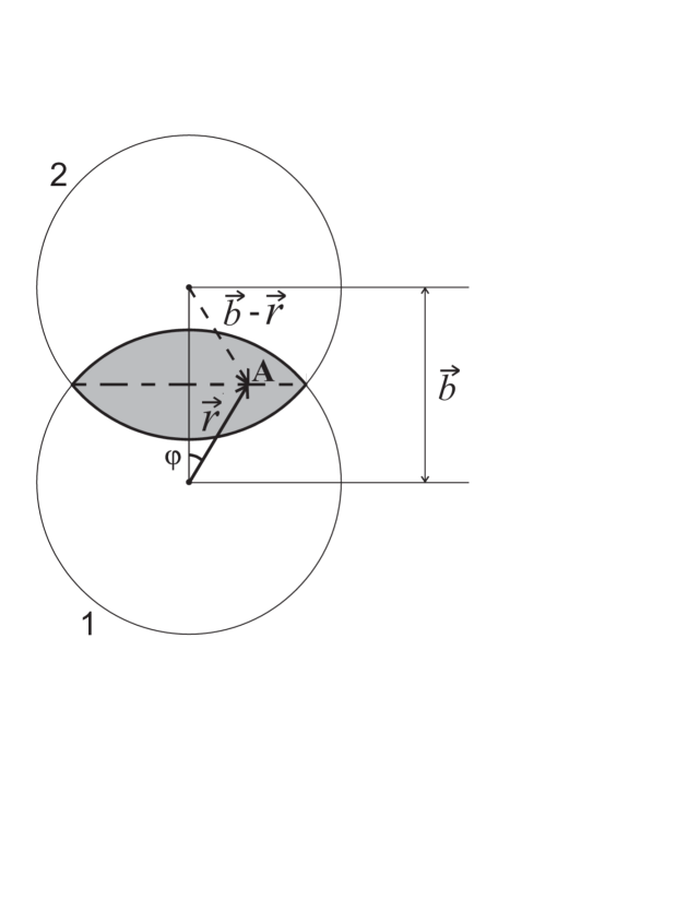
FIG. 1.: The collision geometry of nuclear collisions in the plane transverse to the beam. The parton-parton collision point is indicated by $A$ and $b$ is the impact parameter.

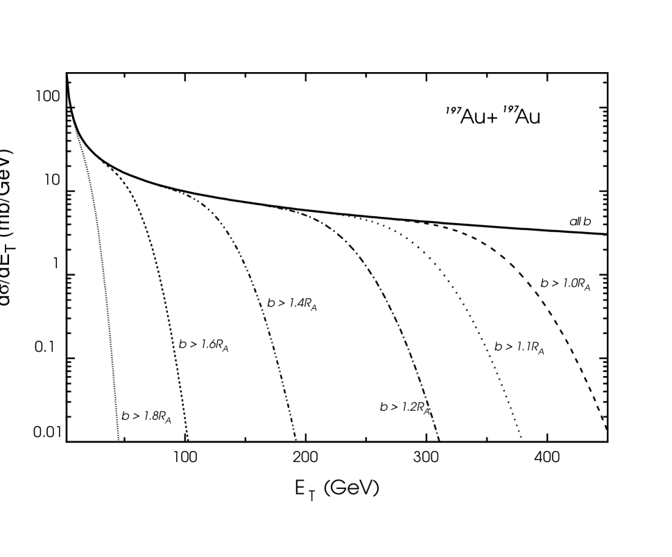
FIG. 2.: Cross section as a function of $E_{T}$, for a selection of impact parameters ranges.

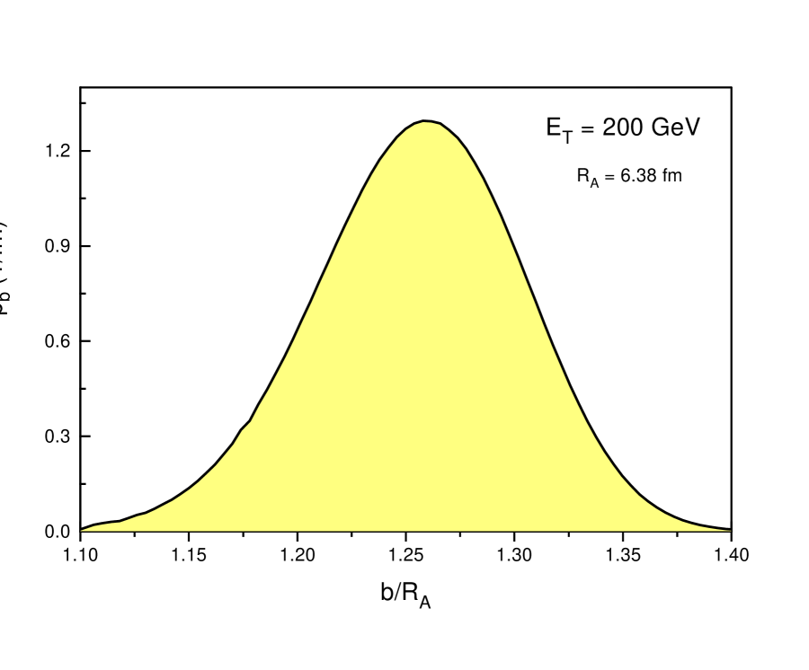
FIG. 3.: Distribution of impact parameter for events with $E_{T}=200$ GeV.

FIG. 4.: Charm production cross section as a function of $b$ for the MRS D$-^{\prime}$ parton densities, with $S=1$ (solid line) and with two nuclear shadowing parameterizations $S_{1}$ (dashes) and $S_{2}$ (dots).

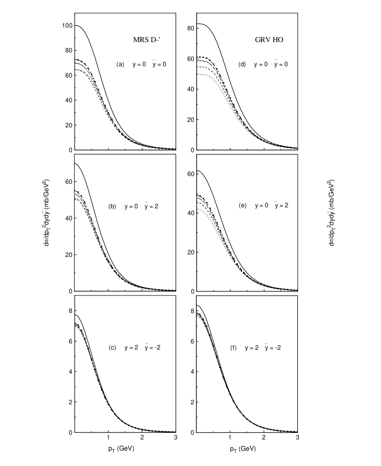
FIG. 5.: The $p_{T}$ distribution of $c\overline{c}$ pairs for the MRS D$-^{\prime}$ (a), (b) and (c) and GRV HO (d), (e) and (f) parton densities. We select events with $b>1.2R_{A}$ and 3 sets of $c$ and $\overline{c}$ quark rapidities: $y=0$, $\overline{y}=0$ in (a) and (d); $y=0$, $\overline{y}=2$ in (b) and (e); $y=2$, $\overline{y}=-2$ in (c) and (f). The solid curves are for $S=1$. The spatially independent shadowing results are given by the dashed ($S_{1}$) and dotted ($S_{2}$) curves. The effect of the spatial dependence on $S_{1}$ is also shown. The dashed curve with the filled squares shows the result with $S_{1,{\rm R}}$ and the dashed curve with the open circles gives the result with $S_{1,{\rm WS}}$. In (a), (b), (d) and (e) the $S_{1}$ and $S_{1,WS}$ curves overlap.

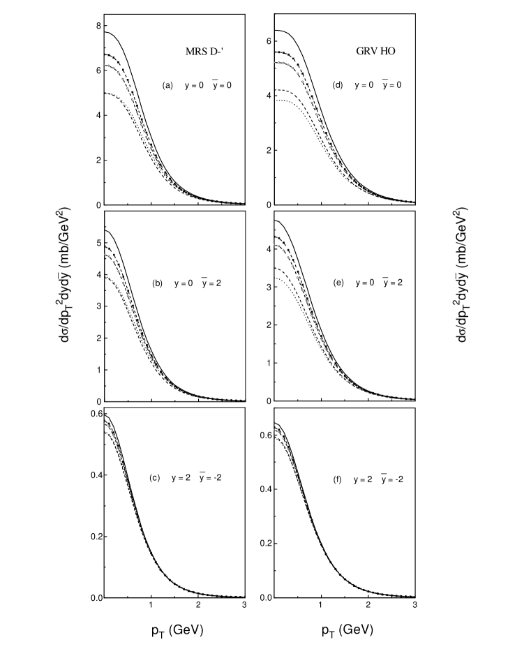
FIG. 6.: The same as in Fig. 5 but with $b>1.8R_{A}$.

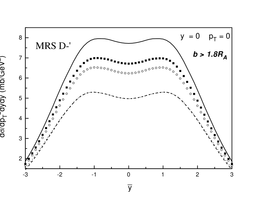
FIG. 7.: The $\overline{c}$ rapidity distribution for $p_{T}=0$ and the charm quark is produced at $y=0$. The solid curve is with $S=1$. The spatially independent shadowing results are given in the dashed and dotted curves for $S_{1}$ and $S_{2}$ respectively. The effect of the spatial dependence on $S_{1}$ is also shown. The filled squares shows the result with $S_{1,{\rm R}}$ and the open circles gives the result with $S_{1,{\rm WS}}$.

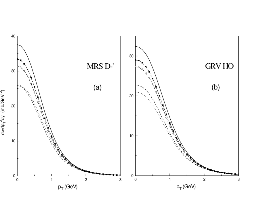
FIG. 8.: The $p_{T}$ distribution for single charm quarks with $y=0$ for MRS D$-^{\prime}$ (a) and GRV HO (b) parton densities. We have selected events with $b>1.8R_{A}$. The solid curves are with $S=1$. The spatially independent shadowing results are given in the dashed and dotted curves for $S_{1}$ and $S_{2}$ respectively. The effect of the spatial dependence on $S_{1}$ is also shown. The dashed curve with the filled squares shows the result with $S_{1,{\rm R}}$ and the dashed curve with the open circles gives the result with $S_{1,{\rm WS}}$.

REFERENCES

- [1] J.J. Aubert et al., Nucl. Phys. B293 740, (1987); M. Arneodo, Phys. Rep. 240 301, (1994).
- [2] D.M. Alde et al., Phys. Rev. Lett. 66 133, (1991).
- [3] J.A. Appel, Ann. Rev. Nucl. Part. Sci. 42 367, (1992).
- [4] L.V. Gribov, E.M. Levin, and M.G. Ryskin, Phys. Rep. 100 1, (1983).
- [5] S. Gavin, P.L. McGaughey, P.V. Ruuskanen and R. Vogt, Phys. Rev. C54 2606, (1996).
- [6] Conceptual Design for the Relativistic Heavy Ion Collider, BNL-52195, May, 1989, Brookhaven National Laboratory.
- [7] V. Emel’yanov, A. Khodinov and M. Strikhanov, Yad. Fiz. 60, 539 (1997). [Phys. of Atomic Nuclei 60 539, (1997)].
- [8] M. Greiner et al., Phys. Rev. C51 911, (1995).
- [9] R.K. Ellis, in Physics at the 100 GeV Scale, Proceedings of the 17th SLAC Summer Institute, Stanford, California, 1989, edited by E.C. Brennan (SLAC Report No. 361, Stanford, 1990).
- [10] P. Nason, S. Dawson, and R.K. Ellis, Nucl. Phys. B303 607, (1988); Nucl. Phys. B327 49, (1989).
- [11] W. Beenakker, H. Kuijf, W.L. van Neerven, and J. Smith, Phys. Rev. D40 54, (1989); W. Beenakker, W.L. van Neerven, R. Meng, G.A. Schuler, and J. Smith, Nucl. Phys. B351 507, (1991).
- [12] P.L. McGaughey et al., Int. J. Mod. Phys. A10 2999, (1995).
- [13] A.D. Martin, W.J. Stirling, and R.G. Roberts, Phys. Lett. B306 145, (1993).
- [14] M. Glück, E. Reya, and A. Vogt, Z. Phys. C53 127, (1992).
- [15] H. Plothow-Besch, Comp. Phys. Comm. 75 396, (1993).
- [16] R. Vogt, Z. Phys. C71 475, (1996).
- [17] C.W. deJager, H. deVries, and C. deVries, Atomic Data and Nuclear Data Tables 14 485, (1974).
- [18] L.V. Gribov, E.M. Levin and M.G. Ryskin, Nucl. Phys. B188 555, (1981); Zh. Eksp. Teor. Fiz. 80 2132, (1981); A.H. Mueller and J.W. Qiu, Nucl. Phys. B258 427, (1986).
- [19] M.R. Adams et al., Phys. Rev. Lett. 68 3266, (1992).
- [20] K.J. Eskola, J. Qiu, and J. Czyzewski, private communication.
- [21] K.J. Eskola, Nucl. Phys. B400 240, (1993).
- [22] D.W. Duke and J.F. Owens, Phys. Rev. D30 49, (1984).
- [23] X.-N. Wang and M. Gyulassy, Phys. Rev. D44 3501, (1995).
- [24] K.J. Eskola, K. Kajantie and J. Lindfors, Nucl. Phys. B323 37, (1989).
- [25] K.J. Eskola, Nucl. Phys. A590 383c, (1995); K.J. Eskola, K. Kajantie and P.V. Ruuskanen, Phys. Lett. B332 191, (1994).
- [26] K.J. Eskola, R. Vogt and X.-N. Wang, Int. J. Mod. Phys. A10 3087, (1995).
- [27] K.J. Eskola, Z. Phys. C51 633, (1991).
- [28] V. Emel’yanov, A. Khodinov and M. Strikhanov, Preprint MEPHI-026 (1995).
- [29] W.B. Christie, in Physics with the Collider Detectors at RHIC and the LHC, UCRL-ID-121571, edited by J. Thomas and T.J. Hallman, 1995.
- [30] R. Vogt, S.J. Brodsky and P. Hoyer, Nucl. Phys. B383 643, (1992).
- [31] Z. Lin and M. Gyulassy, Phys. Rev. Lett. 77 1222, (1996).