Kaons in dense matter, kaon production in heavy-ion collisions, and kaon condensation in neutron stars

Abstract

The recent past witnesses the growing interdependence between the physics of hadrons, the physics of relativistic heavy-ion collisions, and the physics of compact objects in astrophysics. A notable example is the kaon which plays special roles in all the three fields. In this paper, we first review the various theoretical investigations of kaon properties in nuclear medium, focusing on possible uncertainties in each model. We then present a detailed transport model study of kaon production in heavy-ion collisions at SIS energies. We shall discuss especially the elementary kaon and antikaon production cross sections in hadron-hadron interactions, that represent one of the most serious uncertainties in the transport model study of particle production in heavy-ion collisions. The main purpose of such a study is to constrain kaon in-medium properties from the heavy-ion data. This can provide useful guidances for the development of theoretical models of the kaon in medium. In the last part of the paper, we apply the kaon in-medium properties extracted from heavy-ion data to the study of neutron star properties. Based on a conventional equation of state of nuclear matter that can be considered as one of the best constrained by available experimental data on finite nuclei, we find that the maximum mass of neutron stars is about 2$M_{\odot}$, which is reduced to about 1.5$M_{\odot}$ once kaon condensation as constrained by heavy-ion data is introduced.

pacs: 25.75.Dw, 97.60.Jd, 26.60.+c, 24.10.Lx

Key words: chiral perturbation theory, pseudoscalar mesons, particle production, relativistic heavy-ion collisions, medium effects, kaon condensation, neutron stars.

I INTRODUCTION

There is currently growing interplay between physics of hadrons (especially the properties of hadrons in dense matter which might reflect spontaneous chiral symmetry breaking and its restoration), the physics of relativistic heavy-ion collisions (from which one might extract hadron properties in dense matter), and the physics of compact objects in astrophysics (which needs as inputs the information gained from the first two fields). A notable example is the kaon ($K$ and ${\bar{K}}$), which, being a Goldstone boson with strangeness, plays a special role in all the three fields mentioned.

Ever since the pioneering work of Kaplan and Nelson [1, 2] on the possibility of kaon condensation in nuclear matter, a huge amount of theoretical effort has been devoted to the study of kaon properties in dense matter, based mostly on the SU(3) chiral perturbation theory [3, 4, 5, 6, 7, 8, 9, 10, 11, 12, 13, 14, 15, 16]. Kaons, as Goldstone bosons with strangeness, play a special role in the development of hadron models. The mass of the strange quark is about 150 MeV, which is, on the one hand, considerably larger than the mass of light (up and down) quarks ($\sim 5$ MeV), but on the other hand, much smaller than that of the charmed quark ($\sim 1.5$ GeV). In the limit of vanishing quark mass the chiral symmetry is good, and systematic studies can be carried out using chiral perturbation theory for hadrons made of light quarks. Since its mass is not negligibly small as compared with the typical QCD chiral symmetry breaking scale $\Lambda_{\chi}\sim 1$ GeV, the expansion in terms of the strange quark mass is much more delicate. In spite of this, chiral perturbation calculations have been extensively and quite successfully carried out in the recent past for the study of kaon-nucleon ($KN$) and antikaon-nucleon (${\bar{K}}N$) scattering.

Part of the reason for this success, at least in free space, can be attributed to the availability of a large body of experimental data which can be used to constrain the various parameters in the chiral Lagrangian. In studying kaon properties in nuclear matter, a new scale, namely the nuclear Fermi momentum $k_{F}$, is introduced. This renders the chiral perturbation calculation in matter much more subtle than that in free space. It is very important to have experimental data available so that the predictions of chiral perturbation calculations can be tested. Kaonic atom data provide information on this, but is restricted to very low densities [17]. For the study of kaon condensation, densities much higher than that accessible by kaonic atoms are involved. This can only be obtained by analysing heavy-ion collision data on kaon spectra and flow.

Measurements of kaon spectra and flow have been systematically carried out in heavy-ion collisions at SIS (1-2 AGeV), AGS (10 AGeV), and SPS (200 AGeV) energies [18]. By comparing transport model predictions with experimental data, one can learn not only the global reaction dynamics, but more importantly, the kaon properties in dense matter. Of special interest is kaon production in heavy-ion collisions at SIS energies, as it has been shown that particle production at subthreshold energies is sensitive to its properties in dense matter [19, 20, 21]. Recently, high quality data concerning $K^{+}$ and $K^{-}$ production in heavy-ion collisions at SIS energies have been published by the KaoS collaboration at GSI [22]. The KaoS data show that the $K^{-}$ yield at 1.8 AGeV agrees roughly with the $K^{+}$ yield at 1.0 AGeV. This is a nontrivial observation. These beam energies were purposely chosen, such that the Q-values (the difference between the available center-of-mass energy and the threshold) for $NN\rightarrow NK\Lambda$ and $NN\rightarrow NNK{\bar{K}}$ are identical and both are about $-230$ MeV. Near their respective production thresholds, the cross section for the $K^{-}$ production in proton-proton interaction is one to two orders of magnitude smaller than that for $K^{+}$ production [23]. In addition, antikaons are strongly absorbed in heavy-ion collisions, which should further reduce the $K^{-}$ yield. The KaoS results of $K^{-}/K^{+}\sim 1$ indicate thus the importance of kaon medium effects which act oppositely on the $K^{+}$ and $K^{-}$ production in nuclear medium, and can thus provide useful information on kaon properties in dense matter.

Studies of neutron star properties also have a long history, both observationally and theoretically. A recent compilation by Thorsett quoted by Brown [24] shows that well-measured neutron star masses are all less than 1.5$M_{\odot}$. On the other hand, most of the theoretical calculations based on conventional nuclear equation of state (EOS) predict a maximum neutron state mass above 2$M_{\odot}$ [25, 26, 27]. The EOS can, therefore, be substantially softened without running into contradiction with observation. Various scenarios have been proposed that can lead to a soft EOS. Brown and collaborators suggested that kaon condensation might happen at a critical density of 2-4$\rho_{0}$ [28]. The existence of many $K^{-}$ mesons implies the coexistence of a large number of protons that are needed to neutralize the negative charge of $K^{-}$ mesons [29]. Based on this, Brown and Bethe also proposed the interesting possibility of the existence of a large number of low mass black holes in the galaxy [30].

In the first part of this paper, Section 2, we review various theoretical approaches for studying kaon properties in nuclear medium. We shall focus on the limitations and possible uncertainties in each approach. In the second part, Section 3, we present a detailed analysis of kaon production in heavy-ion collisions at SIS energies. We will discuss in detail the elementary kaon and antikaon production cross sections in hadron-hadron interactions, which are the major sources of uncertainties in the transport model study of particle production in heavy-ion collisions. By comparing transport model predictions with experimental data, we try to extract kaon in-medium properties at high densities. This information is very useful for the development of chiral perturbation theory for finite density. This also provides guidance for the study of kaon condensation in neutron stars, which is the focus of Section 4. We calculate neutron star masses based on the nuclear equation of state (EOS) of Furnstahl, Tang and Serot [31]. Without kaon condensation, the maximum neutron star mass is predicted to be about 2.0$M_{\odot}$, which reduces to about 1.5$M_{\odot}$ once kaon condensation is introduced. The paper ends with summary and outlook in Section 5.

II kaon in dense matter: a review

Ever since the pioneering work of Kaplan and Nelson [1] on the possibility of kaon condensation in dense nuclear matter, many works have been devoted to the study of kaon properties in nuclear matter. There are two typical approaches to this problem. One was initiated by Kaplan and Nelson, and is based on the chiral perturbation theory. The other has been pursued by Schaffer et al. and Knorren et al. based on the extension of the Walecka-type mean field model from SU(2) to SU(3). In other words, it follows the traditional meson-exchange idea for hadron interactions. This latter approach has also been developed by the Jülich group for the description of kaon-nucleon scattering in free space [32, 33]. In addition, kaon properties in dense matter have been studied using the Nambu$-$Jona-Lasinio model [8], treating the kaon as quark-antiquark excitation, and phenomenological off-shell meson-nucleon interaction [6]. Although quantitatively, the results from these different models are not completely identical, qualitatively, a consistent picture, namely in nuclear matter the kaon feels a weak repulsive potential and the antikaon feels a strong attractive potential, has emerged. In this section we will discuss mainly the results of the chiral perturbation theory and the meson-exchange model.

A Chiral perturbation theory

The interactions between pseudoscalar mesons (pion, kaon, and eta meson) and baryons (nucleon and hyperon) are described by the SU(3)${}_{L}\times$SU(3)_R nonlinear chiral Lagrangian which can be written as

$${\cal L} = {1\over 4}f^{2}{\rm Tr}\partial^{\mu}\Sigma\partial_{\mu}\Sigma^{\dagger}+{1\over 2}f^{2}\Lambda[{\rm Tr}M_{q}(\Sigma-1)+{\rm h.c.}]+{\rm Tr}{\bar{B}}(i\gamma^{\mu}\partial_{\mu}-m_{B})B$$ (1)

$$+ i{\rm Tr}{\bar{B}}\gamma^{\mu}[V_{\mu},B]+D{\rm Tr}{\bar{B}}\gamma^{\mu}\gamma^{5}\{A_{\mu},B\}+F{\rm Tr}{\bar{B}}\gamma^{\mu}\gamma^{5}[A_{\mu},B]$$ (2)

$$+ a_{1}{\rm Tr}{\bar{B}}(\xi M_{q}\xi+{\rm h.c.})B+a_{2}{\rm Tr}{\bar{B}}B(\xi M_{q}\xi+{\rm h.c.})$$ (3)

$$+ a_{3}[{\rm Tr}M_{q}\Sigma+{\rm h.c.}]{\rm Tr}{\bar{B}}B.$$ (4)

In the above, $B$ is the baryon octet with a degenerate mass $m_{B}$, and

$$\Sigma=\exp(2i\pi/f),~{}~{}{\rm and}~{}~{}\xi=\sqrt{\Sigma}=\exp(i\pi/f),$$ (5)

with $\pi$ being the pseudoscalar meson octet. The pseudoscalar meson decay constants are equal in the SU(3)_V limit and are denoted by $f=f_{\pi}\simeq 93$ MeV. The meson vector $V_{\mu}$ and axial vector $A_{\mu}$ currents are defined as

$$V_{\mu}={1\over 2}(\xi^{\dagger}\partial_{\mu}\xi+\xi\partial_{\mu}\xi^{\dagger})~{}~{}{\rm and}~{}~{}A_{\mu}={i\over 2}(\xi^{\dagger}\partial_{\mu}\xi-\xi\partial_{\mu}\xi^{\dagger}),$$ (6)

respectively. The current quark mass matrix is given by $M_{q}={\rm diag}\{m_{q},m_{q},m_{s}\}$, where we neglect the small difference between the up and down quark masses.

Expanding $\Sigma$ to order of $1/f^{2}$ and keeping explicitly only the kaon field, the first two terms in Eq. (4) can be written as

$$\partial^{\mu}\bar{K}\partial_{\mu}K-\Lambda(m_{q}+m_{s})\bar{K}K+\cdots,$$ (7)

where

$$K=\left(\matrix{K^{+}\cr K^{0}\cr}\right)~{}~{}{\rm and}~{}~{}\bar{K}=(K^{-}~{}~{}\bar{K^{0}}),$$ (8)

and the ellipsis denotes terms containing other mesons.

Keeping explicitly only the nucleon and kaon, the third and fourth terms in Eq. (4) become

$${\bar{N}}(i\gamma^{\mu}\partial_{\mu}-m_{B})N-{3i\over 8f^{2}}{\bar{N}}\gamma^{0}N\bar{K}\buildrel\leftrightarrow\over{\partial}_{t}K+\cdots,$$ (9)

where

$$N=\left(\matrix{p\cr n\cr}\right)~{}~{}{\rm and}~{}~{}\bar{N}=(\bar{p}~{}~{}\bar{n}),$$ (10)

and the ellipsis denotes terms involving other baryons and mesons.

The last three terms in Eq. (4) can be similarly worked out, and the results are

$${\rm Tr}{\bar{B}}(\xi M_{q}\xi+{\rm h.c.})B = 2m_{q}{\bar{N}}N-{{\bar{N}}N\over 2f^{2}}(m_{q}+m_{s}){\bar{K}}K+\cdots,$$ (11)

$${\rm Tr}{\bar{B}}B(\xi M_{q}\xi+{\rm h.c.}) = 2m_{s}{\bar{N}}N-{{\bar{N}}N\over f^{2}}(m_{q}+m_{s}){\bar{K}}K+\cdots,$$ (12)

$$\,[{\rm Tr}M_{q}\Sigma+{\rm h.c.}]{\rm Tr}{\bar{B}}B = 2(2m_{q}+m_{s}){\bar{N}}N-{2{\bar{N}}N\over f^{2}}(m_{q}+m_{s}){\bar{K}}K+\cdots.$$ (13)

Combining above expressions, one arrives at the following Lagrangian,

$${\cal L} = {\bar{N}}(i\gamma^{\mu}\partial_{\mu}-m_{N})N+\partial^{\mu}{\bar{K}}\partial_{\mu}K-(m_{K}^{2}-{\Sigma_{KN}\over f^{2}}{\bar{N}}N){\bar{K}}K$$ (14)

$$- {3i\over 8f^{2}}{\bar{N}}\gamma^{0}N\bar{K}\buildrel\leftrightarrow\over{\partial}_{t}K+\cdots.,$$ (15)

where the kaon mass is given by

$$m_{K}^{2}=\Lambda(m_{q}+m_{s}),$$ (16)

and the nucleon mass by

$$m_{N}=m_{B}-2[a_{1}m_{q}+a_{2}m_{s}+a_{3}(2m_{q}+m_{s})].$$ (17)

Also, the $KN$ sigma term can be expressed as

$$\Sigma_{KN} \equiv {1\over 2}(m_{q}+m_{s})\langle N|{\bar{u}}u+{\bar{s}}s|N\rangle$$ (18)

$$= -{1\over 2}(m_{q}+m_{s})(a_{1}+2a_{2}+4a_{3}).$$ (19)

We note that the last term in Eq. (15) is the usual Weinberg-Tomozawa term; it gives rise to a repulsive vector potential for $K^{+}$, and an attractive vector potential for $K^{-}$. The one that goes with the kaon mass is usually called Kaplan-Nelson term; it provides scalar attraction for both $K^{+}$ and $K^{-}$, and thus reduces their mass. The amount of scalar attraction is linearly proportional to the kaon-nucleon sigma term, $\Sigma_{KN}$. From Eq. (18) we see that $\Sigma_{KN}$ depends on three coefficients, $a_{1}m_{s}$, $a_{2}m_{s}$, and $a_{3}m_{s}$. While the first two coefficients are relatively well determined from the baryon mass splitting [4], the dominant term, $a_{3}m_{s}$, is only poorly known, mainly because of the large uncertainties in the nucleon strangeness content.

On the other hand, the kaon-nucleon sigma term can be related to pion-nucleon sigma term, $\Sigma_{\pi N}$ [34]. The latter is relatively well determined to be about 45 MeV [35],

$$\Sigma_{KN} = {(m_{q}+m_{s})\langle N|{\bar{u}}u+{\bar{s}}s|N\rangle\ \over 2m_{q}\langle N|{\bar{u}}u+{\bar{d}}d|N\rangle}\Sigma_{\pi N}$$ (20)

$$\approx {1\over 4}(1+{m_{s}\over m_{q}})(1+y)\Sigma_{\pi N},$$ (21)

where the strangeness content of nucleon is defined as

$$y={2\langle N|{\bar{s}}s|N\rangle\over\langle N|{\bar{u}}u+{\bar{d}}d|N\rangle}.$$ (22)

From the particle data book [36], we know that the average mass of the light quark is $m_{q}\approx 7.5$ MeV. There is a large uncertainty in the strange quark mass $m_{s}$ which ranges from 100 to 300 MeV [36]. There is also a large uncertainty in the nucleon strangeness content, which ranges from 0 to about 0.3 [4, 37].

In the mean-field approximation and including only the Weinberg-Tomozawa and the Kaplan-Nelson terms, the kaon dispersion relation in nuclear matter is then given by

$$\omega^{2}({\bf p},\rho_{B})=m_{K}^{2}+{\bf p}^{2}-{\Sigma_{KN}\over f^{2}}\rho_{S}+{3\over 4}{\omega\over f^{2}}\rho_{N},$$ (23)

where p is the three-momentum of the kaon. From the dispersion relation, the kaon energy in medium can be obtained, i.e.,

$$\omega_{K}=\left[m_{K}^{2}+{\bf k}^{2}-{\Sigma_{KN}\over f^{2}}\rho_{S}+\left({3\over 8}{\rho_{N}\over f^{2}}\right)^{2}\right]^{1/2}+{3\over 8}{\rho_{N}\over f^{2}},$$ (24)

and similarly for the antikaon,

$$\omega_{\bar{K}}=\left[m_{K}^{2}+{\bf k}^{2}-{\Sigma_{KN}\over f^{2}}\rho_{S}+\left({3\over 8}{\rho_{N}\over f^{2}}\right)^{2}\right]^{1/2}-{3\over 8}{\rho_{N}\over f^{2}}.$$ (25)

Note that the scalar attraction depends on nucleon scalar density $\rho_{S}$, which is model dependent [9].

There are a number of corrections to these simple mean-field results. Below we discuss some of them.

Range term: At the same order in chiral perturbation theory as the Kaplan-Nelson term is the energy-dependent range term. This has been studied in great detail in Refs. [10, 14]. It has been shown that the range term reduces the scalar attraction and can be approximately included, with $\Sigma_{KN}\approx 400$ MeV, by multiplying the Kaplan-Nelson term by a factor $1-0.37\omega_{K,{\bar{K}}}^{2}/m_{K}^{2}$ [10]. Note that in the nuclear medium, the kaon effective mass increases, while that of the antikaon decreases. Therefore, while the range term is very important for $K^{+}$, it is less so for $K^{-}$. In other words, the scalar attraction for $K^{+}$ is different from that for $K^{-}$.

Brown-Rho scaling: In the nuclear medium, the pion decay constant $f_{\pi}$ may decrease [38]. At finite density, this can be easily seen from the Gell-Mann$-$Oakes$-$Renner relation. In Ref. [34], Brown and Rho has shown that the scaling in $f_{\pi}$ is instructive in linking the chiral Lagrangian in free space to Walecka mean-field model for finite nuclei. The enhancement of low-mass dileptons in heavy-ion collisions might be considered as empirical evidence for this scaling [39, 40, 41]. Including this scaling, the vector attraction for $K^{-}$ increases significantly.

Short-range correlations: At high densities, a simple mean-field type treatment of kaon-nucleon and nucleon-nucleon interactions might be inadequate. The effects of short-range correlations in nucleon-nucleon and kaon-nucleon interactions were studied by Pandharipande, Pethick, and Thorsson [42], and were found to reduce the scalar attraction significantly. There will, however, be a tendency for the effects from scaling in $f_{\pi}$ and short range correlation to cancel each other.

$\Lambda(1405)$ and coupled-channel effects: The isospin averaged $K^{-}N$ scattering length is negative in free space [43], implying a repulsive $K^{-}$ optical potential in the simple impulse approximation. However, a systematic analysis of the kaonic atom data shows that the $K^{-}$ optical potential is deeply attractive, with a value of about 200$\pm$ 20 MeV at normal nuclear matter density [17]. Unlike the kaon which interacts with nucleons relatively weakly so that the impulse approximation is reasonable, the antikaon interacts strongly with nucleons so we do not expect the impulse approximation to be reliable. The antikaon-nucleon (${\bar{K}}N$) interaction at low-energy is strongly affected by the $\Lambda(1405)$ which is a quasi bound state of an antikaon and a nucleon in the isospin $I=0$ channel and can decay into $\Sigma\pi$ channel [13]. Thus, in principle one needs to carry out a coupled-channel calculation for ${\bar{K}}N$, $\Lambda\pi$ and $\Sigma\pi$ including the effects of $\Lambda(1405)$ in both free space and in nuclear medium [13, 44, 45]. This has been studied in detail by Weise and collaborators [15, 16]. In effective chiral Lagrangian, however, one can also introduce $\Lambda(1405)$ as a fundamental field, which is consistent with phenomenological ${\bar{K}}N$ scattering amplitudes and branching ratios [46]. Because of Pauli blocking effects on the intermediate states, the possibility of forming a bound ${\bar{K}}N$ state ($\Lambda(1405)$) decreases with increasing density, leading to a dissociation of $\Lambda(1405)$ in nuclear medium. This induces a transition of the $K^{-}$ potential from repulsion at very low densities to attraction at higher densities [13, 45]. It was shown in Refs. [10, 14], that, because of the diminishing role of $\Lambda(1405)$ in dense matter, the prediction for the kaon condensation threshold is relatively robust with respect to different treatments of $\Lambda(1405)$.

In view of large uncertainties in $\Sigma_{KN}$ and difficulties in treating systematically high-order corrections, we adopt in this paper a more phenomenological approach. We assume that the effects from the scaling in $f_{\pi}$ and short-range correlations approximately cancel each other. Furthermore, we introduce two free parameters, $a_{K}$ and $a_{\bar{K}}$, which determine the scalar attractions for $K^{+}$ and $K^{-}$. We assume that these are density independent, although in principle they should be density dependent, since the range term, the scaling in $f_{\pi}$, and the short-range corrections are all density dependent. The kaon and antikaon energy in the nuclear medium can then be written as

$$\omega_{K}=\left[m_{K}^{2}+{\bf k}^{2}-a_{K}\rho_{S}+(b_{K}\rho_{N})^{2}\right]^{1/2}+b_{K}\rho_{N},$$ (26)

$$\omega_{\bar{K}}=\left[m_{K}^{2}+{\bf k}^{2}-a_{\bar{K}}\rho_{S}+(b_{K}\rho_{N})^{2}\right]^{1/2}-b_{K}\rho_{N},$$ (27)

where $b_{K}=3/(8f_{\pi}^{2})\approx 0.333$ GeVfm³. We try to determine $a_{K}$ and $a_{\bar{K}}$ from the experimental observables in heavy-ion collisions.

Since the kaon-nucleon interaction is relatively weak as compared to other hadron-nucleon interactions, impulse approximation is considered to be reasonable for the kaon potential in nuclear matter, at least at low densities. This provides some constraint on $a_{K}$. Using $a_{K}=0.22$ GeV²fm³, we find that at normal nuclear matter density $\rho_{0}=0.16$ fm^-3, the $K^{+}$ feels a repulsive potential of about 20 MeV. This is in rough agreement with what is expected from the impulse approximation using the $KN$ scattering length in free space. Note that as $\rho$ approaches zero,

$$a_{K}\approx{0.63\Sigma_{KN}\over f_{\pi}^{2}}.$$ (28)

Therefore $a_{K}=0.22$ GeV²fm³ implies $\Sigma_{KN}\approx 400$ MeV. This is exactly the value determined in Ref. [10] by fitting the $KN$ scattering length.

Determination of the $a_{\bar{K}}$ is more delicate, as impulse approximation does not apply. The $a_{\bar{K}}$ should show stronger density dependence than $a_{K}$, as the effects of $\Lambda(1450)$ and coupled-channels are both strongly density dependent. We will try to determine this value by fitting to heavy-ion data. We find that, when using the model of Furnstahl, Tang, and Serot [31] for dense matter, $a_{\bar{K}}=0.45$ GeV²fm³ provides a good fit to the $K^{-}$ data in heavy-ion collisions at SIS energies. Since the $K^{-}$ production chiefly proceeds at the high densities ($2\rho_{0}$-$3\rho_{0}$), the value of $a_{\bar{K}}$ determined here needs not apply to lower densities, e.g., those sampled in kaonic atoms.

With these two parameters we show in Fig. 1 the effective masses of kaon and antikaon defined as their energies at zero momentum. It is seen that the kaon mass increases slightly with density, resulting from near cancellation of the attractive scalar and repulsive vector potential. The mass of the antikaon drops substantially. At normal nuclear matter density, the kaon mass increases about 4%, in rough agreement with the prediction of impulse approximation based on $KN$ scattering length. The antikaon mass drops by about 22%, which is somewhat smaller than what has been inferred from the kaonic atom data [17], namely, an attractive $K^{-}$ potential of $200\pm 20$ MeV at $\rho_{0}$.

From their in-medium dispersion relations, we can define the kaon and antikaon potential as the difference between its energies in the medium and in free space [47],

$$U_{K,{\bar{K}}}=\omega_{K,{\bar{K}}}-\omega_{0},$$ (29)

with $\omega_{0}=\sqrt{m_{K}^{2}+{\bf p}^{2}}$. Kaon and antikaon potentials at two different momenta are shown in Fig. 2. The open circle in the figure is the $K^{+}$ potential expected from the impulse approximation using the kaon-nucleon scattering length in free space [48, 49]. The solid circle is the $K^{-}$ potential extracted from the kaonic atom data [17].

B Meson-exchange model

The chiral Lagrangian as given above does not describe properly the nuclear matter properties. Therefore in most of the studies about kaon condensation in density matter, the nuclear matter properties are obtained based on some form of Walecka-type mean-field model; e.g., in this work we use the model of Ref. [31], which has imposed chiral constraints on the mean field. The question then is, as put forward in Ref. [50], whether it is possible to describe the kaon-nucleon interaction using the idea of meson-exchange. This has been addressed by Schaffer et al. [9] for symmetric nuclear matter, and by Knorren et al. [50] for more general case as encountered in neutron stars.

In the meson-exchange picture, the scalar and vector interaction between kaon and nucleon are mediated by the exchange of $\sigma$ and $\omega$ meson, respectively. Although in chiral Lagrangians one cannot attach mean fields to Goldstone bosons, in the sense of Ref. [34], one might try to describe the effects of explicit chiral symmetry breaking by a scalar field $\sigma$. The Lagrangian is,

$${\cal L}_{K}=\partial_{\mu}{\bar{K}}\partial_{\mu}K-(m_{K}^{2}-g_{\sigma K}m_{K}\sigma)K{\bar{K}}+ig_{\omega K}\omega_{0}\bar{K}\buildrel\leftrightarrow\over{\partial}_{t}K,$$ (30)

where $\sigma$ and $\omega_{0}$ are the scalar and the (time-component of) vector fields, respectively. $g_{\sigma K}$ and $g_{\omega K}$ are the coupling constants between the kaon and the scalar and the vector fields, respectively. The energies of kaon and antikaon in nuclear medium are then given by

$$\omega_{K}=\left[m_{K}^{2}+{\bf k}^{2}-g_{\sigma K}m_{K}\sigma+(g_{\omega K}\omega_{0})^{2}\right]^{1/2}+g_{\omega K}\omega_{0},$$ (31)

$$\omega_{\bar{K}}=\left[m_{K}^{2}+{\bf k}^{2}-g_{\sigma K}m_{K}\sigma+(g_{\omega K}\omega_{0})^{2}\right]^{1/2}-g_{\omega K}\omega_{0}.$$ (32)

The results in the meson-exchange picture also have model dependence. First, they depend on the strength of the scalar and vector fields, which might be constrained from the nuclear matter properties. Second, they depend on the coupling constants $g_{\sigma K}$ and $g_{\omega K}$. In the simple quark model, $g_{\omega K}/g_{\omega N}\approx 1/3$, since there is only one light quark in kaon. The relation for scalar couplings is more subtle, since there is no fundamental scalar meson; it represent correlated s-wave two-pion exchange.

By analysing kaon-nucleon scattering in the meson-exchange model, and by fitting to experimental data, one may be able to determine these coupling constants. This is the approach adopted in Refs. [32, 33] by the Jülich group. The coupling constants so determined, however, cannot be used directly in Eqs. (31) and (32), as these expressions are obtained in the simple mean-field approximation, while in Refs. [32, 33], more much complete diagram sets and infinite summation of ladder diagrams are involved. This is analogous to the case of nuclear matter saturation, namely, one cannot apply directly the coupling constants in the Bonn model to the Walecka-type mean-field model for nuclear matter saturation.

Starting from the Bonn model for nucleon-nucleon interaction, one can carry out Dirac-Brueckner-Hartree-Fock calculation to study nuclear matter properties. In the same sense, one can study kaon properties in nuclear matter starting from the Jülich kaon-nucleon (and antikaon-nucleon) interactions, by solving in-medium scattering equation (the so-called G-matrix). This kind of approach should provide a consistent way of study hadron systems containing strangeness degrees of freedom.

III kaon production in heavy-ion collisions

One of the most important ingredients in the transport model study of particle production in heavy-ion collisions is the elementary particle production cross sections in hadron-hadron interactions. At SIS energies, the colliding system consists mainly of nucleons, delta resonances, and pions. We need thus kaon and antikaon production cross sections from nucleon-nucleon ($NN$), nucleon-delta ($N\Delta$), delta-delta ($\Delta\Delta$), pion-nucleon ($\pi N$), and pion-delta ($\pi\Delta$) interactions. In addition, the antikaon can also be produced from strangeness-exchange processes such as $\pi Y\rightarrow{\bar{K}}N$. In the next two subsections, we will discuss these cross sections. Because of the lack of experimental data, especially near production threshold that are important for heavy-ion collisions at SIS energies, we have to adopt the strategy that combines the parameterization of experimental data with some theoretical investigations and reasonable assumptions and prescriptions.

A Elementary kaon production cross sections

In this subsection we discuss kaon production cross sections in pion-baryon and baryon-baryon collisions.

1 kaon production in pion-baryon interactions

Two major processes for kaon production in $\pi N$ interaction, namely, $\pi N\rightarrow\Lambda K$ and $\pi N\rightarrow\Sigma K$, have actually been measured quite extensively in the literature [23]. Cugnon and Lombard proposed the following parameterizations for experimental data in some specific channels [51],

$$\sigma_{\pi^{-}p\rightarrow\Lambda K^{0}} = \left\{\begin{array}[]{lll}9.89(\sqrt{s}-\sqrt{s_{0}})\;{\rm mb}&{\rm if}&\sqrt{s_{0}}=m_{\Lambda}+m_{K}<\sqrt{s}<1.7\;{\rm GeV}\\ {0.09\over\sqrt{s}-1.6}\;{\rm mb}&{\rm if}&\sqrt{s}>1.7\;{\rm GeV}\\ \end{array}\right.,$$ (35)

$$\sigma_{\pi^{+}p\rightarrow\Sigma^{+}K^{+}} = \left\{\begin{array}[]{lll}3.21(\sqrt{s}-\sqrt{s_{0}})\;{\rm mb}&{\rm if}&\sqrt{s_{0}}=m_{\Sigma}+m_{K}<\sqrt{s}<1.9\;{\rm GeV}\\ {0.14\over\sqrt{s}-1.7}\;{\rm mb}&{\rm if}&\sqrt{s}>1.9\;{\rm GeV}\\ \end{array}\right.,$$ (38)

$${1\over 2}\left[\sigma_{\pi^{-}p\rightarrow\Sigma^{-}K^{+}}+\sigma_{\pi^{-}p\rightarrow\Sigma^{0}K^{0}}\right]=0.25\left[1.0-0.75(\sqrt{s}-1.682)\right]\;{\rm mb}\;\sqrt{s}>1.682\;{\rm GeV}.$$ (39)

Furthermore, under some assumptions, they obtained the isospin averaged cross sections

$$\sigma_{\pi N\rightarrow\Lambda K}={1\over 2}\sigma_{\pi^{-}p\rightarrow\Lambda K^{0}},$$ (40)

$$\sigma_{\pi N\rightarrow\Sigma K}={1\over 2}\left[\sigma_{\pi^{-}p\rightarrow\Sigma^{-}K^{+}}+\sigma_{\pi^{-}p\rightarrow\Sigma^{0}K^{0}}+\sigma_{\pi^{+}p\rightarrow\Sigma^{+}K^{+}}\right].$$ (41)

These parameterizations have been used by several groups in the study of kaon production in heavy-ion collisions at 1-2 AGeV region [52].

Recently, Tsushima et al. [53] studied kaon production in $\pi N$ and $\pi\Delta$ interactions in the resonance model. The kaon is produced mainly in the s-channel processes from the decay of baryon resonances such as $N(1650)$, $N(1710)$, $N(1720)$, and $\Delta(1920)$. The $\Delta(1920)$ in their model is treated as an effective description of the contributions from six $\Delta$-resonances between 1.9 and 1.94 GeV that have decay possibilities into $\Sigma K$ final state. Overall, very good agreement with experimental data has been achieved. One of the advantages of a model calculation is that the isospin average can be done explicitly. In addition to kaon production in the $\pi N$ interaction, these authors have also calculated kaon production cross sections in $\pi\Delta$ interactions, within the same model. Generally, these cross sections are substantially smaller than those in the $\pi N$ interaction, because the branching ratios of these resonances into $\pi\Delta$ are smaller than those into $\pi N$. In Fig. 3 we show the isospin-averaged cross sections from Ref. [53], which will be used in this study. For the $\pi N$ interaction we also show those from Cugnon and Lombard [51].

In addition to processes without the pion in the final state, the kaon can also be produced together with one or more pions. At SIS energies, these processes might not be very important, since they have a higher production threshold and are thus suppressed as compared to those without pions in the final states. They, nevertheless, may not be totally negligible, and become increasingly important as beam energy increases. Here we will consider processes with one pion in the final state.

For the $\Lambda\pi K$ channel, there are three sets of data available, and they can be approximately fitted by the following expression,

$$\sigma_{\pi^{-}p\rightarrow\Lambda\pi^{0}K^{0}}\approx\sigma_{\pi^{-}p\rightarrow\Lambda\pi^{-}K^{+}}\approx\sigma_{\pi^{+}p\rightarrow\Lambda\pi^{+}K^{+}}\approx 24.0\left(1-{s_{0}\over s}\right)^{3.16}\left({s_{0}\over s}\right)^{4.24}~{}{\rm mb},$$ (42)

where $\sqrt{s}$ is the available energy and $\sqrt{s_{0}}=m_{\Lambda}+m_{\pi}+m_{K}$. The comparison of this parameterization with experimental data is shown in Fig. 4. Assuming that all the other channels have the similar cross sections, the isospin-averaged cross section is then obtained,

$$\sigma_{\pi N\rightarrow\Lambda\pi K}\approx 40.0\left(1-{s_{0}\over s}\right)^{3.16}\left({s_{0}\over s}\right)^{4.24}~{}{\rm mb}.$$ (43)

Similarly, the six sets of available experimental data for $\Sigma\pi K$ final state can be approximately fitted by the same expression

$$\sigma_{\pi^{-}p\rightarrow\Sigma^{+}\pi^{-}K^{0}}\approx\sigma_{\pi^{-}p\rightarrow\Sigma^{0}\pi^{-}K^{+}}\approx\cdot\cdot\cdot\approx 19.4\left(1-{s_{0}\over s}\right)^{3.41}\left({s_{0}\over s}\right)^{4.25}~{}{\rm mb},$$ (44)

where $\sqrt{s_{0}}=m_{\Sigma}+m_{\pi}+m_{K}$. The comparison of this parameterization with data is shown in Fig. 5. Under the same assumption that all other channels have the similar cross sections, we get the isospin-averaged cross section

$$\sigma_{\pi N\rightarrow\Sigma\pi K}\approx 84.1\left(1-{s_{0}\over s}\right)^{3.41}\left({s_{0}\over s}\right)^{4.25}~{}{\rm mb}.$$ (45)

2 kaon production in baryon-baryon collisions

The situation of experimental measurement of kaon production in nucleon-nucleon collisions is much worse than for pion-nucleon interactions. Until very recently, there are basically no data available near the threshold. The first detailed analysis of the experimental data was carried out by Randrup and Ko [54]. They proposed the following parameterizations for the available data

$$\sigma_{pp\rightarrow p\Lambda K^{+}}=0.024{p_{max}\over m_{K}}\;{\rm mb}$$ (46)

$$\sigma_{pp\rightarrow p\Sigma^{0}K^{+}}\approx\sigma_{pp\rightarrow p\Sigma^{+}K^{0}}\approx=0.012{p_{max}\over m_{K}}\;{\rm mb},$$ (47)

where $p_{max}$ is the maximum momentum of kaon given by

$$p_{max}={1\over 2\sqrt{s}}\sqrt{\left(s-(m_{N}+m_{Y}+m_{K})^{2})\right)\left(s-(m_{N}+m_{Y}-m_{K})^{2}\right)},$$ (48)

with $\sqrt{s}$ the total energy and $m_{Y}$ the mass of hyperon in the final state.

Based on experimental data and isospin analysis, Randrup and Ko also obtained the following isospin-averaged cross sections

$$\sigma_{NN\rightarrow NYK}=0.072{p_{max}\over m_{K}}\;{\rm mb},$$ (49)

where $Y$ is either lambda or sigma hyperon. Furthermore, they have analysed the experimental data for processes with one pion in the final state, and by using the detailed-balance relation, they obtained the following expressions for kaon production in $N\Delta$ and $\Delta\Delta$ collisions,

$$\sigma_{N\Delta\rightarrow NYK}=0.054{p_{max}\over m_{K}}\;{\rm mb},$$ (50)

$$\sigma_{\Delta\Delta\rightarrow NYK}=0.036{p_{max}\over m_{K}}\;{\rm mb}.$$ (51)

Thus at the same center-of-mass energy, kaon production cross section in the $N\Delta$ collision is 3/4 of that in the $NN$ collision, while that in the $\Delta\Delta$ collision is half of that in the $NN$ collision.

Later on, Schürmann and Zwermann [55] proposed another parameterization of experimental data which treated more accurately the threshold behavior by using a quartic $p_{max}$ dependence rather the linear dependence of Randrup and Ko,

$$\sigma_{pp\rightarrow K^{+}X}=0.8p_{max}^{4}\;{\rm mb}.$$ (52)

This parameterization was fitted to the inclusive $K^{+}$ production cross section in proton-proton ($pp$) collisions. But it has often been identified with the lowest threshold process $NN\rightarrow N\Lambda K^{+}$.

Recently, some of the much needed experimental data for kaon production in $pp$ collisions near threshold have become available from the COSY-11 collaboration [56, 57]. They have measured the cross section $\sigma_{pp\rightarrow p\Lambda K^{+}}$ at 2 MeV above the threshold, and obtained a cross section of about 8 nb. Based on these as well as early experimental data, Cassing et al. proposed [58] new parameterizations for exclusive kaon production cross sections in $pp$ collisions,

$$\sigma_{pp\rightarrow p\Lambda K^{+}} = 0.732\left(1-{s_{0}\over s}\right)^{1.8}\left({s_{0}\over s}\right)^{1.5}\;{\rm mb},$$ (53)

$$\sigma_{pp\rightarrow p\Sigma^{0}K^{+}} = 0.275\left(1-{s_{0}\over s}\right)^{1.98}\left({s_{0}\over s}\right)\;{\rm mb},$$ (54)

$$\sigma_{pp\rightarrow p\Sigma^{+}K^{0}} = 0.338\left(1-{s_{0}\over s}\right)^{2.25}\left({s_{0}\over s}\right)^{1.35}\;{\rm mb},$$ (55)

where $\sqrt{s_{0}}$ are corresponding threshold. The isospin factors and the scaling factor for $N\Delta$ and $\Delta\Delta$ in these new parameterization are the same as those in Randrup-Ko parameterization.

There have been also several theoretical calculations of kaon production in baryon-baryon interactions, based mostly on one-boson-exchange model [59, 60, 61, 62, 63]. We discuss here mainly the model of Ref. [61, 63], which includes one-pion and one-kaon exchanges. By adjusting two cut-off parameters $\Lambda_{\pi}$ and $\Lambda_{K}$, very good agreement with experimental data on the kaon production cross section in $NN$ interactions has been achieved. In Fig. 6, the results for $pp\rightarrow p\Lambda K^{+}$ are compared with experimental data and various parameterizations. The open circles are early data from the compilation of Baldini et al, [23], while the solid circle is the experimental data available only very recently from the COSY-11 collaboration that measured kaon production in proton-proton interactions at 2 MeV above the threshold [56]. It is seen that our model provides a good description for both the old and new data. The parameterization of Randrup and Ko [54] is shown in the figure by the dashed curve. It describes the older experimental data (open circles) reasonably well. It however significantly overestimates the newest data point at 2 MeV above the threshold (solid circle). The assumed linear dependence on $p_{max}$ (the maximum momentum of kaon) is responsible for this incorrect threshold behaviour. The dotted curve in the figure gives the recent parameterization of Cassing et al. [58], who has specifically tried to fit the newest data from the COSY-11 collaboration.

The extension of this model to kaon production in nucleon-delta ($N\Delta$) and delta-delta ($\Delta\Delta$) collisions is straightforward, except for one complication arising from the fact that in the $\Delta\pi N$ vertex energy momentum conservation allows the pion to go on-shell. A pole develops in the pion propagator at part of the kinematically allowed region of the phase space. As a result the cross section becomes singular. This kind of singularity also appears in $N\Delta\rightarrow NN\eta$ [64], $N\Delta\rightarrow NN\phi$ [65], and $\pi\rho\rightarrow\pi\rho$ [66], via pion exchange. The same kind of singularity occurs in the process $\mu^{+}\mu^{-}\rightarrow e\bar{\nu}W^{+}$, in which the $\mu$ can decay to $e\bar{\nu}\nu_{\mu}$ and the exchanged neutrino goes on-shell in the diagram, leading to a singular cross section [67].

In Ref. [63], we applied the Peierls method [68], which takes care of the finite lifetime of the incoming $\Delta$ resonance, to regulate the singularity. The singularity is removed by the delta width gained through the energy-momentum conservation relation. This width is density independent and the resulting cross section does not diverge as the density goes to zero. The Peierls method has also been used in Ref. [67] to remove the singularity associated with muon collision.

The results for isospin-averaged kaon production cross sections are shown in Fig. 7, together with those from the parameterization of Randrup and Ko [54], with the upper curves represent the $\Lambda NK$ final state, and the lower curves the $\Sigma NK$ final state. For the $NN$ interaction, the Randrup-Ko parameterization is larger than our results, since in the former only one-pion-exchange was considered which leads to a large isospin-average factor. For $N\Delta$ and $\Delta\Delta$ interactions, our results are generally larger than the Randrup-Ko parameterization, except near the threshold. To apply these cross sections in the transport model, we have parameterized our theoretical results in terms of the following expression

$$\sigma_{BB\rightarrow NYK}={a(\sqrt{s}-\sqrt{s_{0}})^{2}\over b+(\sqrt{s}-\sqrt{s_{0}})^{x}}~{}{\rm mb}.$$ (56)

The fitted parameters $a$, $b$ and $x$ for six channels are listed in Table 1. These parameterizations are shown in Fig. 7 by dashed curves, which are seen to reproduce the solid curves quite accurately.

Table 1 Fitted parameters in Eq. (56).

	$NN\rightarrow N\Lambda K$	$NN\rightarrow N\Sigma K$	$N\Delta\rightarrow N\Lambda K$	$N\Delta\rightarrow N\Sigma K$	$\Delta\Delta\rightarrow N\Lambda K$	$\Delta\Delta\rightarrow N\Sigma K$
$a$	0.0865	0.1499	0.1397	0.3221	0.0361	0.0965
$b$	0.0345	0.167	0.0152	0.107	0.0137	0.014
$x$	2.0	2.4	2.3	2.3	2.9	2.3

In addition to processes with no pions in final states, kaons can also be produced together with one or more pions in the final states. We have analysed the available experimental data, and propose the following parameterizations from processes with one and two pions in final states. For $pp\rightarrow N\Lambda\pi K$, the three sets of experimental data can be fitted by the same expression

$$\sigma_{pp\rightarrow\Lambda p\pi^{+}K^{0}}\approx\sigma_{pp\rightarrow\Lambda p\pi^{0}K^{+}}\approx\sigma_{pp\rightarrow\Lambda n\pi^{+}K^{+}}\approx{0.084(\sqrt{s}-\sqrt{s_{0}})^{2}\over 0.45+(\sqrt{s}-\sqrt{s_{0}})^{2}}\;{\rm mb}.$$ (57)

We assume that other proton-proton ($pp$) and neutron-neutron ($nn$) channels have the same cross section. The only set of data that is available for neutron-proton ($np$) channels indicates a cross section which is about half of the $pp$ one, and we assume all other $np$ channels have the same cross section as this $np$ channel. Under these assumption we get the isospin-averaged cross section

$$\sigma_{NN\rightarrow N\Lambda\pi K}\approx{0.21(\sqrt{s}-\sqrt{s_{0}})^{2}\over 0.45+(\sqrt{s}-\sqrt{s_{0}})^{2}}\;{\rm mb}.$$ (58)

The comparison of these parameterizations with experimental data is shown in Fig. 8.

For $pp\rightarrow N\Sigma\pi K$, on the average, the five sets of available data can be fitted by the following expression

$${1\over 5}\left[\sigma_{pp\rightarrow p\Sigma^{+}\pi^{0}K^{0}}+\sigma_{pp\rightarrow p\Sigma^{+}\pi^{-}K^{+}}+\cdot\cdot\cdot\right]\approx{0.04(\sqrt{s}-\sqrt{s_{0}})^{2}\over 0.75+(\sqrt{s}-\sqrt{s_{0}})^{2}}\;{\rm mb}.$$ (59)

We assume that all the other $pp$ and $nn$ channels have the similar cross sections. For $np$ channels the three sets of available experimental data can be fitted, on the average, by the following expression,

$${1\over 3}\left[\sigma_{np\rightarrow p\Sigma^{+}\pi^{-}K^{0}}+\sigma_{np\rightarrow p\Sigma^{0}\pi^{-}K^{+}}+\sigma_{np\rightarrow p\sigma^{-}\pi^{+}K^{0}}\right]\approx{0.032(\sqrt{s}-\sqrt{s_{0}})^{2}\over 1.35+(\sqrt{s}-\sqrt{s_{0}})^{2}}\;{\rm mb}.$$ (60)

We assume that all the other $np$ channels have the similar cross sections. We thus get the isospin-averaged cross section,

$$\sigma_{NN\rightarrow N\Sigma\pi K}\approx{0.16(\sqrt{s}-\sqrt{s_{0}})^{2}\over 0.75+(\sqrt{s}-\sqrt{s_{0}})^{2}}+{0.16(\sqrt{s}-\sqrt{s_{0}})^{2}\over 1.35+(\sqrt{s}-\sqrt{s_{0}})^{2}}\;{\rm mb}.$$ (61)

The comparisons of these parameterizations with experimental data are shown in Fig. 9.

Finally, we discuss cross sections with two pions in the final state. For $pp\rightarrow N\Lambda\pi\pi K$, the available three sets of experimental data can be fitted, on the average, by the following expression,

$${1\over 3}\left[\sigma_{pp\rightarrow p\Lambda\pi^{+}\pi^{0}K^{0}}+\sigma_{pp\rightarrow p\Lambda\pi^{+}\pi^{-}K^{+}}+\sigma_{pp\rightarrow p\Lambda\pi^{+}\pi^{+}K^{0}}\right]\approx{0.08(\sqrt{s}-\sqrt{s_{0}})^{2}\over 2.25+(\sqrt{s}-\sqrt{s_{0}})^{2}}\;{\rm mb}.$$ (62)

We assume that other $pp$ and $nn$ channels have the same cross section. The only set of data that is available for $np$ channels indicates a cross section which is about half of the $pp$ one, and we assume all other $np$ channels have the same cross section as this $np$ channels. Under these assumptions we get the isospin-averaged cross section

$$\sigma_{NN\rightarrow N\Lambda\pi\pi K}\approx{0.32(\sqrt{s}-\sqrt{s_{0}})^{2}\over 2.25+(\sqrt{s}-\sqrt{s_{0}})^{2}}\;{\rm mb}.$$ (63)

The comparison of these parameterizations with experimental data is shown in Fig. 10.

A similar procedure is carried out for $NN\rightarrow N\Sigma\pi\pi K$. The six sets of data for $pp$ channels can be fitted, on the average, by the following expression,

$${1\over 6}\left[\sigma_{pp\rightarrow p\Sigma^{+}\pi^{+}\pi^{-}K^{0}}+\sigma_{pp\rightarrow p\Sigma^{+}\pi^{0}\pi^{-}K^{+}}+\cdot\cdot\cdot\right]\approx{0.05(\sqrt{s}-\sqrt{s_{0}})^{2}\over 2.25+(\sqrt{s}-\sqrt{s_{0}})^{2}}\;{\rm mb}.$$ (64)

Again, the $np$ channels have a cross section which is about half of that for $pp$ channels. Under the same assumptions as before, the isospin-averaged cross section is found to be

$$\sigma_{NN\rightarrow N\Sigma\pi\pi K}\approx{0.55(\sqrt{s}-\sqrt{s_{0}})^{2}\over 2.25+(\sqrt{s}-\sqrt{s_{0}})^{2}}\;{\rm mb}.$$ (65)

The comparisons of these parameterizations with experimental data are shown in Fig. 11.

Combining our theoretical results for $pp\rightarrow NYK^{+}$ with our parameterizations for channels with one and two pions in final state, we can calculate the inclusive $K^{+}$ production cross section in $pp$ collision which is compared with experimental data in Fig. 12. In the figure, the dotted, short-dashed, and long-dashed curves are for final states with zero, one and two pions, respectively, while the solid line is the sum of the three contributions. It is seen that our results are in good agreement with the data. In the figure we also show the Schürmann-Zwermann parameterization which was originally proposed for the inclusive $K^{+}$ production cross section in $pp$ interaction.

B Elementary antikaon production cross section

Similar to the kaon, at SIS energies, the antikaon can be produced from $\pi N$, $\pi\Delta$, $NN$, $N\Delta$, and $\Delta\Delta$ interactions. It can also be produced from the strangeness-exchange processes such as $\pi Y\rightarrow{\bar{K}}N$. Although the abundance of hyperons in heavy-ion collisions at SIS energies is small, these strangeness-exchange processes are quite important, because of a large cross section.

1 antikaon production in pion-baryon collisions

The cross sections for $\pi N\rightarrow NK{\bar{K}}$ have been analysed recently by Sibirtsev et al. [69] using a boson-exchange model. The authors found that the ratios between experimental cross sections of different charge channels can be well accounted for by this model. The isospin-averaged cross section from their model is

$$\sigma_{\pi N\rightarrow NK{\bar{K}}}=3\sigma_{\pi^{-}p\rightarrow pK^{0}K^{-}},$$ (66)

with the latter taken from the parameterization of the experimental data,

$$\sigma_{\pi^{-}p\rightarrow pK^{0}K^{-}}=1.121\left(1-{s_{0}\over s}\right)^{1.86}\left({s_{0}\over s}\right)^{2}\;{\rm mb},$$ (67)

where $\sqrt{s_{0}}=m_{N}+2m_{K}$. The comparisons of this parameterization, after including correct isospin factor for different charge channels, with the experimental data are shown in Fig. 13.

There are also processes with one pion in final states. The available experimental data indicate charge independence within a factor of two, and can be parameterized by

$$\sigma_{\pi^{-}p\rightarrow p\pi^{0}K^{0}K^{-}}\approx\sigma_{\pi^{-}p\rightarrow p\pi^{-}K^{+}K^{-}}=\cdot\cdot\cdot\approx 85.0\left(1-{s_{0}\over s}\right)^{5.5}\left({s_{0}\over s}\right)^{4.8}\;{\rm mb},$$ (68)

where $\sqrt{s_{0}}=m_{N}+m_{\pi}+2m_{K}$. The comparisons of this parameterization with experimental data are shown in Fig. 14. The isospin-averaged cross section is

$$\sigma_{\pi N\rightarrow N\pi K{\bar{K}}}=510.0\left(1-{s_{0}\over s}\right)^{5.5}\left({s_{0}\over s}\right)^{4.8}\;{\rm mb}.$$ (69)

There has been no theoretical study on antikaon production in pion-delta collisions. We assume that these cross sections, after isospin averaging, are the same as those for $\pi N$ interactions at the same center-of-mass energy.

2 antikaon production cross sections in baryon-baryon collisions

Again, the situation of experimental data for antikaon production in $NN$ collisions is worse than that for $\pi N$ interactions. Zwermann and Schürmann [70] analysed the available experimental data and, under the assumption that the cross section is charge independent, proposed the following parameterization for the isospin-averaged cross section,

$$\sigma_{NN\rightarrow NNK{\bar{K}}}=0.05p_{max}\;{\rm mb},$$ (70)

where $p_{max}$ is the maximum momentum of antikaon given by

$$p_{max}={1\over 2\sqrt{s}}\sqrt{(s-4(m_{N}+m_{K})^{2})(s-4m_{N}^{2})}.$$ (71)

Recently, Sibirtsev et al. [69] analysed this process in a boson-exchange model, using as inputs the antikaon production cross sections from pion-nucleon interactions outlined above. Their results fit the experimental data for $pp\rightarrow ppK^{0}{\bar{K}}^{0}$ quite well, but seem to underestimate the data for $pp\rightarrow npK^{+}{\bar{K}}^{0}$. We use in this work the following parameterization for this process

$$\sigma_{pp\rightarrow npK^{+}{\bar{K}}^{0}}=0.19\left(1-{s_{0}\over s}\right)^{2}\left({s_{0}\over s}\right)^{0.31}\;{\rm mb}.$$ (72)

Experimental data indicate that

$$\sigma_{pp\rightarrow ppK^{0}{\bar{K}}^{0}}\approx\sigma_{np\rightarrow ppK^{0}K^{-}}\approx{1\over 4}\sigma_{pp\rightarrow npK^{+}{\bar{K}}^{0}}.$$ (73)

The comparision of these parameterization with experimental data are shown in Fig. 15. Note that at 2 MeV above the threshold, our parameterization gives a cross section of about 0.09 nb for $pp\rightarrow ppK^{0}{\bar{K}}^{0}$. This is very close to the preliminary data of about 0.1 nb from the COSY-11 collaboration for $pp\rightarrow ppK^{+}K^{-}$ [57]. Both the $K^{+}$ and $K^{-}$ data near the thresholds from the COSY-11 collaboration are indeed very helpful in constraining the inputs of and reducing the uncertainties in the transport models. With some further assumptions about the relationship between different charge channels, we obtain the following isospin-averaged cross section

$$\sigma_{NN\rightarrow NNK{\bar{K}}}={5\over 4}\sigma_{pp\rightarrow npK^{+}{\bar{K}}^{0}}.$$ (74)

The comparision of this with the parameterization of Zwermann and Schürmann is shown in Fig. 16. Apparently, the latter is much larger than ours near the production threshold. Again the linear $p_{max}$ dependence assumed in the Zwermann-Schürmann parameterization is responsible for the incorrect threshold behavior. It should be mentioned that the Zwermann-Schürmann parameterization is for the isospin-averaged cross section $\sigma_{NN\rightarrow NNK{\bar{K}}}$. In Ref. [69], it was incorrectly compared with the inclusive $K^{-}$ production cross section in $pp$ collision.

For processes with one pion in the final state, experimental data are quite scarce. We propose the following parameterization for $pp\rightarrow pn\pi^{+}K^{0}{\bar{K}}^{0}$,

$$\sigma_{pp\rightarrow pn\pi^{+}K^{0}{\bar{K}}^{0}}\approx 0.945\left(1-{s_{0}\over s}\right)^{3}\left({s_{0}\over s}\right)^{2}\;{\rm mb}.$$ (75)

The available data for other channels indicate that

$$\sigma_{pp\rightarrow pp\pi^{+}K^{0}K^{-}}\approx\sigma_{pp\rightarrow pp\pi^{0}K^{0}{\bar{K}}^{0}}\approx{1\over 2}\sigma_{pp\rightarrow pn\pi^{+}K^{0}{\bar{K}}^{0}},$$ (76)

$$\sigma_{np\rightarrow pp\pi^{-}K^{0}{\bar{K}}^{0}}\approx{1\over 5}\sigma_{pp\rightarrow pn\pi^{+}K^{0}{\bar{K}}^{0}}.$$ (77)

The comparisons of these parameterizations with experimental data are shown in Fig. 17. With some further assumption about the relationship between different charge channels, we obtain the following isospin-averaged cross section

$$\sigma_{NN\rightarrow NN\pi K{\bar{K}}}\approx 3.31\left(1-{s_{0}\over s}\right)^{3}\left({s_{0}\over s}\right)^{2}\;{\rm mb}.$$ (78)

Finally, on the average, the available experimental data for five channels with two pions in the final state can be fitted by the following expression,

$${1\over 5}\left[\sigma_{pp\rightarrow pp\pi^{+}\pi^{0}K^{0}K^{-}}+\sigma_{pp\rightarrow pn\pi^{+}\pi^{-}K^{+}K^{0}}+\cdot\cdot\cdot\right]\approx 0.316\left(1-{s_{0}\over s}\right)^{3}\left({s_{0}\over s}\right)^{2}\;{\rm mb}.$$ (79)

The comparison of this parameterization with experimental data is shown in Fig. 18. The isospin-averaged cross section, assuming that all the other channels have the same cross section, is given by

$$\sigma_{NN\rightarrow NN\pi\pi K{\bar{K}}}\approx 4.75\left(1-{s_{0}\over s}\right)^{3}\left({s_{0}\over s}\right)^{2}\;{\rm mb}.$$ (80)

Summing up the cross sections with zero, one and two pions in the final state, we obtain the inclusive $K^{-}$ production cross section in $pp$ collision, which is compared with experimental data in Fig. 19. The dotted, short-dashed, and long-dashed curves correspond to channels with zero, one and two pions, respectively. The sum of these contribution, as shown in the figure by solid curve, agrees rather well with the data.

It is also useful to compare inclusive $K^{+}$ and $K^{-}$ production cross sections in $pp$ collisions. This is done in Fig. 20. It is seen that at the same $\sqrt{s}-\sqrt{s_{0}}$ ($\sqrt{s_{0}}=m_{N}+m_{\Lambda}+m_{K}$ for $K^{+}$ case, and $\sqrt{s_{0}}=2m_{N}+2m_{K}$ for $K^{-}$ case), the $K^{+}$ production cross section is one to two orders of magnitude larger than that of $K^{-}$ in $pp$ collisions.

3 antikaon production in pion-hyperon collisions

As mentioned, in heavy-ion collisions, the antikaon can also be produced from strange-exchange processes such as $\pi\Lambda\rightarrow{\bar{K}}N$ and $\pi\Sigma\rightarrow{\bar{K}}N$. These cross sections are not known empirically, but they can be obtained from the inverse processes, which have been studied in great detail experimentally, by using the detailed balance relation. At low energies, the experimental data on ${\bar{K}}N\rightarrow\pi Y$ can be analysed in terms of the K-matrix for three coupled channels ${\bar{K}}N$, $\Lambda\pi$, and $\Sigma\pi$ [49, 71]. Based on this model, Ko obtained the cross sections for $\pi\Lambda\rightarrow{\bar{K}}N$ and $\pi\Sigma\rightarrow{\bar{K}}N$ which can be as large as a few mb [72].

In Ref. [73], Cugnon et al. proposed the following parameterizations for the experimental data,

$$\sigma_{K^{-}p\rightarrow\Lambda\pi^{0}} = \left\{\begin{array}[]{lll}50p^{2}-67p+24\;{\rm mb}&{\rm if}&0.2<p<0.9\;{\rm GeV}\\ 3p^{-2.6}\;{\rm mb}&{\rm if}&0.9<p<10\;{\rm GeV/c}\\ \end{array}\right.,$$ (83)

$$\sigma_{K^{-}p\rightarrow\Sigma^{0}\pi^{0}}=0.6p^{-1.8},$$ (84)

$$\sigma_{K^{-}n\rightarrow\Sigma^{0}\pi^{-}} = \left\{\begin{array}[]{lll}1.2p^{-1.3}\;{\rm mb}&{\rm if}&0.5<p<1\;{\rm GeV/c}\\ 1.2p^{-2.3}\;{\rm mb}&{\rm if}&1<p<6\;{\rm GeV/c}\\ \end{array}\right.,$$ (87)

where $p$ is antikaon momentum in the laboratory frame. These parameterization do not describe the resonance structure in the data very well, as will be shown in Fig. 21. We will use the following parameterizations instead,

$$\sigma_{K^{-}p\rightarrow\Lambda\pi^{0}} = \left\{\begin{array}[]{lll}1.205p^{-1.428}\;{\rm mb}&{\rm if}&p\leq 0.6\;{\rm GeV}\\ 3.5p^{0.659}\;{\rm mb}&{\rm if}&0.6<p\leq 1\;{\rm GeV/c}\\ 3.5p^{-3.97}\;{\rm mb}&{\rm if}&p>1\;{\rm GeV/c}\\ \end{array}\right.,$$ (91)

$$\sigma_{K^{-}p\rightarrow\Sigma^{0}\pi^{0}}\approx\sigma_{K^{-}n\rightarrow\Sigma^{0}\pi^{-}} = \left\{\begin{array}[]{lll}0.624p^{-1.83}\;{\rm mb}&{\rm if}&p\leq 0.345\;{\rm GeV}\\ 0.0138/((p-0.385)^{2}+0.0017)\;{\rm mb}&{\rm if}&0.345<p\leq 0.425\;{\rm GeV/c}\\ 0.7p^{-2.09}\;{\rm mb}&{\rm if}&p>0.425\;{\rm GeV/c}\\ \end{array}\right..$$ (95)

The comparisons of these parameterizations with experimental data are shown in Fig. 21. The dotted lines give the parameterizations of Cugnon et al. [73]. According to Ref. [73], the isospin-averaged cross sections for the inverse processes are then

$$\sigma_{\pi\Lambda\rightarrow{\bar{K}}N}=2\left({p_{K}\over p_{\pi}}\right)^{2}\sigma_{K^{-}p\rightarrow\Lambda\pi^{0}},$$ (96)

$$\sigma_{\pi\Sigma\rightarrow{\bar{K}}N}={2\over 3}\left({p_{K}\over p_{\pi}}\right)^{2}(\sigma_{K^{-}p\rightarrow\Sigma^{0}\pi^{0}}+\sigma_{K^{-}n\rightarrow\Sigma^{0}\pi^{-}}),$$ (97)

where $p_{K}$ and $p_{\pi}$ are, respectively, momenta of antikaon and pion in the center-of-mass frame. These cross sections are shown in Fig. 22. At low invariant energies, they are in agreement with those obtained in Ref. [72] based on the K-matrix method. The first peak in these cross sections comes from the threshold effect, while the second peak comes from the resonance structure in the $\bar{K}N\rightarrow\pi Y$ cross sections.

C Kaon and antikaon final-state interactions

Particles produced in elementary hadron-hadron interactions in heavy-ion collisions cannot escape the environment freely and be detected. Instead, they are subjected to strong final-state interactions. For the kaon, because of strangeness conservation, its scattering with nucleons at low energies is dominated by elastic and pion production processes, which do not affect its final yield but changes its momentum spectra. Kaon-nucleon scattering was been studied in detail experimentally [74]. Data were nicely summarized in Ref. [49].

The experimental data for elastic kaon-nucleon scattering can be parameterized by

$$\sigma_{KN\rightarrow KN} = \left\{\begin{array}[]{lll}10.5+19.7(\sqrt{s}-\sqrt{s_{0}})^{1.58}\;{\rm mb}&{\rm if}&\sqrt{s}-\sqrt{s_{0}}\leq 0.2\;{\rm GeV}\\ 5.76(\sqrt{s}-\sqrt{s_{0}})/(0.056+(\sqrt{s}-\sqrt{s_{0}})^{2})\;{\rm mb}&{\rm if}&\sqrt{s}-\sqrt{s_{0}}>0.2\;{\rm GeV}\end{array}\right.,$$ (100)

where $\sqrt{s_{0}}=m_{N}+m_{K}$.

Similarly, the one-pion ($KN\rightarrow KN\pi$) and two-pion production ($KN\rightarrow KN\pi\pi$) cross sections can be parameterized as

$$\sigma_{KN\rightarrow KN\pi}=1.557(1-{s_{0}\over s})^{3.28}({s_{0}\over s})^{4.35}\;{\rm b},$$ (101)

with $\sqrt{s_{0}}=m_{N}+m_{K}+m_{\pi}$, and

$$\sigma_{KN\rightarrow KN\pi\pi}=12.87(1-{s_{0}\over s})^{6.38}({s_{0}\over s})^{4.9}\;{\rm b},$$ (102)

with $\sqrt{s_{0}}=m_{N}+m_{K}+2m_{\pi}$. The comparison of these parameterizations with experimental data is shown in Fig. 23.

The final-state interaction for the antikaon is much stronger. As mentioned, antikaons can be destroyed in the strangeness-exchange processes. They also undergo elastic scattering. We parameterize the experimental data for $K^{-}p$ total, elastic, and charge-exchange cross sections,

$$\sigma_{K^{-}p\rightarrow total} = \left\{\begin{array}[]{lll}23.5p^{-1.04}\;{\rm mb}&{\rm if}&p\leq 0.35\;{\rm GeV}\\ 0.504/((p-0.39)^{2}+0.0056)\;{\rm mb}&{\rm if}&0.35<p\leq 0.46\;{\rm GeV/c}\\ 181.9(p-0.75)^{2}+34.0\;{\rm mb}&{\rm if}&0.46<p<1.05\;{\rm GeV/c}\\ 55.2p^{-1.85}\;{\rm mb}&{\rm if}&p>1.05\;{\rm GeV/c}\\ \end{array}\right.,$$ (107)

$$\sigma_{K^{-}p\rightarrow K^{-}p} = \left\{\begin{array}[]{lll}11.2p^{-0.986}\;{\rm mb}&{\rm if}&p\leq 0.7\;{\rm GeV}\\ 5.0/((p-0.95)^{2}+0.25)\;{\rm mb}&{\rm if}&p>0.7\;{\rm GeV/c}\\ \end{array}\right.,$$ (110)

$$\sigma_{K^{-}p\rightarrow{\bar{K}}^{0}n} = \left\{\begin{array}[]{lll}1.813p^{-1.14}\;{\rm mb}&{\rm if}&p\leq 0.35\;{\rm GeV}\\ 0.0192/((p-0.39)^{2}+0.0016)\;{\rm mb}&{\rm if}&0.35<p\leq 0.43\;{\rm GeV/c}\\ 15.9/((p-0.9)^{2}+2.65)\;{\rm mb}&{\rm if}&p>0.43\;{\rm GeV/c}\\ \end{array}\right..$$ (114)

where $p$ is the momentum of the antikaon in the laboratory frame. The comparisions of these parameterizations with the experimental data are shown in Fig. 24. At low momenta, our parameterizations for the total and elastic cross sections are very similar to those proposed in Ref. [49]. For the $K^{-}n$ interaction, experimental data are available only at relatively large momenta. These data indicate the following approximate relations,

$$\sigma_{K^{-}n\rightarrow total}\approx 0.8\sigma_{K^{-}p\rightarrow total},$$ (115)

$$\sigma_{K^{-}n\rightarrow K^{-}n}\approx 0.9\sigma_{K^{-}p\rightarrow K^{-}p}.$$ (116)

The comparision of these relations with the experimental data is shown in Fig. 25.

We treat the charge-exchange process $K^{-}p\leftrightarrow{\bar{K}}^{0}n$ as ‘elastic’, since we do not have explicit isospin degrees of freedom in our transport model. Under these approximations, the isospin-averaged ${\bar{K}}N$ elastic cross section is given by

$$\sigma_{{\bar{K}}N\rightarrow{\bar{K}}N}\approx 0.5(1.9\sigma_{K^{-}p\rightarrow K^{-}p}+\sigma_{K^{-}p\rightarrow{\bar{K}}^{0}n}),$$ (117)

and the antikaon absorption cross section is given by

$$\sigma_{{\bar{K}}N\rightarrow absorption}\approx 0.9\sigma_{K^{-}p\rightarrow total}-\sigma_{{\bar{K}}N\rightarrow{\bar{K}}N}.$$ (118)

Both the elastic and absorption cross sections increase rapidly with decreasing antikaon momenta. This will have strong effects on the final $K^{-}$ momentum spectra in heavy-ion collisions.

D Some Discussions

1. Inclusive versus exclusive cross sections: As mentioned, kaon (and antikaon) can be produced in final states with zero, one, and more pions. To calculate their total production probability, inclusive cross sections such as $pp\rightarrow K^{+}X$ and $pp\rightarrow K^{-}X$ should be used. On the other hand, to treat their final-state interactions and to calculate their spectra, exclusive cross sections with specific final states, such as $pp\rightarrow p\Lambda K^{+}$ and $pp\rightarrow p\Lambda\pi K^{+}$ are needed. For $NN$ collisions, we have shown that by including exclusive processes with zero, one, and two pions in the final states, the inclusive cross sections for both $K^{+}$ and $K^{-}$ production with invariant energy up to about 5 GeV can be saturated. For $\pi N$ interaction, we have included exclusive processes with zero and one pion in final states. They are expected to saturate the inclusive cross sections with invariant energy up to about 3 GeV. Thus, as far as the heavy-ion collisions at SIS energies are concerned, we have included sufficient exclusive processes for both the $NN$ and $\pi N$ interactions.

2. Total versus differential cross sections: So far we have discussed only total cross sections for kaon and antikaon production in a specific channel, which give their production probabilities. To calculate their spectra and to treat their final-state interactions, we need also to determine their momenta. We need thus also differential cross sections, such as momentum spectra and angular distributions. There are far less experimental data on differential cross sections than on total cross sections. Model calculations trying to describe both the differential and total cross sections are also far more involved [60] than the one-boson-exchange model of Ref. [61] that attempted at total cross sections only.

For two-body final states, such as $\pi N\rightarrow YK$, the magnitude of the kaon momentum in the $\pi N$ center-of-mass frame is fixed. We thus need only angular distribution to determine the direction of the momentum. In all the transport model calculations, this is assumed to be isotropic in the $\pi N$ center-of-mass frame. We will also use this assumption in this work. It is expected that, because of strong final-state interaction, the use of an anisotropic angular distribution will not have significant effects on the final kaon momentum spectra. To see more quantitatively the effects of angular distribution, we will take $\pi N\rightarrow YK$ as an example, where limited experimental data are available [75]. In Fig. 26 we show the angular distribution for $\pi^{-}p\rightarrow\Lambda K^{0}$ at $\sqrt{s}=1.742$ GeV. The open circles are experimental data, and the solid curve is our parameterization,

$${d\sigma\over d\Omega}=0.01+0.0175({\rm cos}\theta+0.93)^{2}~{}{\rm mb/sr}.$$ (119)

We neglect the beam energy dependence of the angular distribution. The results for kaon final spectra using this angular distribution will be compared with those using isotropic assumption.

For three-body final states, such as $pp\rightarrow p\Lambda K^{+}$, only the maximum momentum of the kaon is fixed by energy-momentum conservation. Usually one first determine the magnitude of the kaon momentum in the $pp$ center-of-mass frame by using some sort of momentum spectra. Randrup and Ko proposed the following momentum spectra, which has been frequently used in transport models,

$${d\sigma\over dp}\sim\left({p\over p_{max}}\right)^{2}\left(1-{p\over p_{max}}\right),$$ (120)

where $p_{max}$ is the maximum momentum of the kaon in the $NN$ center-of-mass frame. This parameterization is seen to describe the experimental data [76] quite well, as can be seen from Fig. 27, which will also be used in the present work. To see the effects of elementary kaon momentum spectra on the final kaon momentum distribution in heavy-ion collisions, we will also use a somewhat different parameterization, which also provides a reasonable description of the data,

$${d\sigma\over dp}\sim\left({p\over p_{max}}\right)^{3}\left(1-{p\over p_{max}}\right)^{2}.$$ (121)

This parameterization is also compared with the data in Fig. 27.

3. In-medium versus free-space cross sections: As cab seen from last subsections, we have parameterized all the elementary production cross sections in terms of $\sqrt{s}$ and $\sqrt{s_{0}}$, where $\sqrt{s}$ is the available energy and $\sqrt{s_{0}}$ is the threshold. In nuclear medium, kaon and antikaon masses are modified, so are their production thresholds. We will then use $\sqrt{s_{0}^{*}}$, which are calculated with effective masses, in evaluating the in-medium production cross sections. This amounts to the change of threshold, or approximately, to the change of available phase space. This kind of treatment of medium effects is certainly incomplete. In nuclear medium, not only hadron masses, but also coupling constants, cut-off parameters, and even the structure of the cross sections might change. Nevertheless, the change of the thresholds, or phase space, is the most apparent and the simplest to implement. To study other medium effects, one needs a complete theory for the elementary cross sections.

Since the $K^{+}$ mass increases and the $K^{-}$ mass decrease in nuclear medium, the $K^{+}$ production cross sections are suppressed while those of $K^{-}$ are enhanced in heavy-ion collisions, when medium effects on their masses are included. This leads to an increase of $K^{-}/K^{+}$ ratio with nuclear density, as illustrated schematically in Ref. [77]. This increase is partly responsible for the observed $K^{-}/K^{+}$ ratio by the Kaos collaboration [22]. We will come back to this point later.

In addition to the change in the production cross sections, the medium effects on kaon and antikaon also affect their momentum spectra, when they propagate in the mean-field potentials. The Hamilton equations of motion for kaon and antikaon are very similar to those for nucleons,

$${d{\bf r}\over dt}={{\bf k}\over\omega_{K,{\bar{K}}}\mp b_{k}\rho_{N}},\;\;{d{\bf k}\over dt}=-\nabla_{x}U_{K,{\bar{K}}},$$ (122)

where minus sign corresponds to kaon, and plus sign to antikaon. It is clearly that the $K^{+}$ momentum increases and that of $K^{-}$ decreases when they propagate in their respective mean field potentials. This is affect significantly their momentum spectra, and especially the momentum spectra of their ratio.

E Relativistic transport model

Heavy-ion collisions involve very complicated nonequilibrium dynamics. In order to extract useful information on, e.g., nuclear equation of state and hadronic properties in dense matter, it is necessary to use transport models. At SIS energies, both mean-field and two-body scattering play important roles in the dynamical evolution of the system and need to be included. Over more than ten years, Boltzmann-Uehling-Uhlenbeck (BUU) and similar models based on either Skyrme-type or Walecka-type effective nucleon-nucleon interactions have been developed [19, 20, 78, 79]. In this work we used the relativistic transport model (RVUU) similar to that developed in Ref. [80] and used in Refs. [81, 82]. Instead of the usual linear and non-linear $\sigma$-$\omega$ [83] as in Refs. [80, 81, 82], we base our model on an effective chiral Lagrangian recently developed by Furnstahl, Tang, and Serot [31], which will also be used in our studies of neutron star properties.

The effective chiral Lagrangian of Furnstahl, Tang and Serot is derived using the dimensional analysis, naturalness arguments, and provide a very good description of nuclear matter and finite nuclei. In the mean-field approximation, the energy density for the general case of asymmetric nuclear matter is given by

$$\varepsilon = {2\over(2\pi)^{3}}\int_{0}^{K_{F_{p}}}d{\bf k}\sqrt{{\bf k}^{2}+m_{N}^{*2}}+{2\over(2\pi)^{3}}\int_{0}^{K_{F_{n}}}d{\bf k}\sqrt{{\bf k}^{2}+m_{N}^{*2}}$$ (123)

$$+ W\rho+R{1\over 2}(\rho_{p}-\rho_{n})-{1\over 2C_{V}^{2}}W^{2}-{1\over 2C_{\rho}^{2}}R^{2}+{1\over 2C_{S}^{2}}\Phi^{2}$$ (124)

$$+ {S^{\prime 2}\over 4C_{S}^{2}}d^{2}\left\{\left(1-{\Phi\over S^{\prime}}\right)^{4/d}\left[{1\over d}{\rm ln}\left(1-{\Phi\over S^{\prime}}\right)-{1\over 4}\right]+{1\over 4}\right\}-{\xi\over 24}W^{4}-{\eta\over 2C_{V}^{2}}{\Phi\over S^{\prime}}W^{2}.$$ (125)

In the above the first line represents the ‘kinetic energy’ of nucleons, with $K_{F_{p}}$ and $K_{F_{n}}$ being proton and neutron Fermi momenta determined from their densities, $\rho_{p}$ and $\rho_{n}$. The nucleon effective mass $m_{N}^{*}$ is related to its scalar field $\Phi$ by $m_{N}^{*}=m_{N}-\Phi$. In the second line, $W$ (from $\omega$ meson exchange) and $R$ (from $\rho$ meson exchange) are the isospin-even and isospin-odd vector potentials, respectively. The latter vanishes for symmetric nuclear matter. The third line includes the self-interactions of the scalar field (proportional to the anomalous dimension $d$), the vector field (proportional to $\xi$), and the coupling between them (proportional to $\eta$). The parameters of this model are adjusted to fit the properties of nuclear matter and finite nuclei. We will use the parameter set T1 listed in table 1 of Ref. [31]. The nucleon scalar and vector potentials for symmetric nuclear matter are shown in Fig. 28 as a function of density. Note that because of self-interaction of the vector field and the coupling between the scalar and vector fields in this model, the vector potential tends to saturate at high densities. In the usual linear Walecka model and non-linear $\sigma$-$\omega$ models [83], the vector potential increases linearly with density. In Ref. [84] we have shown that the inclusion of higher-order terms for vector field is instructive in reproducing correctly both the nucleon flow and dilepton data.

From the energy density, we can derive a relativistic transport model for heavy-ion collisions. At SIS energies, the colliding system consists mainly of nucleons, delta resonances, and pions. While medium effects on pions are neglected as in most transport models, nucleons and delta resonances propagate in a common mean-field potential according to Hamilton equation of motion,

$${d{\bf x}\over dt}={{\bf p}^{*}\over E^{*}},\;\;\;{d{\bf p}\over dt}=-\nabla_{x}(E^{*}+W),$$ (126)

where $E^{*}=\sqrt{{\bf p}^{*2}+m^{*2}}$. In our transport model we have neglected the explicit isospin degrees of freedom and thus the contributions from $\rho$ meson exchange. In addition to propagations in their mean field potentials, we include typical two-body scattering processes such as $BB\leftrightarrow BB$, $NN\leftrightarrow N\Delta$ and $\Delta\leftrightarrow N\pi$. Cugnon parameterizations and proper detailed-balance prescriptions are used for describing these reactions [78].

F Proton and pion observables

To show that our transport model describes reasonably the nucleon, delta and pion dynamics, we compare our predictions for proton and pion observables with recent data from the FOPI [85] collaboration. In Fig. 29 we show proton transverse mass spectra in the mid-rapidity region in central Ni+Ni collisions at 1.06, 1.45, and 1.93 AGeV. The impact parameter $b\leq 2$ fm is chosen so that fair comparison with FOPI data [85], which has a geometry cross section of about 100 mb, can be made. It is seen that our results for 1.06 AGeV agree very well with FOPI data [85]. Our spectra can be fitted by exponential function exp$(-m_{t}/T)$. The slope parameter $T$ is found to be about 95, 115, and 140 MeV at 1.06, 1.45 and 1.93 AGeV, respectively. These are also in good agreement with what have been extracted from FOPI data [85].

In Fig. 30 we show our results for $\pi^{-}$ transverse mass spectra in the same reactions as in Fig. 29. Again, our results are in very good agreement with FOPI data for central Ni+Ni collisions at 1.06 AGeV. The slope parameters of our pion spectra, fitted from $m_{t}-m$=0.1 to 0.5 GeV, are about 70, 85, and, 95 MeV for 1.06, 1.45, and 1.93 AGeV, respectively. The difference between proton and pion slope parameters can be explained by the collective transverse flow which has stronger effects on the heavier protons than pions [86].

In Fig. 31 we compare our predictions for the proton rapidity distribution in central Ni+Ni collisions with FOPI data. Here the solid circles are experimentally measured data, while the open circles are obtained from the measured data by reflecting with respect to the mid-rapidity. As in the FOPI data, in this paper $y$ is defined as the rapidity of a particle in the nucleus-nucleus center-of-mass frame, normalized by the beam rapidity. Overall very good agreement with the data have been achieved. Similar comparisons for $\pi^{-}$ rapidity distributions are shown in Fig. 32. Again, the agreement with the data is fairly good.

G Kaon and antikaon production in heavy-ion collisions

Since the proposal of Aichelin and Ko that subthreshold $K^{+}$ yield may be sensitive to nuclear equation of state at high densities [87], many works have been done concerning the subthreshold kaon production in heavy-ion collisions using various transport models [19, 20, 81, 88, 89, 90, 91, 92, 93]. There have been also several investigations on subthreshold antikaon production [58, 72, 94, 95, 96]. In this paper, we will concentrate on comparisons with recent data from the KaoS collaboration for Ni+Ni collisions [22] using the new sets of elementary cross sections as outlined in subsections A-C. We consider two scenarios, namely, with and without kaon medium effects. As mentioned, we use $a_{K}\approx 0.22$ GeV²fm³ for $K^{+}$. For $K^{-}$, we adjust $a_{\bar{K}}$ such that we achieve a good fit to the experimental $K^{-}$ spectra. We find $a_{\bar{K}}\approx 0.45$ GeV²fm³. With this value and the nuclear scalar density from the model of Furnstahl, Tang and Serot (the magnitude of the scalar attractive depends not only on the value of $a_{K,{\bar{K}}}$ but also on $\rho_{S}$, which in turn is model dependent [9]), we find that the $K^{-}$ feels an attractive potential of about 110 MeV at normal nuclear matter density, which is somewhat smaller than that extracted from kaonic atoms [17]. The $K^{-}$ production is not, however, sensitive to the lower densities as those probed in kaonic atoms.

1 Sensitivity to differential cross sections

Before presenting our main results and comparing with experimental data, we discuss in this subsection the sensitivity of final $K^{+}$ spectra to the differential cross sections. We calculate $K^{+}$ transverse mass spectra and rapidity distribution in Ni+Ni collisions at 1.8 AGeV and b=0 fm. For the sensitivity to the angular distribution we take $\pi N\rightarrow YK$ as an example. In the first case, we assume that kaons are emitted isotropically in the $\pi N$ center-of-mass frame, while in the second case, we use the angular distribution as given by Eq. 119. The results are shown in Fig. 33. As can be seen, because of rescattering, the final kaon spectra is not very sensitive to the elementary angular distribution. For the sensitivity to the momentum spectra, we take $NN\rightarrow NYK$ as an example. In the first case we use the Randrup-Ko parameterization, Eq. 120, and in the second case we use Eq. 121. The results are shown in Fig. 34. Again, as far as the elementary momentum spectra reproduce the experimental data for pp reasonably, the resulting $K^{+}$ spectra in heavy-ion collisions are very similar.

2 $K^{+}$ and $K^{-}$ kinetic energy spectra

The results for $K^{+}$ kinetic energy spectra in Ni+Ni collisions at 0.8, 1.0 and 1.8 AGeV are shown in Figs. 35, 36, and 37, respectively. The impact range is chosen to be $b\leq 8$ fm. The solid histogram gives the results with kaon medium effects, while the dotted histogram is the results without kaon medium effects. The open circles are the experimental data from the KaoS collaboration [22]. It is seen that the results with kaon medium effects are in good agreement with the data, while those without kaon medium effects slightly overestimate the data. We note that kaon feels a small repulsive potential; thus the inclusion of the kaon medium effects reduces the kaon yield. The slopes of the kaon spectra in the two cases also differ. With a repulsive potential, kaons are accelerated during the propagation, leading to a larger slope parameter as compared to the case without kaon medium effects.

The results for the $K^{-}$ kinetic energy spectra are shown in Fig. 38 for Ni+Ni collision at 1.8 AGeV. It is seen that without medium effects, our results are about a factor 3-4 below the experimental data. With the inclusion of the medium effects which reduces the antikaon production threshold, the $K^{-}$ yield increases by about a factor of 3 and our results are in good agreement with the data. This is similar to the findings of Cassing et al. [58]. Also, with the inclusion of kaon medium effects, the slope parameter of the $K^{-}$ spectra decreases, since the propagation of antikaons in their attractive potential reduces their momenta.

As mentioned earlier, the KaoS observation that the $K^{-}$ yield at 1.8 AGeV is similar to $K^{+}$ yield at 1.0 AGeV is an indication of the kaon medium effects. This can best be seen in our results by looking at their ratio as a function of kinetic energy. This is done in Fig. 39. By doing this we can also see more clearly the effects of kaon and antikaon mean-field potentials on the shapes of their momentum spectra. It is seen that without kaon medium effects, the $K^{+}/K^{-}$ ratio decreases from about 7 at low kinetic energies to about 1 at high kinetic energies. In central collisions the ratio of their total yield is $K^{+}/K^{-}\approx 6$, which is much greater than the KaoS observation of about 1. Since the antikaon absorption cross section by nucleons increases rapidly at low momentum, low-momentum antikaons are more strongly absorbed by nucleons than high-momentum ones. This makes the $K^{+}/K^{-}$ ratio increase with decreasing kinetic energies. When medium effects are included, we find that the $K^{+}/K^{-}$ ratio is almost a constant of about 1 in the entire kinetic energy region, which is in good agreement with the experimental data from the KaoS collaboration [22], shown in the figure by open circles. The ratio between their total yields in the central collisions is $K^{+}/K^{-}\approx 1.1$, very close to the KaoS observation of about 1. As mentioned, the shapes of $K^{+}$ and $K^{-}$ spectra change in opposite ways in the presence of their mean-field potential. Kaons are ‘pushed’ to high momenta by the repulsive potential, while antikaons are ‘pulled’ to low momenta. If there were no antikaon absorption, or if the absorption cross section were independent of antikaon momentum, the $K^{+}/K^{-}$ would increase with kinetic energy because of propagation in the mean-field potential. A ‘flat’ $K^{+}/K^{-}$ spectra is thus highly nontrivial, which must be result from the combined effects of mean-field and energy-dependent antikaon absorption. An accurate experimental measurement of this ratio can thus be very useful in determining whether there are medium effects or not on kaons in nuclear matter.

3 $K^{+}$ and $K^{-}$ transverse mass spectra and rapidity distributions

In Figs. 40 and 41 we show the $K^{+}$ transverse mass spectra at mid-rapidity in central Ni+Ni collisions at 1.0 and 1.93 AGeV, respectively. The impact parameter range is chosen to be $b\leq 4$ fm, comparable to the centrality selection of the FOPI collaboration’s measurement of kaon production in Ni+Ni collisions. At 1.0 AGeV, the slope parameter of the $K^{+}$ spectrum is about 60 MeV when kaon medium effects are neglected. This increases to about 70 MeV when kaon medium effects are included. At 1.93 AGeV, the slope parameters are 95 and 110 MeV, respectively, without and with kaon medium effects. Similarly, the $K^{-}$ transverse mass spectra in central Ni+Ni collisions at 1.8 AGeV are shown in Fig. 42. The difference between the scenarios with and without kaon medium effects is shown to be most pronounced at low transverse mass.

In Fig. 43, we show the $K^{+}$ rapidity distribution in central Ni+Ni collisions at 1.0 AGeV. The solid and dashed curves are obtained with and without kaon medium effects. The most significant difference between the two cases is seen around the mid-rapidities. The full width at half maximum (FWMH) is about 1.4 in the case without kaon medium effects. This increases to about 1.8 when kaon medium effects are included. The results for the $K^{+}$ rapidity spectra in Ni+Ni collisions at 1.93 AGeV are shown in Fig. 44. Here our results are compared with experimental data from the FOPI and KaoS collaborations [97]. The FOPI measured data are shown in the figure by solid circles, while the open circles are obtained by reflecting with respect to mid-rapidity. The KaoS data point, shown by solid square, is obtained by multiplying the original KaoS data measured at 1.8 AGeV by a factor of 1.45 as in Ref. [97] to take account the beam energy dependence. The agreement with the data is better when kaon medium effects are included. In this case, while the total $K^{+}$ yield agrees with the data, our rapidity distribution is somewhat broader than what the data indicate.

We show in Fig. 45 the $K^{-}$ rapidity distribution in central Ni+Ni collisions at 1.8 AGeV. The difference between the scenarios with and without kaon medium effects is most visible near mid-rapidity. In Fig. 46 we show the ratio of the $K^{+}/K^{-}$ as a function of normalized rapity $y$. As in Fig. 39, the $K^{+}$ is for beam energy of 1.0 AGeV, and the $K^{-}$ is for beam energy of 1.8 AGeV. Without kaon medium effects, we find that the ratio decreases from about 6.5 around the mid-rapidity to about 5 around the target and projectile rapidities. When kaon medium effects are included, the trend is just the opposite: the ratio increases from about 0.9 around mid-rapidity to about 2 at target and projectile rapidities. Experimental information on the rapidity dependence of the $K^{+}/K^{-}$ ratio should be very useful in distinguishing the two scenarios.

4 $K^{+}$ excitation functions

Finally, we show in Fig. 47 the beam energy dependence of $K^{+}$ yield in central Ni+Ni collisions. What is shown in the figure is the ratio between $K^{+}$ yield and participant nucleon number $A_{part}$. Our results, shown by open squares connected by solid lines, are obtained with kaon medium effects included. The data from the FOPI and KaoS collaborations are shown by solid and open circles, respectively [97, 98]. For comparison, we also plot in the figure the beam energy dependence of $\pi^{+}/A_{part}$ ratio. From 0.8 AGeV to 1.93 AGeV, the pion yield increases by about a factor of two and half, indicating an almost linear dependence on $E_{beam}$. This is in agreement with experimental observations. The $K^{+}$ yield, on the other hand, increases by about two orders of magnitude. Its beam energy dependence is about $E_{beam}^{5.3}$. The difference between the beam energy dependence of pion and kaon yield reflects the fact that at these energies kaon production is ‘subthreshold’ or ’near-threshold’, while pion production is well above the threshold.

IV kaon condensation in neutron stars

As mentioned, the medium modification of kaon properties affects not only kaon observables in heavy-ion collisions, it also bears important consequences in the structure and evolution of compact objects in astrophysics, especially the maximum mass of neutron stars. There have been many studies on this subject [5, 7, 29, 50, 99, 100]. In this paper, we emphasize the constraints on kaon in-medium properties from heavy-ion data as discussed in the last section. We shall concentrate on cold, neutrino-free neutron stars which are in chemical equilibrium under $\beta$ decay processes. We will consider two scenarios: one excludes kaons and the other includes them. In the first case, we need to find the ground state for a system of nucleons, electrons and muons in chemical equilibrium, while in the second scenario, we try to find the ground state of a system of nucleons, electrons, muons and kaons in chemical equilibrium. The ground state energy density and pressure are then used in the Tolman-Oppenheimer-Volkov (TOV) equation to study neutron star properties [29].

In the absence of kaons, the chemical equilibrium conditions require that the chemical potentials should satisfy

$$\mu=\mu_{n}-\mu_{p}=\mu_{e}=\mu_{\mu},$$ (127)

and in the presence of kaons,

$$\mu=\mu_{n}-\mu_{p}=\mu_{e}=\mu_{\mu}=\mu_{K}.$$ (128)

In both cases $\mu$ is the overall charge chemical potential. The local charge neutrality can be imposed by minimizing the thermodynamical potential

$$\Omega=\varepsilon_{N}+\varepsilon_{K}+\varepsilon_{L}-\mu(\rho_{p}-\rho_{K}-\rho_{e}-\rho_{\mu}).$$ (129)

For the energy density of nucleons we use the results of Furnstahl, Tang, and Serot, as given in Eq. (123). The energy density of leptons is given by

$$\varepsilon_{L}=\varepsilon_{e}+\eta(\mu-m_{\mu})\varepsilon_{\mu},$$ (130)

where $\eta$ is the Heaviside function ($\eta(x)=1$ if $x>0$ and $\eta(x)=0$ if $x<0$). The electron and muon energy densities are, respectively,

$$\varepsilon_{e}={\mu^{4}\over 4\pi^{2}},$$ (131)

and

$$\varepsilon_{\mu}={m_{\mu}^{4}\over 8\pi^{2}}\left[t(1+2t^{2})\sqrt{1+t^{2}}-{\rm ln}(t+\sqrt{1+t^{2}})\right],$$ (132)

where $t={K_{F_{\mu}}\over m_{\mu}}$, and $K_{F_{\mu}}^{2}=\mu^{2}-m_{\mu}^{2}$. The energy density of kaons, according to Ref. [29], is

$$\varepsilon_{K} = -f^{2}{\mu^{2}\over 2}{\rm sin}^{2}\theta+2m^{2}_{K}f^{2}{\rm sin}^{2}{\theta\over 2}+\mu x\rho$$ (133)

$$- \mu(1+x)\rho{\rm sin}^{2}{\theta\over 2}-2f^{2}a_{\bar{K}}\rho{\rm sin}^{2}{\theta\over 2},$$ (134)

where $f$ is the pion decay constant, $x=\rho_{p}/\rho$ is proton fraction, and the chiral angle $\theta$ is defined in terms of kaon amplitude $v_{K}$,

$$\theta={\sqrt{2}v_{K}\over f}.$$ (135)

The energy density $\varepsilon$ of the ground state of the system is obtained by extremizing $\Omega$ with respect to $x$, $\mu$, and $\theta$. The pressure of the system is then obtained from the energy density

$$P=\rho\left({\partial(\varepsilon/\rho)\over\partial\rho}\right).$$ (136)

The energy density $\varepsilon$ and pressure $P$ are then used in the TOV equation to obtain the properties of neutron stars,

$${dM\over dr} = 4\pi r^{2}\varepsilon$$ (137)

$${dP\over dr} = -{G[\varepsilon+P][1+4\pi r^{3}P]\over r(r-2GM)}.$$ (138)

In Fig. 48 we show the electron chemical potential as a function of nucleon density. In the case without kaons, the electron chemical potential continues to increase with nucleon density. When kaons are included, the electron chemical potential first increases up to about three times normal nuclear matter density $\rho_{0}$. Afterwards it starts to decrease because of the onset of the kaon condensation. Thus based on the kaon in-medium properties as constrained by heavy-ion data and nuclear equation of state from the model of Furnstahl, Tang and Serot, we find that the critical density for kaon condensation to be about 3$\rho_{0}$.

In Fig. 49, we show the proton fraction $x$ and rotation angle $\theta$ as a function of nucleon density. The solid and dotted curves are obtained with and without kaons. The proton fraction increases rapidly to become almost as large as the neutron fraction, after kaon condensation sets in. This reduces the asymmetry parameter, and hence the symmetry energy, of the system. The rotation angle, or the condensate amplitude, rises rapidly near the threshold, and then slowly increases to about 60⁰.

In Figs. 50 and 51 we show the energy density and pressure of system as a function of nucleon density, for both cases with and with kaons. For densities lower than 0.08 fm^-3 we use the empirical equation of state as in Ref. [29]. The match between this and the equation of state of Furnstahl et al. produces the small dip near 0.5$\rho_{0}$. Both the energy density and pressure are seen to be lowered once kaon condensation sets in. The effect is particularly strong in the pressure. Since the properties of neutron stars also depend sensitively on the ratio $P/\varepsilon$, we show in Fig. 52 the pressure as a function of energy density. The softening of the equation of state by kaon condensation is appreciable.

The results for neutron star mass as a function of central density $\rho_{cent}$ are shown in Fig. 53. It is seen that, without kaons, the maximum neutron star mass in this model is about 2$M_{\odot}$. Similar conclusions, with neutron star mass in the range of 2.1-2.3$M_{\odot}$, have been obtained in Ref. [25, 27] based on the nuclear equation of state from the Dirac-Brueckner-Hartree-Fock approach. When kaons are included, the maximum mass of neutron stars is about 1.5$M_{\odot}$. The dependence of neutron star mass on radius is shown in Fig. 54. It is seen that with kaon condensation, the radius of maximum mass neutron star increases.

V summary and outlook

In summary, we studied $K^{+}$ and $K^{-}$ production in Ni+Ni collisions at 1-2 AGeV, based on the relativistic transport model including the strangeness degrees of freedom. We found that the recent experimental data from the KaoS collaboration are consistent with the predictions of the chiral perturbation theory that the $K^{+}$ feels a weak repulsive potential and $K^{-}$ feels a strong attractive potential in nuclear medium. Using the kaon in-medium properties constrained by the heavy-ion data, we have studied neutron star properties with and without kaon condensation. The maximum mass of neutron stars is found to be about 2.0$M_{\odot}$ based on conventional nuclear equations of state obtained from the effective Lagrangian of Furnstahl et al.. This can be reduced to about 1.5$M_{\odot}$, once kaon condensation is introduced. We have emphasized the growing interdependence between hadron physics, relativistic heavy-ion physics and the physics of compact stars in astrophysics.

The recent experimental data from the COSY-11 collaboration [56, 57] on near threshold kaon and antikaon production cross section in proton-proton collisions provide much needed information for the parameterizations of elementary cross sections. It is realized that both the Randrup-Ko parameterization for $K^{+}$ production cross section and Schürmann-Zwermann parameterization for the $K^{-}$ production cross section overestimate the data near threshold by a large factor. Use of the new parameterizations that incorporate the latest COSY-11 data reduces the contributions to $K^{+}$ and $K^{-}$ yields in heavy-ion collisions from baryon-baryon interactions [58, 101]. As a result, contributions from pion-baryon and pion-hyperon interactions, that were previously found to be less important than those from baryon-baryon interaction, turn out to be important, and in some cases even become dominant.

Our knowledge on elementary cross sections has been improved over the last a few years, mainly because of the new experimental data near the threshold, and also because of the development in the theoretical study of the elementary cross sections. Nevertheless, to extract kaon medium effects from their yields in heavy-ion collisions is still a delicate task. On the other hand, the ratio, $K^{+}/K^{-}$, and especially the shapes of its transverse mass spectra and rapidity distribution, is less sensitive to the elementary cross sections, and should be able to provide more definite information about kaon in-medium properties. Also, the collective flow signals of $K^{+}$ and $K^{-}$ [102, 103, 104] in heavy-ion collisions are very useful probes of kaon medium effects.

We are grateful to C.M. Ko, T.T.S. Kuo, M. Prakash, and M. Rho for useful discussions. We thank N. Herrmann and P. Senger for sending us their data files and for useful communications. We also thank W. Weise for a careful reading of the manuscript and for critical comments. This work is supported in part by the Department of Energy under Grant No. DE-FG02-88ER40388.

FIG. 1.: Effective mass of kaon and antikaon in nuclear medium.

FIG. 2.: Kaon and antikaon potential in nuclear medium at two different momenta. The open circle in the figure is the $K^{+}$ potential expected from the impulse approximation using the kaon-nucleon scattering length in free space [48, 49]. The solid circle is the $K^{-}$ potential extracted from the kaonic atom data [17].

FIG. 3.: Isospin-averaged cross sections $\sigma_{\pi N\rightarrow YK}$. Solid and dotted lines are from Refs. [53] and [51], respectively.

FIG. 4.: Kaon production cross sections $\sigma_{\pi N\rightarrow\Lambda\pi K}$. Open circles are experimental data, and the lines are parameterizations.

FIG. 5.: Same as Fig. 4, for $\sigma_{\pi N\rightarrow\Sigma\pi K}$.

FIG. 6.: Kaon production cross section $\sigma_{pp\rightarrow p\Lambda K^{+}}$. The solid curve is the results of boson-exchange model of Ref. [61]. The dashed and dotted curves are the parameterizations of Randrup and Ko [54] and Cassing et al. [58], respectively. The open circles are experimental data from Ref. [23], while the solid circle is from Ref. [56].

FIG. 7.: Isospin-averaged kaon production cross sections $\sigma_{BB\rightarrow NYK}$. The solid lines are the results of boson-exchange model of Refs. [61, 63]. The dotted lines are the parameterizations of Randrup and Ko [54]. The dashed curves are the parameterizations Eq. (56).

FIG. 8.: Kaon production cross sections $\sigma_{NN\rightarrow N\Lambda\pi K}$. The open circles are the experimental data from Ref. [23], and the lines are parameterizations.

FIG. 9.: Same as Fig. 8, for $\sigma_{NN\rightarrow N\Sigma\pi K}$.

FIG. 10.: Same as Fig. 8, for $\sigma_{NN\rightarrow N\Lambda\pi\pi K}$.

FIG. 11.: Same as Fig. 8, for $\sigma_{NN\rightarrow N\Sigma\pi\pi K}$.

FIG. 12.: Inclusive $K^{+}$ production cross section in $pp$ collisions. The solid curve is the sum of $pp\rightarrow NYK^{+},~{}NY\pi K^{+},$ and $NY\pi\pi K^{+}$.

FIG. 13.: Antikaon production cross sections $\sigma_{\pi N\rightarrow NK{\bar{K}}}$. The open circles are experimental data from Ref. [23], and the lines are the parameterizations of Sibirtsev et al. [69].

FIG. 14.: Antikaon production cross section $\sigma_{\pi N\rightarrow N\pi K{\bar{K}}}$. The open circles are experimental data from Ref. [23], and the lines are the parameterizations.

FIG. 15.: Antikaon production cross section $\sigma_{NN\rightarrow NNK\bar{K}}$. The open circles are experimental data from Ref. [23], and the curves are our parameterizations.

FIG. 16.: Isospin-averaged antikaon production cross section $\sigma_{NN\rightarrow NNK\bar{K}}$. The solid line is from this work, and the dotted line is the parameterization of Zwermann and Schürmann [70].

FIG. 17.: Same as Fig. 15, for $\sigma_{NN\rightarrow NN\pi K\bar{K}}$.

FIG. 18.: Same as Fig. 15, for $\sigma_{NN\rightarrow NN\pi\pi K\bar{K}}$.

FIG. 19.: Inclusive $K^{-}$ production cross section in $pp$ collisions. The solid curve is the sum of $pp\rightarrow ppK^{+}K^{-},~{}NN\pi KK^{+},$ and $NN\pi\pi KK^{-}$.

FIG. 20.: Comparison of inclusive $K^{+}$ and $K^{-}$ production cross sections in $pp$ collisions.

FIG. 21.: Cross sections $\sigma_{K^{-}N\rightarrow Y\pi}$. The open circles are experimental data from Ref. [23]. The solid lines are the parameterizations in this work, and the dotted lines are the parameterizations of Cugnon et al. [73].

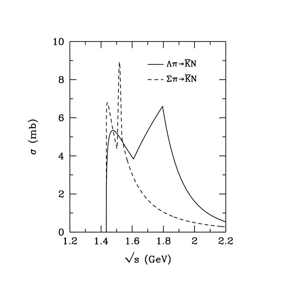
FIG. 22.: Cross sections $\sigma_{\pi Y\rightarrow{\bar{K}}N}$.

FIG. 23.: $KN$ elastic, one-pion production, and two-pion production cross sections. The symbols are experimental data from Ref. [74], and the curves are parameterizations.

FIG. 24.: $K^{-}p$ total, elastic, and charge-exchange cross sections. The symbols are experimental data from Ref. [23], and the curves are parameterizations.

FIG. 25.: Same as Fig. 24, for $K^{-}n$ total and elastic cross sections.

FIG. 26.: Angular distribution in $\pi^{-}p\rightarrow\Lambda K^{0}$ at $\sqrt{s}=1.742$ GeV. The experimental data are taken from Ref. [75], while the solid curve is our parameterization.

FIG. 27.: Kaon momentum spectra in $pp$ collisions at $\sqrt{s}=2.88$ and 2.99 GeV. The experimental data are taken from Ref. [76], while the the curves are parameterizations.

FIG. 28.: Nucleon scalar and vector potentials from the effective chiral Lagrangian of Furnstahl, Tang and Serot [31].

FIG. 29.: Proton transverse mass spectra in central Ni+Ni collisions. The open circles are experimental data from Ref. [85].

FIG. 30.: Same as Fig. 29, for $\pi^{-}$.

FIG. 31.: Proton rapidity distribution in central Ni+Ni collisions. The solid circles are experimental data from Ref. [85], the open circles are reflected with respect to mid-rapidity.

FIG. 32.: Same as Fig. 31, for $\pi^{-}$.

FIG. 33.: $K^{+}$ tranverse mass spectra and rapidity distribution in Ni+Ni collisions at 1.8 AGeV and 0 fm. The solid and dotted lines are the results with isotropic and anisotropic angular distributions, respectively.

FIG. 34.: $K^{+}$ tranverse mass spectra and rapidity distribution in Ni+Ni collisions at 1.8 AGeV and 0 fm. The solid and dotted lines are the results using Eq. (120) and Eq. (121) as momentum spectra, respectively.

FIG. 35.: $K^{+}$ kinetic energy spectra in Ni+Ni collisions at 0.8 AGeV. The solid and dotted histograms are the results with and without kaon medium effects, respectively. The open circles are experimental data from Ref. [22].

FIG. 36.: Same as Fig. 35, for Ni+Ni at 1.0 AGeV.

FIG. 37.: Same as Fig. 35, for Ni+Ni at 1.8 AGeV.

FIG. 38.: Same as Fig. 35, for $K^{-}$ spectra in Ni+Ni at 1.8 AGeV.

FIG. 39.: kinetic energy spectra of $K^{+}/K^{-}$ in Ni+Ni collisions at 1.0 AGeV ($K^{+}$) and 1.8 AGeV ($K^{-}$). The solid and dotted histograms are the results with and without kaon medium effects, respectively. The circles are the experimental data from the KaoS collaboration [22].

FIG. 40.: $K^{+}$ transverse mass spectra in central Ni+Ni collisions at 1.0 AGeV. The solid and dotted histograms are the results with and without kaon medium effects, respectively.

FIG. 41.: Same as Fig. 40, for central Ni+Ni collisions at 1.93 AGeV.

FIG. 42.: Same as Fig. 40, for $K^{-}$ in central Ni+Ni collisions at 1.8 AGeV.

FIG. 43.: $K^{+}$ rapidity distribution in central Ni+Ni collisions at 1.0 AGeV. The solid and dotted curves are the results with and without kaon medium effects, respectively.

FIG. 44.: Same as Fig. 43, for central Ni+Ni collisions at 1.93 AGeV.

FIG. 45.: Same as Fig. 43, for $K^{-}$ in central Ni+Ni collisions at 1.8 AGeV.

FIG. 46.: Rapidity distribution of $K^{+}/K^{-}$ in Ni+Ni collisions at 1.0 ($K^{+}$) and 1.8 ($K^{-}$) AGeV. The solid and dotted curves are the results with and without kaon medium effects, respectively.

FIG. 47.: Excitation function of $K^{+}/A_{part}$ and $\pi^{+}/A_{part}$ in central Ni+Ni collisions. The experimental data are from Ref. [97]

FIG. 48.: Electron chemical potential as a function of nucleon density. The solid and dotted curves are obtained with and without kaons.

FIG. 49.: Proton fraction and chiral rotation angle as a function of nucleon density. The solid and dotted curves are obtained with and without kaons.

FIG. 50.: Energy density as a function of nucleon density. The solid and dotted curves are obtained with and without kaons.

FIG. 51.: Pressure as a function of nucleon density. The solid and dotted curves are obtained with and without kaons.

FIG. 52.: Pressure as a function of energy density. The solid and dotted curves are obtained with and without kaons.

FIG. 53.: neutron star mass as a function of central density. The solid and dotted curves are obtained with and without kaons.

FIG. 54.: neutron star mass as a function of radius. The solid and dotted curves are obtained with and without kaons.

REFERENCES

- [1] D.B. Kaplan and A.E. Nelson, Phys. Lett. B175 (1986)57.
- [2] A.E. Nelson and D.B. Kaplan, Phys. Lett. B192 (1987) 193.
- [3] G.E. Brown, K. Kubodera, and M. Rho, Phys. Lett. 192B (1987) 272.
- [4] H.D. Politzer and M.B. Wise, Phys. Lett. 273B (1991) 156.
- [5] T. Muto and T. Tatsumi, Phys. Lett. 283B (1992) 165.
- [6] H. Yabu, S. Nakamura, F. Myhrer, and K. Kubodera, Phys. Lett. 315B (1993) 17.
- [7] G.E. Brown, C.-H. Lee, M. Rho, and V. Thorsson, Nucl. Phys. A567 (1994) 937.
- [8] M. Lutz, A. Steiner, and W. Weise, Nucl. Phys. A574 (1994) 755.
- [9] J. Schaffner, A. Gal, I.N. Mishistin, H. Stöcker, and W. Greiner, Phys. Lett. B334 (1994) 268.
- [10] C.-H. Lee, G.E. Brown, D.P. Min, and M. Rho, Nucl. Phys. A585 (1995) 401.
- [11] N. Kaiser, P.B. Siegel, and W. Weise, Nucl. Phys. 594 (1995) 325.
- [12] N. Kaiser, T. Waas, and W. Weise, Phys. Lett. B365 (1996) 12.
- [13] T. Waas, N. Kaiser, and W. Weise, Phys. Lett. B379 (1996).
- [14] C.-H. Lee, Phys. Rep 275 (1996) 255.
- [15] N. Kaiser, T. Waas, and W. Weise, Nucl. Phys. A612 (1997) 297.
- [16] T. Waas, M. Rho, and W. Weise, Nucl. Phys. A617 (1997) 449.
- [17] E. Friedman, A. Gal, and C. J. Batty, Nucl. Phys. A579 (1994) 518.
- [18] See e.g., QM’95, Nucl. Phys. A590 (1995); QM’96, Nucl. Phys. A610 (1996).
- [19] W. Cassing, V. Metag, U. Mosel, K. Niita, Phys. Rep. 188 (1990) 363.
- [20] C.M. Ko and G.Q. Li, J. Phys. G 22 (1996) 1673.
- [21] C.M. Ko, V. Koch, and G.Q. Li, Ann. Rev. Nucl. Part. Sci. 1997, to be published.
-
[22]
R. Barth and the KaoS Collaboration, Phys.
Rev. Lett., 78 (1997) 4027;
P. Senger for the KaoS collaboration, Heavy Ion Physics, 4, 317 (1996);
P. Senger for the KaoS collaboration, Acta Physica Polonica, B27, 2993 (1996). - [23] A. Baldini et al., Total cross sections of high energy particles, (Springer-Verlag, Heidelberg, 1988).
- [24] G. E. Brown, Proc. Royal Dutch Academy Colloquium ‘Pulsar Timing, General Relativity and the Internal Structure of Neutron Stars’, to be published
- [25] L. Engvik, E. Osnes, M. Hjorth-Jensen, G. Bao, and E. Ostgaard, Astrophy. Jour. 469 (1996) 794.
- [26] H. Müller and B.D. Serot, Nucl. Phys. A606 (1996) 508.
- [27] C.-H. Lee, T.T.S. Kuo, G.Q. Li, and G.E. Brown, to be published.
- [28] G.E. Brown, K. Kubodera, D. Page, and P. Pizzecherro, Phys. Rev. D 37 (1988) 2042.
- [29] V. Thorsson, M. Prakash, and J. M. Lattimer, Nucl. Phys. A572 (1994) 693.
- [30] G.E. Brown and H.A. Bethe, Astrophys. Jour. 423 (1994) 659.
- [31] R.J. Furnstahl, H.-B. Tang, and B.D. Serot, Phys. Rev. C 52 (1995) 1368.
- [32] R. Büttgen, K. Holinde, A. Müller-Groeling, J. Speth, and P. Wyborny, Nucl. Phys. A506 (1990) 586.
- [33] A. Müller-Groeling, K. Holinde, and J. Speth, Nucl. Phys. A513 (1990) 557.
- [34] G. E. Brown and M. Rho, Nucl. Phys. A596 (1996) 503.
- [35] J. Gasser, H. Leutwyler, and M.E. Sainio, Phys. Lett. B253 (1991) 252.
- [36] Particle Data Group, Phys. Rev. D 54 (1996) 1.
- [37] S.J. Dong and K.F. Liu, Nucl. Phys. B 42 (Proc. Suppl.) (1995) 322.
- [38] G.E. Brown and M. Rho, Phys. Rev. Lett. 66 (1991) 2720.
-
[39]
G. Agakichiev et al., Phys. Rev.
Lett. 75 (1995) 1272;
M. Masera for the HELIOS-3 collaboration, Nucl. Phys. A590 (1995) 93c. -
[40]
G.Q. Li, C.M. Ko, and G.E. Brown,
Phys. Rev. Lett. 75 (1995) 4007;
G.Q. Li, C.M. Ko, and G.E. Brown, Nucl. Phys. A606 (1996) 568;
G.Q. Li, C.M. Ko, G.E. Brown, and H. Sorge, Nucl. Phys. A611 (1996) 539. - [41] W. Cassing, W. Ehehalt, and C.M. Ko, Phys. Lett. B363 (1995) 35,
- [42] V.R. Pandharipande, C.J. Pethick, and V. Thorsson, Phys. Rev. Lett. 75 (1995) 4567.
- [43] A.D. Martin, Nucl. Phys. B179 (1981) 33.
- [44] M. Mizoguchi, S. Hirenzaki, and H. Toki, Nucl. Phys. A567 (1994) 893.
- [45] V. Koch, Phys. Lett. B337 (1994) 7.
- [46] C.-H. Lee, D.P. Min, and M. Rho, Nucl. Phys. A602 (1996) 334.
- [47] E. Shuryak and V. Thorsson, Nucl. Phys. A536 (1992) 739.
- [48] V. Koch, Phys. Lett. B351 (1995) 29.
- [49] C. Dover and G.E. Walker, Phys. Rep. 89 (1982) 1.
- [50] R. Knorren, M. Prakash, and P. J. Ellis, Phys. Rev. C52 (1995) 3470.
- [51] J. Cugnon and R. M. Lombard, Nucl. Phys. A422 (1984) 635.
- [52] L. Xiong, C.M. Ko, and J.Q. Wu, Phys. Rev. C 42 (1990) 2231.
- [53] K. Tsushima, S.W. Huang, and A. Faessler, Phys. Lett. B337 (1994) 245; J. Phys. G 21 (1995) 33.
- [54] J. Randrup and C. M. Ko, Nucl. Phys. A343 (1980) 519; A411 (1983) 537.
- [55] B. Schürmann and W. Zwermann, Phys. Lett. B183 (1987) 31.
- [56] J.T. Balewski et al., Phys. Lett. B388 (1996) 959.
- [57] J.T. Balewski et al., Acta Physica Polonica 27B (1996) 2911.
- [58] W. Cassing, E. L. Bratkovskaya, U. Mosel, S. Teis, and A. Sibirtsev, Nucl. Phys. A614 (1997) 415.
- [59] J.Q. Wu and C.M. Ko, Nucl. Phys. A499 (1989) 810.
- [60] J.M. Laget, Phys. Lett. B259 (1991) 24.
- [61] G.Q. Li and C.M. Ko, Nucl. Phys. A594 (1995) 439.
- [62] K. Tsushima, A. Sibirtsev, and A.W. Thomas, Phys. Lett. B390 (1997) 29.
- [63] G.Q. Li, C.M. Ko, and W.S. Chung, to be published.
- [64] W. Peters, U. Mosel, and A. Engel, Z. Phys. A353 (1995) 333.
-
[65]
W.S. Chung, G.Q. Li, and C.M. Ko,
Phys. Lett. B401 (1997) 1;
W.S. Chung, G.Q. Li, and C.M. Ko, Nucl. Phys. to be published. - [66] K. Haglin, Nucl. Phys. A584 (1995) 719.
- [67] I.F. Ginzburg, Nucl. Phys. B (Proc. Suppl.) 51A (1996) 85.
- [68] R.F. Peierls, Phys. Rev. Lett. 6 (1961) 641.
- [69] A. Sibirtsev, W. Cassing, and C. M. Ko, Z. Phys. A, to be published.
- [70] W. Zwermann and B. Schürmann, Phys. Lett. B145 (1984) 315.
- [71] A.D. Martin and G.G. Ross, Nucl. Phys. B16 (1970) 479.
- [72] C. M. Ko, Phys. Lett. B120 (1983) 294.
- [73] J. Cugnon, P. Deneye, and J. Vandermeulen, Phys. Rev. C 41 (1990) 1701.
- [74] R.W. Bland, M. G. Bowler, J.L. Brown, J.A. Kadyk, G. Goldhaber, and S. Goldhaber, Nucl. Phys. B13 (1969) 595.
- [75] T.M. Knasel et al., Phys. Rev. D 11 (1975) 1.
- [76] W.J. Hogan, P.A. Piroue, and A.J.S. Smith, Phys. Rev. 166 (1968) 1472.
- [77] W. Weise, Nucl. Phys. A610 (1996) 35c.
- [78] G.F. Bertsch and S. Das Gupta, Phys. Rep. 160, 189 (1988).
- [79] J. Aichelin, Phys. Rep. 202 (1991) 235.
-
[80]
C.M. Ko, Q. Li, and R. Wang, Phys. Rev.
Lett. 59 (1987) 1084;
C.M. Ko and Q. Li, Phys. Rev. C 37 (1988) 2270;
Q. Li, J.Q. Wu, and C.M. Ko, Phys. Rev. C 38 (1988) 1767. - [81] X. S. Fang, C. M. Ko, G. Q. Li, and Y. M. Zheng, Nucl. Phys A575 (1994) 766.
- [82] G.Q. Li, C.M. Ko, X.S. Fang, and Y.M. Zheng, Phys. Rev. C 49 (1994) 1139.
- [83] B.D. Serot and J.D. Walecka, Nucl. Phys. A575 (1994) 766.
- [84] G.Q. Li, G.E. Brown, C.-H. Lee, and C.M. Ko, to be published.
- [85] N. Herrmann, FOPI collaboration, Nucl. Phys. A610 (1996) 49c.
- [86] P. Braun-Munzinger, J. Stachel, J.P. Wessels, and N. Xu, Phys. Lett. B343 (1995) 43; B365 (1996) 1.
- [87] J. Aichelin and C.M. Ko, Phys. Rev. Lett. 55 (1985) 2661.
- [88] J. Aichelin, A. Rosenhauer, G. Peilert, H. Stöker, and W. Greiner, Phys. Rev. Lett. 58 (1987) 1926.
- [89] G.Q. Li, S.W. Huang, T. Maruyama, Y. Lotfy, D.T. Khoa, and A. Faessler, Nucl. Phys. A537 (1992) 645.
- [90] A. Lang, W. Cassing, U. Mosel, and K. Weber, Nucl. Phys. A541 (1992)507.
- [91] S.W. Huang, A. Faessler, G.Q. Li, R.K. Puri, E. Lehmann, M.A. Martin,and D.T. Khoa, Phys. Lett. B298 (1993) 41.
- [92] T. Maruyama, W. Cassing, U. Mosel, S. Teis, and K. Weber, Nucl. Phys. A573 (1994) 653.
- [93] C. Hartnack, J. Jänicke, L. Sehn, H. Stöcker, and J. Aichelin, Nucl. Phys. A580 (1994) 643.
- [94] H.W. Barz and H. Iwe, Phys. Lett. B153 (1985) 217.
- [95] S.W. Huang, G.Q. Li, T. Maruyama, and A. Faessler, Nucl. Phys. A547 (1992) 653.
- [96] G. Q. Li, C. M. Ko, and X. S. Fang, Phys. Lett. B329 (1994) 149.
- [97] D. Best and FOPI collaboration, nucl-ex/9704005, Nucl. Phys. A, submitted.
- [98] D. Best for the FOPI collaboration, in Proc. 12th Winter Workshop on Nuclear Dynamics, Snowbird, Utah, February 3-9, 1996.
- [99] G.E. Brown, K. Kubodera, M. Rho, and V. Thorsson, Phys. Lett. B291 (1992) 355.
- [100] V. Thorsson and P.J. Ellis, Phys. Rev. D 55 (1997) 5177.
- [101] E.L. Bratkovskaya, W. Cassing, and U. Mosel, nucl-th/9703047, Nucl. Phys. submitted.
-
[102]
G. Q. Li, C. M. Ko, and B. A. Li,
Phys. Rev. Lett. 74 (1995) 235;
G. Q. Li and C. M. Ko, Nucl. Phys. A594 (1995) 460. - [103] J.L. Ritman and FOPI collaboration, Z. Phys. A352 (1995) 355.
- [104] G.Q. Li and C.M. Ko, Phys. Rev. C54 (1996) R2159.