Abstract

The non-resonant (seagull) contribution to the nuclear Compton amplitude at low energies is strongly influenced by nucleon correlations arising from meson exchange. We study this problem in a modified Fermi gas model, where nuclear correlation functions are obtained with the help of perturbation theory. The dependence of the mesonic seagull amplitude on the nuclear radius is investigated and the influence of a realistic nuclear density on this amplitude is dicussed. We found that different form factors appear for the static part (proportional to the enhancement constant $\kappa$) of the mesonic seagull amplitude and for the parts, which contain the contribution from electromagnetic polarizabilities.

1 Introduction

Nuclear Compton scattering below pion threshold is sensitive to low-energy nucleon parameters (e.g. electromagnetic polarizabilities) as well as nucleon correlations inside the nucleus. At present no quantitative consistent description for all parts of the nuclear Compton amplitude below pion threshold exists. Therefore, phenomenological models have been developed for the different contributions and in the last few years several important pieces of information have been extracted from the experimental data. At low energies the relative strengths of electromagnetic multipoles were analyzed [2, 3, 4, 5] for comparison with predictions from multipole sum rules. The interesting question, whether the electromagnetic polarizabilities of the nucleon inside the nucleus essentially differ from those of the free nucleon, has been theoretically addressed [6, 7, 8, 9] and experimentally studied with reasonable accuracy [4, 10, 11].

In [8] it was suggested to write the total nuclear Compton amplitude $T_{A}$ as a sum of three contributions provided by different physical mechanisms (see also [12, 13]): the collective nuclear excitations (Giant Resonances), $R_{GR}(\omega,\theta)$, the scattering by quasi-deuteron clusters, $R_{QD}(\omega,\theta)$, and the so-called seagull amplitude, $S(\omega,\theta)$, where $\omega$ is the photon energy and $\theta$ is the scattering angle. The physical background of this separation is the following: Via the optical theorem and a subtracted dispersion relation the scattering amplitude in the forward direction is determined up to an additive constant by the total photoabsorption cross section. This cross section contains resonant structures, which at different energies correspond to different excitation mechanisms. At low energies (up to 30 MeV) absorption is dominated by giant resonances, which can be classified due to their electromagnetic multipolarity. At higher energies, but still below pion threshold the photon is mainly absorbed by two-nucleon clusters, which is known as the quasi-deuteron mechanism.

The seagull amplitude $S$, which has no imaginary part below pion threshold, contains contributions from two fundamentally different physical sources, the scattering on individual nucleons inside the nucleus (${\cal N}(\omega,\theta)$) and the scattering on correlated nucleon pairs (${\cal M}(\omega,\theta)$). Such correlations occur as a result of the nucleon-nucleon interaction, which can be well described in terms of meson exchange between the nucleons. Meson exchange leads to specific observable phenomena in Compton scattering. Best known is the modification of the Thomas-Reiche-Kuhn (TRK) sum rule [14], i.e. the appearance of the so-called enhancement constant $\kappa$. Also, meson exchange currents can imitate a modification of the nucleon polarizabilities [15, 9]. This contribution, coming from the polarizabilities of a correlated nucleon pair, has to be subtracted in order to single out a change of the bound nucleon’s polarizabilities from its free values. The effect of meson exchange currents on the different electromagnetic properties of nuclei is thoroughly discussed in e.g. [16, 17, 18, 19]. A wide variety of model calculations has been carried out for the enhancement constant $\kappa$ as well as for the different contributions to $\kappa$,, which are theoretically or experimentally accessible [20, 21, 22], see also [12]. Parts of $\kappa$ could be related to parameters of Fermi liquid theory and to the notion of quasi-particle masses [23]. A compilation of results can be found in [18]. The contributions to $\kappa$ have also been studied in a diagrammatic form [6, 24], similar to the approach considered here.

At low energies the dependence of the amplitude $\cal M$ on momentum transfer ${\mbox{\boldmath$\Delta$}}={\bf k}_{2}-{\bf k}_{1}$ is determined by the distribution of nucleon pairs inside the nucleus. Here ${\bf k}_{1}$ and ${\bf k}_{2}$ are the momenta of the incoming and outgoing photons, respectively. In the case of heavy nuclei the scale of nucleon correlations is essentially smaller than the nuclear radius $R$. Thus, one can expect that the $\Delta$-dependence of $\cal M$ is similar to the nuclear charge form factor $F_{1}(\Delta)$. However, experimental data clearly indicate [25, 26, 3] that this $\Delta$-dependence cannot fully be identified with the form factor $F_{1}$. In [27, 28] it was suggested to use for the amplitude $\cal M$ another form factor $F_{2}$ instead of $F_{1}$. It has been proposed to apply $F_{2}(\Delta)$=$F_{1}^{2}(\Delta/2)$, which corresponds to the distribution of uncorrelated nucleon pairs [19, 5]. A first attempt to quantitatively discuss the function $F_{2}$ within a model calculation has been made in [29].

In [9] the amplitude $\cal M$ was considered within a modified Fermi gas model, in which the deviation of the nucleon wave functions from plane waves was taken into account in a perturbative way. It was shown that $\cal M$ is given by the convolution of a two-body spin-isospin correlation function with matrix elements corresponding to the amputated irreducible Feynman diagrams for meson exchange. If the nuclear radius tends to infinity the correlation function becomes proportional to the form factor $F_{1}$.

Among the current experimental data for various nuclei contradictions at large angles occur [10, 30, 4]. As any modification of the energy-dependent part of the mesonic seagull amplitude essentially modifies the angular dependence, a reliable calculation of $\cal M$ may help to clarify this situation. Therefore, a thorough discussion of the effect of finite nuclear size, as well as of a realistic nuclear density is highly due. The present article is devoted to this problem.

2 Low-energy behaviour of the nuclear Compton amplitude

Experimentally, the total photoabsorption cross section $\sigma_{\gamma A}(\omega)$ below pion threshold can be seperated into a giant resonance ($GR$) part and a quasi-deuteron ($QD$) part:

$$\sigma_{\gamma A}(\omega)=\sigma_{GR}(\omega)+\sigma_{QD}(\omega)\;,\quad\omega<m,$$

where $m$ is the pion mass. This serves as a means of identifying the resonance parts of the scattering amplitude $R_{GR}$ and $R_{QD}$ as

$$\mbox{Re}\left({R_{GR}(\omega,0)-R_{GR}(0,0)}\right)={{\omega^{2}}\over{2\pi^{2}}}\,P\int\limits_{0}^{\infty}{{{\sigma_{GR}(\omega^{\prime})\,d\omega^{\prime}}\over{\omega^{2}-\omega^{\prime 2}}}}$$ (1)

and

$$\mbox{Im}R_{GR}(\omega,0)={\omega\over{4\pi}}\,\sigma_{GR}(\omega).$$ (2)

The same is valid for $R_{QD}$. The seagull amplitude $S$ has an imaginary part only above pion threshold.

In addition to the fulfillment of a dispersion relation, the main constraint on the nuclear Compton amplitude is the low-energy theorem. It states that the Compton scattering amplitude at $\omega=0$ is equal to the (coherent) Thomson limit

$$T_{A}(0,\theta)=-\,\mbox{\boldmath$\epsilon$}_{1}\cdot\mbox{\boldmath$\epsilon$}_{2}\;{{Z^{2}e^{2}}\over{AM}}.$$ (3)

Here $\mbox{\boldmath$\epsilon$}_{1}$ and $\mbox{\boldmath$\epsilon$}_{2}$ are the polarisation vectors of the incoming and outgoing photons, respectively, $M$ is the nucleon mass and $e$ is the proton charge, $e^{2}=1/137$. The quantities $A$ and $Z$ are the nuclear mass number and proton number, respectively. We define the giant resonance part $\kappa_{GR}$ of the enhancement constant $\kappa$ via the following relation

$$\frac{1}{2\pi^{2}}\,\int\limits_{0}^{\infty}\sigma_{GR}(\omega)d\omega=\frac{NZ}{A}\frac{e^{2}}{M}(1+\kappa_{GR}).$$ (4)

Then, taking into account the fact that $R_{GR}(\infty,0)=0$, one obtains the low-energy limit of the giant resonance part of the Compton amplitude from the dispersion relation (1):

$$R_{GR}(0,\theta)=\,\mbox{\boldmath$\epsilon$}_{1}\cdot\mbox{\boldmath$\epsilon$}_{2}\;{{e^{2}}\over M}\,\,{ZN\over A}\,(1+\kappa_{GR}).$$ (5)

Similarly, we write

$$\frac{1}{2\pi^{2}}\,\int\limits_{0}^{\infty}\sigma_{QD}(\omega)d\omega=\frac{NZ}{A}\frac{e^{2}}{M}\kappa_{QD}.$$ (6)

for the quasi-deuteron amplitude, which leads to the relation

$$R_{QD}(0,\theta)=\mbox{\boldmath$\epsilon$}_{1}\cdot\mbox{\boldmath$\epsilon$}_{2}\;\,{{e^{2}}\over M}\,{{ZN}\over A}\kappa_{QD}.$$ (7)

From (3), together with (5) and (7), one obtains

$$S(0,\theta)=-\mbox{\boldmath$\epsilon$}_{1}\cdot\mbox{\boldmath$\epsilon$}_{2}\;{{Ze^{2}}\over M}\,\left({1+{N\over A}\kappa}\right)$$ (8)

for the low-energy limit of the seagull amplitude, where $\kappa=\kappa_{GR}+\kappa_{QD}$. The first term in brackets in eq. (8) is the low-energy limit of the so-called kinetic seagull amplitude, which corresponds to the scattering by individual nucleons. The term in (8) proportional to $\kappa$ is the low-energy limit of the mesonic seagull amplitude $\cal M$. Note that our notations for the seagull amplitude differ slightly from [8].

The parameter $\kappa_{GR}$ in eq. (4) is related to the enhancement constant $\stackrel{{\scriptstyle\circ}}{{\kappa}}\!\!$, which appears in the modified Thomas-Reiche-Kuhn (TRK) sum rule:

$$\int\limits_{0}^{\infty}{\,\mbox{$\stackrel{{\scriptstyle\circ}}{{\sigma}}\!\!{}^{E1}$}(\omega)}\,d\omega=2\pi^{2}{{e^{2}}\over M}\,{{NZ}\over A}(1+\mbox{$\stackrel{{\scriptstyle\circ}}{{\kappa}}\!\!$}),$$ (9)

where $\mbox{$\stackrel{{\scriptstyle\circ}}{{\sigma}}\!\!{}^{E1}$}(\omega)$ is the unretarded (i.e. obtained in the long-wavelength approximation) electric dipole cross section for nuclear photoabsorption. In order to clarify the relation between $\kappa_{GR}$ and $\stackrel{{\scriptstyle\circ}}{{\kappa}}\!\!$ let us briefly discuss the effect of retardation. In an expansion [31] of the plane wave for the incoming photon into terms with definite total angular momentum $l$ and parity $\lambda=\pm 1$,

$$\mbox{\boldmath$\epsilon$}_{\lambda}\,\exp(i\omega r\cos\theta)=$$ (10)

$$\sum\limits_{l=1}^{\infty}{i^{l}}\sqrt{2\pi(2l+1)}\left[{\lambda\,j_{l}(\omega r)\,{\bf Y}_{ll\lambda}(\theta,\phi)-\mbox{\boldmath$\nabla$}\times\left({j_{l}(\omega r)\,{\bf Y}_{ll\lambda}(\theta,\phi)}\right)}\right],$$

each term will contain all powers in $\omega^{2}$ starting from $\omega^{2l}$. In eq. (10) $j_{l}(\omega r)$ denotes the spherical Bessel function and ${\bf Y}_{ll\lambda}(\theta,\phi)$ are vector spherical harmonics. The first term in the brackets on the rhs of (10) corresponds to a magnetic multipole of the photon and the second term to an electric one. When in eq. (10) the substitution $j_{l}(\omega r)\to(\omega r)^{l}/(2l+1)!!$ is made, the resulting cross section is called “unretarded”. If the wavelength of the incoming photon is of the same order as the nuclear radius, it is impossible to expand the photon plane wave with respect to $\omega r$ in the matrix elements for photoabsorption. At these photon energies the effect of retardation is essential.

All absorption cross sections, which in principle can be obtained directly from experiment, are by definition retarded quantities. At high energies the cross sections calculated with the use of an unretarded photon wave function differ essentially from retarded cross sections and cannot be extracted directly from experimental data. Nevertheless, unretarded cross sections are convenient objects in theoretical investigations. If the potential $V$ entering into the Hamiltonian contains velocity-dependent or charge exchange contributions, it is well known (see e.g. [18, 12]) that this leads to a modified TRK sum rule (9) with $\stackrel{{\scriptstyle\circ}}{{\kappa}}\!\!$ given by

$$\mbox{$\stackrel{{\scriptstyle\circ}}{{\kappa}}\!\!$}={{AM}\over{NZ}}\,\left\langle 0\right|[D_{z},[V,D_{z}]]\left|0\right\rangle.$$ (11)

In (11) $D_{z}$ is the $z$-component of the intrinsic electric dipole operator. Again, since the unretarded $\stackrel{{\scriptstyle\circ}}{{\sigma}}\!\!{}^{E1}$ and $\stackrel{{\scriptstyle\circ}}{{\kappa}}\!\!$ are by themselves not observable, it is necessary to establish a connection with experimentally observed quantities. This has been attempted by Gerasimov [32]. Note that $\stackrel{{\scriptstyle\circ}}{{\sigma}}\!\!{}^{E1}$ consists of two parts, a giant resonance part $\stackrel{{\scriptstyle\circ}}{{\sigma}}\!\!{}^{GDR}$ and a quasi-deuteron part $\stackrel{{\scriptstyle\circ}}{{\sigma}}\!\!{}^{QD}$. For the giant resonance region Gerasimov’s argument states that in the sum rule (4) the contribution of higher multipoles precisely cancels the retardation correction to $\sigma^{E1}_{GR}$. Therefore, $\kappa_{GR}$ is equal to the contribution of the giant dipole resonance to $\stackrel{{\scriptstyle\circ}}{{\kappa}}\!\!$. A discussion of the applicability of Gerasimov’s argument at giant resonance energies can be found in [3].

Let us now return to the properties of the seagull amplitude. In addition to the static limit (8), it is necessary to take into account the corrections proportional to $\omega^{2}$. Usually the seagull amplitude is represented in the following form (see e.g. [10, 8]):

$$S(\omega,\theta)=-{{Ze^{2}}\over M}\mbox{\boldmath$\epsilon$}_{1}\cdot\mbox{\boldmath$\epsilon$}_{2}\left({F_{1}(\Delta)+\kappa{N\over A}F_{2}(\Delta)}\right)+\matrix{{}\cr{}\cr}$$

$$A\omega^{2}\left[{\bar{\alpha}_{N}F_{1}(\Delta)+\delta\alpha F_{2}(\Delta)}\right]\;\mbox{\boldmath$\epsilon$}_{1}\cdot\mbox{\boldmath$\epsilon$}_{2}+$$ (12)

$$A\left[{\bar{\beta}_{N}F_{1}(\Delta)+\delta\beta\,F_{2}(\Delta)}\right](\mbox{\boldmath$\epsilon$}_{1}\times{\bf k}_{1})\cdot(\mbox{\boldmath$\epsilon$}_{2}\times{\bf k}_{2})\matrix{{}\cr{}\cr},$$

where $\bar{\alpha}_{N}=(Z\bar{\alpha}_{p}+N\bar{\alpha}_{n})/A$ is the average electric and $\bar{\beta}_{N}=(Z\bar{\beta}_{p}+N\bar{\beta}_{n})/A$ is the average magnetic polarizability of the individual nucleon. The quantities $\delta\alpha$ and $\delta\beta$ are the contribution of correlated nucleon pairs to the total electric and magnetic polarizability, respectively. In eq. (12) the $\Delta$-dependence of the seagull amplitude is contained in the one-nucleon form factor $F_{1}$ and the two-nucleon form factor $F_{2}$. The function $F_{1}$ can be identified with the experimentally accessible nuclear charge form factor, while for the function $F_{2}$ phenomenological descriptions have to be made. In [9] it was shown that in the limit $R>>1/m$, where again $m$ denotes the pion mass, one has $F_{2}$=$F_{1}$. Also it was shown that the approximation (12), where only terms up to $o(\omega^{2})$ were taken into account, reproduces with good accuracy the energy dependence up to 100 MeV. For a finite $mR$ some difference between $F_{2}$ and $F_{1}$ appears. Strictly speaking, the form factors for $\kappa$, $\delta\alpha$ and $\delta\beta$ in eq. (12) also differ from each other. In the next two sections we study the effect of finite nuclear size on $\kappa$, $\delta\alpha$ and $\delta\beta$, as well as the modification of form factors with the use of a two-nucleon spin-isospin correlation function. For simplicity we consider symmetric nuclei, $N$=$Z$=$A/2$.

3 Nucleon correlations and mesonic seagull amplitude

The mesonic seagull amplitude ${\cal M}$ can be written in the following form [6, 24, 9]:

$${\cal M}=\int{{{d{\bf Q}}\over{(2\pi)^{3}}}}\;{\cal F}^{ij}({\bf Q})\;T_{ij}({\bf Q}).$$ (13)

The amplitude $T_{ij}$ is determined by amputated diagrams, which contain only the nucleon vertices, but not its wave functions. The diagrams corresponding to the contribution $T^{ij}_{(\pi)}$ of $\pi$-meson exchange to $T_{ij}$ are shown in Fig. (1). The explicit form of $T^{ij}_{(\pi)}$ is given in [9], eq. (8). It is also necessary to take into account $\rho$-meson exchange. This will be done following the prescription of [22]. The correlator ${\cal F}^{ij}$ entering into eq. (13) has the following general form:

$${\cal F}^{ij}=\sum\limits_{a\neq b}{\left\langle 0\right|\tau_{a}^{(-)}\tau_{b}^{(+)}\sigma_{a}^{i}\sigma_{b}^{j}\;}e^{i\;{\bf Q}\cdot({\bf x}_{b}-{\bf x}_{a})}\;e^{-i\;{\bf\Delta}\cdot({\bf x}_{a}+{\bf x}_{b})/2}\left|0\right\rangle.$$ (14)

Here the summation with respect to $a$ and $b$ is performed over all nucleons, $\tau_{a}^{(\pm)}=(\tau_{a}^{1}\pm i\tau_{a}^{2})/2$ are the isospin raising and lowering operators, while $\sigma_{a}^{i}/2$ denotes the $i$-th component of the spin operator for the $a$-th nucleon. For the case of a pure Fermi gas model the correlation function is given by

$${\cal F}^{ij}_{0}=-2\delta^{ij}\int{{{d{\bf p}_{1}d{\bf p}_{2}}\over{(2\pi)^{6}}}}\int{d{\bf x}_{1}d{\bf x}_{2}}\,e^{-i({\bf x}_{1}+{\bf x}_{2}){\bf\Delta}/2}\,e^{i({\bf x}_{1}-{\bf x}_{2})({\bf p}_{1}-{\bf Q}-{\bf p}_{2})}.$$ (15)

The range of integration for the nucleon momenta ${\bf p}_{1}$ and ${\bf p}_{2}$ is the sphere with Fermi momentum $p_{F}$ as a radius, while the integration with respect to ${\bf x}_{1}$ and ${\bf x}_{2}$ is performed over the nuclear volume $V$. Fermi momentum $p_{F}$ and nuclear volume $V$ are related via $p_{F}^{3}V$=$3\pi^{2}Z$. Taking the integral with respect to ${\bf p}_{1}$ and ${\bf p}_{2}$ we obtain

$${\cal F}^{ij}_{0}=\delta^{ij}\int{d{\bf x}_{1}d{\bf x}_{2}}\,e^{-i({\bf x}_{1}+{\bf x}_{2}){\bf\Delta}/2}\,e^{-i({\bf x}_{1}-{\bf x}_{2}){\bf Q}}\,\,g_{C}^{(0)}({\bf x}_{1}-{\bf x}_{2}),$$ (16)

where

$$g_{C}^{(0)}(\rho)=-2\left({{{p_{F}^{3}}\over{6\pi^{3}}}}\right)^{2}F^{2}(p_{F}\rho)\;,\quad F(x)={3\over{x^{2}}}\left({{{\sin x}\over x}-\cos x}\right).$$ (17)

Thus, in a pure Fermi gas model the correlator is proportional to $\delta^{ij}$, i.e. only central correlations appear. However, it is well-known that tensor correlations strongly influence the parameters of the mesonic seagull amplitude $\cal M$. For instance, tensor correlations give the biggest contribution to the value of the enhancement constant $\kappa$ [17]. In order to obtain a quantitative description of the effect of tensor correlations, a modified Fermi gas model was considered in [9], where a correlation function was obtained in a perturbative way by evaluating three-nucleon diagrams and additional two-nucleon diagrams. We represent the correlation function, eq. (14), in the following form

$${\cal F}^{ij}=\int{d{\bf x}_{1}d{\bf x}_{2}}\,e^{-i{\bf\Delta}\cdot({\bf x}_{1}+{\bf x}_{2})/2}e^{-i{\bf Q}\cdot({\bf x}_{1}-{\bf x}_{2})}\times$$ (18)

$$\left[{g_{C}({\bf x}_{1}-{\bf x}_{2})\;\,\delta^{ij}+g_{T}({\bf x}_{1}-{\bf x}_{2})\;t^{ij}}\right],$$

where

$$t^{ij}={{3Q^{i}Q^{j}}\over{Q^{2}}}-\delta^{ij}.$$ (19)

In eq.(18) the functions $g_{C}$ and $g_{T}$ describe the central and tensor correlations of two nucleons, while the exponential function depending on ${\bf\Delta}$ is responsible for the distribution of such nucleon pairs inside the nucleus. The functions $g_{C}$ and $g_{T}$ are related to momentum space correlation functions ${\cal F}_{C}$ and ${\cal F}_{T}$ obtained in [9] via

$$g_{C,T}(\rho)=\frac{1}{V}\int{{{d{\bf Q}}\over{(2\pi)^{3}}}}\,{\cal F}_{C,T}(Q)\,e^{i\,\mbox{\boldmath$\rho$}\cdot{\bf Q}}.$$ (20)

Note that in the calculation of ${\cal F}_{C}$ and ${\cal F}_{T}$ the contribution from $\rho$-meson exchange has been taken into account. Next, we expand $T^{ij}_{(\pi)}$ in eq. (13) with respect to ${\bf k}_{1}$ and ${\bf k}_{2}$ up to $o(\omega^{2})$, pass to variables $\mbox{\boldmath$\rho$}={\bf x}_{2}-{\bf x}_{1}$ and $\mbox{\boldmath$\xi$}=({\bf x}_{1}+{\bf x}_{2})/2$. Then, taking the integral with respect to ${\bf Q}$ and the angles of $\rho$ and $\xi$ we obtain

$${\cal M} = {{Ae^{2}}\over{4M}}\,\left\{{\matrix{{}\cr{}\cr}}\right.\Phi_{1}(\Delta)\,\mbox{\boldmath$\epsilon$}_{1}\cdot\mbox{\boldmath$\epsilon$}_{2}+{{\omega^{2}}\over{m^{2}}}\,\Phi_{2}(\Delta)\,\mbox{\boldmath$\epsilon$}_{1}\cdot\mbox{\boldmath$\epsilon$}_{2}+$$ (21)

$${1\over{m^{2}}}\Phi_{3}(\Delta)\,(\mbox{\boldmath$\epsilon$}_{1}\times{\bf k}_{1})\cdot(\mbox{\boldmath$\epsilon$}_{2}\times{\bf k}_{2})\left.{\matrix{{}\cr{}\cr}}\right\},$$

where

$$\Phi_{i}={{2Mf^{2}}\over{3m\pi^{2}}}(2Rp_{F})^{3}\int\limits_{0}^{1}{dx}\,\left[{G_{i}^{C}(\rho_{1})\,\tilde{g}_{C}(\rho_{2})+}\right.\left.{G_{i}^{T}(\rho_{1})\,\tilde{g}_{T}(\rho_{2})}\right]\times$$

$$x^{2}e^{-\rho_{1}}\left({\int\limits_{0}^{1-x}{d\xi}\;\xi\,{{\sin\xi R\Delta}\over{R\Delta}}+\int\limits_{1-x}^{\sqrt{1-x^{2}}}{d\xi}\;{{\sin\xi R\Delta}\over{R\Delta}}\;{{1-x^{2}-\xi^{2}}\over{2x}}}\right),$$ (22)

with $f$ being the pion-nucleon coupling constant, $f^{2}/4\pi$=0.08. In eq. (22) the following abbreviations have been used:

$$\tilde{g}_{C,T}(\rho_{2})={1\over 2}\left({{{6\pi^{2}}\over{p_{F}^{3}}}}\right)^{2}g_{C,T}(\rho_{2}/p_{F})\;,\quad\rho_{1}=2Rmx\;,\quad\rho_{2}=2Rp_{F}x\quad.$$

The functions $G_{i}^{C,T}$ are of the form

$$G_{1}^{C}(\rho_{1})=\rho_{1}\;,\quad G_{1}^{T}(\rho_{1})={{2\rho_{1}^{2}-12}\over\rho_{1}}\;,$$

$$G_{2}^{C}(\rho_{1})={{150+30\rho_{1}-\rho_{1}^{3}}\over{60}}\;,\quad G_{2}^{T}(\rho_{1})={{24+12\rho_{1}-\rho_{1}^{3}}\over{30}}$$

$$G_{3}^{C}(\rho_{1})={{3-21\rho_{1}+2\rho_{1}^{2}}\over{12}}\;,\quad G_{3}^{T}(\rho_{1})={{2\rho_{1}^{2}-3\rho_{1}-15}\over 6}$$

The integral with respect to $\xi$ in (22) can easily be taken analytically, but we represent the result in this form for the sake of brevity. By comparing eq. (21) with the corresponding terms in eq. (12) one sees that the parameters appearing in the mesonic seagull amplitude are given by the functions $\Phi_{i}(\Delta)$ at $\Delta$=0:

$$\kappa=-\Phi_{1}(0)\;,\quad\delta\alpha={{e^{2}}\over{4Mm^{2}}}\Phi_{2}(0)\;,\quad\delta\beta={{e^{2}}\over{4Mm^{2}}}\Phi_{3}(0).$$ (23)

It is evident from eq. (22) that three different form factors

$$F_{2}^{(i)}(\Delta)={{\Phi_{i}(\Delta)}\over{\Phi_{i}(0)}}$$ (24)

appear instead of only $F_{2}$. In the case of magnetic polarizability $\delta\beta$ the contribution of the $\Delta$-isobar excitation to the mesonic seagull amplitude should also be taken into account [33, 9]. In our notation this corresponds to an additional contribution to the function $\Phi_{3}$, which is of the following form:

$$\delta\Phi_{3}={{8Mf_{\Delta}f_{\gamma N\Delta}f(2Rp_{F})^{3}}\over{81(M_{\Delta}-M)\pi^{2}}}\int\limits_{0}^{1}{dx}\,\left[{G_{\Delta}^{C}(\rho_{1})\,\tilde{g}_{C}(\rho_{2})+}\right.\left.{G_{\Delta}^{T}(\rho_{1})\,\tilde{g}_{T}(\rho_{2})}\right]\times$$

$$x^{2}e^{-\rho_{1}}\left({\int\limits_{0}^{1-x}{d\xi}\;\xi\,{{\sin\xi R\Delta}\over{R\Delta}}+\int\limits_{1-x}^{\sqrt{1-x^{2}}}{d\xi}\;{{\sin\xi R\Delta}\over{R\Delta}}\;{{1-x^{2}-\xi^{2}}\over{2x}}}\right),$$ (25)

where $M_{\Delta}$ is the $\Delta$-isobar mass and

$$G_{\Delta}^{C}(\rho_{1})={{6-12\rho_{1}}\over{\rho_{1}}}\;,\quad G_{\Delta}^{T}(\rho_{1})={{12-6\rho_{1}}\over{\rho_{1}}}.$$

The coupling constants appearing in eq. (25) are taken to be $f_{\Delta}$=$2f$ and $f_{\gamma N\Delta}$=0.35.

Up to now we have considered a constant nucleon density $n_{0}=p_{F}^{3}/3\pi^{2}$ inside the nucleus, which is normalized as $n_{0}V$=$Z$. Using a local-density approximation we will extend our consideration to realistic nuclear densities $n(r)$. With the help of the usual plane-wave expansion via Legendre polynomials $P_{l}(x)$ we obtain

$$\Phi_{i}^{(rd)}={{64\pi Mf^{2}}\over{3mZ}}\,\int\limits_{0}^{\infty}{dx}\,x^{2}e^{-2mx}\int\limits_{x}^{\infty}{dr}\,r^{2}n^{2}(r)\,\;\times$$ (26)

$$\left[{G_{i}^{C}(2xm)\,\tilde{g}_{C}(2xp(r))+G_{i}^{T}(2xm)\,\tilde{g}_{T}(2xp(r))}\right]\;\times$$

$$\sum\limits_{l=0}^{\infty}{j_{l}(r\Delta)\,j_{l}(x\Delta)\left({P_{l-1}(x/r)-P_{l+1}(x/r)}\right)},$$

where $p(r)$=$(3\pi^{2}n(r))^{1/3}$ is the local Fermi momentum.

Eqs. (21)-(26) form the starting point of our numerical investigation of the mesonic seagull amplitude.

4 Numerical results

The dependence of the normalized correlation functions $\tilde{g}_{C}$ and $\tilde{g}_{T}$ on distance in units of $1/p_{F}$ is shown in Fig. (2). For comparison, the pure Fermi gas prediction, eq. (17), for $\tilde{g}_{C}$ is also shown. At distances below 0.8 fm the difference between this zero-order approximation and the result $\tilde{g}_{C}$ of our model becomes most significant. For finite-size (as opposed to point-like) nucleons one may expect that any correlation function vanishes at distance equal to zero. However, we checked numerically that the absence of this behaviour in our model has only a very small influence (less than eight per cent) on the explicit values for $\kappa$, $\delta\alpha$ and $\delta\beta$. Note that due to the use of either the Fermi gas model or a local density approximation the accuracy of our results decreases with decreasing $Z$.

In order to account for the contribution of $\rho$-meson exchange to $T^{ij}$ we follow the prescription of [22] and make the substitution $f^{2}\rightarrow 2\tilde{f}^{2}_{\rho}$ for the central part of each quantity and $f^{2}\rightarrow-\tilde{f}^{2}_{\rho}$ for the tensor part. The pion mass $m$ is substituted in all cases by the $\rho$-meson mass $m_{\rho}$. We used $\tilde{f}^{2}_{\rho}$=$0.4f^{2}_{\rho}$ and $f^{2}_{\rho}/4\pi=4.86$. In accordance with [22, 34] the coefficient 0.4 approximates the influence of short-range repulsive correlations due to the exchange of $\omega$- and $\sigma$-mesons.

We now pass to the discussion of our numerical results for the different contributions to $\kappa$. Note that, as it was argued in [20] and is also discussed in [18], the main contribution to $\kappa^{GR}$ comes from central correlations, while $\kappa^{QD}$ is mainly determined by tensor correlations. In the pure Fermi gas model, where $g_{C}$= $g_{C}^{(0)}$ and $g_{T}$=0, the contribution to $\kappa$ from pion exchange $\kappa^{\pi}$ is approximately equal to the $\rho$-meson contribution $\kappa^{\rho}$. For nuclear matter (infinite nuclear radius) one has $\kappa^{\pi}$=$\kappa^{\rho}$=0.2, which is in agreement with a variety of model calculations, e.g. [22, 20, 21]. For finite nuclei, again in the pure Fermi gas, the value for $\kappa^{\pi}$ decreases slightly with decreasing $Z$, whereas $\kappa^{\rho}$ remains the same. With inclusion of the full correlation functions $g_{C}$ and $g_{T}$ from Fig. (2) the situation for $\kappa$ changes drastically. Now the main contribution to $\kappa$ comes from tensor correlations related with pion exchange. The pionic central contribution is still of the same order as before, while $\kappa_{C}^{\rho}$ becomes negligible. The only significant contribution from $\rho$-meson exchange is now due to tensor correlations and has a negative value. All these relations between the different ingredients to $\kappa$ remain valid, when realistic nuclear densities are considered. In Fig. (3) the different contributions to $\kappa$ are shown as a function of $Z$ for the modified Fermi gas model. The realistic-density result $\kappa^{(rd)}$, which is obtained from eq. (26), is also shown in Fig. (3). For the densities $n(r)$ we used a three-parameter Fermi parametrization with values for the different nuclei taken from [35].

In the case of electric and magnetic polarizabilities $\delta\alpha$ and $\delta\beta$ the contributions from $\rho$-meson exchange are suppressed by a factor of $m^{2}/m_{\rho}^{2}$ in comparision with the pion contributions and, therefore, are negligible. The values of $\delta\alpha$ and $\delta\beta$ are determined mainly by pionic central correlations, as can be seen in Figs. (4) and (5). In the case of $\delta\beta$ the inclusion of the $\Delta$-isobar intermediate state produces a noticable effect (cf. Fig. (5)). In this contribution the values due to central and tensor correlations are of the same order. Note that $\kappa$, $\delta\alpha$ and $\delta\beta$ get close to their asymptotic (nuclear matter) values calculated in [9] only at extremely high $Z$. The size of both, $\delta\alpha$ and $\delta\beta$ becomes noticably smaller, when a realistic density is taken into account. This effect gains importance with decreasing $Z$. The ratio of central and tensor contributions to $\delta\alpha$ is approximately the same for a realistic density as in a modified Fermi gas model. For $\delta\beta$ the influence of tensor correlations in the realistic-density case is slightly stronger than for homogeneous nuclear density.

We consider now the dependence of the mesonic seagull amplitude $\cal M$ on momentum transfer $\Delta$, which is determined by the form factors $F_{2}^{(i)}(\Delta)$ (cf. eq. (24)). In order to cover a wide range of $Z$, results for the form factors will be given for lead ($A/2$=104), calcium ($A/2$=20) and carbon ($A/2$=6). Our results indicate that $F_{2}^{(2)}$ for the term proportional to $\delta\alpha$ and $F_{2}^{(3)}$ (for $\delta\beta$) are equal with high accuracy, but differ significantly from the form factor $F_{2}^{(1)}$ for the term containing $\kappa$. All three functions $F_{2}^{(i)}$ differ noticably from $F_{1}$. Figs. (6),(7) and (8) show the corresponding curves for lead, calcium and carbon, respectively, for the case of a realistic density. One can see that the frequently used phenomenological approximation $F_{2}(\Delta)$=$F_{1}^{2}(\Delta/2)$, which is also shown in Figs. (6)-(8), is not in agreement with the $\Delta$-dependence of the amplitude $\cal M$ obtained here. For very small $\Delta$ it is convenient to represent the form factors as $F_{2}^{(i)}=1-\Delta^{2}r^{2}_{i}/6$. Then, for the case of carbon we have $r_{1}$=1.9 fm, $r_{2}$=1.4 fm. For calcium we find $r_{1}$=3.0 fm and $r_{2}$=2.5 fm. For lead the corresponding values are $r_{1}$=5.0 fm and $r_{2}$=4.7 fm. In the case of lead, the result from [29] coincides within good accuracy with the form factor $F_{2}^{(2)}$ shown in Fig. (6).

In Fig. (9) the form factors obtained for a homogeneous nuclear density are compared with those for a realistic density in the case of calcium.

5 Conclusion

In the frame of our model we demonstrated that central and tensor correlations have a strong influence on the parameters appearing in the mesonic seagull amplitude. Our calculation is based on correlation functions obtained with the help of perturbation theory. Therefore, our predictions may still be influenced by higher-order effects in the correlation functions. However, we suppose that our model describes correctly the role of mesonic effects in low-energy nuclear Compton scattering.

The values of the parameters $\kappa$, $\delta\alpha$ and $\delta\beta$ for finite nuclear size differ essentially from those obtained for infinite nuclear matter. Our calculation indicates the necessity of applying two different exchange form factors. While $F_{2}^{(1)}$ enters $\cal M$ at the term proportional to $\kappa$, the form factor $F_{2}^{(2)}$ is related with the terms containing the electromagnetic polarizability modifications $\delta\alpha$ and $\delta\beta$.

Figure Captions

Figure 1

Typical diagrams contributing to $T^{ij}_{(\pi)}$. The wavy lines denote photons and dashed lines denote pions. The amputation indicates that $T^{ij}$ contains only the nucleon vertices, but not its wave functions.

Figure 2

Normalized correlation functions $\tilde{g}_{C}$ (dashed curve) and $\tilde{g}_{T}$ (full curve) as a function of $y=\rho p_{F}$. For comparison the normalized correlation function for a pure Fermi gas model (cf. eq. (17)) is shown (dotted curve).

Figure 3

Dependence of enhancement constant $\kappa$ on proton number $Z$. The dashed curve corresponds to the pionic tensor contribution $\kappa_{T}^{\pi}$, the dotted curve includes also the central contribution $\kappa_{C}^{\pi}$ and the dash-dotted curve gives the total $\kappa$, including the contribution from $\rho$-meson exchange. The realistic-density result $\kappa^{(rd)}$ for the full enhancement constant (cf. eq. (26)) is shown as a full curve.

Figure 4

Pion-exchange contribution to electric polarizability $\delta\alpha$ as a function of $Z$. The dashed curve corresponds to the central contribution $\delta\alpha_{C}$ and the dotted curve gives the total $\delta\alpha$=$\delta\alpha_{C}$+$\delta\alpha_{T}$. The use of a realistic density leads to the full curve.

Figure 5

Pion-exchange contribution to magnetic polarizability $\delta\beta$ as a function of $Z$. The dashed curve corresponds to the central contribution $\delta\beta_{C}$ and the dotted curve gives the sum $\delta\beta_{C}$+$\delta\beta_{T}$. Adding the contribution of the $\Delta$-isobar excitation as given in eq. (25) leads to the total value of $\delta\beta$ given as the dash-dotted curve. The use of a realistic density leads to the full curve.

Figure 6

Form factors $F_{2}^{(i)}(\Delta)$ for $A/2$=104. The dashed curve is $F_{2}^{(1)}$ and the full curve is $F_{2}^{(2)}$. For comparison the (experimental) charge form factor $F_{1}$ is also shown (dash-dotted curve), as well as the function $F_{1}^{2}(\Delta/2)$ (dotted curve).

Figure 7

Same as Fig. (6), but for $A/2$=20.

Figure 8

Same as Fig. (6), but for $A/2$=6.

Figure 9

Comparison of form factors $F_{2}^{(i)}(\Delta)$ for the realistic-density approach with those for a homogeneous nuclear density. The dashed (dotted) curve is $F_{2}^{(1)}$ for realistic (homogeneous) density, while the dash-dotted (full) curve corresponds to $F_{2}^{(2)}$ for realistic (homogeneous) density.

Figure 1:

Figure 2:

Figure 3:

Figure 4:

Figure 5:

Figure 6:

Figure 7:

Figure 8:

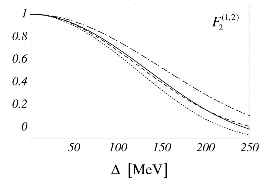
Figure 9:

References

- [1]
- [2] E. Hayward, Radiat. Phys. Chem. 41 (1993) 739
- [3] M. Schumacher, A.I. Milstein, H. Falkenberg, K. Fuhrberg, T. Glebe, D. Häger and M. Hütt, Nucl. Phys. A576 (1994) 603
- [4] D. Häger, K. Fuhrberg, T. Glebe, M. Hütt, M. Ludwig, M. Schumacher, B.-E. Andersson, K. Hansen, B. Nilsson, B. Schröder, L. Nilsson, E. Kuhlmann and H. Freiesleben, Nucl. Phys. A595 (1995) 287
- [5] D.H. Wright, P.T. Debevec, L.J. Morford, A.M. Nathan, Phys. Rev. C32 (1985) 1174
- [6] M. Rosa-Clot and M. Ericson, Z. Phys. A320 (1985) 675
- [7] M. Ericson, Z. Phys. A324 (1986) 373
- [8] M. Schumacher, P. Rullhusen and A. Bauman, Il Nuovo Cim. 100A (1988) 339
- [9] M.-Th. Hütt and A.I. Milstein, Nucl. Phys. A609 (1996) 391
- [10] G. Feldman, K. E. Mellendorf, R. A. Eisenstein, F. J. Federspiel, G. Garino, R. Igarashi, N. R. Kolb, M. A. Lucas, B. E. MacGibbon, W. K. Mize, A. M. Nathan, R. E. Pywell, and D. P. Wells,, Phys. Rev. C54 (1996) 2124 R
- [11] H. Falkenberg, K. Fuhrberg, T. Glebe, D. Häger, A. Hünger, M. Hütt, A. Kraus, M. Schumacher and O. Selke, in: “Mesons and Nuclei at Intermediate Energies”, Dubna, Russia,1994, Mikhail Kh. Khankhasayev and Zh.B. Kurmanov Eds., World Scientific 1995
- [12] A. Molinari, Phys. Rep. 64 (1980) 283
- [13] B. Ziegler, in: NATO ASI Series B 142 (1985) 293
- [14] J.S. Levinger and H.A. Bethe, Phys. Rev. 78 (1950) 115
- [15] J.L. Friar, Phys. Rev. Lett. 36 (1976) 510
- [16] H. Arenhövel, in: NATO ASI Series B 142 (1985) 251
- [17] S.-O. Bäckman, G.E. Brown, J.A. Niskanen, Phys. Rep. 124 (1985) 1
- [18] T. Ericson, W. Weise, “Pions and Nuclei”, Oxford Univ. Press 1988
- [19] D.O. Riska, Phys. Rep. 181 (1989) 207
- [20] A.Arima, G.E.Brown, H.Hyuga and M.Ichimura, Nucl. Phys. A205 (1973) 27
- [21] W.T. Weng, T.T.S. Kuo and G.E. Brown, Phys. Lett. 46B (1973) 329
- [22] G.E. Brown and M. Rho, Nucl. Phys. A338 (1980) 269
- [23] G.E. Brown, in: “Symmetries and fundamental interactions in nuclei”, E. Henley and W. Haxton Eds., World Scientific 1995
- [24] M. Ericson and M. Rosa-Clot, Phys. Lett. B188 (1987) 11
- [25] K.P. Schelhaas, J.M. Henneberg, M. Sanzone-Arenhövel, N. Wieloch-Laufenberg, U. Zurmühl, B. Ziegler, M. Schumacher and F. Wolf, Nucl. Phys. A489 (1988)189
- [26] K. Fuhrberg, G. Martin, D. Häger, M. Ludwig, M. Schumacher, B.-E. Andersson, K.I. Blomqvist, H. Ruijter, B. Sondell, E. Hayward, L. Nilsson, B. Schröder and R. Zorro, Nucl. Phys. A548 (1992) 579
- [27] P. Christillin and M. Rosa-Clot, Nuov. Cim. 43A (1978) 172
- [28] P. Christillin and M. Rosa-Clot, Nuov. Cim. 28A (1975) 29
- [29] W.A. Alberico and A. Molinari, Z. Phys. A309 (1982) 143
- [30] K. Fuhrberg, D. Häger, T. Glebe, B.-E. Andersson, K. Hansen, M. Hütt, B. Nilsson, L. Nilsson, D. Ryckbosch, B. Schröder, M. Schumacher and R. Van de Vyver, Nucl. Phys. A591 (1995) 1
- [31] T. deForest and J.D. Walecka, Adv. Phys. 15 (1966) 1
- [32] S.B. Gerasimov, Phys. Lett. 13 (1964) 240
- [33] H. Arenhövel, Z. Phys. A297 (1980) 129
- [34] M.R. Anastasio and G.E. Brown, Nucl. Phys. A285 (1977) 516
- [35] C.W. deJager, H. deVries and C. deVries, Nucl. Data Tables 14 (1979) 479