The importance of initial-final state correlations for the formation of fragments in heavy ion collisions
P.-B. Gossiaux^1,2 and J. Aichelin¹

¹ SUBATECH
Université de Nantes, EMN, IN2P3/CNRS F-44072 Nantes, France
² National Superconducting Cyclotron Laboratory, MSU, USA

Using quantum molecular dynamics simulations, we investigate the formation of fragments in symmetric reactions between beam energies of E = 30A MeV and 600A MeV. After a comparison with existing data we investigate some observables relevant to tackle equilibration: $\mbox{d}\sigma/\mbox{d}E_{rat}$, the double differential cross section $\mbox{d}^{2}\sigma/p_{t}\mbox{d}p_{z}\mbox{d}p_{t}$,… Apart maybe from very energetic ($\mbox{E}\geq\mbox{400A~{}MeV}$) and very central reactions, none of our simulations gives evidence that the system passes through a state of equilibrium. Later, we address the production mechanisms and find that, whatever the energy, nucleons finally entrained in a fragment exhibit strong initial-final state correlations, in coordinate as well as in momentum space. At high energy those correlations resemble the ones obtained in the participant-spectator model. At low energy the correlations are equally strong, but more complicated; they are a consequence of the Pauli blocking of the nucleon-nucleon collisions, the geometry, and the excitation energy. Studying a second set of time-dependent variables (radii, densities,…), we investigate in details how those correlations survive the reaction especially in central reactions where the nucleons have to pass through the whole system. It appears that some fragments are made of nucleons which were initially correlated, whereas others are formed by nucleons scattered during the reaction into the vicinity of a group of previously correlated nucleons.

PACS numbers: 25.75.+r, 25.70.Pq.

1 Introduction

The multifragmentation of nuclei excited in collisions with protons or heavy ions is one of the most interesting and challenging topics in present-day heavy-ion physics. The production of intermediate mass fragments (IMF), which we define as objects with $3\leq Z\leq 25$, in collisions of a proton with heavy targets was first observed about 40 years ago [1]. Using radiochemical methods, however, a total cross section for fragmentation could not be determined and this process had been considered as quite rare and exotic.

A decade ago two findings, one experimental and one theoretical, have placed multifragmentation into the spotlight. Bombarding large target nuclei with heavy ions Warwick et al. [2] found that many IMFs are produced simultaneously and that multifragmentation is the dominant reaction channel at beam energies larger than 35A MeV. Observing that the mass yield curve approximately obeys a power law $\sigma(A)\propto A^{-\tau}$, the Purdue group [3] conjectured that multifragmentation is a clear signature [4] for the phase transition between a gaseous and a liquid phase of nuclear matter. This transition is predicted to occur around a density of $0.4\rho_{0}$, $\rho_{0}$ being the normal nuclear-matter density.

Since then, the study of multifragmentation has been considered of such interest that special ($4\pi$) detectors have been designed to inspect this process in detail. Today it is a major research project at all heavy ion accelerators. However, despite these extensive experimental efforts, the underlying physical mechanism remains unclear and the debate is still quite controversial. This is due to the fact that the experiments have revealed many puzzling aspects. Some results are in perfect agreement with the conjecture that the fragments are emitted from a globally thermalized system. Others, however, can hardly be reconciled with this conjecture. We will summarize these results shortly.

It has been observed that independently of the mass of the projectile-target combination, the form of the mass yield curve [5] is almost identical from 30A MeV up to the highest energies. The form observed is that expected for formation of fragments in a liquid-gas phase transition. Other observables show, however, that the underlying process changes. At low beam energies the slopes of the energy spectra of protons and IMFs agree, whereas, starting from about 100A MeV, an increasing difference of the slopes is observed [6]. This has been interpreted as an evidence that, at low energy, the whole nucleus takes part in the multifragmentation to the limit that the process can be described as a compound nucleus decay, whereas, at high energies, only the spectators’ part contributes significantly [5].

The backward energy spectra of fragments are found to be rather independent of the beam energy [2, 7] and of the projectile mass [2] (for $A_{\rm P}\leq 20$). At each angle the spectra have the form expected for a thermal emission from a moving source. Thus single arm experiments seem to indicate an emission from a thermal source. If one compares the spectra observed under different angles [2, 6] one finds, however, that the source velocity, the Coulomb barrier and the temperature depend on the observation angle [8]. This contradicts the thermal source assumption.

Recent experiments performed with a $4\pi$ detector have revealed that the energy balance in central collisions is dominated by a large undirected flow component ($\beta\approx 0.1c$) and that the Coulomb repulsion and the possible thermal energy represent only a minor part [9]. Hence the nucleus seems to explode.

The models advanced to describe multifragmentation invoke practically all imaginable physical processes. For a recent review we refer to [5]. Most of the phenomenological models only aim to explain/reproduce a few observables. In the last years, they have been superseded by numerically involved models which predict results for a multitude of observables simultaneously. Presently, these models can be classified into two main categories.

First, statistical models [10, 11, 12] which neglect the dynamics of the reaction by supposing that the system or a subsystem reaches equilibrium in the course of the reaction and maintains this equilibrium until its density has decayed to approximately 0.4 $\rho_{0}$. According to this assumption, all possible exit channels (consisting of nucleons and—possibly excited—fragments) are populated with equal probabilities. These models have revealed themselves to reproduce mass yields, fragment multiplicities and fragment-mass correlations very accurately for 800 A MeV reactions [13] but fail to reproduce dynamical variables [9, 14], a fact not yet understood.

A second type of approach is the quantum molecular dynamics (QMD) [15] model which follows the time-evolution of the full multi-nucleon phase space distribution from the initial collision of projectile and target up to the final formation of fragments. This model is more ambitious than the statistical approach. First, the QMD model permits to check whether complete equilibrium is reached for a given reaction. When thermal equilibrium is established, it has been shown that the QMD model predicts the same fragment multiplicities as the statistical models [23]. However, it also predicts the density and the temperature which are just input parameters in thermal models. When complete equilibrium is not reached, it allows to investigate the reaction as well. For this reason, we claim that the QMD model goes beyond the thermal ones. On the other hand, there are some drawbacks attached to the QMD approach. For instance, it usually requires more approximations than the statistical models, as discussed in section 2.1… Nevertheless, let us mention from the beginning that QMD results reproduce the experimental data fairly well, as it will be detailed in section 2.4.

Even though this agreement is primordial, the numerous physical processes included in the QMD code and the abundance of degrees of freedom very often prevent us to get a clear view of the relevant underlying physics and of the causal links. But the physics of heavy ion collisions should not reduce to a black box with tuning parameters: At some point, one has to understand the reaction mechanisms in a coherent, comprehensive and preferably conceptual manner.

It is precisely the goal of this paper to make some steps towards a more global understanding of nucleus-nucleus collisions and their energy dependence (from basically 50A MeV to 600A MeV), by analyzing the reaction as a function of time and by probing some specific time-correlations (that we shall sometimes simply denote “correlations” when no ambiguity exists). Quite generally, we shall speak of time-correlation if nucleons belonging to a specific class of emitted fragments have a different mean history than all nucleons considered indiscriminatingly. A very good (but trivial) example of such a time-correlation can be found in the participant spectator (PS) model: At high energy and finite impact parameter, experimental and theoretical results suggest that the system can be divided into two subsystems, the spectators and the participants. According to this model, the nucleons which compose the heavy fragments would mainly emerge from the spectator zones, so avoiding the fireball.

One easily realizes that the analysis of time-correlations is particularly useful to clarify whether the system has passed through a state of global equilibrium before (multi)fragmenting. If it were the case, all the memory would be completely lost and time-correlations would disappear. However, we will find many of them, strong and not only of geometrical nature. This indicates that inside the QMD approach, the system does not pass through a state of global equilibrium.

Not only time-correlations act as a touchstone of the system’s equilibration but they also play a first role in understanding (a)the mechanisms of fragment formation as well as (b)the way the memory of the entrance channel partly survives the high density/temperature phase of the heavy ion reaction. We will illustrate this assertion by analyzing the time-evolution of some well-chosen quantities, like the radius of prefragments, their internal kinetic energy,…

The paper is organized as follows: In section 2, we briefly introduce the QMD model (2.1), discuss more extensively some of its aspects relevant in the context of fragmentation (2.2) and state our conventions 2.3. Next (2.4), we validate the model by comparing it to recent experimental results obtained at MSU, GANIL and GSI. In section 3, we present a survey of some typical reactions, what will help the reader to get a general idea of the propagation of prefragments at intermediate times. In Section 4, we investigate to what degree the system achieves global equilibration. We present results for the stopping, the double differential cross section ${\mbox{d}^{2}\sigma/p_{t}\mbox{d}p_{t}\mbox{d}p_{z}}$ and the mixing of projectile and target nucleons, which suggest a small degree of equilibration. In Section 5, we detail the initial-final state correlations for symmetric systems between 50A MeV and 400A MeV. After outlining the method employed to construct these correlations (5.1), we address both cases of coordinate and momentum spaces. We find strong correlations between the final fate of the nucleons and their initial position in phase space. Moreover, we have distinguished two classes of fragments (those finally located (a) around mid-rapidity and (b) around target or beam rapidity)… and discovered additional correlations. In section 6, we inspect how these correlations can be preserved during the time-evolution of the system, especially for the nucleons which traverse the whole reaction partner. We conclude our work in section 7.

2 The QMD model

2.1 Description of the approach

In the QMD model, the time evolution of the system is calculated by means of a generalized variational principle: After having chosen a test wave function $\phi$ (which contains time-dependent parameters), one evaluates the action

$$S=\int\limits^{t_{2}}_{t_{1}}{\cal L}[\phi,\phi^{\ast}]dt$$ (1)

with the Lagrange functional ${\cal L}$

$${\cal L}=\left\langle\phi\left|i\hbar{\frac{d}{dt}}-H\right|\phi\right\rangle\;,$$ (2)

where the total time derivative includes the derivation with respect to the parameters. The time evolution of the parameters is then obtained by requiring the action to be stationary under the allowed variation of the wave function. This requirement leads to an Euler-Lagrange equation for each time-dependent parameter.

If the true solution of the Schrödinger equation is contained in the set of wave functions $\phi$, this variational method of the action provides the exact solution of the Schrödinger equation. If the parameter space is too restricted, one obtains the closest wave function to the exact solution (in that restricted parameter space).

The basic assumption of the QMD model is that a test wave function of the form

$$\phi=\prod_{\alpha=1}^{A_{P}+A_{T}}\phi_{\alpha}$$ (3)

with

$$\phi_{\alpha}(x_{1},t)=\left({\frac{2}{L\pi}}\right)^{3/4}\,e^{-(x_{1}-x_{\alpha}(t)-p_{\alpha}(t)t/m)^{2}/L}\,e^{i(x_{1}-x_{\alpha}(t))p_{\alpha}(t)}\,e^{-ip_{\alpha}^{2}(t)t/2m}$$ (4)

and

$$\hbar,c=1$$ (5)

is a good approximation to the nuclear wave function. Neglecting antisymmetrization is the most drastic approximation of the model , as, for instance, all properties related to shell structures cannot be accounted for.

The wave function $\phi_{\alpha}$ has two time-dependent parameters: $x_{\alpha}(t),p_{\alpha}(t)$, while L is fixed. The initial values of these parameters are chosen in such a way that the ensemble of $A_{T}$ + $A_{P}$ nucleons gives proper densities and momentum distributions of the projectile and target nuclei.

For the coherent states $\phi_{\alpha}$ and the Hamiltonian

$$H=\sum_{i}T_{i}+{\frac{1}{2}}\sum_{ij}V_{ij}\;,$$ (6)

where $T_{i}$ is the kinetic energy and $V_{ij}$ the potential energy between two nucleons, the Lagrangian and the variation can be easily evaluated:

$${\cal L}=\sum_{\alpha}\biggl{[}\dot{x_{\alpha}}p_{\alpha}-{1\over 2}\sum_{\beta}\langle V_{\alpha\beta}\rangle-{\frac{3}{2Lm}}\biggr{]}$$ (7)

$$\dot{\bar{x}}_{\alpha}={\frac{p_{\alpha}}{m}}+\nabla_{p_{\alpha}}\sum_{\beta}\langle V_{\alpha\beta}\rangle$$ (8)

$$\dot{p}_{\alpha}=-\nabla_{\bar{x}_{\alpha}}\sum_{\beta}\langle V_{\alpha\beta}\rangle$$ (9)

with

$${\bar{x}_{\alpha}}=x_{\alpha}+{\frac{p_{\alpha}}{m}}t$$ (10)

and

$$<V_{\alpha\beta}>=\int d^{3}x_{1}d^{3}x_{2}<\phi_{\alpha}\phi_{\beta}|V(x_{1},x_{2})|\phi_{\alpha}\phi_{\beta}>.$$ (11)

These are the time evolution equations to be solved numerically. The interaction $V_{ij}$ is taken as the real part of the Brückner g-matrix supplemented by the Coulomb interaction. If the energy is sufficiently high, the g-matrix becomes complex and the imaginary part acts like a cross section. Details may be found in [15].

The variational approach reduces the complicated task to follow the time evolution of a n-body wave function to the resolution of $6\,n$ coupled differential equations for the centroids of the coherent state wave functions in coordinate and momentum space. In the following, we shall sloppily call these centroids position and momentum of the nucleons. However, for any rigorous interpretation, one has to keep in mind that these are just parameters of a wave function which indeed obeys the uncertainty principle.

This approach also allows a very convenient definition of clusters: At the end of the simulation the average phase space occupation is quite low. Hence only nucleons with mutual interactions, i.e. the ones forming a fragment are close together in coordinate space. A simple minimum-spanning-tree algorithm, applied to the centroids of the coherent states, permits to define the clusters. If the average phase-space occupation is sufficiently low the result is quite independent of the minimum-spanning-tree radius.

The QMD model has been extensively discussed in a recent Physics Reports [15]. Later the results have been updated in other reviews [16, 17]; therefore we do not repeat further details here. Let us just discuss a few important points concerning fragmentation and time-correlations.

2.2 Aspects of the QMD model specific to fragmentation and time-correlations

1. We employ a direct product of coherent states. Hence, one may in principle find more than one particle in a unit cell $h^{3}$ of the phase space although this is forbidden for the one-body phase space density by the Liouville theorem. To avoid a possible overoccupation one has sometimes introduced a potential depending on the relative momenta and the relative positions of the particles. This so called Pauli potential provides a well defined nuclear ground state which corresponds to the minimum of the Hamiltonian used in the calculation. For an isolated nucleus, the nucleons carry their proper Fermi momentum but they do not move relatively to the center of mass (${dx_{i}/dt}=0$). Hence the price one has to pay is the crystallization of the cold nucleus: Nothing else but a collective motion is possible. Indeed, if just one nucleon is moved, it enters an already occupied cell. Due to this crystallization the fragments are excited for a much longer time than in the standard QMD (the one we use in this paper), where the fragments are practically cold after 180 fm/c. Therefore, a so called afterburner, i.e. a statistical evaporation program, has to be used at the end of the reaction to deexcite the hot fragments into their ground state. These two approaches (QMD with Pauli potential + afterburner and standard QMD) are conceptually different and naturally lead to fragmentation patterns that also differ quite substantially [18].

2. The QMD parameterization turns out to be very useful if one is interested in following the flow of matter. Indeed, inside the model, the one-body density is

$$\rho\left(x,t\right)=\sum_{\alpha=1}^{A_{P}+A_{T}}\left|\phi_{\alpha}\left(x,t\right)\right|^{2}\;.$$ (12)

As all the $\phi_{\alpha}$ are peaked around their centroids, one easily figures out how nuclear matter evolves from one point to another by just following the centroid distribution. For instance, tagging nucleons as projectile or target-like, one can study how efficiently they mix in the course of the reaction. Of course, in nature, particles are indistinguishable and attaching such a flag of origin to each particle seems a bit unrealistic. However, by going to the Wigner density formalism, we can interpret the time evolution of the Schrödinger equation as the flow of the phase space density. This allows us to investigate the (mean) origin of the matter contained in the final fragments. In this context, particles merely serve as an expedient to calculate that flow of matter .

3. Another delicate point where the unsatisfactory treatment of that indistinguishable character may cause some trouble are the nucleon-nucleon collisions. In standard QMD, the scattering angle in the nucleon-nucleon center of mass system ($\theta_{cm}$) is always taken lower than $\pi/2$. At the large energy limit, this is justified, as we know that a transfer of large longitudinal momentum is improbable: In proton-neutron collisions, $\theta_{cm}$ almost never exceeds $\pi/2$. To assume a similar constrain in proton-proton and neutron-neutron collisions is therefore acceptable. In more technical terms, the nucleon-nucleon scattering amplitude basically contains 2 contributions: the t and the u channels. At high energy, the t channel dominates by far: the outgoing forward nucleon has a high probability to be the same particle as the ingoing forward nucleon.

On the contrary, at lower energy, both scattering amplitudes associated with the t and u channels become independent of $\theta_{cm}$, and the differential cross section is almost isotropic. Accordingly, one should in principle remove that $\theta_{cm}\leq\pi/2$ constrain from the model and let $\theta_{cm}$ range from $0$ to $\pi$. This modification has no consequence on the final state of the reaction (number, masses and momenta of the fragments) but may change dramatically the time-correlations and our mental representation of the reaction evolution.

Of course, one can also take the “information” point of view: a nucleon-nucleon collision happening exactly at $\theta_{cm}=\pi$ leaves the physical state unchanged. The forward (respectively backward) outgoing nucleon transmits the memory of the forward (respectively backward) ingoing nucleon. Only a collision with a finite $\sin\left(\theta_{cm}\right)$ is able to change the physical state. Hence, to study how efficiently the collisions destroy the memory of the system, maintaining $\theta_{cm}\leq\pi/2$ is not so unrealistic as it may appear at first sight.

Which one of these two conventions should we adopt? At very high energy ($E\geq\mbox{1 GeV}$), this question is irrelevant. On the other hand, at very low energy ($E\leq\mbox{100 MeV}$) one can invoke the Pauli-blocking of the collisions which should be strong enough to reduce the number of collisions significantly and solve the dilemma. Unfortunately, for energies ranging between those two values, the problem shows up. We have chosen the following approach: for the main discussion, we shall stick to the standard QMD and $\theta_{cm}\in[0,\pi/2]$ (called hereafter “model (A)”). Occasionally, some crucial quantities will be reevaluated in the “$\theta_{cm}\in[0,\pi]$” version of QMD (called hereafter “model (B)”) and compared to the results obtained in model (A).

Hereafter, we state the other underlying conventions and clarify the few non-standard terms used in this paper:

2.3 Conventions

• the results are displayed in the nucleus nucleus center of mass system

• the beam axis is in z direction, the impact parameter points into the x direction

• the projectile has initially a positive z momentum and is displaced (for non zero impact parameters) in the positive x direction

• A soft equation of state [15] has been used. Consequently, for some observables (i.e. flow), one does not expect to have quantitative agreement with experiment.

• Whenever they appear, the following symbols are to be understood as defined hereafter:

  $$b_{<} \equiv$$ 3 fm for all systems

  $$b_{>} \equiv \left\{\begin{array}[]{l}\mbox{6~{}fm for Xe~{}+~{}Sn}\\ \mbox{8~{}fm for Au~{}+~{}Au}\end{array}\right.$$

  LF $$\equiv 2\leq A\leq 4$$ light fragment: any single or fragment of mass

  HF $$\equiv A\geq 5$$ heavy fragment: any fragment of mass

2.4 The QMD model compared to experiment

As we have explained, the quest for correlations between the initial and the final state of a heavy ion reaction is meaningful only if the model employed contains the essential physics. To check that QMD basically satisfies this requirement, extensive calculations have been performed and compared to the most demanding data recently measured with 4 $\pi$ detectors at GSI, MSU and GANIL. The data obtained at these facilities are to a large extend still preliminary, so that the conclusions we draw should not be considered as definitive.

In figure 1, we present two quantities fundamental for the multifragmentation: the intermediate mass fragment (IMF) multiplicity and the number of charged particles ($\mbox{N}_{C}$) as a function of the beam energy (E) for the Kr + Au system at 3 different energies (from 55A MeV up to 200A MeV). In this figure, the experimental data obtained by the MSU collaboration [20] and the filtered QMD-calculations are confronted, with good overall agreement.

In figure 2, we present another important quantity: the percentage of nucleons bound in fragments $Z\geq 3$. It has been measured experimentally for the Au + Au system by the FOPI collaboration. Although not displayed, the maximum percentage is obtained for beam energies around 50A MeV. Also, one notices a rapid decrease at high energy. QMD reproduces the low-energy value, but for E = 400A MeV, this is no longer the case… In fact, it is well-known that for energies larger than 400A MeV, the present version of the QMD model fails to describe the IMF multiplicity [22] (although the dependence of the number of nucleons bound in clusters as a function of the $\mbox{N}_{C}$ is correctly reproduced). The reason is not yet understood… However, one could demonstrate that this failure is not due to the thermal properties of the QMD nuclei but more likely related to the low momentum transfer to the spectators [23]. It is also true that statistical models succeed in describing these mass yields [13]. Nevertheless, they take the freedom to adjust the excitation energy of the system by hand, while in the QMD approach, it is completely determined by the solution of the time-evolution equations.

In figure 3, we present a more refined signature of the multifragmentation: the IMF multiplicity as a function of $\mbox{N}_{C}$, for some of the reactions studied in figure 1. At all energies (from 55A MeV up to 200A MeV), a good agreement between theory and experiment is achieved. A fair agreement has also been obtained for the recent measurements performed with the INDRA detector at GANIL (figure 4). The deviations observed at small $\mbox{N}_{C}$ may have two origins: (1) the filter routines are still preliminary and/or (2) collisions at large impact parameter are more difficult to describe theoretically.

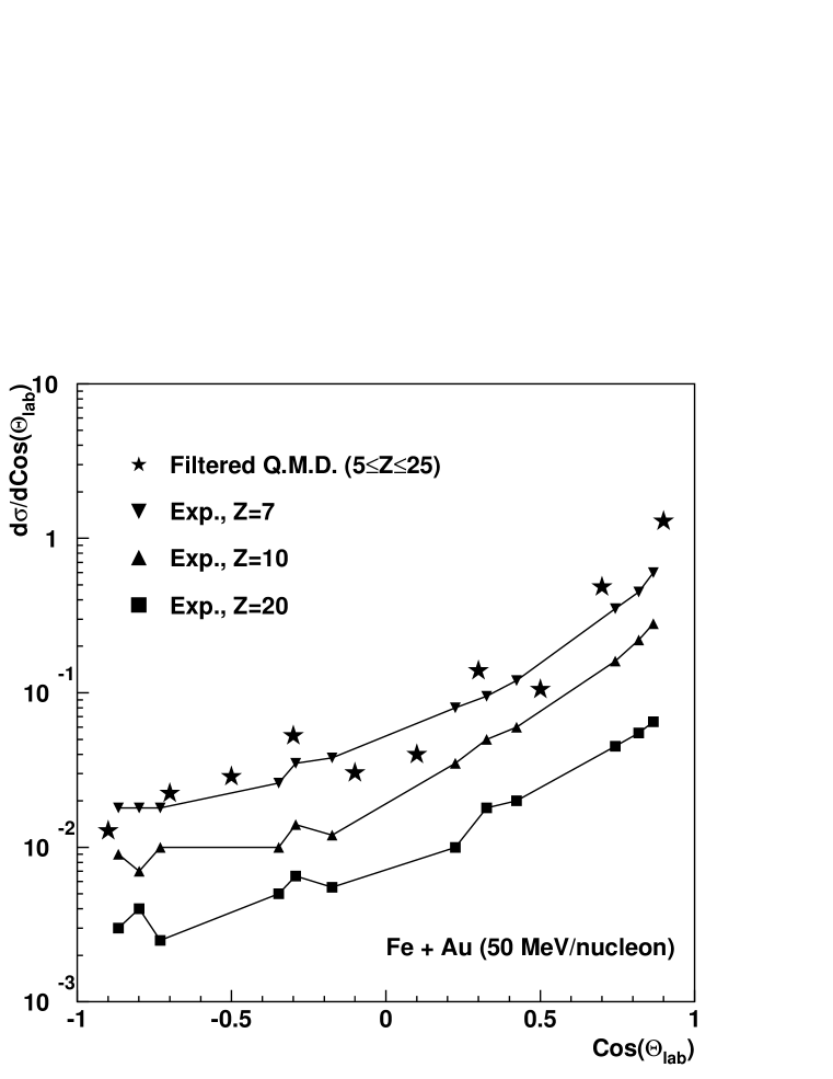
Figure 5: Angular distribution of fragments in the Fe + Au reactions at 50A MeV. The experimental angular distribution for Z = 7, 10 and 20 are compared with filtered QMD results for the angular distribution of all fragments $5\leq\mbox{Z}\leq 25$.

An even more detailed investigation of a 50A MeV reaction is available for the asymmetric system Fe + Au, where the angular distribution of the fragments has been measured [21]. The comparison with the QMD calculation is displayed in figure 5 (in the case of QMD, we have summed over all fragments with $Z\in[5,20]$, in order to obtain sufficient statistics). The angular distribution of the fragment yield turns out to be nicely reproduced. The absolute value is also in reasonable agreement.

Somehow, this overall agreement obtained at the lowest beam energy is surprising: In this regime, at least some of the approximations made to derive the QMD equations are not valid anymore. These approximations include the quasi particle approximation, the neglect of interference effects between subsequent collisions (the particles behave like classical billiard balls) and the assumption that the Pauli blocking of nucleon scattering can be properly modeled,… Nevertheless, what we will retain from these comparisons is the increasing evidence that for non-peripheral reactions ranging from 30A MeV to 400A MeV, the QMD model describes the measured data satisfactorily.

3 Survey of the reaction

We start our theoretical investigations with a survey of some reactions we will encounter later on. We illustrate three cases where typical reaction scenarios are expected: the participant spectator (PS) scenario (Au + Au, 600A MeV, 8 fm), the multifragmentation (MF) scenario (Au + Au, 150A MeV, 3 fm) and the incomplete fusion (IF) scenario (Xe + Sn, 50A MeV, 3 fm). Later, we will discuss in more details to which extent those scenario indeed match our numerical simulations.

For those three reactions, we select one single event and plot, in figure 6, the time sequence of the density profiles projected onto the $xz$ plane. Each nucleon is marked by a circle of 1.5 fm radius. Hence circles which are overlapping belong to the same cluster (although the projection may fool a little bit). We see three quite different exit channels. The 600A MeV collision shows fragments only around the projectile and target rapidities, as if those fragments emerge from the spectator matter. At 150A MeV, we already find fragments at mid-rapidity. The pattern of particle emission seems isotropic (but future analysis will reveal it is not quite so). At 50A MeV, we observe distinct projectile and target-like-fragments as well as mid-rapidity fragments which are clearly separated in momentum and coordinate space.

To conceive plausible scenarios of the reactions, one has to understand more precisely how the fragments emerge. In fact, one can already get valuable information by studying the evolution of the mean center of mass of all the nucleons emerging asymptotically in a given fragment. Let us stress that at intermediate times, these nucleons can be very dispersed in phase-space. To avoid confusing the reader, we will use the word “prefragment” to denote this ensemble. For each prefragment, let us label $A_{p}$ (resp. $A_{t}$) the number of nucleons initially contained in the projectile (resp. target) and emitted in the asymptotic fragment . One has of course $A_{p}+A_{t}=A$, the mass of the fragment. Next, we define

• The center of mass and mean momentum per nucleon of the prefragment as

  $$\vec{R}(t)=\frac{\sum_{i=1}^{A}\vec{r_{i}}(t)}{A}\mbox{ and }\vec{P}(t)=\frac{\sum_{i=1}^{A}\vec{p_{i}}(t)}{A}\;,$$ (14)

  respectively. In definition 14, $\vec{r}_{i}(t)$ is the position of the $i^{th}$ prefragment’s nucleon at time t and $\vec{p}_{i}(t)$ its momentum.

• The center of mass of projectile/target nucleons and their mean momentum per nucleon:

  $$\vec{R}_{p/t}(t)=\frac{\sum_{i_{p/t}=1}^{A_{p/t}}\vec{r}_{i_{p/t}}(t)}{A_{p/t}}\mbox{ and }\vec{P}_{p/t}(t)=\frac{\sum_{i_{p/t}=1}^{A_{p/t}}\vec{p}_{i_{p/t}}(t)}{A_{p/t}}\;,$$ (15)

  where $\vec{r}_{i_{p/t}}(t)$/$\vec{p}_{i_{p/t}}(t)$ is the position/momentum of the $i_{p/t}^{th}$ projectile/target nucleon at time t.

Then, we perform the average (denoted by $\overline{\vphantom{X}...}$) over all fragments, possibly selecting a given class, and over a large ensemble of QMD events. From figure 6, it is obvious that 3 subclasses of heavy fragments have to be privileged:

• The heavy fragments emerging around the projectile rapidity, referred hereafter as projectile-like-fragments (PLF).

• The heavy fragments emerging around the target rapidity, referred hereafter as target-like-fragments (TLF).

• The heavy fragments emerging at mid-rapidity, referred hereafter as mid-rapidity fragments (MRF).

In figure 7, we present $\overline{X}_{p}(t)$ as a function of $\overline{Z}_{p}(t)$ in Au + Au (400A MeV, 3 fm) and Xe + Sn (50A MeV, 3 fm) reactions, for those three subclasses. In the case of MRFs, we have limited ourselves to those fragments emerging with $P_{z}\left(t_{fin}\right)>0$, to avoid trivial cancellations.

At 400A MeV, we observe strong transverse correlations, in agreement with a (refined) PS model: basically, the projectile nucleons which emerge in PLFs are initially lying in the projectile spectator-zone, so avoiding the target. Looking more carefully at the data, one notices that these nucleons have, at initial time, a finite mean momentum in $x$ direction. We have evaluated $\overline{P_{x}}^{PLF}(t=0)\approx\mbox{20 MeV/c}$, which is already an appreciable fraction of the directed flow observed experimentally.

The projectile nucleons emerging in TLFs are located on the other face of the projectile nucleus, where they will be ripped off more easily by the target spectators. They also possess a finite transverse momentum, in the $-x$ direction, which helps them in that respect.

As expected, MRFs’ nucleons are lying in the participant region. In the course of the reaction, they are stopped and gain transverse momentum by interacting with surrounding nucleons; one may conjecture that this is the onset of the blast wave observed recently in very central collisions [9].

At 50A MeV, the situation is quite different. Firstly, no more spatial transverse correlation is observed. As a matter of fact, the clear-cut PS model supporting them naturally looses its validity at low energy.

Secondly, the blast has completely disappeared because the dynamics is now dominated by the attractive part of the mean-field potential. Even if nucleons emerging in PLFs and MRFs are still momentum-preselected and tend to point out of the overlapping region, they are bent in the course of the reaction by their strong attractive interaction with the nucleons of the other classes; therefore, we observe ultimately an even larger flow in the $-x$ direction . Hence, the projectile and target have a tendency to rotate around a common axis; this seems to be the onset of the deep inelastic collision (DIC) regime, encountered at higher impact parameters. Let us remind that, according to the DIC scenario, MRFs’ nucleons equilibrate and reside almost exactly at the center of mass, while PLFs’ nucleons rotate at the periphery and are only emitted once this rotation has taken place.

Nevertheless, figure 7 clearly proves that for a beam energy of 50A MeV and an impact parameter of 3 fm, PLFs’ projectile nucleons traversed the whole target nucleus more than rotated around it (and vice versa). In fact, they followed the same trajectory as MRFs’ nucleons but went on farther for a reason still unclear at this stage—if any reason at all—other than a statistical fluctuation. This “transparency” must be strongly contrasted with the high energy case, where PLFs’ nucleons come (almost) exclusively from the spectator parts. We will discuss this phenomenon in more details later.

4 Does the whole system equilibrate?

Ideally, one should test the phase space occupation in the exit channels to answer this question. However, their number makes this ideal test impossible in practice. Therefore, we limit ourselves to check whether some necessary criteria are satisfied:

4.1 Equilibration according to $E_{rat}$

In a thermalized system, the momenta distribution must be isotropic. For a nucleus-nucleus collision, the original longitudinal anisotropy has first to be destroyed by nucleon-nucleon interactions. Hence, an isotropic distribution of emitted matter is not trivially achieved. For instance, figure 6 already shows qualitatively that the stopping may be only partial.

Possible anisotropy can be quantified by the differential cross section $d\sigma/dE_{rat}$, where Erat is defined as

$$E_{rat}={\sum p_{\perp}^{2}/2m_{N}\over\sum p_{z}^{2}/2m_{N}}.$$ (16)

Equilibration corresponds to $E_{rat}=2$. This quantity has been measured at 150A MeV by the FOPI collaboration and compared with QMD (cf. figure 8). The agreement demonstrates that for central collisions (the calculation was stopped at b = 7 fm) the excitation energy of the system is properly described in the QMD model. The acceptance cuts of the detector lower the $E_{rat}$ values as compared to the QMD events in which all particles are counted. However, independently of the acceptance, one can formulate the general statement that $E_{rat}=2$ and global equilibration are achieved only in rare events at that energy We have evaluated $d\sigma/dE_{rat}$ at lower energies (Xe + Sn at 32 and 50A MeV), where data have been taken but not analyzed yet. At large values of $E_{rat}$, we observe about the same slope as for the 150A MeV reaction. Consequently, $E_{rat}$ values larger than 1.5 are almost never obtained.

Of course, one can argue that experimentally, all impact parameters are mixed, whereas the physics can differ sensibly from small to large impact parameter. For instance, in the PS model taken at finite impact parameter, one may conjecture that the participants equilibrate, but the spectators certainly do not. A global thermalization is therefore unrealistic. On the other hand, for very small $b$, no more nucleon can be considered as a spectator and global equilibrium might be achieved. This motivates us to investigate the dependence of $d\sigma/dE_{rat}$ on $E$ and $b$. For each fixed value of $b$, $d\sigma/dE_{rat}$ turns out to be relatively peaked around its mean value ($\overline{E}_{rat}$), displayed in table 1, for Au + Au and Xe + Sn reactions at 50, 150, 400A MeV and 50A MeV respectively.

For nearly all energies and impact parameters, $\overline{E}_{rat}\ll 2$. This discards the global equilibrium hypothesis. Only for E larger than $\approx 400$ A MeV, one might come close to global equilibration in very central collisions (which however do not contribute significantly to the total cross section). Moreover, if one remembers the dependence of the IMF multiplicity on the beam energy (in figure 1), one can infer that global equilibrium is seldom found simultaneously with multifragmentation.

For all energies, a higher impact parameter results in a higher anisotropy of the momentum distribution. But this is particularly true at high energies, where the initial transverse position of a nucleon is a strong prerequisite to its destiny. At lower energies, such a geometrical criteria is not expected, and the dependence of $\overline{E}_{rat}$ on $b$ is indeed weaker.

We have just observed and understood that a global equilibrium cannot be achieved at large E and large b. One can wonder why such a conclusion holds at small E ($\approx 50$ A MeV) at all. This is precisely one of the concerns of this paper. However, without going much further, one realizes that at the same energy and same $\hat{b}=b/R$, $\overline{E}_{rat}$ is smaller for the Xe + Sn system than for the Au + Au one,… a natural feature in the interaction of non-opaque objects.

4.2 Equilibration according to the momentum distribution of specific fragments

In the previous section, it was shown that the momentum distribution of emitted particles was globally anisotropic. But is it true for each particle species? For instance, the thermal form of the single particle spectra gave rise to speculations that the system may have thermalized, in apparent contradiction with what we have just deduced.

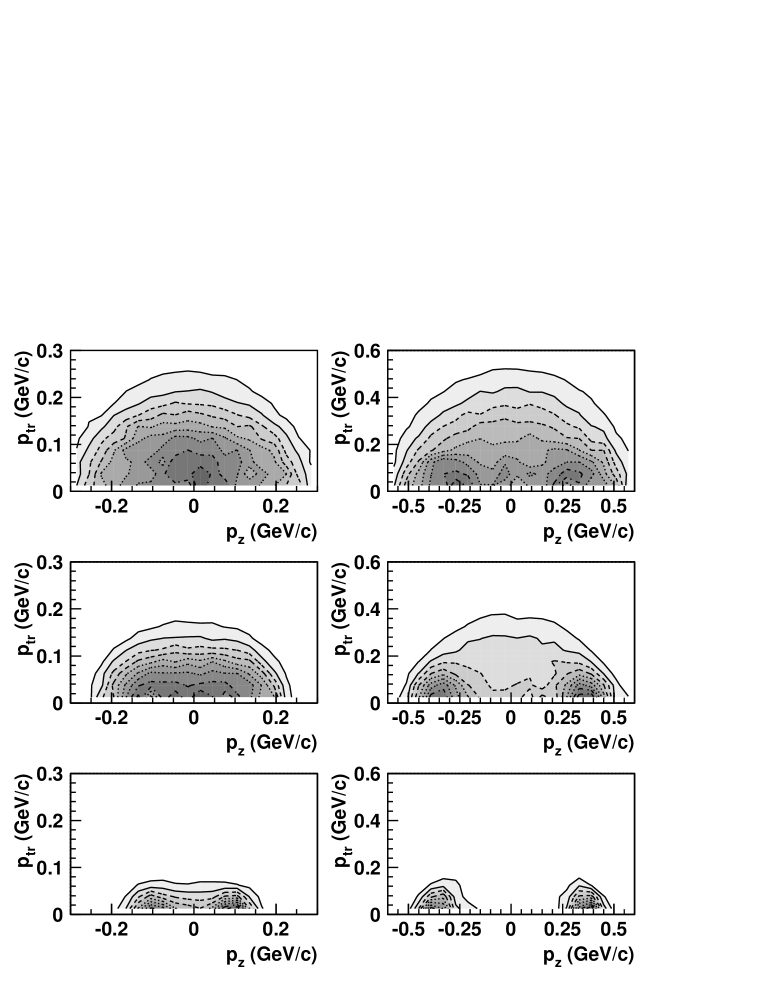
Figure 9: $\mbox{d}^{2}\sigma/p_{t}\mbox{d}p_{t}\mbox{d}p_{z}$ for A = 1 (top), $2\leq A\leq 4$ (middle) and $A\geq 5$ (bottom) produced in Xe + Sn, 50A MeV, 3 fm (left) and Au + Au, 400A MeV, 3 fm (right) reactions.

To get a better insight, we present (figure 9) the differential production spectra ($\mbox{d}^{2}\sigma/p_{t}\mbox{d}p_{t}\mbox{d}p_{z}$) of singles, light ($2\leq A\leq 4$), and heavy ($5\leq A$) fragments for Xe + Sn (50A MeV) and Au + Au (400A MeV) reactions at b = 3 fm . In this presentation, emission from a thermalized source produces circles of constant cross section around the source velocity.

At 50A MeV, the proton distribution is indeed nearly isotropic and could be attributed to a thermal source located at mid-rapidity. However, the light fragment distribution already contains a forward-backward enhancement which definitively evolves to a 2 sources emission-pattern for the heavy fragment production.

The situation at 400A MeV is somehow different: We observe 3 sources of protons that we naturally attribute to the mid-rapidity fireball, the projectile and the target remnants. For heavier fragments, the mid-rapidity source is weaker and the spectra more and more dominated by fragments emitted from projectile and target remnants. In other words, the importance of the mid-rapidity source decreases with the size of the fragment under consideration.

From figure 9, we can conjecture that for a given beam energy, the fragment distribution is always more anisotropic than the proton one. This clarifies the apparent paradox presented at the beginning of this section. This also implies that fragment spectra should be used preferably to proton ones for testing the degree of thermalization of any system.

In the framework of our model, b = 3 fm collisions never generate globally equilibrated nuclear matter. At high energy, it is a more or less a trivial consequence of the geometrical cuts encountered in the PS scenario, as mentioned previously. At low energy, another explanation has to be found. To disentangle the role of such cuts from other possible causes, we have analyzed the same reactions at b = 0 fm. At 400A MeV, distributions are close to isotropic whatever the class considered. This confirms that most of the anisotropy found at finite $b$ can be interpreted inside the PS scenario.

The situation is quite the opposite at 50A MeV. There, the distribution patterns found at b = 3 fm and b = 0 fm are basically identical. This observation definitively discards explanations exclusively based on some relative rotation (which would inhibit a complete fusion between the two partners, as it is invoked in the case of DIC scenario).

By now, we have accumulated enough insights to understand that at 50A MeV and small impact parameters, the majority of the projectile nucleons which are finally entrained in fragments have traversed the target (and vice versa). This is only possible because the Pauli principle blocks almost all collisions at this energy. Accordingly, the transparency anticipated at the end of section 3 indeed represents the mean behavior, and not a fluctuation on top of it.

Nevertheless, we must still reconcile this transparency hypothesis with the isotropy of the proton momentum-distribution. For this purpose, we use the following feed back argument: Initially, the system is both organized (nucleon-nucleon correlations) and anisotropic. We suggest that the nucleons finally emitted as singles are precisely the ones which have encountered the most violent/numerous collisions, necessary to destroy those correlations. Accordingly, their momentum distribution reaches a form compatible with a thermal spectra pretty fast. On the contrary, final fragments contain nucleons relatively unaffected by those collisions and of course maintain a memory of their initial momenta much longer.

The plausibility of this conjecture is checked in figure 10 where we have displayed, for the Xe + Sn (50A MeV, 3 fm) reactions, the mean number of collisions per nucleon as a function of time. We focus on those nucleons finally (a) emitted as singles, (b) members of $A\geq 5$ fragments. From figure 10, it appears that nucleons which turn out to be singles in the final stage have indeed undergone a higher number of collisions than those contained in fragments. For large times, the hadronic gas becomes more and more dilute, the single nucleons tend to evolve freely and the collision rate vanishes. On the other side, however isolated a fragment may be, its nucleons still collide with one another: This explains the constant collision rate ($\approx 1$ collision every 200 fm/c) observed asymptotically. These internal collisions do not modify the chemical composition in large respects. Those happening at early times are much more important because they determine the later composition. Then, to go beyond the qualitative picture, only the collisions happening during an effective reaction time of $\approx$ 80 fm/c should be taken into account. During this effective time, nucleons finally emitted as singles have collided roughly twice as much as nucleons emitted in heavy fragments… a spectacular difference! For the time, we do not pursue this analysis any further; we just retain the validity of our feed back argument and the incompatibility of results found in figure 10 with a global-equilibrium hypothesis.

In fact, the previous discussion is a perfect non-trivial example of time-correlation. It illustrates the power of these time-correlations in investigating the dynamics of nucleus-nucleus collisions. Later, in sections 5 and 6, we will study some of them more systematically. But first, we would like to conclude the topic of global equilibration by addressing it from another viewpoint: the mixing of projectile and target nucleons or, in other words, the “chemical” equilibration.

4.3 Equilibration according to the mixing of projectile and target nucleons

4.3.1 Motivation and redefinition of projectile/target-like and mid-rapidity fragments

We have already mentioned that PLFs, TLFs and MRFs may have a quite different origin. Accordingly, it is usually worthwhile to study these types of fragments separately, as we have already done in figure 7. For this purpose, it is very convenient to deal with a more practical (and maybe more general) criteria defining those classes. Such a criteria emerges naturally once we have realized that at high energy, PLFs (TLFs) are mainly composed of projectile (target) nucleons, while MRFs contain projectile and target nucleons with identical probability (for symmetric reactions).

Accordingly, from a theoretical point of view, we obtain more operational definitions of PLFs, TLFs and MRFs as following: we first remind the reader that $A_{p\,i}$ (resp. $A_{t\,i}$) has been defined as the number of nucleons initially contained in the projectile (resp. target) and finally emitted in the $i^{\mbox{th}}$ fragment. Next, we define

$$a_{i}=\frac{A_{p\,i}}{A_{p\,i}+A_{t\,i}}=\frac{A_{p\,i}}{A_{i}}$$ (17)

as the proportion of projectile nucleons in the $i^{\mbox{th}}$ fragment and classify the fragments according to their $a_{i}$:

$$\mbox{HF with}\hphantom{X}0.00\leq a_{i}<0.25 :$$ target-like-fragment (TLF)

$$0.25\leq a_{i}<0.75 :$$ mid-rapidity fragment (MRF)

$$0.75\leq a_{i}\leq 1.00 :$$ projectile-like-fragment (PLF) (18)

At high energy and finite impact parameter, both definitions coincide. Nevertheless, the definition given in formula 18 is more general (and will be adopted from now on), as it can also be used (see § below) to investigate chemical equilibration even in the absence of three sources clearly separated in rapidity, for instance at vanishing impact parameter or low energy. In fact, a detailed study of the rapidity distribution of TLFs, MRFs and PLFs has revealed that

$$y_{\mbox{targ}}\approx\overline{y_{TLF}}<\overline{y_{MRF}}<\overline{y_{PLF}}\approx y_{\mbox{proj}}\;,$$ (19)

whatever the energy and the impact parameter and however small $y_{\mbox{proj}}-y_{\mbox{targ}}$ may be. This explains why we stick to “mid-rapidity fragment” as a faithful label of the $0.25\leq a_{i}<0.75$ class, even if the new classification 18 does a priori not rely on any criteria involving the rapidity itself.

If the fragments are formed after the system has passed through a fully equilibrated phase, as it is expected in the compound nucleus scenario, we expect a distribution of $a_{i}$ according to a binomial law with a mean value of 0.5 (for symmetric reactions) and a variance inversely proportional to the square root of the fragment mass. Thus $a_{i}$ distribution should be sharply peaked around 0.5 for heavy fragments. On the other hand, in the simplest version of the PS model, we expect $a_{i}$ to be either 0 (TLF) or 1 (PLF). If participant and spectator matter interact weakly, we expect two narrow peaks around these values. What about the QMD results?

4.3.2 Distribution of projectile/target-like and mid-rapidity fragments

In figures 11 and 12, we present results of the model (A) for Au + Au, 400A MeV, 3 fm and Xe + Sn, 50A MeV, 3 fm reactions. In panel (a), we generalize the usual notion of mass spectrum $\mbox{d}\sigma/\mbox{d}A$: In fact, more detailed information is carried by the (normalized) double differential production cross section: $(\mbox{d}^{2}\sigma/\mbox{d}a\mbox{d}A)/(\mbox{d}\sigma/\mbox{d}A)$ . In panel (b), we present the differential cross-section for the production of HFs: $\left.\mbox{d}\sigma/\mbox{d}a\right|_{A\geq 5}$. This quantity is normalized to the total HF multiplicity. In panel (c), we plot the global mass spectrum, as well as the more specific mass spectra of P/TLFs and MRFs. Finally, in panel (d), the fragment-multiplicity distribution for IMFs ($5\leq A\leq 50$) and very heavy fragments (VHFs, $51\leq A$) are presented (see figures for more details).

We first discuss the high energy reactions. From the two upper panels of figure 11, we conclude that, independently of $A$, the overwhelming majority of fragments are either projectile-like or target-like: at 600 A MeV (not displayed), about 15% of the fragments are MRFs in nearly central collisions ($b_{<}$) and less than 1% in peripheral collisions ($b_{>}$). At 400A MeV these proportions increase to about 30% ($b_{<}$) and 4% ($b_{>}$).

Focusing on panel (c), we see that for high energy central collisions, the mass spectrum of MRFs and PLFs are almost identical in form—a power law. This is a remarkable result in view of the different production mechanisms. It confirms the conjecture that the mass spectrum is not very sensitive to the underlying physical process… a conclusion almost unavoidable if one remembers that the experimental mass spectrum is a pretty robust function of the system considered. Let us just mention that in high energy peripheral collisions, the MRF and P/TLF mass spectra naturally depart from one another: while no MRF of mass larger than 8 is found, the P/TLF spectrum extends up to A = 150, with a local minimum around A = 30-40.

From panel (d), we see that on the average 6 IMFs are produced (5 P/TLFs and 1 MRF), but no VHF. From the whole figure 11, one concludes that even though no heavy remnant is observed at such a low impact parameter, the memory of the entrance channel is fairly preserved. In the peripheral reaction already mentioned, two heavy remnants usually survive, in concordance with a “$<$” shape of the double differential cross section, but about 2 P/TLFs are produced as well.

In peripheral collisions, the typical behaviors observed at 50A MeV are pretty similar to those just discussed at 400A MeV (for $b_{>}$). Even though the total number of MRFs is larger at 50A MeV, it still does not represent more than 20% of all emitted HFs. As for the average fragment multiplicity, 2 VHFs survive the reaction and about 5 IMFs are produced (4 P/TLFs and 1 MRF) at low energy. In fact, the major discrepancy with the high energy case occurs in the study of the P/TLF and MRF mass spectra: these are now similar, up to A = 20. Also, P/TLFs of mass $A\approx 30-40$ are produced more abundantly and tend to fill the valley encountered at higher energy.

In low-energy central collisions (illustrated in figure 12), about 25% of all fragments are MRFs, while both mass spectra (MRF and P/TLF) are very close in form for almost all values of A. On the average, we do not observe two but only one remnant (VHF) which is either projectile or target-like, in definitive contradiction with a compound nucleus/incomplete fusion scenario. The disassembling of the other remnant is the basic cause of the broad mass-spectrum and the source of large fluctuations in the IMF yield.

By studying other energies between 400 and 50A MeV we have discovered nothing but a quite smooth crossover… and therefore established the generic character of figures 11 and 12, at least within the model (A)! By definition, results obtained in the two previous sections (4.1 and 4.2) are independent of the symmetrized character of the NN cross section. When we come to the question of chemical equilibration this is no longer the case. Accordingly, we have re-evaluated all quantities involved in figures 11 and 12 inside model (B) and re-displayed them in figures 13 and 14 respectively.

The most spectacular effect is observed for $\left.\mbox{d}\sigma/\mbox{d}a\right|_{A\geq 5}$ in panel (b): the peaks formerly observed around $a=0$ and 1 are now eroded, while at intermediate $a$, the valley is somewhat filled in… but we are still far from a dominating peak around $a=0.5$, as it would appear in case of chemical equilibration. In concordance with the flattening of $\left.\mbox{d}\sigma/\mbox{d}a\right|_{A\geq 5}$, one observes, in panel (d), an average increase (resp. decrease) of the MRF (resp. P/TLF) multiplicity by one unit. However, the VHF multiplicities are unaffected, as well as the general structure of the double differential cross section and the mass spectra (panels (a) and (c)).

On the qualitative level, we can conclude that chemical equilibration is achieved neither in model (A) nor in model (B), even if one gets closer with this second version of QMD.

To understand more quantitatively how the chemical equilibration depends on the model chosen and on the physical parameters (beam energy, impact parameter,…), we provide in table 2 the fraction of MRFs among HFs, for both models and various systems (those already chosen in table 1).

Within a wide range of physical parameters, the system is never close to chemical equilibrium; indeed, we observe very strong correlations between the origin of the particles (in this case projectile or target) and the type of fragment to which they will ultimately belong. In fact, the majority of fragments ”remain” projectile-like or target-like. Mid-rapidity fragments represent more than 40% of the yield only on a band located at high energy and low impact parameter.

In table 3, we provide a non-exhaustive list of qualitative dependences embedded in table 2. Let us comment on the third line and clarify the fifth one.

$\bullet$ Selecting b = 0 fm, and decreasing the beam energy, we expect to enter the realm of the quasi-fusion mode, where the proportion of MRFs should in principle re-increase. At 50A MeV, this is not yet the case.

$\bullet$ Whatever the system, the energy and the impact parameter, it turns out that the MRF yield inside model (B) is approximatively $3/2$ of the MRF yield inside model (A):

$$\sigma_{prod}(MRF)|_{\theta_{cm}\leq\pi}\approx\frac{3}{2}\sigma_{prod}(MRF)|_{\theta_{cm}\leq\frac{\pi}{2}}\;!$$ (20)

Of course, this result cannot be universal: a priori, there must exist an energy for which a nucleus-nucleus collision happening at b = 0 fm engenders a highly equilibrated phase, whatever the model chosen. However, in the energy range relevant for (multi)fragmentation, this is not the case, and relation 20 seems to hold. We propose the following interpretation: at the early stages of a reaction or in case of a poor equilibration, the production of chemically-equilibrated matter is proportional to the rate of projectile nucleons deflected in the phase space of target nucleons (plus a symmetric contribution). This deflection rate itself is proportional to the collision rate multiplied by the mean deflecting angle associated with the microscopic interaction, defined as

$$\bar{\theta}_{deflect}=\mbox{arccos}\left[\int\cos\theta\frac{1}{\sigma}\frac{\partial\sigma}{\partial\Omega}\mbox{d}\Omega\right]$$ (21)

Precisely, what distinguishes model (A) from model (B) is just that interaction. At low energy,

$$\frac{\partial\sigma}{\partial\Omega} = \frac{\sigma_{NN}}{2\pi}\hphantom{0}\mbox{for $\theta\in[0,\frac{\pi}{2}]$}$$

$$0\hphantom{\frac{\sigma_{NN}}{2\pi}}\mbox{for $\theta\in]\frac{\pi}{2},\pi]$}$$

in model (A) and

$$\frac{\partial\sigma}{\partial\Omega} = \frac{\sigma_{NN}}{4\pi}\hphantom{0}\mbox{for $\theta\in[0,\pi]$}\;.$$ (22)

in model (B). Accordingly,

$$\bar{\theta}_{deflectA}(E\ll)\approx\frac{\pi}{3}\mbox{ and }\bar{\theta}_{deflectB}(E\ll)\approx\frac{\pi}{2}\;.$$ (23)

In the linear approximation, this permits to reproduce relation 20. If the linear approximation breaks down, the ratio $\theta_{deflectB}/\theta_{deflectA}=\frac{3}{2}$ probably acts as a scaling factor. From this analysis, we conjecture that, quite generally, using model (B) instead of model (A) reduces the amplitude of time-correlations by a mere factor, but does not destroy them dramatically, as it could have been feared a priori. In the last analysis, this would not be so surprising: The (chemical) relaxation times of model (A) and (B) seem to differ by just a factor $\approx 1.5$! If global equilibration were achieved in one of them, it would be automatically achieved in the other. In other words, to choose one model or the other would result in the same qualitative understanding of the underlying physics, which is, after all, the main goal of this work.

We now close this whole section devoted to the question of global equilibration. In fact, table 1 and table 2 reflect two aspects of this problem: the equilibration of the momentum distribution and the chemical equilibration… They exhibit the same qualitative dependences on the physical parameters and lead to the same conclusion: For the impact parameters and energy range (50-600A MeV) investigated in QMD simulations, the system only approaches global equilibrium on a domain located at very high beam energy and very small impact parameter… a range of no interest for multifragmentation.

5 Initial-final state correlations

In this section, we search for the possible phase-space correlations between the initial and the final state of our simulations. To be more specific, we would like to know whether nucleons finally entrained in fragments were predominantly located in certain regions of phase-space at the initial time. We shall proceed in several steps.

After detailing the actual way those time-correlations were evaluated (section 5.1), we investigate separately the case of light fragments or singles (LF) and of heavy fragments (HF) in the coordinate space (section 5.2). Later (section 5.3), we refine the HF analysis by focusing on the mid-rapidity fragments and the projectile/target-like fragments.

In a second step, we perform the equivalent study in the momentum space (sections 5.4 and 5.5). This will help us to understand better the question of longitudinal correlation, left open up to there. In section 5.6, this problem will clarified by introducing the concept of “catapult mechanism”.

5.1 Evaluation of the time-correlations

For instance, suppose we want to know from which part of the initial (one-body) phase-space stem the nucleons found in final fragments. In the QMD model, this can be done via the following procedure:

• store the initial positions $r_{i}(t=0)$ and momenta $p_{i}(t=0)$ of all $A_{P}+A_{T}$ nucleons;

• simulate the reaction up to $t_{fin}$ (i.e. 180 fm/c);

• perform clusterization at $t_{fin}$ using a minimum spanning-tree algorithm with a given clusterization radius (i.e. 4 fm);

• define $inclass_{i}=1$ if at $t_{fin}$ the nucleon i is part of a fragment belonging to the class to investigate. Otherwise $inclass_{i}=0$

• project the initial positions $r_{i}(t=0)$ on a 2 dimensional grid. Each vector $r_{i}(t=0)$ now corresponds to a grid cell k.

• define 2 quantities $\rho_{class,k}=\sum inclass_{i}$ and $\rho_{tot,k}=\sum 1$ where the sum runs over all nucleons whose coordinate vector falls into the grid cell k

• perform the mean of $\rho$’s on an ensemble of simulations

• display the quantities $\rho_{class,k}$ and $\hat{\rho}_{class,k}=\rho_{class,k}/\rho_{tot,k}$.

In case of global equilibration, correlations between initial and final states are absent and nucleons emerge equiprobably from the initial phase space. It results that $\hat{\rho}_{class,k}$ is constant (i.e. independent of $k$), whatever the class. On the other hand, in the PS scenario, $\hat{\rho}_{HF,k}$ is close to 1 outside the geometrical overlap and close to 0 otherwise. Of course, the actual physical processes turn out to be more subtle than those two idealized pictures, as we will now discuss.

5.2 Coordinate-space correlations of light and heavy fragments.

5.2.1 Energy dependence

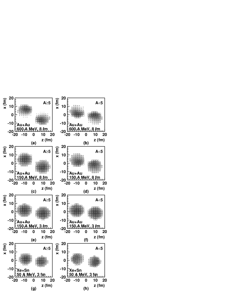
Figure 15: Initial-final state correlations in coordinate space: On the left (resp. right), initial densities of nucleons finally entrained in $A\geq 5$ (resp. $A<5$) fragments. The shading represents those absolute densities , while the area of the boxes represents their local ratio with the total density of nucleons. From top to bottom: (Au + Au, 600A MeV, 8 fm), (Au + Au, 150A MeV, 8 fm), (Au + Au, 150A MeV, 3 fm) and (Xe + Sn, 50A MeV, 3 fm).

We start the analysis of initial-final state correlations focusing on the coordinate space. The left panels of figure 15 illustrate these correlations for nucleons finally entrained in HFs, for several systems: from top to bottom: (Au + Au, 600A MeV, 8 fm), (Au + Au, 150A MeV, 8 fm), (Au + Au, 150A MeV, 3 fm) and (Xe + Sn, 50A MeV, 3 fm). The shadings correspond to $\rho_{HF,k}$, whereas the boxes size represents $\hat{\rho}_{HF,k}$. Both quantities are normalized relatively to the grid cell containing the largest value. The right panels are just the counterpart for the LF case.

At high energy, the PS model should apply. As a matter of fact, in panels (a) and (b), we observe that HF nucleons come predominantly from the spectator regions, while LF ones, from the participant zone. The transition from the “participants” to “spectators” is quite clear but not as sharp as in the PS model itself. This is not the only difference: A closer look at panels (a) and (b) reveals that the transverse extent of the “participants” and “spectators” zones depends on z. This longitudinal dependence is absent of the PS model and we conjecture that it reflects the expansion of the fireball already formed by the participants on the front of the nuclei. Due to high temperature, these nucleons disassemble very quickly (before the projectile and target back ends arrive at the interaction zone) penetrate the incoming spectator matter and excite it locally (within a mean free path distance). As a direct consequence, this excited spectator matter will form more LFs and less HFs.

At lower beam energy, we observe a gradual disappearance of the correlations predicted by the PS model. Already at 400A MeV (not displayed), the correlations are weakened. Between 400A MeV and 50A MeV, the reaction mechanisms change completely. At 150A MeV, 8 fm, we observe some spatial correlation only in the distribution of nucleons emerging as LF (panel (d)). For an impact parameter of 3 fm, almost no correlation is seen, as it would happen if the system were completely equilibrated. However, we have already seen in section 4 that this hypothesis is not correct.

For nearly central collisions at 50A MeV, we observe correlations along the beam axis. Nucleons at the back ends of projectile and target have a higher probability to form a light fragment or to escape as singles than those at the front end. With the data at hand, it is not possible to interpret this result unambiguously. One could think that the two nuclei rotate around each other. Both front ends would fuse in this rotation, while the back ends would be ejected by the centrifugal force… however, we have already seen (see for instance section 3 and more precisely figure 7) that the rotational character is rather small at this impact parameter. In fact, what is really happening is totally different: In section 5.6, we will explore other time-correlations and demonstrate that the dense zone formed in the projectile-target overlapping region acts as a catapult for the nucleons which are initially at the back ends of projectile and target. These nucleons are accelerated mostly expelled as singles.

Summarizing, we see a complete change of the coordinate-space correlations pattern if we decrease the energy from 600A MeV to 50A MeV.

5.2.2 Quantification of the correlations

To facilitate the comparison between different energies, impact parameters, etc., it is helpful to define a single numerical quantity reflecting the importance of the initial-final state correlations. For light fragments, we have found appropriate to define the “coordinate space LF correlation number” as follows:

$$C^{r}_{LF}=\frac{\sqrt{\overline{\left(\hat{\rho}_{LF}-\overline{\hat{\rho}_{LF}}\right)^{2}}^{\vphantom{l}}}}{\overline{\hat{\rho}_{LF}}}\mbox{, with }\hat{\rho}_{LF,k}=\frac{\rho_{LF,k}}{\rho_{tot,k}}\;,$$ (24)

where $\rho_{LF}$ is the initial density of nucleons emerging asymptotically as light fragments and $\rho_{tot}$ is the mean density in initial nuclei. Here, “$\overline{\vphantom{x}...}$” represents the average taken on all cells $k$ such that $\rho_{tot,k}\geq\mbox{max}(\rho_{tot})/10$. This condition is set to discard the unphysical fluctuations in the low density regions. We define $C^{r}_{HF}$, the “coordinate space HF correlation number”, in a quite similar way. As $\hat{\rho}_{LF}\leq 1$, we easily establish that

$$C^{r}_{LF}\leq\sqrt{\overline{\hat{\rho}_{LF}}^{~{}-1}-1},$$ (25)

(and similarly for $C^{r}_{HF}$), indicating that correlations are intrinsically limited if a large number of nucleons are requested in a given final channel (as a limit, they vanish if all the nucleons are needed). This is for instance the case for the production of LF in high-energy central collisions. Moreover, as $\hat{\rho}_{LF}+\hat{\rho}_{HF}=1$, one has

$$\overline{\hat{\rho}_{LF}}*C^{r}_{LF}=\overline{\hat{\rho}_{HF}}*C^{r}_{HF}$$ (26)

and of course

$$\overline{\hat{\rho}_{LF}}+\overline{\hat{\rho}_{HF}}=1\;.$$ (27)

In table 4 we summarize the values of $\overline{\hat{\rho}_{LF}}$ and $\overline{\hat{\rho}_{HF}}$ for Au + Au (600, 400 and 150A MeV) and Xe + Sn (50A MeV) reactions, at small ($b_{<}$) and large ($b_{>}$) impact parameter. In table 5, we summarize the values of $C^{r}_{LF}$ and $C^{r}_{HF}$ for the same reactions. In high-energy central collisions, one obtains a large number of nucleons going to LFs and, according to relation 25, a low value of the correlation number. In all other high energy reactions and fragment classes, strong correlations are present, in agreement with the PS model.

When the energy decreases, more and more nucleons are released in HFs and the associated correlation numbers vanish… once again a consequence of inequality 25! In fact, at low energy, one intuitively expects a transition into the direction of a compound-nucleus reaction. This would imply a complete mixing of all nucleons and the disappearance of all initial-final state correlations. However, this is clearly not observed: At large impact parameter ($b_{>}$), the correlations in $\rho_{LF}$ survive, while for central collisions ($b_{<}$), they even increase as compared to the high energy case.

From table 5 it also appears that when the energy is reduced, the quantities at hand (here, the correlation number) depend on the impact parameter in a much smoother way; a fact already observed many times, for instance in table 1.

5.3 Coordinate-space correlations of projectile/target-like and mid-rapidity fragments

We start the comparison by extracting, in table 6, $\overline{\hat{\rho}_{MRF}}$ and $\overline{\hat{\rho}_{P\cup LF}}$ for a few systems and both models (but we first concentrate our discussion on model (A)).

Table 6 confirms that the PLFs and TLFs outnumber the MRFs at all energies, but this is especially true for high energy and high impact parameter. $C^{r}_{MRF}$ and $C^{r}_{P\cup TLF}$ are defined as $C^{r}_{HF}$, but with the proper selection on the fragment type. These correlations numbers are displayed in table 7.

Due to the dominance of PLF and TLF channels, $C^{r}_{P\cup TLF}$ and $C^{r}_{HF}$ are pretty close (cf. table 5). More astonishing are the strong correlations exhibited in the MRF channel. These are the strongest correlations observed so far. In central collisions, they even increase when energy is reduced.

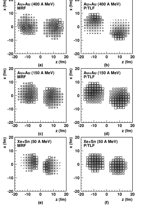
Figure 16: Coordinate-space initial-final state correlations: initial density of nucleons entrained finally in heavy fragments $(A\geq 5)$, separately for MRF (left) and P/TLF (right). Three cases of central (b = 3 fm) collisions have been considered: Au + Au, 400A MeV (top), Au + Au, 150A MeV (middle) and Xe + Sn, 50A MeV (bottom).

To investigate the nature of these correlations in more details, we display in figure 16 the coordinate-space correlations in the b = 3 fm reactions computed in model (A), following the conventions of figure 15. Correlations for MRFs and P/TLFs are shown on the left and right side respectively.

At 400A MeV, MRFs’ nucleons are initially located in the “participant” zones, while the PLFs and TLFs’ nucleons are found in the “spectator” zones. These zones are clearly separated: participant nucleons penetrate the spectator matter only occasionally, so that its composition is basically unchanged. On the other hand, they create and enter a “fireball” which emits a few MRFs in a much more statistical way.

At 150A MeV, the PS model does not apply anymore and the transverse correlations associated with it have indeed completely disappeared. This break down (of the transverse time-correlations) was first mentioned in section 5.2 by the inspection of figure 15. From the panel (e) of this figure, one could have been tempted to conclude the absence of (coordinate-space) time-correlations in the HF formation process at 150A MeV. However, the refined analysis performed in figure 16 reveals that the HF fluid is in fact made of three components (MRF, PLF and TLF), each of these exhibiting strong time-correlations. This behavior is even more pronounced at 50A MeV, where the nucleons finally entrained in MRFs are strongly localized along the longitudinal axis. Why longitudinal? We do not have enough information to answer this question right now and leave it open until section 5.6.

How do the results of model (B) match those of model (A)? Inspecting table 7, MRF correlation numbers turn out to be reduced by 33% on the average and by 50% at the most (for 150A MeV). PLF correlation numbers are basically left untouched, whatever the physical parameters. Even if not displayed here for the purpose of concision, let us stress that when correlations illustrated in figure 16 are re-evaluated inside model (B), they present exactly the same characteristic pattern, slightly attenuated.

5.4 Momentum-space correlations of light and heavy fragments

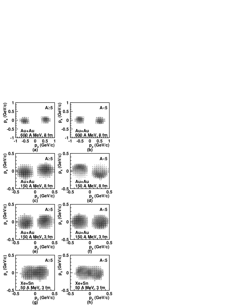
Figure 17: Momentum-space initial-final state correlations: initial density of nucleons entrained finally in heavy fragments have been plotted for the same reactions as in figure 15.

Usually, correlations between the initial momentum of the nucleons and their probability to end up in a given type of cluster are not considered as important. In general, phenomenological models assume that there are no such correlations. However, the QMD calculations show quite strong correlations. In figure 17, we present these correlations in momentum space, in the same way as we did for the coordinate space in figure 15.

At 600A MeV we see that the heavy fragments are formed from nucleons which have a momentum pointing away from the collision partner. This qualitative observation is independent of the impact parameter but the correlations are quantitatively stronger at smaller impact parameter (cf. table 8). At lower energy the correlation in $x$ direction is weakened and starting from E = 150A MeV supplemented by correlations in $z$ direction, especially important for the LFs.

While it is pretty easy to understand the origin of the transverse correlations at high energy, the longitudinal ones observed at low energy are more subtle to grasp. They rely on two points:

• One needs efficient collisions to produce light fragments quickly (this can be seen at the best on figure 10).

• At low beam energy, the Pauli blocking of the cross section is quite strong, but less drastic for nucleons incoming with higher relative momentum. In other words, nucleons helped coherently by the Fermi momentum have a higher probability to scatter into an empty place of phase space.

Combining these two points, one concludes that nucleons entering the reaction zone with large $|p_{z}|$ are more likely to end up in a light fragment than the others. At E = 50A MeV the Pauli blocking is severe: For almost all momenta one can reach in a nucleon-nucleon collision, the phase space cells are already occupied. Hence, the phase space opens up only for those nucleons incoming with particularly large values of $|p_{z}|$.

To quantify the correlations in momentum space, we define the correlation numbers $C_{LF}^{p}$ and $C_{HF}^{p}$, exactly as we did in section 5.2 for the correlations in coordinate space. In table 8, we display some values of $C_{LF}^{p}$ and $C_{HF}^{p}$.

In general, the correlations in r and p-spaces are of the same order. In fact, r-space correlations are larger than p-space ones at high energies and smaller at low energies.

5.5 Momentum-space correlations of projectile/target-like and mid-rapidity fragments

The correlation numbers in momentum space are presented in table 9.

As in coordinate space, strong correlations are observed, especially for the MRFs, which are essentially composed of participant nucleons (cf. section 5.3). Consequently, we conclude that the participants do not really form a fireball (defined as an equilibrated system resulting from the destruction of all initial correlations).

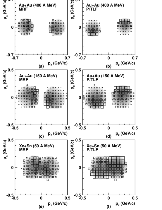
Figure 18: Momentum-space initial-final state correlations: initial density of nucleons entrained finally in heavy fragments $(A\geq 5)$, separately for MRF and P/TLF. The same reactions as in figure 16 have been studied.

In figure 18, we illustrate the momentum-space time-correlations both for MRFs and P/TLFs. P/TLFs mainly contain nucleons with an initial momentum pointing away from the collision partner. This type of correlation was already discovered in section 5.4, in analyzing the HF’s case.

On the other hand, correlations of MRF’s nucleons differ completely: Independently of the beam energy, MRFs are predominantly formed by nucleons which had initially a small energy in the nucleus-nucleus center of mass. As a matter of fact, nucleons with higher relative momentum possess a higher chance to perform a collision, due to their larger open phase space. Collisions provide a large momentum transfer and lower the probability to find several fellow nucleons with about the same final momentum, a necessary environment to form a fragment. Moreover, because of the relatively poor stopping at low energy, nucleons are only afforded a brief amount of time, during which they have to mix… if a MRF should be emitted. This constrain also favors nucleons with small relative energy, which have the possibility to stay longer in contact.

Finally, we note that, as previously, we do not see any dramatic reduction or modification of the correlations when the model (B) is used instead of the model(A): From now on, we shall confidently restrict ourselves to the model (A).

5.6 Catapult mechanism at low energy

We shall now exploit the knowledge just gained about the longitudinal correlations in p-space at low energy to understand those in r-space.

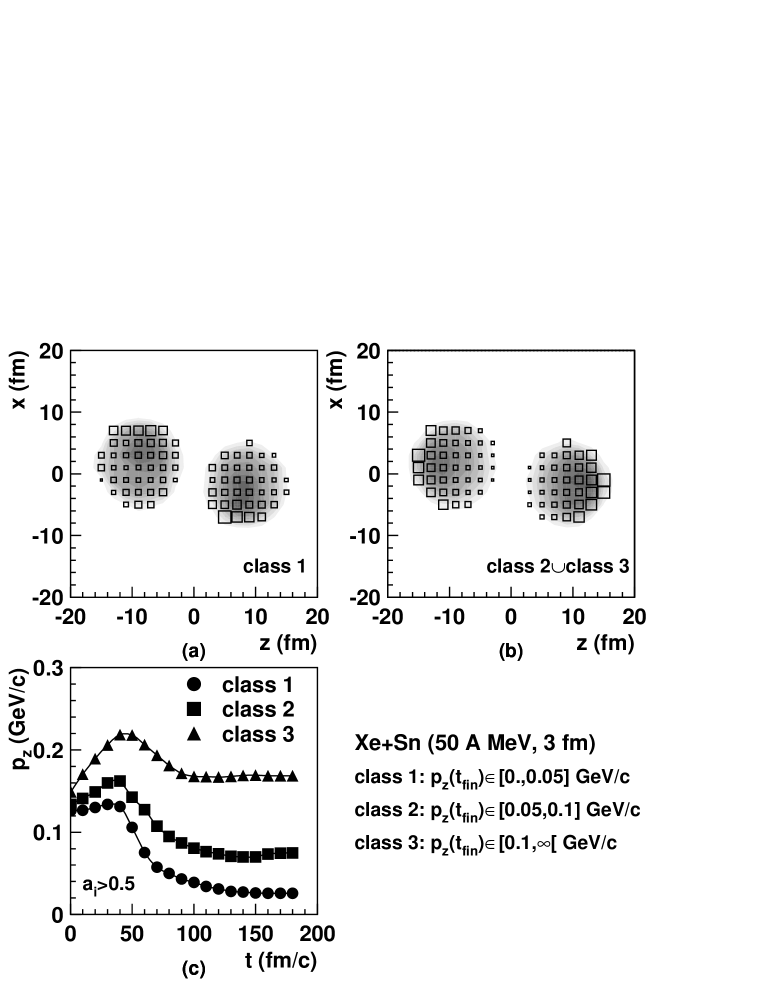
Figure 19: Xe + Sn reaction at E = 50A MeV, b = 3 fm: initial position of those nucleons finally emitted in light fragments $(A\leq 4)$ with (a) a small (b) large absolute longitudinal momentum per nucleon. We also display (c) the time evolution of the longitudinal momentum for three classes of nucleons.

In fact, such longitudinal correlations are not completely new to the expert: a while ago it has already been observed that the most energetic nucleons appear in the half-plane opposite to the impact parameter [31]. This is surprising, because these nucleons have to cross the entire nuclear system. To investigate the origin of this intriguing process we have selected, for the 50A MeV reaction, nucleons which have finally the highest longitudinal momentum and searched for their initial position and momentum. Results are presented in figure 19.

The particles with a moderate final momentum come from the participant zone, whereas the most energetic nucleons come from the back ends of the colliding nuclei, in agreement with [31]. Initially these nucleons are not faster than their fellow nucleons, but when they pass through the nucleus they get accelerated (cf panel(c)). Only later, when they have to overcome the nuclear potential they loose momentum.

We suggest the following reason: on the average, nucleons located at the back end surface of the projectile at initial time become the fastest ones some tens of fm/c later. One can then apply the arguments developed in section 5.4, where we have discussed in details why fast nucleons should emerge more easily as singles in low-energy reactions.

Let us now clarify the physical mechanism: In a nucleus, nucleons are continuously moving and accelerated. At a given time, nucleons located at the surface feel a density $\rho<\rho_{0}$ and are nearly at rest, as they have given their kinetic energy to climb the mean-field potential. Later on, strongly re-accelerated towards the nucleus center by the force due to the density gradient, they become the fastest ones. Usually, they pass the center, arrive at the other end of the nucleus and are stopped again…If a 50A MeV reaction takes place in between, the first stages of this scenario are basically unchanged: at low beam energy, the density increases very little in the interaction region and remains almost constant until the nucleons have passed the entire reaction partner. At this time, they should normally be stopped. However, the relative momentum between them and the nucleons at the end of the reaction partner has now increased by the beam momentum and the density gradient decreased, due to dilution of nuclear-matter. As a result, the force at the surface is no longer sufficient to stop those fast nucleons and they are just decelerated (see figure 19).

This catapult mechanism also explains the longitudinal correlations observed in the MRF channel. Nucleons initially at the front end of the projectile are accelerated in the direction opposite to the beam momentum. Very soon, they become the slowest ones in the system, what increases their probability to emerge in MRFs, as demonstrated in section 5.5.

5.7 Summary of the phase-space correlations

Up to now we have investigated the existence of possible correlations between the initial position of nucleons in r and p-space and their final fate. Table 10 summarizes our present findings concerning the correlations.

It turns out that there are two rather distinct classes of heavy fragments: those which are formed almost exclusively by projectile or target nucleons and those which are close to chemical equilibrium. For both classes we observe strong initial-final state correlations, however different in their nature. At high energy, we recover the PS model and its associated transverse correlations in coordinate space with, nevertheless, strong supplementary correlations in momentum space.

At lower energies, a semi-transparent regime was established: The PLFs (resp. TLFs) are mostly formed by nucleons which have traversed the entire target (resp. projectile). Due to the severe Pauli blocking of the collisions, projectile nucleons can indeed keep their correlations while traversing the target and vice versa. On the top of this mean behavior, longitudinal correlations in r and p-space were also discovered. For instance, it appeared that MRF are formed preferably by nucleons having a very small energy in the nucleus-nucleus center of mass. In section 6, we investigate further those reaction mechanisms.

Before this, we would like to interpret the 600A MeV results in view of the dependence of the transverse flow on the fragment mass. Already the plastic ball collaboration has observed [28] that the directed transverse flow increases as a function of the mass number.

In section 5.2, we have found that the large fragments (even in central collisions) are made of spectator nucleons. They do not pass a region of high density. Thus the directed transverse flow does not measure properties of the high density zone but the gradient of the potential at its surface. Therefore the flow can only measure the high density properties of nuclear matter which can be inferred from the gradient of the potential at the surface of the high density zone!

In section 5.4, the situation was found to be even worse. Indeed, the average initial transverse momentum of the fragment’s nucleons differs from zero. This means that the above-mentioned transverse flow is partially generated during the collisions but also results from initial-final state correlations. This questions another time the value of the observable flow as a messenger of the properties of the high density zone.

These findings must be confronted with the recent observation that the strange particle production at that energy takes place in the high density region [17]. Therefore these particles provide a more direct information about the high density zone.

6 Time evolution of the reaction

Now we have examined initial properties of the nucleons related to the nature of the produced fragments, we turn to the time-dependence of another set of observables, in order to understand better how those fragments emerge from the reaction. A typical point we would like to clarify is how close the nucleons finally forming a fragment have been in the past. Does a nucleus-nucleus collision resemble a stone-stone collision? Or is it more an evaporation-recondensation mechanism? Besides, we would like to understand how a typical prefragment evolves under its interaction with the “external” nucleons (defined as all the $A_{P}+A_{T}-A$ nucleons which do not belong to the same prefragment).

6.1 Radii and densities

In relation 14, we have defined the center of mass ($\vec{R}$) and the mean momentum per nucleon ($\vec{P}$) of a given prefragment. In the same spirit, we define for our purpose:

• $Rad(t)$, the radius of the prefragment as

  $$Rad(t)=\sqrt{\frac{\sum_{i=1}^{A}(\vec{r}_{i}(t)-\vec{R}(t))^{2}}{A}}$$ (28)

• $Rad_{\perp}(t)$, the normalized transverse radius of the prefragment as

  $$Rad_{\perp}(t)=\sqrt{\frac{3}{2}\frac{\sum_{i=1}^{A}(\vec{r}_{i,\perp}(t)-\vec{R}_{\perp}(t))^{2}}{A}}\;,$$ (29)

  where the $\perp$ suffix indicates a transverse projection. The $3/2$ normalization factor allows a direct comparison with values of $Rad$.

• $\rho_{int}(t)$, the density of the prefragment matter at its own center of mass as

  $$\rho_{int}(t)\ \propto\sum_{i=1}^{A}e^{-\frac{(\vec{r}_{i}(t)-\vec{R}(t))^{2}}{2\rho_{0}^{2}}}$$ (30)

• $\rho_{ext}(t)$, the mean density of “external” matter at the center of mass of the prefragment as

  $$\rho_{ext}(t)\ \propto\sum_{i=A+1}^{A_{P}+A_{T}}e^{-\frac{(\vec{r}_{i}(t)-\vec{R}(t))^{2}}{2\rho_{0}^{2}}}\;,$$ (31)

  where the sum runs on all external nucleons. In fact, the small value of $2\rho_{0}^{2}$ (2.17 $\mbox{fm}^{2}$) automatically favors external nucleons close to $\vec{R}$, without any supplementary condition.

One has of course

$$\rho(\vec{R}(t),t)=\rho_{ext}(t)+\rho_{int}(t)$$ (32)

but one will see that the distinction between internal and external matter is quite fruitful. As usual, we average on all fragments of a given class and on a significant ensemble of QMD runs.

On figure 20, we plot the time evolution of these newly defined coordinate-space variables for b = 3 fm reactions (radii at the top and densities in the middle). We address the case of MRF in Au + Au (400A MeV), as well as MRF and PLF in Xe+Sn (50A MeV), from left to right.

We mark with a plain arrow the initial value expected if no correlation were present, i.e. if fragments were made by taking nucleons randomly from projectile and target, but in the proper composition ($a_{i}$). Hence differences between plain arrows and actual values are due to the nonuniform distribution (over the target and projectile) of prefragment nucleons at initial time. This is nothing but the initial-final state correlations already discussed.

For 400A MeV there is no correlation in longitudinal direction but a small one in transverse direction. MRFs stem to a large extent from the participant region which has a smaller transverse size than the combined system of participants and spectators. If we go down to the lower energy we observe initial correlations also in longitudinal direction as already seen in figure 15 and 16.

The dashed arrow marks the initial value expected if one takes the nucleons (in the proper composition ($a_{i}$)) randomly from a one-body distribution made of all nucleons belonging to the same class of prefragments (MRF or PLF). Any difference between the dashed arrow and the actual value gives a new insight: it indicates the presence of true many-body correlations, for example that fragment nucleons have been already close (in coordinate space) initially.

Introducing this refinement, we see that part of the discrepancies between the pure statistical model (plain arrows) and the actual values can be understood in terms of one-body effects (dashed arrows), but only part of it, pleading for some many-body correlations.

Let us examine the time-evolution: at 400A MeV, it takes about 30 fm/c—50 fm/c at 50A MeV—until the transverse and the longitudinal sizes of the prefragment match. In fact, the radii decrease while nucleons from different regions of projectile and target join to form a fragment (the higher the energy the smaller is the probability for the prefragment nucleons to have been already close together initially). One can conclude that those coordinate-space correlations are one but not the essential reason for fragment formation.

This is even better reflected by the increase of the prefragment internal density: at small times $\rho_{int}$ is still quite low and strongly dominated by $\rho_{ext}$, even at the center of mass of the prefragment itself. Let us also notice that for the 400A MeV reaction, $\rho_{ext}$ exceeds by far the normal nuclear-matter density.

After 100 fm/c (for the 400A MeV reaction) or 150 fm/c (for the 50A MeV reaction), no other nucleon can be found around the prefragment’s members. At that time the prefragments have separated from each other and can be considered as real and dense fragments, easily identified by a minimum spanning tree algorithm.

From the reactions we have studied in this section, one can conclude that nucleus-nucleus and stone-stone collisions have little in common, at least as far as the mechanisms for fragment formation are concerned. In the next section, we demonstrate that an evaporation-recondensation scenario is irrelevant as well.

6.2 $P_{z}$ and effective temperatures

In a dedicated study, it appeared that at low energy (50A MeV), $\overline{P_{z}}$, does practically not change in the course of time. At higher energy, this statement has to be attenuated, but is still relevant at 400A MeV… Is it really so that the average prefragment passes through the high density/temperature zone without being affected by it? To obtain new insights into this question, a natural way consists in comparing their respective temperatures (or excitation energies). For this purpose, we introduce:

• $T_{int}(t)$, the effective temperature of the prefragment as

  $$T_{int}(t)=\frac{\sum_{i=1}^{A}(\vec{p}_{i}(t)-\vec{P}(t))^{2}}{3.m_{N}.A}$$ (33)

  where $m_{N}$ is the nucleon mass. Note that $T_{int}(t)$ is an effective temperature of the fragment which agrees with the true temperature only in the case of a Maxwellian momentum-distribution. However, being the second moment of the momentum distribution it gives, in any case, a measure for the excitation energy/nucleon.

• $T_{\perp~{}int}(t)$, the effective transverse temperature of the prefragment, defined as above by taking only into account the transverse degrees of freedom.

• $\vec{P}_{ext}(t)$, the mean momentum of the external matter as

  $$\vec{P}_{ext}(t)=\frac{\sum_{i=1}^{A_{ext}(t)}\vec{p}_{i}(t)}{A_{ext}(t)}\;,$$ (34)

  where $A_{ext}(t)$ is the number of external nucleons located within 3 fm from the prefragment center of mass $\vec{R}(t)$.

• $T_{ext}(t)$, the effective temperature of the external matter as

  $$T_{ext}(t)=\frac{\sum_{i=1}^{A_{ext}(t)}(\vec{p}_{i}(t)-\vec{P}_{ext}(t))^{2}}{3.m_{N}.A_{ext}(t)}$$ (35)

  where the sum over i is performed on the same nucleons as for $\vec{P}_{ext}(t)$. Again, this quantity is to be considered as a probe of the medium excitation-energy.

• $T_{\perp~{}ext}(t)$, the effective transverse temperature of the external matter, i.e. the second moment of the momentum distribution in transverse direction.

As usual, the double averaging is performed. At the bottom of figure 20, these various temperatures are displayed for the same reactions as those considered in section 6.1

The external temperatures show the expected behavior: When projectile and target nucleons interact, the system heats up and the variance of the momentum distribution increases. In an equilibrated system, the transverse and total temperature should be equal. This is definitively not the case in our results, until 40 fm/c for the 400A MeV reaction and until 90 fm/c for the 50A MeV reaction. This lack of external equilibrium is consistent with all the correlations found so far. Finally the temperature lowers because the system disassembles and—depending of their velocity—the external nucleons leave the 3 fm sphere around the moving center of mass of the prefragment. Now, only prefragment nucleons are present in this sphere and therefore the external variances become identically zero.

The internal temperatures show a completely different behavior: Initially the prefragment nucleons have a lower variance than expected from a random selection of those nucleons. As expected, MRF nucleons have a quite large variance in the beam direction. In the course of the time, the internal temperatures decrease even before the system expands. This behavior completely contradicts our intuition as well as our experience from thermodynamics. In a thermodynamical language: the fragments cool down by giving energy to the already hot environment. It is obvious that these findings forbid to consider the second moment as a common temperature, in the sense of Gibbs’ criteria: $T_{int}=T_{ext}$.

To understand what is actually happening, one uses—once again—a feedback argument: In the end, only those nucleons with small relative momenta form clusters. In the course of the reaction, it happens that some nucleons are scattered into the vicinity (in phase space) of one nucleon or a cluster of nucleons. With respect to these nucleons the variance of the relative momentum is smaller after the collision than before. If the nucleons do not scatter once more they may leave the interaction region as a group and may form a cluster. If a nucleon scatters once more it will not be entrained in this cluster and hence will not affect the evaluation of $T_{int}$.

Thus one may conclude that:

• Initial correlations are present: Geometry and relative momenta determine how probably nucleons are scattered out of or into certain momentum-space regions.

• Although located at the same place in coordinate space as the surrounding nucleons, the prefragment nucleons have a much lower variance of their relative momenta. The fragment formation is hence a fluctuation on the level of the one-body phase space distribution.

• Fragments are formed (a) by nucleons which are already close in phase space at the beginning of the reaction and keep this correlation during the reaction and (b) by nucleons which are brought by accident into the same phase space region (this may be a consequence of two-body scattering or of the potential interaction for MRF). In other words, fragmentation is a mixture of conserving initial correlations (for projectile and target-like fragments) and of building up new correlations in the course of the interaction (for mid-rapidity fragments).

7 Conclusions

Using the QMD model, we have extensively studied the process of multifragmentation in heavy ion induced reactions. We have validated the QMD approach by showing that the presently available data are in even better agreement with the calculation than expected in view of approximations made in the model, especially at low energy. Also, we have checked and explained in details that the qualitative conclusions given hereafter depend very little on the symmetrized character of the microscopic NN interaction.

At all energies, we have found that correlations in coordinate and momentum space (the memory of the entrance channel) are preserved during the time-evolution of the reaction. In other words, the probability for nucleons to be finally entrained in fragments depends on their initial position in phase space. However, the regions of the initial phase space which lead to a high probability of ending in a fragment are quite different for different energies and different impact parameters. At the highest energy investigated we recover the well-established participant spectator model, supplemented by strong correlations in momentum space. At the lowest energy we find a situation reminiscent of deep inelastic collisions for large impact parameters and a semi-transparent regime for nearly central reactions. In between, there is a wide range of time-correlations which have been explained in physical terms.

According to our analysis, fragments are formed by fluctuations in phase space: initially or during the time evolution of the reaction some nucleons are or come by chance into the same phase space region. If these nucleons do not suffer a hard scattering at further time, they have a large probability to emerge from the reaction zone as a fragment. In the first case, a fragment dominantly formed from either projectile or target nucleons will be emitted, in the second, one will observe a fragment containing mostly identical admixtures of projectile and target nucleons.

These two mechanisms coexist whatever the energy. In general, however, those fragments composed mainly of projectile or target nucleons dominate. As the energy is decreased, the number of fragments which have about the same number of projectile and target nucleons increases but remains in the minority.

During the reactions, the internal ”temperature” (the second moment of the momentum distribution of prefragment nucleons) is much lower than the external “temperature”. This proves that fragment formation is really due to fluctuations, that is quantities which are not calculable in a one-body theory. This may also explain why in thermal models the ”temperature” determined from the isotopic yield is always lower than the one determined from the spectra.

Apart maybe at very high energy and very small impact parameter, we have found no evidence that the system or part of the system comes close to equilibrium, nor do we find evidence that clusters are formed at densities expected for the spinodal transition… In fact, the closest subsystem to equilibrium is the spectator matter in peripheral reactions at high energies. For this case, addressed in a specific work [35], several observables follow the trend one expects from thermodynamics. The key variable, however, the width of the momentum-space distribution as a function of the fragment mass, undoubtedly departs from this trend, in agreement with experiment, and is too large to be consistent with a possible excitation energy of the system.

In this paper, we have concentrated on symmetric systems. At low energies we do not expect that asymmetric systems behave very differently. At higher energies, where the geometry cuts play an important role, there may be differences, i.e. in a asymmetric system the projectile may drill a hole through the target nucleus. This would have of course consequences for the geometrical structure of the spectator part and may be investigated in an upcoming publication.

Table 1: $\overline{E}_{rat}$ vs. $b$ for various systems

b$\backslash$Reaction	Xe+Sn(50)	Au+Au(50)	Au+Au(150)	Au+Au(400)
0 fm	0.75	0.83	1.45	1.67
3 fm	0.66	0.71	1.02	1.11
6 fm	0.47
8 fm		0.37	0.25	0.26

Table 2: Fraction of MRFs among HFs, evaluated in both models: model (A)$|$ model(B)

b$\backslash$Reac.	Xe+Sn(50)	Au+Au(50)	Au+Au(150)	Au+Au(400)
0 fm	$0.28|0.41$	$0.32|0.45$	$0.42|0.64$	$0.55|0.73$
3 fm	$0.25|0.35$	$0.29|0.41$	$0.32|0.49$	$0.27|0.43$
6 fm	$0.16|0.23$
8 fm		$0.17|0.25$	$0.13|0.19$	$0.05|0.07$

Table 3: Qualitative dependence of the chemical equilibration on the physical parameters

dependence	variable	fixed
sharp	b	E$>$
smooth	b	E$<$
smooth	E	b=0
smooth	$A_{T}+A_{P}$	E$<$,b
linear	$\bar{\theta}_{deflect}$	E,b

Table 4: $\overline{\hat{\rho}_{LF}}$ and $\overline{\hat{\rho}_{HF}}$, in %

Reaction	$b_{<}$		$b_{>}$
	LF	HF	LF	HF
Au+Au (600A MeV)	93	07	55	45
Au+Au (400A MeV)	88	12	50	50
Au+Au (150A MeV)	63	37	36	64
Xe+Sn (50A MeV)	33	67	24	76

Table 5: $C_{LF}^{r}$ and $C_{HF}^{r}$

Reaction	$b_{<}$		$b_{>}$
	LF	HF	LF	HF
Au+Au (600A MeV)	0.06	0.75	0.48	0.54
Au+Au (400A MeV)	0.05	0.41	0.45	0.43
Au+Au (150A MeV)	0.06	0.09	0.30	0.16
Xe+Sn (50A MeV)	0.29	0.13	0.26	0.08

Table 6: $\overline{\hat{\rho}_{MRF}}$ and $\overline{\hat{\rho}_{P\cup LF}}$, in % and for both models: $\mbox{model (A)}|\mbox{model (B)}$

Reaction	$b_{<}$		$b_{>}$
	MRF	P$\cup$TLF	MRF	P$\cup$TLF
Au+Au (400A MeV)	$02|05$	$09|07$	$0.2|0.4$	$51|50$
Au+Au (150A MeV)	$11|17$	$29|22$	$01|02$	$64|62$
Xe+Sn (50A MeV)	$14|19$	$56|51$	$07|10$	$69|67$

Table 7: $C^{r}_{MRF}$ and $C^{r}_{P\cup TLF}$ for both models: $\mbox{model (A)}|\mbox{model (B)}$

Reaction	$b_{<}$		$b_{>}$
	MRF	P$\cup$TLF	MRF	P$\cup$TLF
Au+Au (400A MeV)	$0.33|0.23$	$0.55|0.54$	$1.07|0.76$	$0.43|0.39$
Au+Au (150A MeV)	$0.28|0.13$	$0.15|0.17$	$0.69|0.35$	$0.17|0.14$
Xe+Sn (50A MeV)	$0.59|0.43$	$0.11|0.11$	$0.75|0.64$	$0.10|0.10$

Table 8: $C_{LF}^{p}$ and $C_{HF}^{p}$

Reaction	$b_{<}$		$b_{>}$
	LF	HF	LF	HF
Au+Au (600A MeV)	0.03	0.44	0.28	0.31
Au+Au (400A MeV)	0.05	0.36	0.36	0.34
Au+Au (150A MeV)	0.16	0.26	0.58	0.31
Xe+Sn (50A MeV)	0.3	0.13	0.47	0.15

Table 9: $C_{MRF}^{p}$ and $C_{P\cup TLF}^{p}$ for both models: $\mbox{model (A)}|\mbox{model (B)}$

Reaction	$b_{<}$		$b_{>}$
	MRF	P$\cup$TLF	MRF	P$\cup$TLF
Au+Au (400A MeV)	$0.34|0.22$	$0.51|0.46$	$0.76|0.65$	$0.34|0.32$
Au+Au (150A MeV)	$0.48|0.26$	$0.37|0.35$	$1.02|0.71$	$0.33|0.30$
Xe+Sn (50A MeV)	$0.27|0.22$	$0.15|0.15$	$0.30|0.26$	$0.16|0.15$

Table 10: Phase-space correlations: The first and second line at each entry respectively summarize our findings for large and small impact parameter reactions. $++$ stands for strong correlation along the axis considered, $--$ for strong anticorrelation and the arrows point into the direction of decreasing energy.

Fragment $\backslash$ Correl.	$R_{\perp}$	$R_{\parallel}$	$P_{\perp}$	$P_{\parallel}$
LF	$++\rightarrow-$	$0\rightarrow-$	$++\rightarrow+$	$0\rightarrow--$
	$0\rightarrow 0$	$0\rightarrow--$	$0\rightarrow 0$	$0\rightarrow--$
PLF/TLF	$--\rightarrow 0$	$0\rightarrow 0$	$--\rightarrow-$	$0\rightarrow 0$
	$--\rightarrow 0$	$0\rightarrow 0$	$--\rightarrow-$	$0\rightarrow 0$
MRF	$++\rightarrow 0$	$0\rightarrow++$	$++\rightarrow+$	$+\rightarrow+$
	$+\rightarrow 0$	$0\rightarrow++$	$0\rightarrow 0$	$++\rightarrow+$

Figure 1: Multiplicity of intermediate mass fragments (IMF) (a) and number of charged particles ($\mbox{N}_{C}$) (b) as a function of the beam energy for Kr + Au reactions.

Figure 2: Percentage of nucleons bound in clusters ($\mbox{Z}\geq 3$) as a function of the beam energy as calculated with QMD and compared to the FOPI experiments by the FOPI collaboration.

Figure 3: Average multiplicity of intermediate mass fragments (IMF) as a function of the number of charged particle ($\mbox{N}_{C}$) for Kr + Au reactions at three different beam energies (55, 100 and 200A MeV). We compare the experimental values with the filtered QMD-results.

Figure 4: Average multiplicity of intermediate mass fragments (IMF) as a function of the number of charged particle ($\mbox{N}_{C}$) for Xe + Sn reactions at three different beam energies (25, 32 and 50A MeV). We compare the experimental values with the filtered QMD-results.

Figure 6: Time evolution of nucleon densities (projected on the $xz$ plane) for three typical reactions: Au + Au, 600A MeV, 8 fm (left), Au + Au, 150A MeV, 3 fm (center) and Xe + Sn, 50A MeV, 3 fm (right).

Figure 7: Mean trajectories of projectile nucleons ($\overline{X}_{p}(t)$ vs. $\overline{Z}_{p}(t)$) emerging asymptotically in projectile-like fragments (PLFs), target-like fragments (TLFs) and mid-and-positive-rapidity fragments (MRFs, $y>0$) in Au + Au, 400A MeV, 3 fm (top) and Xe + Sn, 50A MeV, 3 fm (bottom) reactions. The initial and final positions are marked by enlarged symbols and consecutive time steps (10 fm/c) are connected by a line. The large open circles represent the collision partner (target) at the ideal time of maximal overlap.

Figure 8: $\mbox{d}N/\mbox{d}E_{rat}$ of filtered QMD-simulations as compared to the FOPI experiment.

Figure 10: mean number of collisions per nucleon for nucleons emerging asymptotically (a) as singles (b) in $A\geq 5$ fragments. Xe + Sn collisions at 50A MeV beam energy and 3 fm impact parameter were considered.

Figure 11: P/TLF and MRF distributions for Au + Au, 400A MeV, 3 fm reactions evaluated in the model (A). In panel (a), we illustrate the (normalized) double differential production cross section: $\left(\mbox{d}^{2}\sigma/\mbox{d}a\mbox{d}A\right)/\left(\mbox{d}\sigma/\mbox{d}A\right)$, where $a$ is the proportion of projectile nucleons in the fragment. Panel (b) represents $\left.\mbox{d}\sigma/\mbox{d}a\right|_{A\geq 5}$, panel (c), the mass spectra of PLF ($0.75<a\leq 1.$) $\cup$ TLF ($0.\leq a<0.25$), MRF ($0.25\leq a\leq 0.75$) and all fragments taken together. The multiplicity distributions are displayed in panel (d).

Figure 12: same as figure 11 for Xe + Sn, 50A MeV, 3 fm reactions.

Figure 13: same as figure 11 with model (B).

Figure 14: same as figure 12 with model (B).

Figure 20: Time evolution of the radii (transverse and total), densities (external and internal) and temperatures (external and internal, transverse and total) are displayed at the top, middle and bottom respectively, for three classes of fragments selected in b = 3 fm reactions: MRF in Au + Au, 400A MeV (left), MRF and P/TLF in Xe + Sn, 50A MeV (middle and right)—see text for definitions. The plain and dashed arrows indicate the value of the equivalent quantity calculated within the one-body distribution assumption—see text for details.

References

- [1] G. Friedländer et al., Phys. Rev.94, 727 (1954)
- [2] A. I. Warwick et al., Phys. Rev. C 27, 1083 (1983).
- [3] A. S. Hirsch et al., Phys. Rev. C 29, 508 (1984).
- [4] M.E. Fischer, Physica 3 255 (1967) and Rep. Prog. Phys. 67, 255 (1967)
- [5] L. G. Moretto and G. J. Wozniak, Annual Reviews of Nuclear and Particle Science, J. D. Jackson, Ed., 43, 379 (1993).
- [6] U. Milkau, GSI Report 91-34 (1991).
- [7] W. Trautmann, Proceedings of the International Symposium “Towards a Unified Picture of Nuclear Dynamics”, Nikko, Japan, 1991.
- [8] J. Aichelin, J. Hüfner and R. Ibarra, Phys. Rev. C 30, 107 (1984).
- [9] S. C. Jeong et al., Phys. Rev. Lett. 72, 3468 (1994); U. Sodan, Thesis, U. of Heidelberg, 1994 (unpublished).
- [10] D. H. E. Gross, Rep. Prog. Phys. 53, 605 (1990), and references therein.
- [11] J. B. Bondorf, R. Donangelo, I. N. Mishustin, C. J. Pethick, H. Schulz, K. Sneppen, Nucl. Phys. A443, 321 (1985).
- [12] D. Hahn and H. Stöcker Nucl. Phys. A476, 717 (1988).
- [13] A. S. Botvina et al., GSI 94-36 (1994).
- [14] W. C. Hsi et al., preprint MSUNSCL - 930, 1994; M. Begemann Blaich and W. Trautmann, GSI Nachrichten 05 - 94.
- [15] J. Aichelin, Phys. Rep. 202, 233 (1991), and references therein.
- [16] J. Aichelin, Prog. Nucl Part. Phys. 30, 191 (1993)
- [17] C. Hartnack et al. Nucl Phys. A580, 643 (1994)
- [18] G.F. Peaslee et al., Phys. Rev. C49 (1994) R2271
- [19] G. Westfall, J. Gosset, P.J. Johanson, A.M. Poskanzer W.G. Meyer, H.H Gutbrod, A. Sandoval and R. Stock, Phys. Rev. Lett. 37 (1976) 1202.
- [20] M.B. Tsang, private communication and proceedings of the international workshop XXII on gross properties of nuclei and nuclear excitations, Hirschegg, Austria, 1994, ed. by H. Feldmeier and W. Nörenberg
- [21] Sangster, private communication, Phys. Rev. C51, 1280 (1995)
- [22] M. Begemann Blaich et al., Phys. Rev. C 48, 610 (1993)
- [23] M. Begemann Blaich et al., Phys. Lett. B 298, 27 (1993)
- [24] H. Feldmeier Nucl. Phys. A586, 493 (1995)
- [25] A. Ono et al., Phys. Rev. Lett 68 2898 (1992)
- [26] H. Feldmeier, private communication
- [27] J. Aichelin, Phys. Rev. C33 (1986) 537
- [28] K.G.R. Doss et al., Phys. Rev. Lett. 59 (1987) 2720
- [29] B. Borderie et al., INDRA collaboration, GANIL, private communication, and to be published.
- [30] Preliminary data from the EOS detector also support this conclusion.
- [31] J.P. Bondorf et al. Nucl. Phys. A 333 (1980) 285
- [32] F.P. Brady et al., Phys. Rev. C50 (1994) R525
- [33] J. Dreute et al., Phys. Rev. C44 (1991) 1057
- [34] W. Trautmann et al., private communication
- [35] R.P. Puri, P.-B. Gossiaux, Ch. Hartnack, and J. Aichelin, accepted for publication in Nucl. Phys. A