Deuteron life-time in hot and dense nuclear matter near equilibrium

Abstract

We consider deuteron formation in hot and dense nuclear matter close to equilibrium and evaluate the life-time of the deuteron fluctuations within the linear response theory. To this end we derive a generalized linear Boltzmann equation where the collision integral is related to equilibrium correlation functions. In this framework we then utilize finite temperature Green functions to evaluate the collision integrals. The elementary reaction cross section is evaluated within the Faddeev approach that is suitably modified to reflect the properties of the surrounding hot and dense matter.

PACS numbers: 21.65.+f,24.60.-k,25.70.-z 21.45.+v

I Introduction

The complicated dynamics of heavy-ion collisions provides a great challenge for many-particle theory. In particular at intermediate energies where the elementary ingredients are rather well known – in terms of constituents and their respective interactions – the main problem arises from a sufficient description of the many-particle aspect. To provide single-particle distribution functions such reactions can be simulated on the basis of kinetic equations as, e.g., supplied by the Boltzmann-Uhlenbeck-Uhling (BUU) approach (see, e.g., Refs. [1, 2, 3, 4, 5, 6]).

However, the formation of light clusters such as deuterons, helium, $\alpha$-particles, etc., is an important phenomenon of heavy-ion collisions at intermediate energies, see, e.g., Ref. [7]. Empirical evidence, including recent experimental data on cluster formation [8, 9], indicate that a large fraction of deuterons can be formed in heavy-ion collisions of energies below $E/A\leq 200$ MeV. Also, during the expansion of the system the density can drop below the Mott-density of deuteron dissociation [10, 11, 12].

The description of the formation of such bound states (clusters) during the expansion of hot and dense matter is not as well elaborated as the single-particle distribution. The main obstacle is that the formation of bound states requires the notion of few-body reactions within the medium. Even the simplest case, i.e., the abundances of deuterons that are determined by the deuteron formation via $NNN\rightarrow dN$ ($N$ nucleon, $d$ deuteron) and break-up, $dN\rightarrow NNN$, reactions, requires a proper treatment of the effective three-body problem. Previous studies of the kinetics of deuteron production have utilized the impulse approximation to calculate the reaction cross section at energies above 200 MeV [13]. For lower energies, viz. $E/A\leq 200$ MeV, the impulse approximation fails badly and a full three-body treatment of the scattering problem is necessary [14]. Furthermore, a consistent treatment of cluster formation in expanding hot and dense matter requires the inclusion of medium effects into the respective elementary reaction cross sections as has been done in the nucleon nucleon (NN)-case and proven to be substantial in BUU-simulations of heavy-ion reactions [6]. Therefore we present an exact treatment of the three-body problem including medium modifications in mean-field approximation.

The cluster formation during the expansion of hot and dense matter is driven by the collision term in the generalized linear Boltzmann equation (see, e.g., Ref.s [15, 16]). Here we consider the fluctuations of the deuteron distributions in hot and dense nuclear matter in a near-equilibrium situation. One important question in this context is the time scale of formation and disintegration processes that govern the evolution to chemical equilibrium. Within linear response theory we relate the reaction rates to the equilibrium correlation functions. To calculate the response coefficients it is then possible to apply the method of finite temperature Green functions [17, 18, 19].

The essentials of the three-body problem for the isolated system are well known, see, e.g., Ref. [20]. In the following we utilize the AGS-formalism [21] suitably modified to treat the three-body problem within nuclear matter. To derive the proper AGS-type equations we use the self-consistent random phase approximation [22] extended to finite temperatures. For a numerical solution we rely on a separable representation of the NN-potential. This choice simplifies the problem considerably. A systematic investigation of separable parameterizations of “realistic” potentials has been pursued, e.g., in Refs. [23]. We note that solutions of the three-body problem using “realistic” NN-potentials have been achieved, e.g., by the Bochum group [24], and the Bonn group in the framework of the $W$-matrix approach [25].

In the following section we present the formalism to treat cluster formation in a linear approximation of the generalized Boltzmann equation. In Sec. III we introduce the finite temperature Green function and derive a Faddeev-type equation that includes medium modifications due to Pauli-blocking and energy-shifts. We relate the “in-medium” cross section to the collision term in the Boltzmann equation. Our numerical results are presented in Sec. IV and we summarize and conclude in Sec. V.

II Quantum kinetics and bound state formation

The Hamiltonian of the Fermi system in question is given in terms of creation and annihilation operators,

$$H=\sum_{11^{\prime}}H_{0}(1,1^{\prime})a^{\dagger}_{1}a_{1^{\prime}}+\frac{1}{2}\sum_{121^{\prime}2^{\prime}}V_{2}(12,1^{\prime}2^{\prime})a^{\dagger}_{1}a^{\dagger}_{2}a_{2^{\prime}}a_{1^{\prime}},$$ (1)

where $a^{\dagger}$, $a$ satisfy the well known commutation relations. The indices $1,2,\dots$ collectively denote the quantum numbers (e.g., momentum, spin, isospin,…) of the particles $1,2,\dots$ The observed physical quantities will be expressed in terms of reduced $n$-particle occupation matrices (see, e.g., Refs. [16, 26]),

$$f_{n}(1\dots n,1^{\prime}\dots n^{\prime};t)=\langle a^{\dagger}_{n^{\prime}}\dots a^{\dagger}_{1^{\prime}}a_{1}\dots a_{n}\rangle^{t}\equiv{\rm Tr}\{\rho(t)\;a^{\dagger}_{n^{\prime}}\dots a^{\dagger}_{1^{\prime}}a_{1}\dots a_{n}\},$$ (2)

where $\rho(t)$ denotes the density matrix of the many-particle system. In case of equilibrium ($\rho(t)=\rho_{0}$) we use the notation $f^{0}_{n}(\dots)=\langle\dots\rangle_{0}$.

The reduced density matrices given above are particularly suited in the framework of a cluster decomposition [16]. If clusters are treated in mean-field approximation we may introduce cluster wave functions $\varphi_{\nu}$ and introduce bosonic (two-particle) operators that are given through

$$b_{\nu}=\sum_{12}\;a_{1}a_{2}\;\langle\varphi_{\nu}|12\rangle,$$ (3)

and the h.c. $b^{\dagger}$. For the two-particle system of interest here $\varphi_{\nu}$ is given by the solution of the respective two particle Bethe-Salpeter equation with the eigenvalues $E_{\nu}$ (of bound or scattering states) [11]. This way it is possible to write, e.g., $f_{2}$ in a cluster representation, viz.

$$f_{2}(\nu,\nu^{\prime};t)=\langle b_{\nu^{\prime}}^{\dagger}b_{\nu}\rangle^{t}.$$ (4)

For nuclear matter the conditions in the final stage of a heavy-ion collision may be such that formation of bound states is possible. This is indeed the case, when the density of the system is below the Mott density, e.g., of the deuterons, and formation will occur [10, 11, 12]. Following a general density matrix approach as given in Ref. [27] the time evolution of the distribution functions for nucleons $f_{1}(t)\equiv f_{N}(p,t)$ with momentum $p$ and deuterons $f_{2}(t)\equiv f_{d}(P,t)$ with momentum $P$ reads for homogeneous matter

$$\partial_{t}f_{N}(p,t) = {\rm Tr}\left\{\rho(t)i[H,n_{Np}]\right\}=-{\cal D}_{N}(p,t)+{\cal I}_{N}(p,t),$$ (5)

$$\partial_{t}f_{d}(P,t) = {\rm Tr}\left\{\rho(t)i[H,n_{dP}]\right\}=-{\cal D}_{d}(P,t)+{\cal I}_{d}(P,t),$$ (6)

where $n_{Np}=a_{Np}^{\dagger}a_{Np}$ and $n_{dP}=b_{dP}^{\dagger}b_{dP}$. The Vlasov terms ${\cal D}(t)$ describe the reversible time evolution and are related to time dependent Hartree-Fock calculations as, e.g., explained in Ref. [27].

The collision terms ${\cal I}(t)={\cal I}^{\rm E}(t)+{\cal I}^{\rm R}(t)$ correspond to the irreversible behavior and describe elastic scattering (E) and inelastic (reaction) processes (R), respectively, between the constituents of the system. The elastic processes do not change the internal quantum numbers of the particles. They determine the time scales for thermal relaxation. However, the inelastic processes that are related to excitation as well as to bound state formation and disintegration change the abundances of the components characterized by the internal quantum numbers and determine the time scale of chemical equilibration. The reaction relevant for the energy domain considered are due to photodisintegration $I_{\gamma NN,d}(p,t)$ and nucleon deuteron break-up $I_{NNN,Nd}(p,t)$ (and the reversed ones), i.e.

$${\cal I}_{N}^{\rm R}(p,t) = I_{\gamma NN,d}(p,t)+I_{NNN,Nd}(p,t)+\dots$$ (7)

$${\cal I}_{d}^{\rm R}(P,t) = I_{d,\gamma NN}(P,t)+I_{dN,NNN}(P,t)+\dots$$ (8)

Further reaction channels represented by the dots are given in Ref. [15]. Presently, we consider the three-particle processes.

The collision integral that involve three-particle processes have been given in Born approximation [27] or evaluated in impulse approximation [13]. In both cases the influence of the surrounding medium on the elementary cross section that enter into the collision integrals has been neglected. This might not be sufficient for intermediate energy heavy-ion reactions as has been shown, e.g., for the NN collision rate in a BUU calculation of La on La [6]. The approach presented here naturally respects medium modification in the break-up cross sections. Furthermore, in view of the rather moderate energies reached, the effective three-body problem arising in this context is treated exactly in terms of properly generalized Faddeev-type equations.

To be more specific we consider the situation where the collision rate is sufficiently high compared to the reaction rate, so that each components are close to their thermal equilibrium distributions. The small deviations of the chemical composition from equilibrium are then treated within the linear response theory. The time scale of the relaxation to chemical equilibrium is set by the reaction processes that will be considered in the following. In this case

$$\partial_{t}f_{N}^{\rm R}(p,t) = I_{N}^{\rm R}(p,t),$$ (9)

$$\partial_{t}f_{d}^{\rm R}(P,t) = I_{d}^{\rm R}(P,t),$$ (10)

where we have introduced $I_{N}^{\rm R}(p,t)=I_{NNN,Nd}(p,t)$ and $I_{d}^{\rm R}(P,t)=I_{dN,NNN}(P,t)$ for brevity. The collision terms on the rhs. of Eqs. (9) and (10) each contain gain and loss terms due to deuteron break-up or formation reactions. Collisions of higher clusters (e.g., $dd$) that require a suitable treatment of the effective four-body problem are left for further investigations. To evaluate the integral $I_{d}^{\rm R}(P,t)$ we use linear response theory (see appendix A),

$$I_{d}^{\rm R}(P,t)=-\sum_{P^{\prime}P^{\prime\prime}}\langle\dot{n}_{dP};\dot{n}_{dP^{\prime}}\rangle(n_{dP^{\prime}};n_{dP^{\prime\prime}})^{-1}\;\delta f_{d}(P^{\prime\prime},t),$$ (11)

where $\delta f_{d}(P,t)=f_{d}(P,t)-f_{d}^{0}(P)$ denotes the fluctuations from the equilibrium distribution, and $n_{dP}=\langle b^{\dagger}_{dP}b_{dP}\rangle$. The Kubo scalar product $(A;B)$ that appears in Eq. (11) is given in Eq. (A11) and its Laplace transform, i.e. the correlation functions $\langle A(\eta\rightarrow 0^{+});B\rangle$, in Eq. (A12). Following standard many-body techniques (see, e.g., Refs. [15, 17, 28]) the correlation function is evaluated using Green functions,

$$\langle A(\eta);B\rangle=-\frac{1}{\beta}\int\frac{d\omega}{2\pi}\;\frac{1}{\eta+i\omega}\;\frac{1}{\omega}\;\left[G_{AB}(\omega+i0^{+})-G_{AB}(\omega-i0^{+})\right],$$ (12)

where $G_{AB}(z)$ is the analytic continuation of the Matsubara Green function $G_{AB}(z_{\mu})$ that will be discussed in the next section.

For homogeneous matter where $\langle\dot{n}_{dP};\dot{n}_{dP^{\prime}}\rangle$ and $(n_{dP^{\prime}};n_{dP^{\prime\prime}})$ are diagonal in momenta $P$, the response equation (10) is given by

$$\partial_{t}\,f_{d}^{\rm R}(P,t)=\langle\dot{n}_{dP}(\eta\rightarrow 0^{+});\dot{n}_{dP}\rangle(n_{dP};n_{dP})^{-1}\;\delta f_{d}^{\rm R}(P,t)\equiv\frac{1}{\tau_{dP}}\;\delta f_{d}^{\rm R}(P,t).$$ (13)

The limit $\eta\rightarrow 0^{+}$ implied through Eq. (13) has to be taken after the thermodynamic limit. Here we have introduced the momentum dependent life-time (formation-time) of the deuteron fluctuations $\tau_{dP}$ in the surrounding medium, which is of central interest. Note that the disintegration (formation) of deuterons requires the explicit treatment of three-particle equations in nuclear matter, which will be derived in the following section.

III Finite temperature Green function and three-body equations

In order to evaluate Eq. (13) by use of Eq. (12) we need to define the finite temperature Green function. To consider $n$ particles embedded in a medium the $n$-particle Green function ${\cal G}_{n}(1\dots n,1^{\prime}\dots n^{\prime})$ for equilibrium is defined by

$${\cal G}^{t-t^{\prime}}_{n}(1\dots n,1^{\prime}\dots n^{\prime})=-i\;\langle T\;A_{n}(t)A^{\dagger}_{n^{\prime}}(t)\rangle_{0},$$ (14)

where $T$ implies Wick time ordering. The operators $A_{n}(t)$ are $n$-particle Operators, i.e. $A_{n}(t)=a_{1}(t_{1})\dots a_{n}(t_{n})|_{t_{1}=\dots=t_{n}=t}$ taken at equal times, and in the Heisenberg picture

$$A(t)=\exp(iHt)\;A\;\exp(-iHt).$$ (15)

The Green functions given in Eq. (14) satisfy a hierarchy of equations, given, e.g., in Refs. [17, 18, 19]. To arrive at equations that are solvable in practice for the $n$-particle problem, one has to truncate the hierarchy, which is usually done by introducing suitable approximations for the $(n+1)$st-particle Green function. For the three-particle problem this has been done, e.g., in Ref. [29] in special cases. Within the self-consistent random phase approximation it is possible to arrive at equations that are already decoupled. This methods has been used for zero temperatures in Ref. [22] and will be extended to finite temperatures here. To simplify the notation we use a matrix form in the following

$${\cal G}^{t-t^{\prime}}_{n}=\left({\cal G}^{t-t^{\prime}}_{n}(1\dots n,1^{\prime}\dots n^{\prime})\;\right).$$ (16)

The time evolution of the $n$-particle Green function is governed by a Dyson equation [22]

$$i\partial_{t}{\cal G}^{t-t^{\prime}}_{n}=\delta(t-t^{\prime}){\cal N}^{t}_{n}+\int d\bar{t}\;{\cal M}^{t-\bar{t}}_{n}\;{\cal G}^{\bar{t}-t^{\prime}}_{n}.$$ (17)

The mass matrix ${\cal M}^{t-\bar{t}}_{n}$ introduced in the above equation is given by

$${\cal M}^{t-\bar{t}}_{n}=\delta(t-\bar{t}){\cal M}^{t}_{n,0}+{\cal M}^{t-\bar{t}}_{n,irr.}$$ (18)

with

$$\left({\cal M}^{t}_{n,0}{\cal N}_{n}\right)(1\dots n,1^{\prime}\dots n^{\prime}) = {\rm Tr}\{\rho_{0}\left[[A_{n},H],A^{\dagger}_{n^{\prime}}\right]_{\pm}\}$$ (19)

$$\left({\cal M}^{t-\bar{t}}_{n,irr.}{\cal N}_{n^{\prime}}\right)(1\dots n,1^{\prime}\dots n^{\prime}) = -i{\rm Tr}\{\rho_{0}\;T[A_{n},H]_{t}[H,A^{\dagger}_{n^{\prime}}]_{\bar{t}}]\}_{irr.},$$ (20)

where the index $irr.$ indicates that all reducible parts should be omitted, where the index $\pm$ refers to odd ($+$) or even ($-$) number$n$ of fermions. The first term refers to an $n$-body cluster mean-field contribution [18, 22] whereas the second term is of dynamical origin and contains retardation. Up to the correlations of interest instantaneous and dynamical contributions are separated. The normalization is given by

$${\cal N}_{n}(1\dots n,1^{\prime}\dots n^{\prime})={\rm Tr}\{\rho_{0}\;[A_{n},A_{n^{\prime}}^{\dagger}]_{\pm}\}.$$ (21)

In cluster mean-field approximation the term ${\cal M}_{n,irr.}$ will be neglected. In the Matsubara-Fourier representation the Green function is given by

$${\cal G}^{t-t^{\prime}}_{n}=\frac{1}{-i\beta}\sum_{\mu}\;e^{iz_{\mu}(t-t^{\prime})}\;G_{n}(z_{\mu}).$$ (22)

For a fermionic system considered here $z_{\mu}$ is a fermionic or bosonic Matsubara frequency, depending on whether $n$ is odd or even, resp. to preserve the Kubo-Martin-Schwinger boundary condition [17, 18, 19].

Taking in Eq. (17) for $A_{3}=a_{1}a_{2}a_{3}$ and evaluating Eq. (19) in the independent particle approximation leads to the following Bethe-Salpeter equation for the three-particle Green function at finite temperatures and densities,

$$G_{3}(z_{\mu})=G_{3}^{(0)}(z_{\mu})+R_{3}^{(0)}(z_{\mu})\tilde{V}_{3}G_{3}(z_{\mu}),$$ (23)

which is the central input to derive Faddeev type equations in a medium. The notation will be explained in the following. The proper symmetrization is treated separately. The Green function of the noninteracting system is

$$G_{3}^{(0)}(z_{\mu})=N_{3}R_{3}^{(0)}(z_{\mu}),$$ (24)

where

$$R_{3}^{(0)}(123,1^{\prime}2^{\prime}3^{\prime};z_{\mu}) = \frac{\delta_{11^{\prime}}\delta_{22^{\prime}}\delta_{33^{\prime}}}{z_{\mu}-\varepsilon_{1}-\varepsilon_{2}-\varepsilon_{3}},$$ (25)

$$N_{3}(123,1^{\prime}2^{\prime}3^{\prime}) = \delta_{11^{\prime}}\delta_{22^{\prime}}\delta_{33^{\prime}}(f_{1}f_{2}f_{3}+\bar{f}_{1}\bar{f}_{2}\bar{f}_{3})$$ (26)

$$= \delta_{11^{\prime}}\delta_{22^{\prime}}\delta_{33^{\prime}}(1-f_{i}-f_{j})(1-f_{k}+g(\varepsilon_{i}+\varepsilon_{j})).$$ (27)

Note that Eq. (27) is identical to Eq. (26) for all permutations of $ijk=123$. We use $\bar{f}=1-f$, and the Fermi one-particle function $f(\varepsilon_{1})=(\exp[\beta(\varepsilon_{1}-\mu)]+1)^{-1}$ and the Bose function $g(\omega)=(\exp[\beta(\omega-2\mu)]-1)^{-1}$ for the two fermion system. Here $\beta$ is the inverse temperature of the system and $\mu$ is the chemical potential. In mean field approximation the single quasi-particle energy $\varepsilon_{1}$ is given by

$$\varepsilon_{1} = \frac{k^{2}_{1}}{2m_{1}}+\Sigma^{HF}(1),$$ (28)

$$\Sigma^{HF}(1) = \sum_{2}\left[V_{2}(12,12)-V_{2}(12,21)\right]\,f_{2}.$$ (29)

Note that $[N_{3},R_{3}^{(0)}]=0$. The interaction kernel in $\tilde{V}_{3}$ in Eq. (23) is given by

$$\tilde{V}_{3}(123,1^{\prime}2^{\prime}3^{\prime}) = \sum_{k=1}^{3}\tilde{V}^{(k)}_{3}(123,1^{\prime}2^{\prime}3^{\prime}),$$ (30)

$$\tilde{V}^{(k)}_{3}(123,1^{\prime}2^{\prime}3^{\prime}) = (1-f_{i}-f_{j})V_{2}(ij,i^{\prime}j^{\prime})\delta_{kk^{\prime}},$$ (31)

with $ijk=123$ cyclic, and $\tilde{V}_{3}\neq\tilde{V}_{3}^{\dagger}$. If we introduce a potential $V_{3}=N_{3}^{-1}\tilde{V}_{3}$ we may instead of Eq. (23) write

$$G_{3}(z_{\mu})=G_{3}^{(0)}(z_{\mu})+G_{3}^{(0)}(z_{\mu})V_{3}G_{3}(z_{\mu}),$$ (32)

which looks formally as the equation for the isolated case [20]. Using Eq. (27) we may write the potential $V_{3}=\sum_{k}V_{3}^{(k)}$ in terms of (e.g., $k=1$)

$$V^{(1)}_{3}(123,1^{\prime}2^{\prime}3^{\prime})=(1-f_{1}+g(\varepsilon_{2}+\varepsilon_{3}))^{-1}V_{2}(23,2^{\prime}3^{\prime})\delta_{11^{\prime}},$$ (33)

In Eq. (30) we have already introduced the channel notation that is convenient to treat systems with more than two particles [20].

If the pair and the odd particle are uncorrelated in channel $\gamma$, we may define a channel Green function $G_{3}^{(\gamma)}(z_{\mu})$. In this case only the interaction within the pair of channel $\gamma$ is taken into account, viz.

$$G_{3}^{(\gamma)}(z_{\mu})=\frac{1}{-i\beta}\sum_{\lambda}\;iG_{2}(\omega_{\lambda})\;G_{1}(z_{\mu}-\omega_{\lambda}).$$ (34)

The summation is done over the Bosonic Matsubara frequencies $\omega_{\lambda}$, $\lambda$ even, $\omega_{\lambda}=\pi\lambda/(-i\beta)+2\mu$. The equation for the channel Green function is derived in the same way as for the total three particle Green function given in Eqs. (23) and (32). The result is

$$G_{3}^{(\gamma)}(z_{\mu})=G_{3}^{(0)}(z_{\mu})+G_{3}^{(0)}(z_{\mu})V^{(\gamma)}_{3}G_{3}^{(\gamma)}(z_{\mu}).$$ (35)

Introducing the notation $\bar{V}_{3}^{(\gamma)}=V_{3}-V_{3}^{(\gamma)}$ we arrive at the following equation for $G_{3}(z_{\mu})$ expressed through the channel Green functions $G_{3}^{(\gamma)}(z_{\mu})$, i.e.

$$G_{3}(z_{\mu})=G_{3}^{(\gamma)}(z_{\mu})+G_{3}^{(\gamma)}(z_{\mu})\bar{V}_{3}^{(\gamma)}G_{3}(z_{\mu}).$$ (36)

Now we have set the necessary equations, i.e. Eqs. (32), (35) and (36) to define a channel transition operator $U_{\alpha\beta}$ fir finite temperature,

$$G_{3}(z_{\mu})=\delta_{\alpha\beta}G_{3}^{(\alpha)}(z_{\mu})+G_{3}^{(\alpha)}(z_{\mu})U_{\alpha\beta}(z_{\mu})G_{3}^{(\beta)}(z_{\mu}).$$ (37)

In the zero density limit, this definition coincides with the usual definition of the transition operator with the correct reduction formula to calculate cross sections [30]. Inserting this definition into Eq. (36) and using Eq. (35) leads to an equation for the transition operator in medium, viz.

$$U_{\alpha\beta}=(1-\delta_{\alpha\beta})G_{3}^{(0)-1}+\sum_{\gamma\neq\alpha}V_{3}^{(\gamma)}G_{3}^{(\gamma)}U_{\gamma\beta}.$$ (38)

This is the AGS-type (or Faddeev-type) equation valid to treat three-particle correlations at finite temperatures and densities in mean-field approximation. Although this equation looks formally equal to that for the isolated system, we emphasize that $V_{3}^{(\gamma)}$ as well as $G_{3}^{(\gamma)}$, and hence $U_{\gamma\beta}$ is different from the isolated system due to the finite temperature and density of the surrounding matter, and therefore contains Pauli factors due to phase space occupation and self-energy shifts. This becomes transparent, if the definitions of the quantities appearing in this equation are inserted. Before doing that we define a transition channel operator $T^{(\gamma)}_{3}$,

$$G_{3}^{(\gamma)}=G_{3}^{(0)}+G_{3}^{(0)}T^{(\gamma)}_{3}G_{3}^{(0)},$$ (39)

inserting this equation into Eq. (35) leads to

$$T^{(\gamma)}_{3}=V_{3}^{(\gamma)}+G_{3}^{(0)}V_{3}^{(\gamma)}T_{3}^{(\gamma)},$$ (40)

and to $V_{3}^{(\gamma)}G_{3}^{(\gamma)}=T_{3}^{(\gamma)}G_{3}^{(0)}$. This way it is possible to write a second, more useful version of the AGS-type equations

$$U_{\alpha\beta}=(1-\delta_{\alpha\beta})(N_{3}R_{3}^{(0)})^{-1}+\sum_{\gamma\neq\alpha}T_{3}^{(\gamma)}N_{3}R_{3}^{(0)}U_{\gamma\beta}.$$ (41)

Here we have written the Pauli factors occuring due to the surrounding matter explicitly. Note, that through Eq. (40) $T_{3}^{(\gamma)}$ is also medium dependent. To compare with our previous result [14], we repeat the expressions for the low density case. In this case, we may assume $N_{3}>0$, and therefore write an equation for $U^{*}_{\gamma\beta}=N^{1/2}_{3}U_{\gamma\beta}N^{1/2}_{3}$,

$$U^{*}_{\alpha\beta}=(1-\delta_{\alpha\beta})R_{3}^{(0)-1}+\sum_{\gamma\neq\alpha}T_{3}^{*(\gamma)}R_{3}^{(0)}U^{*}_{\gamma\beta}.$$ (42)

The equation for the transition channel operator $T_{3}^{*(\gamma)}=N_{3}^{1/2}T_{3}^{(\gamma)}N_{3}^{1/2}$ (and so for $V_{3}$) is then

$$T_{3}^{*(\gamma)}=V_{3}^{*(\gamma)}+V_{3}^{*(\gamma)}R_{3}^{(0)}T_{3}^{*(\gamma)}.$$ (43)

Inserting all definitions the explicit form of the effective potential arising in this equation reads

$$V_{3}^{*(3)}(123,1^{\prime}2^{\prime}3^{\prime}) = (1-f_{1}-f_{2})^{1/2}(1-f_{3}+g(\varepsilon_{1}+\varepsilon_{2}))^{-1/2}$$ (45)

$$\times V_{2}(12,1^{\prime}2^{\prime})\delta_{33^{\prime}}(1-f_{3}+g(\varepsilon_{1^{\prime}}+\varepsilon_{2^{\prime}}))^{1/2}(1-f_{1^{\prime}}-f_{2^{\prime}})^{1/2}$$

$$\simeq (1-f_{1}-f_{2})^{1/2}V_{2}(12,1^{\prime}2^{\prime})(1-f_{1^{\prime}}-f_{2^{\prime}})^{1/2},$$ (46)

where Eq. (46) holds for $f^{2}\ll f$. Utilizing this approximation Eq. (42) has been solved numerically using a separable ansatz for the strong nucleon-nucleon potential [14].

We are now in the position to evaluate the correlation function $\langle\dot{n}(\eta\rightarrow 0^{+});\dot{n}\rangle$ according to Eq. (12). The Green function needed in Eq. (12) is given by (see appendix B)

$$G^{(\gamma)}_{\dot{n}_{dP}\dot{n}_{dP}}(\Omega_{\mu}) = \frac{4}{-i\beta}\sum_{\lambda}\;\mbox{Tr}\left\{U_{\gamma 0}\;G^{(0)}_{3}(\Omega_{\mu}+z_{\lambda})\;U_{0\gamma}\;G^{(\gamma)}_{3,dP}(z_{\lambda})\right\}$$ (48)

$$\qquad\qquad+(\Omega_{\nu}\leftrightarrow-\Omega_{\nu}).$$

To perform the Matsubara summation that is present in Eq. (48), we now use the spectral representation of the Green functions that have been given for the quasi-particle approximation in Eqs. (24) and (34). The resulting expression for $G_{\dot{n}_{k}\dot{n}_{p}}(\Omega_{\mu})$ may be cast into the following form,

$$G^{(\gamma)}_{\dot{n}_{d}\dot{n}_{dP}}(\Omega_{\mu}) = 4i\sum_{123c}\frac{\langle 123|U_{\gamma 0}|c\varphi^{(\gamma)}_{dP}\rangle\langle c\varphi^{(\gamma)}_{dP}|U_{0\gamma}|123\rangle}{\Omega_{\mu}+(E^{(\gamma)}_{dP}+\varepsilon_{c})-E_{0}}$$ (51)

$$\qquad\times[\bar{f}_{1}\bar{f}_{2}\bar{f}_{3}f_{c}g(E^{(\gamma)}_{dP})-f_{1}f_{2}f_{3}\bar{f}_{c}(1+g(E^{(\gamma)}_{dP}))]$$

$$\qquad+(\Omega_{\nu}\leftrightarrow-\Omega_{\nu}),$$

with $E_{0}=\varepsilon_{1}+\varepsilon_{2}+\varepsilon_{3}$, and $c\in\{1^{\prime}2^{\prime}3^{\prime}\}$ depending on the channel $\gamma\in\{123\}$, resp. The terms in brackets of Eq. (51) are usually referred to as Pauli factors of the gain and loss terms. Since presently we are interested in the time scale of fluctuations, we may consider, e.g., the loss term that is given by

$$\langle\delta\dot{n}^{(\gamma)}_{dP};\delta\dot{n}^{(\gamma)}_{dP}\rangle=4\sum_{123c}|\langle 123|U_{0\gamma}|\varphi^{(\gamma)}_{dP},c\rangle|^{2}\bar{f}_{1}\bar{f}_{2}\bar{f}_{3}f_{c}g(E^{(\gamma)}_{dP})\;2\pi\delta(E^{(\gamma)}_{dP}+\varepsilon_{c}-E_{0}).$$ (52)

For identical particles that are considered here proper symmetrization has to be taken into account. To this end we connect the result given in Eq. (52) with the transition matrix $T_{0}$, that is evaluated between properly symmetrized and normalized states $\phi_{0}$, $\phi_{d}$ and again satisfies the equivalent three-body equation, see Refs. [20] for the isolated case. It is given by

$$\langle\phi_{0}|T_{0}|\phi_{d}\rangle\equiv\sqrt{2}\sum_{\gamma}\langle 123|U_{0\gamma}|\varphi^{(\gamma)}_{dP},c\rangle.$$ (53)

To be more specific we also separate spin and momentum degrees of freedom and introduce amplitudes

$$\langle m_{1}m_{2}m_{3}|{\cal M}_{0}({\bf k}_{1}{\bf k}_{2}{\bf k}_{3},{\bf k}_{N}{\bf P};E)|m_{j}m_{2}\rangle\equiv\langle\phi_{0}|T_{0}|\phi_{d}\rangle.$$ (54)

Using this amplitudes the life-time may be written in the following way

$$\tau^{-1}_{d}=\frac{4}{3!}\int d^{3}k_{N}\int d^{3}k_{1}d^{3}k_{2}d^{3}k_{3}\;{\rm Tr}({\cal M}_{0}\rho_{i}{\cal M}_{0}^{\dagger})\;\bar{f}_{1}\bar{f}_{2}\bar{f}_{3}f_{\varepsilon}\;2\pi\delta(E-E_{0}).$$ (55)

The total energy is given by $E=P^{2}/2m_{d}+\varepsilon+E_{d}$ and $\varepsilon=k_{N}^{2}/2m$ is the energy of the odd nucleon. The factor $1/3!$ prevents overcounting due to the six possible ways of arranging the identical particles among the three momenta, the trace is over spin projections only and $\rho_{i}$ is the initial spin density matrix.

It is instructive to discuss several ways to recover the Born approximation and impulse approximations that have been used previously [13, 31]. From Eq. (41) the lowest order iteration for the (on-shell) break-up amplitude $U_{\gamma 0}$ is

$$U_{\gamma 0}\simeq\sum_{\delta\neq\gamma}T_{3}^{(\delta)}\simeq\sum_{\delta\neq\gamma}V_{3}^{(\delta)}=\bar{V}_{3}^{(\gamma)},$$ (56)

where the first term is referred to as impulse and the second as Born approximation. Replacing $U_{\gamma 0}$ by $\bar{V}^{(\gamma)}_{3}$ in Eq. (48) leads to

$$G^{(\gamma){\rm Born}}_{\dot{n}_{dP}\dot{n}_{dP}}(\Omega_{\mu}) = \frac{4}{-i\beta}\sum_{\lambda}\mbox{Tr}\left\{\;\bar{V}^{(\gamma)}_{3}\;G^{(0)}_{3}(\Omega_{\mu}+z_{\lambda})\;\bar{V}^{(\gamma)}_{3}\;G^{(\gamma)}_{3,dP}(z_{\lambda})\right\}$$ (58)

$$\qquad+(\Omega_{\nu}\leftrightarrow-\Omega_{\nu}),$$

A second possibility is to expand the Green functions into the spectral representation. In Eq. (48) the spectral representation of the Green functions leads to matrix elements $\langle\phi^{(\gamma)}_{dP}|U_{\gamma 0}|\phi_{0}\rangle$. Then we may use the on-energy-shell relation

$$\langle\phi_{0}|U_{0\gamma}|\phi^{(\gamma)}_{dP}\rangle=\langle\phi_{0}|\bar{V}^{(\gamma)}|\Psi^{(\gamma)}_{dP}\rangle^{(+)}\rightarrow\langle\phi_{0}|\bar{V}^{(\gamma)}|\phi^{(\gamma)}_{dP}\rangle,$$ (59)

which in turn after reinserting the spectral expansion leads again to Eq. (58).

IV Results

Although formally rather simple the integration over the momenta $k_{i}$ of Eq. (55) is rather tedious, since momenta dependencies appear also in the Fermi functions $\bar{f}$. In the low density approximation we may as indicated at the end of Sec. III, use the definition $U=N_{3}^{1/2}U^{*}N_{3}^{1/2}$, which leads to ${\cal M}{\cal M}^{\dagger}=N_{3}^{-1}{\cal M}^{*}{\cal M}^{*\dagger}N_{3}^{-1}$, and

$$N_{3}\simeq\bar{f}_{1}\bar{f}_{2}\bar{f}_{3}.$$ (60)

Hence the term $\bar{f}_{1}\bar{f}_{2}\bar{f}_{3}$ in Eq. (55) will be absorbed in the redefinition of ${\cal M}^{*}$. The additional Fermi functions $(\bar{f}_{1}\bar{f}_{2}\bar{f}_{3})^{-1}$ appearing in the $Nd$ channel due to the replacement ${\cal M}_{0}\rightarrow{\cal M}_{0}^{*}$ will be approximated in the following way (note $f^{2}\ll f$)

$$f_{\varepsilon}/(\bar{f}_{1}\bar{f}_{2}\bar{f}_{3})\simeq f_{\varepsilon}(1+f_{1}+f_{2}+f_{3})\simeq f_{\varepsilon}.$$ (61)

We may now introduce the in-medium break-up cross section $\sigma^{*}_{0}$ in the center of mass system, which coincides with the usual in-vacuum definition in the zero density limit [14]. It is given by

$$\sigma^{*}_{0}(E)=\frac{(2\pi)^{3}}{|{\bf v}_{d}-{\bf v}_{N}|}\;\frac{1}{3!}\int d^{3}p^{\prime}d^{3}q^{\prime}\;{\rm Tr}({\cal M}^{*}_{0}\rho_{i}{\cal M}_{0}^{*\dagger})\;2\pi\delta(E^{*}-E^{*}_{0}).$$ (62)

The cross section is evaluated in the center of mass system introducing Jacobi coordinates ${\bf p}^{\prime}$, ${\bf q}^{\prime}$, and $|{\bf v}_{d}-{\bf v}_{N}|$ is the relative velocity of the incoming particles. The center of mass scattering energy is $E^{*}=3q^{2}/4m^{*}+E^{*}_{d}$, where we have used effective mass approximation for the nucleon self energy [14]. Due to the medium effects the deuteron binding energy changes, which is calculated consistently with the two-body input into the Faddeev equation that lead to the amplitudes ${\cal M}^{*}_{0}$. To evaluate the life-time of the deuteron in medium we introduce the cross section defined in Eq. (62) into Eq. (55). The remaining integration is over the momentum ${\bf k}_{N}$ of the odd nucleon. The equation for the life-time of the deuteron is then given by

$$\tau^{-1}_{dP}=\frac{4}{(2\pi)^{3}}\;\int d^{3}k_{N}\;|{\bf v}_{d}-{\bf v}_{N}|\;\sigma^{*}_{0}(E^{*})\;f(\varepsilon^{*}),$$ (63)

and $\varepsilon^{*}=(3{\bf q}/2+{\bf P}/2)^{2}/2m^{*}$.

The cross section entering into Eq. (63) is given in Fig. 1. We restrict the two-body channels to the dominant ones, i.e. ${}^{1}S_{0}$ and ${}^{3}S_{1}-{{}^{3}D}_{1}$. For the separable ansatz we use the parameterization of Phillips [32]. The parameters are taken from Ref. [33], which lead to a good overall description of the elastic and break-up cross sections as well as the differential elastic cross section up to $E_{lab}=50$ MeV [14, 34]. To calculate the break-up cross section we use the optical theorem.

The solid lines represent the isolated break-up cross section. As shown previously it reproduces the experimental data [14, 34]. The dashed lines show the break-up cross section, $\sigma_{n,T}^{*}(E_{lab})$ for densities $n=0.1,\,1,\,3,\,5,\,7\,\times 10^{-3}$ fm^-3, respectively, as a function of the laboratory energy $E_{lab}$. The Mott transition occurs at the density $n\simeq 8\times 10^{-3}$ fm^-3.

The medium effects significantly modify the isolated break-up cross section. Two qualitative features are observed. First, the break-up threshold is shifted towards lower scattering energies with increasing density of the nuclear matter. This kinematic effect is due to the decrease of the deuteron binding energy with increasing density (see Fig. 2). Second, the cross section increases considerably with increasing density. The maximum is enhanced by one order of magnitude for the largest density value considered. For densities larger than the Mott densities the deuteron disappears as a bound state.

Also, it is instructive to see how the medium dependent cross section converges to the isolated one. At $E_{lab}=100$ MeV the deviation of the in-medium cross section from the free cross section in this model is in the order of 10%. From inspection of Figure 1 we conclude that the dominant changes in the cross section takes place at rather moderate energies, i.e. where the impulse approximation fails, and the Faddeev technique has to be used.

The resulting deuteron life-time evaluated with Eq. (63) is shown in Fig. 3. The influence of the medium modification through the cross section is substantial, in particular for small deuteron momenta. For higher momenta the differences become smaller, as they should, since the medium effects on the single particle properties become smaller at higher momenta. Also, the difference between the Maxwell and the Fermi distributions are shown that are comparably small for the densities considered.

In Fig. 2 the width of the deuteron at $P=0$ fm^-1 is shown as a function of nuclear density. Respecting the medium effects in the cross section leads to a larger width of the deuteron of almost a factor of two near the Mott density. For comparison also the medium dependent deuteron binding energy is shown in the same scale.

V Summary and conclusions

As already expected from earlier results on the NN-cross section, we find that the deuteron break-up cross section ($Nd\rightarrow NNN$) is also substantially modified at finite densities and temperatures compared to the isolated one. The densities and the temperature chosen are expected to be typical values for the final stage of heavy ion collisions at intermediate energies. To reach this conclusion we have extended the AGS-formalism to treat the effective three-nucleon problem in an environment of hot and dense nuclear matter. This has been achieved using the finite temperature Green-function method within the Dyson-approach. The three-body problem is then formulated in the cluster mean-field approximation, and the resulting AGS-equations are solved numerically for a separable NN-potential. For the isolated system the experimental data are reproduced within a few per cent.

Within mean-field approximation the influence of the surrounding matter leads 1) to a shift of the self energy of the nucleon and deuterons and 2) to additional phase space factors due to Pauli blocking. This two effects are taken into account consistently as the three-body equations are solved.

The influence of the medium on the break-up cross section is calculated in the center of mass frame for the three-particle system. It shows three important features: 1) The cross section increases with increasing densities, 2) the threshold energy shifts due to the decreasing binding energy of the deuteron at increasing densities, and 3) the effect of the medium becomes smaller at higher scattering energies. The influence of the medium is rather strong. Near the maximum and close to the Mott density the cross section increases almost one order of magnitude compared to the isolated one. We argue that this modification is also important in a complete treatment of the heavy ion reaction (as found for the NN-case [6]).

An important global quantity that governs the time scale of the deuteron formation is the life-time (i.e. width) of the fluctuations in the deuteron distributions in hot and dense nuclear matter. We have calculated the life-time of the deuteron fluctuations using either isolated or medium dependent cross section in the collision integral. We find that the life-time strongly depends on the type of cross section included in the evaluation. The difference between the use of the isolated cross section versus the medium dependent one amounts to almost a factor of three near the Mott density. This is in support of the statement that the medium modifications of the break-up cross section may lead to changes in the final outcome of the deuteron rate in heavy-ion collisions. Therefore the results presented here may be considered an important input for transport equations that are used to describe the dynamics in a heavy-ion collision as done, e.g., in Ref. [13].

The formalism presented here is capable to be extended to effective $n$-particle equations and therefore to treat the formation of higher clusters than deuterons. In particular the formation of helium, triton, or/and $\alpha$-particles is of special interest. In this context, the inclusion of the total momentum dependence of the in-medium cross section is necessary.

VI Acknowledgment

We are grateful to P. Schuck for discussions and valuable comments on the manuscript as well as to V.G. Morosov and W. Sandhas for their interest.

A Linear Response and the collision integral

In order to derive the exact relation for the collision integral with the full medium dependent cross section given in terms of properly defined medium dependent three-particle transition operators, we assume small fluctuations of the equilibrium distributions and utilize the linear response theory to treat the nonequilibrium aspect of the process.

To do so consider first equilibrium. In this case the two-particle distribution function may be decomposed in the following way, reflecting the uncorrelated and the correlated part $g_{2}$,

$$f^{0}_{2}(12,1^{\prime}2^{\prime})=f^{0}_{1}(1)f^{0}_{1}(2)[\delta_{11^{\prime}}\delta_{22^{\prime}}-\delta_{12^{\prime}}\delta_{21^{\prime}}]+g^{0}_{2}(12,1^{\prime}2^{\prime}),$$ (A1)

where in cluster mean-field approximation,

$$g^{0}_{2}(12,1^{\prime}2^{\prime})=\sum_{\nu P}\;\left(\langle 12|\varphi_{\nu}\rangle\langle\varphi_{\nu}|1^{\prime}2^{\prime}\rangle-\delta_{\nu P}(12)\delta_{\nu P}(1^{\prime}2^{\prime})\right)_{\rm ex}\;g(E_{\nu}),$$ (A2)

and $\delta_{\nu P}(12)=\delta_{{\bf P},{\bf k}_{1}+{\bf k}_{2}}\delta_{({\bf k}_{1}-{\bf k}_{2})/2,\nu}$, and $()_{\rm ex}$ denotes inclusion of exchange terms.Using Eqs. (A1) and (A2) leads to

$$f^{0}_{2}(\nu,\nu^{\prime})=g(E_{\nu})\delta_{\nu,\nu^{\prime}},$$ (A3)

i.e., $f^{0}_{2}(\nu,\nu^{\prime})$ is diagonal in the indices $\mu$ that will be used in the following.

In the framework of linear response the one- and two-particle distributions may be characterized by the deviations from the respective equilibrium distributions $f^{0}$ via small fluctuations $\delta f$, viz.

$$f_{1}(1;t) = f^{0}_{1}(1)+\delta f_{1}(1;t),$$ (A4)

$$f_{2}(\nu,\nu^{\prime};t) = f^{0}_{2}(\nu,\nu^{\prime})+\delta f_{2}(\nu,\nu^{\prime};t).$$ (A5)

The relevant statistical operator [35] properly including the one- and two-particle distributions is given by the generalized Gibbs state,

$$\rho_{\rm rel}=\frac{1}{Z}\exp\left[-\beta(H-\mu N)-\beta\sum_{1}F_{1}(1,t)\delta n_{1}(1)-\beta\sum_{\nu^{\prime}\nu}F_{2}(\nu,\nu^{\prime},t)\delta n_{2}(\nu,\nu^{\prime})\right],$$ (A6)

where the operators describing density fluctuations of the one- and two-particle distributions appearing in Eq. (A6) are defined by

$$\delta n_{1}(1) = a_{1}^{\dagger}a_{1}-\langle a_{1}^{\dagger}a_{1}\rangle_{0}=n_{1}(1)-f_{1}^{0}(1),$$ (A7)

$$\delta n_{2}(\nu,\nu^{\prime}) = b^{\dagger}_{\nu^{\prime}}b_{\nu}-\langle b^{\dagger}_{\nu^{\prime}}b_{\nu}\rangle_{0}=n_{2}(\nu,\nu^{\prime})-f_{2}^{0}(\nu,\nu^{\prime}).$$ (A8)

The Lagrange parameters $F_{1}(t)$ and $F_{2}(t)$ of Eq. (A6) are determined by the consistency relations

$$f_{\kappa}(t)={\rm Tr}\{\rho_{\rm rel}(t)\;n_{\kappa}\},$$ (A9)

where $\kappa$ collectively denotes the quantum numbers of the one- or two-particle operators. Linearizing Eqs. (A4) and (A5), resp., with respect to $F_{\kappa}(t)$ leads to

$$\delta f_{\kappa}(t)=\sum_{\kappa^{\prime}}\;\beta F_{\kappa^{\prime}}(t)\;(n_{\kappa};n_{\kappa^{\prime}}),$$ (A10)

where we have introduced the Kubo scalar product

$$(A;B)=\frac{1}{\beta}\int\limits_{0}^{\beta}\;d\tau\;{\rm Tr}\{\rho_{0}\;A(-i\tau)\;B\}.$$ (A11)

Furtheron we use the Laplace transform

$$\langle A(\eta);B\rangle=\int_{-\infty}^{0}dt\;e^{\eta t}\;(A(t);B).$$ (A12)

For the case of the deuteron density fluctuation, Eq. (A5) reads

$$\delta n_{dP}=b^{\dagger}_{dP}b_{dP}-g(E_{dP}),$$ (A13)

so that

$$\langle\delta n_{dP}\rangle^{t}=\delta f_{d}^{\rm R}(P,t).$$ (A14)

For small fluctuations $\delta f_{d}^{\rm R}(P,t)$ the response parameters $F_{dP}(t)$ are small so that after linearizing we obtain the explicit relation

$$\delta f_{d}^{\rm R}(P,t)=\sum_{P^{\prime}}\;\beta F_{dP^{\prime}}(t)\;(\delta n_{dP^{\prime}};\delta n_{dP}).$$ (A15)

The nonequilibrium statistical operator has the form (see e.g. [26]),

$$\rho(t)=\rho_{rel}(t)-\lim_{\eta\rightarrow 0^{+}}\int dt^{\prime}\;e^{\eta(t^{\prime}-t)}\;U(t,t^{\prime})\left\{i[H,\rho_{rel}(t^{\prime})]+\partial_{t^{\prime}}\rho_{rel}(t^{\prime})\right\}U(t^{\prime},t).$$ (A16)

The occupation of the bound states tends to reach the equilibrium value due to the reactions within the system. After linearization with respect to $F_{dP}(t)$ and neglect of the explicit time dependence (Markov limit) in the integral, viz. $\rho_{rel}(t^{\prime})\simeq\rho_{rel}(t)$, we obtain

$$\partial_{t}\,\delta f_{d}^{\rm R}(P,t)=\langle i[H,n_{dP}]\rangle^{t}=I^{\rm R}_{dP}(t),$$ (A17)

where we have introduced $I^{\rm R}_{dP}(t)\equiv I_{dN,NNN}(P,t)$ for brevity. Evaluating Eq. (A17) leads to

$$I^{\rm R}_{d}(P,t)={\rm Tr}\{\rho(t)\;i[H,n_{dP}]\}=\sum_{P^{\prime}}\beta F_{nP^{\prime}}(t)\left[(n_{dP^{\prime}};\dot{n}_{dP})-\langle\dot{n}_{dP^{\prime}};\dot{n}_{dP}\rangle\right].$$ (A18)

Note, that for homogeneous matter $[n_{dP^{\prime}},n_{nP}]=0$, and than $(n_{dP^{\prime}};\dot{n}_{dP})=0$, which finally leads to Eq. (11) by using Eq. (A15).

B Evaluation of the correlation function

For the one-particle occupation $\dot{n}_{k}=i\,[H,n_{k}]$ we get

$$\dot{n}_{k}=i\sum_{121^{\prime}2^{\prime}}\langle 1|k\rangle\;V_{2}(k2,1^{\prime}2^{\prime})\;a^{\dagger}_{1}a^{\dagger}_{2}a_{2^{\prime}}a_{1^{\prime}}+h.c.$$ (B1)

In the three-particle space this leads to

$$\dot{n}^{(\gamma)}_{k}=\sum_{1231^{\prime}2^{\prime}3^{\prime}}\langle 123|\Lambda^{(\gamma)}_{k}\bar{V}^{(\gamma)}_{3}|1^{\prime}2^{\prime}3^{\prime}\rangle\;a^{\dagger}_{1}a^{\dagger}_{2}a^{\dagger}_{3}a_{3^{\prime}}a_{2^{\prime}}a_{1^{\prime}}+h.c.,$$ (B2)

where we have introduced the third particle in the channel $\gamma$, and replaced $V_{2}(12,1^{\prime}2^{\prime})\;\langle 3|3^{\prime}\rangle\;\rightarrow\bar{V}^{(1)}_{3}(123,1^{\prime}2^{\prime}3^{\prime})$ (for $\gamma=1$), which has been defined in the previous section. Further we use $V_{2}(12,1^{\prime}2^{\prime})=-V_{2}(21,1^{\prime}2^{\prime})$ etc. The projection operator $\Lambda^{(\gamma)}_{k}$ is given by (e.g. $\gamma=1$)

$$\Lambda^{(1)}_{k}=|k23\rangle\langle k23|.$$ (B3)

The proper symmetrization of the final result will be treated separately within the framework of the three-body formalism.

For $n^{(\gamma)}_{dP}=b_{dP}b^{\dagger}_{dP}$ in channel $\gamma$ the time derivative is given by

$$\dot{n}^{(\gamma)}_{dP}=-i\sum_{1231^{\prime}2^{\prime}3^{\prime}}\langle 123|\Lambda^{(\gamma)}_{dP}\bar{V}^{(\gamma)}_{3}|1^{\prime}2^{\prime}3^{\prime}\rangle\;a^{\dagger}_{1}a^{\dagger}_{2}a^{\dagger}_{3}a_{3^{\prime}}a_{2^{\prime}}a_{1^{\prime}}+h.c.,$$ (B4)

where we have introduced ($\gamma=1$)

$$\Lambda^{(1)}_{dP}=2\;|1\varphi_{dP}\rangle\langle 1\varphi_{dP}|.$$ (B5)

To keep the notation transparent, we introduce a particle-hole ($ph$)-basis, i.e. $|123\rangle\otimes|\bar{1}\bar{2}\bar{3}\rangle$ and extent the potential in the following way,

$$\Gamma^{(\gamma)}_{6,a}=\Lambda^{(\gamma)}_{a}\bar{V}^{(\gamma)}_{3}\otimes{\sf I}_{3},\qquad\tilde{\Gamma}^{(\gamma)}_{6,a}={\sf I}_{3}\otimes\bar{V}^{(\gamma)}_{3}\Lambda_{a}^{(\gamma)},$$ (B6)

with $a=\{k,dP\}$.

Due to the operators occuring in Eq. (B4) the correlation function $\langle\dot{n};\dot{n}\rangle$ is related to the 12-point Green function $G_{6}(\Omega_{\mu})$ via Eq. (12). Using Eqs. (B1) and (B4) the Green function $G_{\dot{n}_{k}\dot{n}_{k}}(\Omega_{\mu})$ reads

$$G^{(\gamma)}_{\dot{n}_{a}\dot{n}_{a}}(\Omega_{\mu})={\rm Tr}\left\{\Gamma_{6,a}^{(\gamma)}\;G_{6}(\Omega_{\mu})\Pi_{ph}\;\tilde{\Gamma}_{6,a}^{(\gamma)}\right\}+(\Omega_{\nu}\leftrightarrow-\Omega_{\nu}),$$ (B7)

and $\Pi_{ph}$ exchanges all particle with hole indices. The contribution with $\Omega_{\nu}\leftrightarrow-\Omega_{\nu}$ is due to the ($h.c.$) that appear in Eq. (B4). If only three-particle correlations are considered the full 12-point Green function is given by

$$G_{6}(\Omega_{\mu})=\frac{1}{-i\beta}\sum_{\lambda}G_{3}(\Omega_{\mu}+z_{\lambda})\otimes G_{3}(z_{\lambda}),$$ (B8)

where explicit Matsubara summation has been introduced. Then summation over the block indices can be performed so that the resulting traces are in three-particle space only. Eq. (B7) simplifies to

$$G^{(\gamma)}_{\dot{n}_{a}\dot{n}_{a}}(\Omega_{\mu}) = \frac{1}{-i\beta}\sum_{\lambda}{\rm Tr}\left\{\;\Lambda^{(\gamma)}_{a}\bar{V}^{(\gamma)}_{3}\;G_{3}(\Omega_{\mu}+z_{\lambda})\;\bar{V}^{(\gamma)}_{3}\Lambda^{(\gamma)}_{a}\;G_{3}(z_{\lambda})\right\}$$ (B10)

$$\qquad+(\Omega_{\nu}\leftrightarrow-\Omega_{\nu}).$$

In Eq. (B10) the term $\Lambda^{(\gamma)}_{a}G_{3}(z_{\lambda})\Lambda^{(\gamma)}_{a}$ appears. For $a=k$ and e.g. $\gamma=1$ this is given by

$$\langle 123|\Lambda^{(1)}_{k}G_{3}\Lambda^{(1)}_{k}|1^{\prime}2^{\prime}3^{\prime}\rangle=G_{3}(k23,k2^{\prime}3^{\prime}).$$ (B11)

For $a=dP$ we first consider $G_{3}\Lambda^{(\gamma)}_{dP}$ using Eq. (36), i.e.

$$G_{3}\Lambda^{(\gamma)}_{dP}=G_{3}^{(\gamma)}\Lambda^{(\gamma)}_{dP}+G_{3}\bar{V}_{3}^{(\gamma)}G^{(\gamma)}_{3}\Lambda^{(\gamma)}_{dP}.$$ (B12)

To evaluate this expression we introduce the spectral decomposition of $G_{3}^{(\gamma)}$,

$$G^{(\gamma)}_{3}(z_{\lambda})=\sum_{n}\frac{|\phi^{(\gamma)}_{n}\rangle\langle\phi^{(\gamma)}_{n}|}{(z_{\lambda}-\varepsilon_{\gamma})-E^{(\gamma)}_{n}}\;(1-f_{\gamma}+g(E^{(\gamma)}_{n})).$$ (B13)

The wave function given in Eq. (B13) is a direct product of noninteracting wave functions of the pair and the odd particle, e.g. $|\phi^{(1)}_{n}\rangle=|1\varphi_{n}\rangle$. Through orthogonality, only the bound state part with momentum $P$ contributes. Similar arguments hold for the projection from the left side. We will denote this cluster Green function by $G_{3,dP}$. Note that through Eq. (B12) etc. the full scattering solution is taken into account. Eq. (B10) then reads

$$G^{(\gamma)}_{\dot{n}_{dP}\dot{n}_{dP}}(\Omega_{\mu}) = \frac{1}{-i\beta}\sum_{\lambda}{\rm Tr}\left\{\;\bar{V}^{(\gamma)}_{3}\;G_{3,0}(\Omega_{\mu}+z_{\lambda})\;\bar{V}^{(\gamma)}_{3}\;G_{3,dP}(z_{\lambda})\right\}$$ (B15)

$$\qquad+(\Omega_{\nu}\leftrightarrow-\Omega_{\nu}).$$

Since we are only interested in the break-up reaction we have introduced an extended notation also for the second Green function appearing in Eq. (B15), $G_{3,0}$ denotes the full Green function that describes the break-up situation. The related diagram is given in Fig. 5. The Born approximation is given by Fig. 4.

It is important to note, that through Eq. (12) we are only interested in the discontinuity of $G_{\dot{n}_{k}\dot{n}_{k^{\prime}}}(z)$ on the real axis, which leads to energy conservation. Therefore we eventually need to consider only the on-energy-shell limit. It is now possible to introduce the break-up operator $U_{0\gamma}$ given in the Section III. Using the on-energy-shell requirements,

$$U_{0\gamma}G^{\gamma}_{3} = \bar{V}^{\gamma}_{3}G_{3,dP},$$ (B16)

$$U_{\gamma 0}G^{(0)}_{3} = \bar{V}^{\gamma}_{3}G_{3,0},$$ (B17)

these equations lead directly to Eq. (48) and Eq. (51). For small deviations from equilibrium we may consider, e.g., the contribution of the loss term (first term in brackets of Eq. (51)) to determine the scale of the life time of the fluctuations. The resulting expression for the deuteron distribution in hot and dense nuclear matter is then given by

$$\tau^{-1}_{dP}=\langle\delta\dot{n}_{dP};\delta\dot{n}_{dP}\rangle\;g^{-1}(E_{dP}).$$ (B18)

Here we have used that in ladder $t$-matrix approximation

$$(n_{dP};n_{dP})=g(E_{dP}).$$ (B19)

This completes the deviation of Eq. (52).

FIG. 1.: Break-up cross section at temperature $T=10$ MeV. Free cross section is shown as solid line and reproduces the experimental data, see Ref.[14]. Other lines are due to different nuclear densities, see text.

FIG. 2.: Width of the deuteron in hot and dense nuclear matter at $T=10$ MeV depending on the nuclear density and $P=0$ fm^-1. The full triangles show the full calculation, the empty triangles show the one that uses the vaccuum cross section for the break-up reaction, free masses and deuteron binding energy. The deuteron binding energy is shown by the full diamonds.

FIG. 3.: Momentum dependent life-time $\tau_{dP}$ of the deuteron in hot and dense nuclear matter at $T=10$ MeV. Upper two curves are without medium modified cross section using the solid line of Fig. 1, lower two lines with medium modifications for comparison. Solid and dashed-dotted lines uses Fermi distributions, the long dashed and short-dashed lines use classical distribution functions.

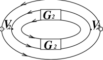
FIG. 4.: Pictorial demonstration of the Born approximation for $G_{6}(\Omega_{\mu})$. The dots indicate the Potential $V_{2}$. Exchange and rearrangement channels have to be added for a full treatment.

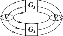
FIG. 5.: Approximation of $G_{6}$ with full treatment of the intermediate three-particle Green function.

REFERENCES

• [1] H. Stöcker and W. Greiner, Phys. Rep. 137, 277 (1986).
• [2] G. Bertsch and S. Das Gupta, Phys. Rep. 160, 189 (1988).
• [3] W. Cassing, W. Metag, U. Mosel, and K. Niita, Phys. Rep. 188, 363 (1990).
• [4] W. Bauer, C.-K. Gelbke, and S. Pratt, Ann. Rev. Part. Sci. 42, 77 (1992).
• [5] W. Bauer, Prog. Part. Nucl. Phys. 30, 45 (1993).
• [6] T. Alm, G.Röpke, W. Bauer, F. Daffin, and M. Schmidt, Nucl. Phys. A 587, 815 (1995).
• [7] S. Nagamiya, M.C. Lemaire, E. Moeller, S. Schnetzer, G. Shapiro, H. Steiner, and I. Tanihata, Phys. Rev. C 24, 971 (1981), and refs. therein.
• [8] G. Kunde, PhD. thesis, GSI Darmstadt (1994), unpublished.
• [9] D.O. Handzy et al., Phys. Rev. Lett. 75, 2916 (1995); F. Zhu, W.G. Lynch, D.R. Bowman, R.T. de Souza, C.K. Gelbke, Y.D. Kim, L. Phair, M.B. Tsang, C. Williams, and H.M. Xu, Phys. Rev. C 52, 784 (1995).
• [10] M. Baldo, U. Lombardo, and P. Schuck, Phys. Rev. C 52, 975 (1995).
• [11] M. Schmidt, G. Röpke, and H. Schulz, Ann. Phys. (NY) 202, 57 (1990).
• [12] T. Alm, G. Röpke, and M. Schmidt, Z. Phys. A 337, 355 (1990); G. Röpke, M. Schmidt, L. Münchow, and H. Schulz, Nucl. Phys. A 339, 587 (1983); T. Alm, L. Friman, G. Röpke, H. Schulz, ibid. A 551, 45 (1993); G. Röpke, Ann. Phys. (NY) 3, 145 (1994).
• [13] P. Danielewicz and G.F. Bertsch, Nucl. Phys. A 533, 712 (1991).
• [14] M. Beyer, G. Röpke, A. Sedrakian, Phys. Lett. B 376, 7 (1996).
• [15] G. Röpke, Phys. Rev. A 38, 3001 (1988).
• [16] D. Zubarev, V. Morozov, and G. Röpke, Statistical mechanics of nonequilibrium processes vol. I (Akademie Verlag, Berlin, 1996).
• [17] L.P. Kadanoff, G. Baym, Quantum Theory of Many-Particle Systems (Mc Graw-Hill, New York, 1962).
• [18] W.-D. Kraeft, D. Kremp, W. Eberling, G. Röpke, Quantum Statistics of Charged Particle Systems (Akademie-Verlag, Berlin, 1986).
• [19] J.I. Kapusta, Finite-temperature field theory in Cambridge Monographics on Mathematical Physics, eds. P.V. Landshoff, D.R. Nelson, D.W. Sciama, S. Weinberg (Cambridge University Press, Cambridge, 1989).
• [20] W. Glöckle, The Quantum Mechanical Few-Body Problem, (Berlin, New York, Springer, 1983); I.R. Afnan and A.W. Thomas in: Modern Three Hadron Physics ed. A.W. Thomas, p.1, (Berlin, Springer, 1977); E.W. Schmidt and H. Ziegelmann, The Quantum Mechanical Three-Body Problem, (Oxford, Pergamon Press, 1974); W. Sandhas, Acta Physica Austriaca, Suppl. IX, 57 (1972); V.B. Belyaev, Lectures on the Theory of Few-Body Systems (Spinger, Berlin 1990).
• [21] E.O. Alt, P. Grassberger, and W. Sandhas, Nucl. Phys. B 2, 167 (1967).
• [22] P. Schuck, Z. Phys. 241, 395 (1971); P. Schuck, F. Villars, P. Ring, Nucl. Phys. A 208, 302 (1973); J. Dukelsky, P. Schuck, Nucl. Phys. A 512, 466 (1990); P. Schuck, Nucl. Phys. A 567, 78 (1994).
• [23] W. Plessas et al., Few-Body Systems Suppl. 7, 251 (1994), and ref. therein.; L. Mathelitsch, W. Plessas, and W. Schweiger, Phys. Rev. C 26, 65 (1982); J. Haidenbauer and W. Plessas, Phys. Rev. C 30, 1822 (1984).
• [24] H. Witala, T. Cornelius, and W. Glöckle, Few-Body Systems 5, 89 (1988); J.L. Friar, G.L. Payne, W. Glöckle, D. Huber, and H. Witala, Phys. Rev C 51, 2356 (1995), and ref. therein.
• [25] T. Januschke, T.N. Frank, W. Sandhas, and H. Haberzettl, Phys. Rev. C 47, 1401 (1993); T.N. Frank, H. Haberzettl, T. Januschke, U. Kerwath, and W. Sandhas, Phys. Rev. C 83, 1112 (1988); Th. Januschke, PhD. Thesis, Bonn 1990, BONN-IR-90-52, unpublished.
• [26] V.G. Morosov and G. Röpke, Physica A 221, 511 (1995).
• [27] G. Röpke and H. Schulz, Nucl. Phys. A477, 472 (1988).
• [28] A.L. Fetter, J.D. Walecka, Quantum Theora of Many-Paricle Systems, (Mc Graw Hill, New York, 1971).
• [29] E.O. Fiset, Phys. Rev. C 2, 85 (1972).
• [30] W. Sandhas, Acta Physica Austriaca, Suppl. IX, 57 (1972).
• [31] G. Röpke and H. Schulz, Nucl. Phys. A 477, 472 (1988).
• [32] A.C. Phillips, Nucl. Phys. A 107, 209 (1968).
• [33] J. Brunisma and R. van Wageningen, Nucl. Phys. A 282, 1 (1977).
• [34] P. Schwarz et al., Nucl. Phys. A 398, 1 (1983).
• [35] G. Röpke, Statistische Mechanik für das Nichtgleichgewicht, (Deutscher Verlag der Wissenschaften, Berlin 1987).
Refer to caption