Abstract

We present a phenomenological model for the initial conditions needed in a one-fluid hydrodynamical description of ultrarelativistic nuclear collisions at CERN–SPS. The basic ingredient is the parametrization of the baryon stopping, i.e. the rapidity distribution, as a function of the thickness of the nuclei. We apply the model to S + S and Pb + Pb collisions and find after hydrodynamical evolution reasonable agreement with the data.

Talk given at the International Workshop on Applicability of Relativistic Hydrodynamical Models in Heavy Ion Physics, ECT*, Trento (Italy), May 12 – May 16, 1997

1 Introduction

One of the main motivations of heavy ion experiments is the investigation of the nuclear equation of state away from the ground state. However, it is very difficult to deduce from the final multi-particle state, i.e. from the experimental particle distributions, model independent statements about the equation of state. It is not even granted, that the time and volume available are large enough to create a form of matter which can be described using (infinite volume) thermodynamics. Nevertheless, the only possibility to obtain information on the equation of state at large temperatures and densities is via dynamical models of these collisions.

One popular approach to the dynamics of heavy ion collisions is the use of one-fluid hydrodynamics [1, 2, 3]. Hydrodynamical simulations at energies below 10 $A$ GeV (BEVALAC and SIS) usually start with the approaching nuclei before their initial impact and include the initial compression. In such a treatment the nuclei fuse to a single fluid, implying, at zero impact parameter, a complete stopping of equal size nuclei. At higher energies, as at the CERN–SPS, RHIC and LHC, this is not justified, and one must be able to incorporate nuclear transparency in the description. Instead of trying to describe the production and equilibration within hydrodynamics, one starts the calculation from initial conditions which specify the hydrodynamic state of the system at initial time $t_{0}$. Initial conditions parametrize the production and equilibration dynamics.

The aim of this article is to present a parametrization of the initial baryon stopping, i.e. initial baryon rapidity distribution, in terms of the thickness of the incoming nuclei. The parametrization should be valid for all symmetric collisions at a given cms energy. Here we concentrate on CERN–SPS collisions at $\sqrt{s}\approx 20$ GeV per nucleon. After having found such a parametrization there are only a few additional parameters left like, e.g. the initial time. This makes the determination of the initial state from experimental data, usually done by trial and error, less arbitrary.

2 Baryon Stopping

The experimental net baryon rapidity distribution $dN^{\rm B}/dy$ is in general a function of $\sqrt{s}$ and the mass numbers $A$ and $B$ of the colliding nuclei. The mass numbers determine the mean number of interactions which an individual nucleon suffers. The rapidity distribution of final free baryons, $dN^{\rm B}/dy\,(\sqrt{s},A,B)$, is measured in several experiments. However, since we want to study the evolution of the colliding system after its formation at time $t_{0}$, we need the knowledge of $dN^{\rm B}/dy$ at $t_{0}$. This information can only be obtained by models, which describe the initial production stage of the nuclear collision well. Cascade type models may in principle provide this information. Our approach is much simpler. All physics of baryon stopping is included in the parametrization of $dN^{\rm B}/dy$ with the final justification coming from the comparison to the experiment.

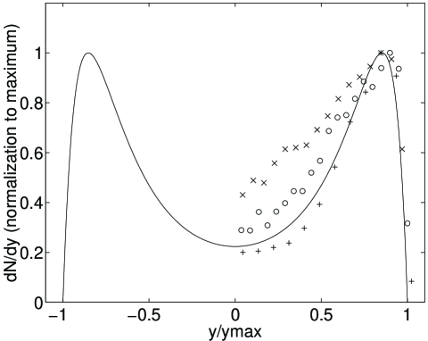
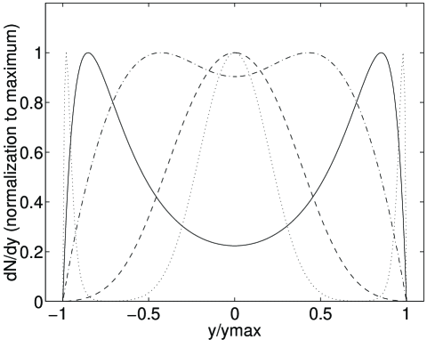
Figure 1: a) Rapidity distribution of protons in $p+p$ collisions for three different energies normalized to their maximum: Experimental data: ’x’ $\sqrt{s}=4.9$ GeV [4], ’o’ $\sqrt{s}=6.9$ GeV [4], ’+’ $\sqrt{s}=27.5$ GeV [5]; The line corresponds to the parametrization (2) described in the text.
b) Parametrization of the rapidity distribution of the initial baryons for various numbers of average nucleon–nucleon collisions $\langle n\rangle$ normalized to the maximum. Going from the edge to the center the lines correspond to $\langle n\rangle=0.1$ (dotted), $\langle n\rangle=1$ (full), $\langle n\rangle=2$ (dashed-dotted), $\langle n\rangle=4$ (dashed) and $\langle n\rangle=8$ (dotted). The line for $\langle n\rangle=1$ is the same as the parametrization in Fig. 1a.

To motivate our parametrization we start from what is known in $p+p$ collisions. In order to compare various collisions at different energies, we use the scaled rapidity $x_{y}=y/y_{max}$, where $y$ is measured in the cms frame of the colliding protons. In Fig. 1a we show the rapidity distribution $dN/dy$ of protons for three values of $\sqrt{s}$, plotted against $x_{y}$ and normalized to 1 at the maximum. Going from lower to higher energies, the central region ($y\approx 0$) becomes more depleted indicating increasing transparency of colliding nucleons with increasing $\sqrt{s}$. The maximum, however, seems to stay fixed around $x_{y}=0.85$ independent of $\sqrt{s}$.

In Fig. 1a we also show a parametrization of the $dN/dy$ as we interpolate the data to $\sqrt{s}=20$ GeV as appropriate for CERN–SPS nuclear collisions. The following consideration went into the parametrization. We compose the distribution out of two parts, one dominant in the target and the other in the projectile fragmentation region. The rise in $dN/dy$ going from the center to forward (or backward) regions is roughly exponential. Therefore we start out with two exponential functions of third order polynomials:

$$\frac{dN}{dy} = \frac{dN^{\rm Proj}}{dy}(x_{y})+\frac{dN^{\rm Tar}}{dy}(x_{y})=$$

$$\left[C_{\rm Proj}\exp(ax_{y}^{3}+bx_{y}^{2}+cx_{y})+C_{\rm Tar}\exp(-ax_{y}^{3}+bx_{y}^{2}-cx_{y})\right](1-x_{y}^{2})\>.$$

The factor $(1-x_{y}^{2})$ is chosen to cut off the distribution at the phase space boundary. The fit in Fig. 1a is given by $a=1.5$, $b=0$, $c=3.0$, and $C_{\rm Proj}=C_{\rm Tar}$ with values of $C$’s determined via the normalization.

We now assume that the initial baryon rapidity distribution $dN_{\rm B}/dy$ in a nuclear collision has the same functional form as Eq. (2), but the parameters $a,b$ and $c$ depend on the nuclear thickness a participating beam (target) nucleon sees on its way through the target (beam) nucleus. The task is to find this dependence.

The thickness function is defined as

$$T_{A}(\vec{\rho})=\int dz\;\rho_{A}(z,\vec{\rho})\>,$$ (2)

where $\rho_{A}(\vec{r})$ is the nuclear density for a nucleus of mass number $A$, $z$ is the longitudinal and $\vec{\rho}$ the transverse variable: $\vec{r}=(z,\vec{\rho})$. We take a Woods-Saxon parametrization for the nuclear density

$$\rho_{A}(\vec{r})=\frac{\rho_{0}}{\exp[(|\vec{r}|-R_{A})/a_{R}]+1}\>,$$ (3)

with

$$R_{A}=1.12\>{\rm fm}\times A^{1/3}-0.86\>{\rm fm}\times A^{-1/3}\,$$ (4)

$a_{R}=0.54$ fm, and $\rho_{0}=0.17$ fm^-3 [7].

We expect that the stopping depends not only on the thickness but also on an interaction strength, like the inelastic cross section. Then the natural quantity for the parametrization of stopping is

$$\langle n\rangle(\vec{\rho})=\sigma_{pp}\,T_{A}(\vec{\rho})\;,$$ (5)

where we use $\sigma_{pp}=32$ mb, the total inelastic cross section for $p+p$ collisions at SPS energy. In the Glauber model [6] $\langle n\rangle(\vec{\rho})$ is the average number of interactions suffered by a nucleon colliding with a nucleus at impact parameter $\vec{b}=\vec{\rho}$. The value of $\sigma_{pp}$ is not important since $\langle n\rangle$ will be multiplied by adjustable parameters. We should like to emphasize that $\langle n\rangle$ should be considered as a reasonable quantity to describe the strength of stopping of a nucleon and it need not be interpreted as the number of interactions except at the limit of small $\langle n\rangle$. In particular, for $\langle n\rangle=1$ we should have the same rapidity distribution as in $p+p$ collisions.

We impose the following limits. Since $|x_{y}|\leq 1$ the parameter $a$ becomes important at the edge of the phase space. For $T_{A}\rightarrow\infty$ we expect $a$ to vanish because the nucleons are shifted gradually to $x_{y}=0$. The limit $a\rightarrow 0$ is achieved by $a\propto 1/T_{A}$. More generally we could assume power behaviour but the inverse dependence turns out to be sufficient.

In Eq. (2) the actual stopping is expressed through the parameter $b$ which is zero for $\langle n\rangle=1$ and negative for $\langle n\rangle>1$, and should dominate for growing $\langle n\rangle$. We use a simple ansatz $b={\beta_{s}}\>(1-\langle n\rangle)={\beta_{s}}\>(1-\sigma_{pp}\,T_{A})$. The prefactor $\beta_{s}$ is a fit parameter characterizing the stopping. From fits to the experimental particle spectra we obtain $\beta_{s}=2.25$. One has to keep in mind that the deduced value of $\beta_{s}$ depends on the time evolution from initial to final distributions and therefore on the equation of state which is used. Finally, the parameter $c$ could also be chosen to depend on the thickness. However, it turns out that we can obtain the needed rapidity shift as a function of nuclear thickness from the $\langle n\rangle$ dependence of $b(\langle n\rangle)$ alone and leave $c$ as a constant.

We summarize the functional dependence of the parameters $a,b$ and $c$ on $T_{A}$:

$$a(T_{A}) = 1.5\>(\sigma_{pp}\,T_{A})^{-1}$$

$$b(T_{A}) = {\beta_{s}}\>(1-\sigma_{pp}\,T_{A})$$

$$c(T_{A}) = 3.0\>.$$ (6)

These functions (6) together with (2) form our phenomenological ansatz with the values of the parameters determined mainly from the S + S data. In Fig. 1b we show, with $\beta_{s}=2.25$ the resulting $dN_{\rm B}/dy$ for several values of $\langle n\rangle$ normalized as in Fig 1a. For $\langle n\rangle=1$ the curve is the same as in Fig. 1a. The dependence of $dN_{\rm B}/dy$ on $\langle n\rangle$ shows the following limits. For $\langle n\rangle\rightarrow 0$ the parameter $a(\langle n\rangle)$ dominates and leads to a sharp rise at $|x_{y}|\mathrel{\mathchoice{\lower 3.0pt\vbox{\halign{$\hfill#\hfil$\cr<\crcr\sim\crcr}}}{\lower 3.0pt\vbox{\halign{$\hfill#\hfil$\cr<\crcr\sim\crcr}}}{\lower 3.0pt\vbox{\halign{$\hfill#\hfil$\cr<\crcr\sim\crcr}}}{\lower 3.0pt\vbox{\halign{$\hfill#\hfil$\cr<\crcr\sim\crcr}}}}1$ which is cut down by the phase space factor at the boundaries. Therefore $dN_{\rm B}/dy$ turns to a double $\delta$-function peaked at target and projectile rapidity. For $\langle n\rangle\rightarrow\infty$, the parameter $b(\langle n\rangle)$ dominates and results in a Gaussian function for $dN_{\rm B}/dy$ which narrows with increasing $\langle n\rangle$.

Since we obtain the distribution as a function of transverse variable $dN_{\rm B}(\vec{\rho})/dy$ it will be normalized to the number of nucleons per unit transverse area at $\vec{\rho}$. To obtain the final local density we must know the dependence between rapidity and longitudinal distance $z$ at the initial time $t_{0}$. We do this by specifying the initial velocity profile by choosing a linear relation between rapidity and $z$:

$$y(\rho,z)=\kappa(\rho)z\,,\qquad v_{z}(\rho,z)=\tanh[\kappa(\rho)z]\>.$$ (7)

The local density $\rho_{B}(z,\rho)$ is obtained from the $dN_{\rm B}(\vec{\rho})/dy$ by multiplying with $(dy/dz)/\cosh y$ where $\cosh y$ is the Lorentz contraction factor between the local rest frame and the fixed cms frame. We will specify the initial flow velocity, in particular the $\vec{\rho}$ dependence of $\kappa(\rho)$, after discussing the initial energy distribution.

3 The Initial Energy Flow and Velocity Profile

The numerical solution of the hydrodynamical equations is determined on a 2 + 1 dimensional grid in the cylindrical coordinate system $\vec{r}=(z,\vec{\rho})$ [3]. The frame which we use is always the cms frame of the participating nucleons.

Since we assume azimuthal symmetry the simulation is strictly valid only for zero impact parameter collisions. However, even the triggering to 5% of most central events in the experiments corresponds to a considerable range in impact parameter. It turns out that if we incorporate the full energy available in the impact parameter zero collisions we slightly overshoot the experimental spectra. To account for the experimental impact parameter averaging, we use effective nuclear sizes, i.e. we replace the incoming nuclei $A,B$ by $A^{\rm eff}=\xi A$ and $B^{\rm eff}=\xi B$ and fix the geometry in terms of effective mass numbers $A^{\rm eff}$ and $B^{\rm eff}$. The value of $\xi$ is close to one. Our numerical algorithm for the calculation of final particle spectra leads to a few per cent loss of baryon number and energy [3]. We compensate also for these losses when fixing the value of $\xi$ to be 0.9 in symmetric collisions.

For the hydrodynamical calculation we need also the local energy density $\varepsilon(\vec{r})$ and the initial flow velocity at the initial time $t_{0}$. For the energy density we follow a similar approach as for the baryon density. We first parametrize the energy per unit transverse area and unit rapidity using a Gaussian distribution in rapidity

$$\frac{dE(\vec{\rho})}{dy}=C_{\varepsilon}\exp\left[\frac{-(y-y_{0})^{2}}{2\sigma_{\varepsilon}^{2}}\right]\>\left[1-(y/y_{max})^{2}\right]\>,$$ (8)

where the width $\sigma_{\varepsilon}$ and the normalization $C_{\varepsilon}$ depend on the transverse coordinate $\vec{\rho}$. The last factor is the same phase space cut-off as imposed for the baryons (2). Eq. (8) contains only the non-baryonic energy to which the contribution connected with the net baryon density will be added. The parametrization has three unknowns (at each $\vec{\rho}$), but only one, e.g. the width $\sigma_{\varepsilon}$ may be freely chosen. The normalization $C_{\varepsilon}$ is given by energy conservation, imposed per unit transverse area at each value of $\rho$. The value $y_{0}$ is the center of mass rapidity for nucleons at $\vec{\rho}$. For symmetric collision $y_{0}=0$ in the cms frame.

It turns out that the experimental pion rapidity distribution is well reproduced when the value of $\sigma_{\varepsilon}$ correlates with the baryon stopping. A larger stopping of baryon number results in a larger stopping of energy, too. Therefore the width of the energy distribution in rapidity space decreases with increasing nuclear stopping. We describe this with an ansatz

$$\sigma_{\varepsilon}(\rho)=\frac{c_{\varepsilon}}{\left[\sigma_{pp}T_{A}(\rho)\sigma_{pp}T_{B}(\rho)\right]^{\;\alpha_{\varepsilon}}}\>,$$ (9)

where $\sigma_{pp}$ is included in order to make the denominator dimensionless. The numbers appearing in (9) are determined from the fits to the symmetric collision systems: $c_{\varepsilon}=0.75$, $\alpha_{\varepsilon}=0.13$.

Next we add to the energy density Eq. (9) the energy density connected with the net baryon number. This additional energy is important at the edge of phase space and ensures that we take into account the rest mass and the thermal energy of every leading nucleon. We write the coordinate space density in the form

$$\varepsilon(\vec{\rho},z)=\frac{dE(\rho)}{dy}\>\frac{dy(\vec{\rho},z)}{dz}+\zeta\rho_{\rm B}(\vec{\rho},z)\>,$$ (10)

where $\zeta$ is the energy carried by the baryon. We take $\zeta=1.3\ {\rm GeV}\approx m_{\rm nuc}+E_{\rm th}$ where $m_{\rm nuc}$ is the rest mass of a nucleon and $E_{\rm th}$ its thermal energy. Since $\rho_{\rm B}$ is the net baryon distribution, the energy of baryon-antibaryon pairs is included in the first term.

The expansion of the matter is very sensitive on the initial velocity profile. Since we consider zero impact parameter collisions with cylindrical symmetry only, we do not expect significant collective motion in transverse direction initially, and take the velocity in the transverse direction at $t_{0}$ to vanish, i.e., $\vec{v}_{\rho}(t_{0},\vec{r})=0$.

In the case of the Bjorken model [10], the scaling ansatz for longitudinal velocity is $v_{z}=z/t$ and initial conditions are usually defined on fixed proper time $\tau_{0}$. At finite, albeit high collision energies, the longitudinal extent of the system is finite and the scaling assumption must break in the fragmentation regions. Since we perform the numerical calculations in the center-of-mass frame of the participating nucleons we specify the initial condition at a fixed time $t_{0}$ in this frame. On this line the scaling velocity is $z/t_{0}$. Since scaling cannot hold, we have, for convenience, chosen the linear $z$–dependence for rapidity instead of velocity as given in Eq. (7). For small $z$ this ansatz can approach the velocity profile of the scaling solution. The proportionality constant is now $\kappa$ instead of $1/t_{0}$ of the Bjorken model. We define $\tau_{0}^{\rm eff}=1/\kappa(\rho=0)$ as a parameter which can be regarded as an equilibration time scale in the same way as $\tau_{0}$ in the scaling case.

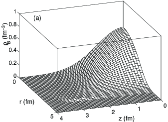
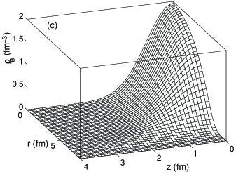
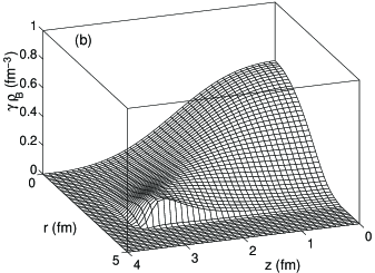
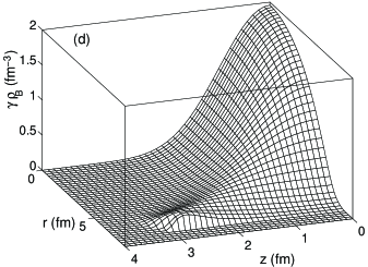
Figure 2: Local baryon density $\rho_{\rm B}$ (upper) and $\gamma\rho_{\rm B}$ (lower) in the $z$-$\rho$ plane as they result from the parametrization. The initial distribution is for S + S collisions (left) and Pb + Pb (right).

We determine the $\rho$ dependence of $\kappa(\rho)$ through the longitudinal extension of the system, $z_{L}(\rho)$, at different values of $\rho$. The $\rho$ dependence arises from the variation of the nuclear thickness in the transverse plane. The difference of the longitudinal extension between the center and the edge is of the order of $\Delta z=z_{L}(\rho=0)-z_{L}(\rho=R_{A})\approx R_{A}/\gamma$, where $\gamma=\cosh(y_{A})$ is the Lorentz contraction of the nucleus in the fireball rest frame. This form follows from nuclear geometry and the assumption that formation and equilibration times are independent of $\rho$. We define

$$z_{L}(\rho)=z_{0}+\frac{\sqrt{R_{A}^{2}-\rho^{2}}}{\gamma}\>,$$ (11)

where $z_{0}$ is the longitudinal extension of the matter at equilibration time in the thin disk limit. Instead of $z_{0}$ we use $\tau_{0}^{\rm eff}$ as an independent parameter with the assumption that the forward (backward) edge of the initial fireball, $z_{L}(\rho)$, moves with the target (projectile) rapidity $y_{\rm cms}$, which, from Eq. (7) at $\rho=0$ gives

$$z_{0}=\tau_{0}^{\rm eff}\;y_{\rm cms}-\frac{R_{A}}{\gamma}\>.$$ (12)

Combining the above definitions one gets

$$\kappa(\rho)=\frac{y_{\rm cms}}{z_{L}(\rho)}\>.$$ (13)

Even though the initial distributions approach zero in transverse direction as a consequence of the finite size of the nuclei (cf. Eq. (3)), it is still practical for the numerical work to make them zero beyond some value of $\rho$. As a criterium we use the mean value of interactions, $\langle n\rangle$ and set the initial distributions to zero when $\langle n\rangle<0.5$. It is clear that even so the matter at the edge is not dense enough for thermalization but for a finite system we are forced to extend the calculation at the surface to densities were the hydrodynamics cannot be justified.

We show in Fig. 2 the resulting initial baryon density distributions for S + S and Pb + Pb. The upper frames give the densities in the local comoving frame and the lower the spatial density in the overall rest frame of the collision. The difference comes from the $\gamma$ factor of the Lorentz contracted fluid cell. The figure clearly shows the increase in transparency with radius. We think this is more reasonable than using the same baryon distribution at the edge as at the center. In this figure the cut in $\langle n\rangle$ leads to a sharp discontinuity in radial directions near the maximum. However, this does not influence the dynamics, because the pressure gradients are given by the local densities, which are small and smooth in this region when going to larger $\rho$ as seen in the two upper figures.

In Tab. 1 we give the values of parameters which characterize the initial state. An interesting point is that $\tau^{\rm eff}_{0}$ which is a parameter adjusted to each collision system turns out to be rather similar in Pb + Pb and S + S collisions. This means that the equilibration time seems to be independent of the thickness of the nuclei.

Table 1: Summary of parameters characterizing the collision when a QGP equation of state is used. $\xi$ and $\tau^{\rm eff}_{0}$ are parameters adjusted to the data and explained in the text. The rest follows from the initial parametrization. $t_{f}$ is the central freeze-out time and $\langle v_{\rho}\rangle$ the mean radial velocity in the rapidity range of $|y_{z}|<0.25$.

collision	S + S	Pb + Pb
$\xi$	0.9	0.9
$\tau^{\rm eff}_{0}$ (fm/c)	1.2	1.3
$z_{L}(0)$ (fm)	3.5	3.6
cent. $\varepsilon$ (GeV/fm3)	7.1	16.7
cent. $\rho_{\rm B}$ (fm-3)	0.59	1.94
cent. $T$ (MeV)	244	300
$R(\xi A)$ (fm)	3.15	6.25
$t_{f}$ (fm/c)	6.1	11.4
$\langle v_{\rho}\rangle(|y_{z}|<0.25)$	0.28	0.34

4 Results

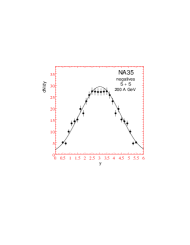
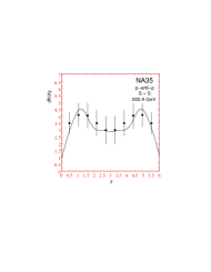
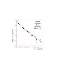
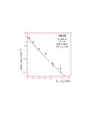
Figure 3: Comparison of experimental data from S + S collisions with final hadron spectra calculated using an equation of state (EOS A) with phase transition at $T_{c}=165$ MeV. The data are taken by the NA35 collaboration [11].

We illustrate the use of the parametrization of initial conditions discussed above by comparing with experimental data from the NA35 [11] and NA49 [9] collaborations. We solve the hydrodynamical evolution as described in [3], where also the treatment of the freeze-out is explained. We use isospin symmetry when calculating the hadron spectra. The isospin corrections would somewhat reduce the calculated $p-\bar{p}$ spectrum in the heavy systems (e.g. Pb + Pb) but our choice $\xi=0.9$ probably overestimates the amount of spectator nucleons. The freeze-out happens at a constant energy density of $\varepsilon_{f}=0.15\;{\rm GeV/fm}^{3}$ leading to an average freeze-out temperature of $T_{f}\approx 140$ MeV. In [3] we also explain the construction of the equation of state we use. Here we show results only for an equation of state with phase transition to QGP at $T_{c}=165$ MeV, labeled as EOS A in [3].

The stopping shows up mainly in the rapidity distributions. We show in Fig. 3 the distributions for negatives and proton-antiproton difference in a central S + S collision. In the $p-\bar{p}$ rapidity distribution target and projectile fragmentation regions exhibit clear maxima, which are nicely reproduced by the calculation. The normalization is slightly adjusted by the $\xi$ parameter. The rapidity distribution of the negatives fits very well. Also the transverse momentum distributions of both negatives and $p-\bar{p}$ are reproduced reasonably well.

Fig. 4 shows the result for Pb + Pb collisions compared with preliminary data from the NA49 collaboration [9]. There are small deviations in the proton distribution but the negative particle rapidity distribution is very well reproduced. Both collisions are calculated with nearly the same parametrization, the difference coming from the thickness function $T_{A}(\rho)$ only. The only slight difference is the $\tau_{0}^{\rm eff}=1.2$ for S + S and $\tau_{0}^{\rm eff}=1.3$ for Pb + Pb. Thus the parametrization reproduces well the stopping as a function of nuclear size. The result for $p-\bar{p}$ show larger deviation with faster protons in the experimental spectrum than in the calculated result. At least part of this must come from the finite impact parameter range included in the measurement and leading to a larger average transparency. In the calculation we take this into account only in the normalization through the parameter $\xi$ with practically no change in the shape of the spectrum.

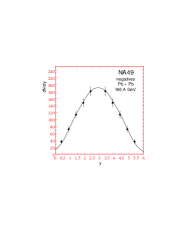
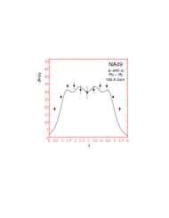
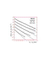
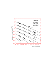
Figure 4: Comparison of experimental data from Pb = Pb collisions with final hadron spectra calculated using an equation of state (EOS A) with phase transition at $T_{c}=165$ MeV. The data are taken by the NA49 collaboration [9] and should be considered as preliminary. The $m_{T}$-spectra of negatives and $p-\bar{p}$ are measured in rapidity intervals of width 0.5 centered at 2.9 ($p-\bar{p}$ only), 3.4, 3.9, 4.4, 4.9, 5.4. For clarity the data and the calculation are successively scaled down by $10^{-n}$ ($n=0$,1,2,…).

The gross features of the transverse momentum data of the negative particles are again well reproduced except for the very forward (and backward) region were the calculated slope is steeper than the data. The particle density at this edge of the phase space, however, is becoming so small that the hydrodynamics with relatively strong longitudinal flow can lead to an artificially large transverse cooling. Thus we should not expect that hydrodynamics can describe the far edges of fragmentation regions well.

This problem is more pronounced in the $p-\bar{p}$ transverse distributions which indicate that even in the central rapidity region the experimental transverse flow is somewhat stronger. A possible explanations is that the equation of state is too soft. Later freeze-out time might also enhance the flow effect on protons as compared to pions.

In Tab. 1 we also give numbers which characterize the freeze-out. The lifetime $t_{f}$ of the fireball, measured at the center, scales as expected with the size of the fireball. We see a doubling of the lifetime going from S + S to Pb + Pb in accordance with the doubled radius of the lead nucleus. We further give the average (radial) transverse velocity $\langle v_{\rho}\rangle$ of the fluid cells at freeze-out with rapidity $|y_{z}|<0.25$. The result may be compared with an analysis of NA44 [12]. They extracted from a fit to hadron data a mean transverse velocity. The result is [12] $\langle v_{\rho}\rangle=0.24\pm 0.10$ for S + S and $\langle v_{\rho}\rangle=0.36\pm 0.14$ for Pb + Pb in agreement with our studies. However, the NA44 obtained a higher freeze-out temperature for Pb + Pb, $T_{f}=167\pm 13$ MeV (for S + S $T_{f}=142\pm 5$ MeV). This explains why NA44 gets agreement with $\langle v_{\rho}\rangle=0.36$ while we slightly underestimate the slope in the central $p-\bar{p}$ transverse momentum spectra.

Finally we compare our results with the related work of Schlei et al. [2]. (See also [13] in this Volume, where a different parameter set for initial conditions is used.) The main difference is in the geometry of the initial fireball. The equations of state differ slightly. Both exhibit a phase transition to QGP, ours with $T_{c}=165$ MeV vs. 200 MeV in [2]. In addition, the baryonic pressure in [2] is omitted.

The basic differences may be summarized in the following way. The calculation in [2] starts from a small longitudinal extension, indicating large compression, and resulting in larger initial energy density as compared to ours. At the center of the fireball for S+S collision $\epsilon_{i}=13.0$ GeV/fm³ in [2] vs. 7.1 GeV/fm³ in our case. For Pb+Pb the numbers are 20.4 GeV/fm³ and 16.7 GeV/fm³, respectively. At first glance this looks like a difference in stopping but a closer inspection shows that it is related more closely to the initial volume than to the initial velocity distribution. This can be interpreted as a difference in initial time, our calculation corresponding to a later initial time. If the energy stopping is characterized with the fraction of thermal energy, the numbers are very similar: 0.43 (0.64) in [2] vs. our 0.45 (0.66) for S+S (Pb+Pb). The difference in initial volume is related to the longitudinal extent and our larger initial volume can be interpreted as starting the calculation at later initial time. This shows up also as shorter lifetimes in our calculation, 6.1 fm/c vs. 6.9 fm/c in [2] for S+S and 11.4fm/c vs. 13.5 fm/c in [2] for Pb+Pb collisions.

5 Conclusions

A model for initial conditions was developed with a parametrization of baryon stopping in terms of the nuclear thickness as the basic input. The same parametrization gives a very satisfactory description of the basic features of hadron spectra both in S + S and Pb + Pb collisions. We think that this is an improvement compared to earlier approaches [2, 3] where the transverse dependence of stopping was not taken into account.

ACKNOWLEDGMENT
This work was supported by the Bundesministerium für Bildung und Forschung (BMBF) grand no. 06 BI 556 (6) and the Academy of Finland grant no. 27574.

References

-
[1]
For reviews see:
H. Stöcker and W. Greiner, Phys. Rep. 137, 277 (1986); R.B. Clare and D. Strottman, Phys. Rep. 141, 177 (1986); J.P. Blaizot and J.Y. Ollitraut, Quark-Gluon Plasma, edited by R.C. Hwa (World Scientific, Singapore, 1990). - [2] B.R. Schlei, U. Ornik, M. Plümer, D. Strottman, and R.M. Weiner Phys. Lett. 376B, 212 (1996); U. Ornik, M. Plümer, B.R. Schlei, D. Strottman, and R.M. Weiner, Los Alamos preprint LA-UR-96-1615, August 1996, nucl-th/9608027
- [3] J. Sollfrank, P. Huovinen, M. Kataja, P.V. Ruuskanen, M. Prakash, and R. Venugopalan, Phys. Rev. C 55, 392 (1997).
- [4] V. Blobel et al., Nucl. Phys. B69, 454 (1974).
- [5] M. Aguilar–Benitez et al. (NA27 collaboration), Z. Phys. C 50, 405 (1991).
- [6] R.J. Glauber, in Lectures in Theoretical Physics, edited by W.E. Brittin and L.G. Dunham (Interscience, New York, 1959), Vol. 1, p. 315
- [7] A. Bohr and B.R. Mottelson, Nuclear Structure, Vol. 1, (W.A. Benjamin,Inc, New York, 1969)
- [8] J. Sollfrank, P. Huovinen, and P.V. Ruuskanen, in preparation.
- [9] P.G. Jones et al. (NA49 collaboration), Nucl. Phys. A610, 188c (1996).
- [10] J.D. Bjørken, Phys. Rev. D 27, 140 (1983).
- [11] J. Bächler et al. (NA35 collaboration), Phys. Rev. Lett. 72, 1419 (1994)
- [12] I.G. Bearden et al. (NA44 collaboration), Phys. Rev. Lett. 78, 2080 (1997).
- [13] B. Schlei, this Volume.