Preprint Numbers: KSUCNR-101-97 nucl-th/9705018

We review recent progress in modeling the quark-gluon content of mesons and their low-energy interactions through the Global Color Model field theory. An emphasis is placed on techniques that are shared with the approach based on truncations of the Dyson-Schwinger equations of QCD. In contrast to most other field theory models for QCD degrees of freedom in hadron physics, this approach directly deals with the derived intrinsic space-time extent of the meson modes in their role as field variables and can accommodate confinement as well as dynamical breaking of chiral symmetry. Various theoretical techniques and approximations found useful in this approach are described. Selected applications reviewed here include the properties and interactions of the Goldstone bosons, interaction vertex functions, low energy chiral observables, electromagnetic interactions and form factors, and transition form factors. Some initial considerations of Vector Meson Dominance and pion loop processes are discussed.

KEYWORDS

hadrons from quarks and gluons; non-perturbative QCD modeling; confinement; dynamical chiral symmetry breaking; composite, finite size mesons; meson interaction and transition form factors; electromagnetic coupling; vector meson and pion loop processes.

1 Introduction

To investigate hadron physics from the perspective of nonperturbative quantum chromodynamics (QCD) and QCD-based models, a number of approaches are currently employed. These include the intensive computational method of lattice gauge field theory, the method of light cone quantization, QCD sum rules and chiral perturbation theory (ChPT). In one sense, the first two constitute a completely fresh start in that much of the empirical information on hadron dynamics that has been built up over many of the past decades through the refinement of model hadronic lagrangians is not easily joined. This becomes irrelevant when S-matrix elements for many-body hadronic processes can be routinely obtained from the relativistic gauge field theory of quarks and gluons. However it is apparent that for some time to come, model hadronic theories remain an important intermediate form into which new findings about non-perturbative QCD can be packaged for rapid deployment in hadron physics. One way to link QCD with such an intermediate form is to subject the quark-gluon action to a restructuring or change of field variables to expose hadronic or collective degrees of freedom and integrate out the quarks and gluons. At present, most work of this type that is able to confront a variety of hadronic observables deals with QCD-based model field theories. We review meson physics obtained from the Global Color Model (GCM) of QCD (Cahill and Roberts, 1985; Praschifka et al., 1987a). Other overviews of this model that emphasize different aspects can be found in Cahill (1992) and in Cahill and Gunner (1997).

What we refer to as a model hadronic field theory was in the past usually called an effective field theory. In either case this is in the old-fashioned sense that implies a semi-phenomenological model field theory meant for a limited low energy domain; but not implying an equivalent representation of an underlying theory through a systematic expansion and a counting scheme to order corrections. To distinguish the former from ChPT and other recent developments in hadron physics that are referred to as effective field theories in the technical sense, we shall use the terms model or approximate field theories.

The GCM is a model field theory of quarks in which the interaction is between quark color currents mediated by an effective $2$-point gluon function. The infrared form of the latter is the phenomenological element of the model, while it is constrained to match the known perturbative QCD behavior in the ultraviolet. The point coupling limit gives the closely related and widely used Nambu–Jona-Lasinio (NJL) model (Nambu and Jona-Lasinio, 1961) that is simpler to work with. Special interest is taken here in the distinguishing features of the GCM that include a naturally accommodated confinement mechanism and the finite size of the $\bar{q}q$ meson modes. The derived interactions between these modes produce vertex form factors that are accountable to underlying quark-gluon dynamics. It is this aspect that may provide an interesting perspective to the thrust in nuclear theory that centers around hadronic field theory models. A key question is whether a consistent quark-gluon basis can be developed for important hadron interaction vertices that can support the present empirical description (especially of the form factors) thus correlating many hadronic parameters with far fewer sub-hadronic parameters.

The Dyson-Schwinger equation (DSE) approach to non-perturbative QCD (Roberts and Williams, 1994) is to truncate the infinite system of coupled equations that link the $n$-point functions of QCD at low order, use an Ansatz to replace the discarded information, and to seek a self-consistent solution. There is a close correspondance in form between the content of the GCM action at tree-level in the composite hadron fields and a particular low-order implementation of the DSE approach. For this reason, a number of present calculations in each approach share common elements. A clearer distinction would become evident at the next level of treatment where the organization of the physics in each approach is different. However, they remain complementary; each providing insights into the role of nonperturbative QCD effects in hadron physics. We shall refer extensively to the mixing of elements of these approaches.

In Sec. 2 we introduce the Global Color Model and review the auxiliary field method for bosonization to an action for the meson modes of the theory. Also considered there is the decomposition to local field variables and the identification of the corresponding meson-quark vertex functions. That section ends with a discussion of issues related to extraction of physics from the formalism and calculations defined in Euclidean metric, and the relationship of the GCM and DSE approaches. Important elements for producing hadron observables from the GCM are the dressed quark propagators and forms used to facilitate calculations are summarized in Sec. 3. We examine in Sec. 4 the GCM description of the Goldstone boson sector, selected low energy chiral observables and methods used for other mesons. Electromagnetic coupling is developed in Sec. 5 where recent calculations of the pion and kaon charge form factors are reviewed. Meson interaction and transition form factors are discussed in Sec. 6. In Sec. 7 selected issues beyond meson tree level are considered and these include vector meson dominance processes and pion loop contributions. Concluding remarks are presented in Sec. 8.

2 Global Color Model

The action for the GCM is defined in Euclidean metric as (Cahill and Roberts, 1985; Praschifka et al., 1987a)

$$S_{GCM}[\bar{q},q]=\int d^{4}x\;\bar{q}(x)\bigl{(}\gamma\cdot\partial_{x}+m\bigr{)}q(x)+\mbox{\small$\displaystyle\frac{1}{2}$}\int d^{4}xd^{4}y\;j_{\mu}^{a}(x)\,g^{2}D_{\mu\nu}(x-y)\,j_{\nu}^{a}(y),$$ (2.1)

where $m$ is a diagonal matrix of bare quark masses, and $j_{\nu}^{a}(x)=\bar{q}(x)\frac{\lambda^{a}}{2}\gamma_{\nu}q(x)$ is the quark colored current. The employed Euclidean metric is such that $a\cdot b=a_{\mu}b_{\mu}$, spacelike vectors satisfy $a^{2}>0$, and $\{\gamma_{\mu},\gamma_{\nu}\}=$$2\delta_{\mu\nu}$, with $\gamma_{\mu}=\gamma_{\mu}^{\dagger}$. A model field theory of this form can summarize a number of diverse investigations in the modeling of hadron physics such as Cahill and Roberts (1985), McKay and Munczek (1985), Barducci et al. (1988), and McKay et al. (1989). This model may be viewed as a truncation of QCD and some consideration of that aspect can indicate the content and role that should be attributed to the phenomenological gluon two point function $D_{\mu\nu}$. The connections between QCD and Eq. (2.1) have been considered by Cahill and Roberts (1985) and by McKay et al. (1989) and a brief summary follows. Functional integral methods are convenient for that purpose. In QCD (see, e.g. Marciano and Pagels, 1978) the generating functional for quark propagators is

$$Z[\bar{\eta},\eta]=N\int D\bar{q}DqDA\>{\rm exp}\left(-S[\bar{q},q,A]+\int d^{4}x\;(\bar{\eta}q+\bar{q}\eta)\right),$$ (2.2)

where

$$S[\bar{q},q,A]=\int d^{4}x\left(\bar{q}(\mbox{$\not\!\partial$}+m-ig\frac{\lambda^{a}}{2}\mbox{$\not\!\!A$}^{a})q+\mbox{\small$\displaystyle\frac{1}{4}$}F^{a}_{\mu\nu}F^{a}_{\mu\nu}\right),$$ (2.3)

and $F^{a}_{\mu\nu}=\partial_{\mu}A^{a}_{\nu}-\partial_{\nu}A^{a}_{\mu}+gf^{abc}A^{b}_{\mu}A^{c}_{\nu}$. We leave the gauge fixing term, the ghost field term and its integration measure to be understood. If we introduce

$${\rm exp}\left(W[J]\right)=\int DA\>{\rm exp}\left(-\int d^{4}x\>(\mbox{\small$\displaystyle\frac{1}{4}$}F^{a}_{\mu\nu}F^{a}_{\mu\nu}-J^{a}_{\mu}A^{a}_{\mu})\right),$$ (2.4)

the generating functional becomes

$$Z[\bar{\eta},\eta]=N\int D\bar{q}Dq\>{\rm exp}\left(-\bar{q}(\mbox{$\not\!\partial$}+m)q+\bar{\eta}q+\bar{q}\eta\right)\;{\rm exp}\left(W\left[ig\bar{q}\frac{\lambda^{a}}{2}\gamma_{\mu}q\right]\right)~{},$$ (2.5)

where the abbreviated notation implies the usual spacetime integration. The functional $W[J]$ is the generator of connected gluon $n$-point functions without quark-loop contributions. It may be written as

$$W[J]=\mbox{\small$\displaystyle\frac{1}{2}$}\int d^{4}xd^{4}y\>J^{a}_{\mu}(x)D_{\mu\nu}(x-y)J^{a}_{\nu}(y)+W_{R}[J]$$ (2.6)

allowing the formal factorization

$$Z[\bar{\eta},\eta]={\rm exp}\left(W_{R}\left[ig\frac{\delta}{\delta\eta}\frac{\lambda^{a}}{2}\gamma_{\mu}\frac{\delta}{\delta\bar{\eta}}\right]\right)Z_{GCM}[\bar{\eta},\eta].$$ (2.7)

Here the quark field variables in the argument of $W_{R}$ have been replaced by the corresponding source derivatives. The truncated model identified this way is generated from

$$Z_{GCM}[\bar{\eta},\eta]=N\int D\bar{q}Dq\>{\rm exp}(-S_{GCM}[\bar{q},q]+\bar{\eta}q+\bar{q}\eta),$$ (2.8)

where $S_{GCM}[\bar{q}q]$, is given by Eq. (2.1) in which the dependence upon the coupling constant $g$ has been made explicit. The GCM corresponds to the retention of just the first term of Eq. (2.6), involving the gluon $2$-point function excluding $\bar{q}q$ vacuum polarization contributions. The neglected term $W_{R}$ involves the $n$-point functions, $n\geq 3$, from the pure gauge sector. Whether this can successfully model soft hadron physics can only be judged by consideration of the results that follow from a consistent phenomenological form for $g^{2}D_{\mu\nu}(x-y)$. Certainly, any element of hadron physics that absolutely requires the gluonic coupling of three or more quark currents can be expected to resist description via the GCM; that finding in itself would constitute a valuable contribution. On the other hand, if a significant body of information can be correlated through a phenomenological gluon $2$-point function via accessible continuum calculations, this might highlight those aspects that deserve more concentrated attention through lattice-QCD methods (Rothe, 1992). Even though the model in Eq. (2.1) looks Abelian in form (QED may be recast that way), the non-Abelian nature of the gauge field sector has not been totally ignored. Those non-Abelian aspects that contribute to the dressed pure-glue $2$-point function can be implemented through the phenomenological element of the GCM.

2.1 Bosonization to Mesons

The auxiliary field method consists of a transformation of a field theory that introduces additional field variables through which important dynamical features can be revealed more readily than with the original fields. The method has found wide use in statistical mechanics as the Hubbard-Stratonovich transformation (Stratonovich, 1957; Hubbard, 1959). Early applications of the auxiliary field method to quark dynamics (Eguchi and Sugawara, 1974; Kikkawa, 1976; Kleinert, 1976a) were applied to four-fermion interaction models of the NJL type. Here the auxiliary fields are introduced so as to assume the role of hadronic collective modes generated by combinations of $\bar{q}(x)$ and $q(x)$ at the same space-time point. The four-fermion interaction is exactly transformed into boson mass terms plus a local Yukawa coupling of boson fields to the quarks. The locality of the auxiliary boson fields is a consequence of the contact nature of the original four-fermion interaction. Since there remains only a quadratic dependence upon the quark fields, they could then be integrated out leaving a bosonized action. Expansion of the action in quantum fluctuations about the classical values of these composite fields was used to produce an effective action from which a number of important issues, e.g. renormalizability of four-fermion coupling (Eguchi, 1976) could be addressed.

It was subsequently observed (Kleinert, 1976b; Shrauner, 1977) that the auxiliary field method can be generalized to account for the intrinsic nonlocality in the quark couplings generated by models that have an Abelian vector gauge field coupled to quarks. The vector gauge field can be integrated out to produce a finite range four-fermion interaction. The auxiliary boson fields needed to reduce this interaction to quadratic form are bilocal combinations of $\bar{q}(x)$ and $q(y)$ whose free-field solutions turn out to be the ladder Bethe-Salpeter (BS) bound states. Expansion of the bilocal field in terms of these BS free-field eigenmodes produces (Kleinert, 1976b; Kugo, 1978) an effective action for the finite-size $\bar{q}q$ mesons of the model.

In these works color was omitted and baryons were not considered. The achieved reformulations in terms of $\bar{q}q$ objects constitute a true hadronization for the case of a single Abelian vector gauge field coupled to any number of flavors of quarks. Such a field theory shares many properties in common with the strong interaction such as the conserved vector currents, global $SU(N_{f})\otimes SU(N_{f})$ chiral symmetry, and the consequent PCAC. Nevertheless, to obtain insight into approximate methods for QCD in the nonperturbative domain of hadron physics, a study was begun (Cahill and Roberts, 1985) on the bilocal field hadronization method for colored quarks that interact through finite range coupling of their colored vector currents.

We shall consider only the Feynman-like gauge where $g^{2}D_{\mu\nu}(x-y)=\delta_{\mu\nu}D(x-y)$ and an Ansatz for $D$ defines the model. This is done to permit the simplest form of the reordering identities that are to follow. It should not be taken to imply that the intent is to match with information from a corresponding gauge choice in QCD. Such a choice is not possible as the above Ansatz will depart from the perturbative form in both transverse and longitudinal parts while the latter will have no interaction or dressing in QCD. A reformulation of $S_{GCM}$ in terms of fields that represent $\bar{q}q$ objects is achieved by the Fierz reordering identities

$$\gamma^{\mu}_{ij}\gamma^{\mu}_{kl}=K^{a}_{il}K^{a}_{kj}\;,\;\;\;K^{a}=({\bf 1},i\gamma_{5},\mbox{\small$\displaystyle\frac{i}{\sqrt{2}}$}\gamma_{\nu},\mbox{\small$\displaystyle\frac{i}{\sqrt{2}}$}\gamma_{\nu}\gamma_{5})$$ (2.9)

for spin,

$$\delta_{ij}\delta_{kl}=F^{b}_{il}F^{b}_{kj}\;,\;\;\;F^{b}_{N_{f}=2}=(\mbox{\small$\displaystyle\frac{{\bf 1}}{\sqrt{2}}$},\mbox{\small$\displaystyle\frac{\vec{\tau}}{\sqrt{2}}$})\;,\;\;\;F^{b}_{N_{f}=3}=(\mbox{\small$\displaystyle\frac{{\bf 1}}{\sqrt{3}}$},\mbox{\small$\displaystyle\frac{\lambda^{a}}{\sqrt{2}}$})$$ (2.10)

for flavor $SU(2)$ singlet plus triplet (${\bf 1}_{f}+{\bf 3}_{f}$), or $SU(3)$ singlet plus octet (${\bf 1}_{f}+{\bf 8}_{f}$), and

$$\lambda^{a}_{ij}\lambda^{a}_{kl}=C^{c}_{il}C^{c}_{kj}\;,\;\;\;C^{c}=(\mbox{\small$\displaystyle\frac{4}{3}$}{\bf 1},\mbox{\small$\displaystyle\frac{i}{\sqrt{3}}$}\lambda^{a})$$ (2.11)

for color $SU(3)$ singlet plus octet (${\bf 1}_{c}+{\bf 8}_{c}$). With the direct product set of matrices $\Lambda^{\theta}=\frac{1}{2}K^{a}\otimes F^{b}\otimes C^{c}$ where $\theta=(a,b,c)$, the complete reordering needed to express the the quartic quark current-current coupling in terms of a quadratic coupling of $\bar{q}q$ objects is

$$\left(\mbox{\small$\displaystyle\frac{\lambda^{a}}{2}$}\gamma_{\mu}{\bf 1}_{F}\right)_{ij}\left(\mbox{\small$\displaystyle\frac{\lambda^{a}}{2}$}\gamma_{\mu}{\bf 1}_{F}\right)_{kl}=\Lambda^{\theta}_{il}\;\Lambda^{\theta}_{kj},$$ (2.12)

and we use the summation convention for repeated indices. Hence in Eq. (2.1), this reordering causes $q(x)$ to form a scalar product with $\bar{q}(y)$ and $\bar{q}(x)$ with $q(y)$. An equivalent form that is useful later is

$$\mbox{\small$\displaystyle\frac{\lambda^{a}}{2}$}\gamma_{\mu}{\bf 1}_{F}\>M\>\mbox{\small$\displaystyle\frac{\lambda^{a}}{2}$}\gamma_{\mu}{\bf 1}_{F}=\Lambda^{\theta}\>{\rm tr}\>(\Lambda^{\theta}M)$$ (2.13)

where $M$ is any matrix. The Dirac matrix $\sigma_{\mu\nu}$ does not appear in Eq. (2.9) due to the use of the Feynman-like gauge. If one chooses a family of gauges parameterized by $\xi$, a more complicated Fierz reordering involving $\sigma_{\mu\nu}$ and $\xi$-dependent weights of the spin matrices is obtained. Because of the phenomenological nature of the effective gluon propagator here, the simplifications of the Feynman-like gauge are appealing.

With Eq. (2.12) the GCM action in Eq. (2.1) can be written as

$$S[\bar{q},q]=\int d^{4}x\>\bar{q}(x)\bigl{(}\gamma\cdot\partial_{x}+m\bigr{)}q(x)-\mbox{\small$\displaystyle\frac{1}{2}$}\int d^{4}xd^{4}y\>{\cal J}^{\theta}(x,y)^{*}D(x-y){\cal J}^{\theta}(x,y),$$ (2.14)

where the negative sign arises from the anticommuting property of the Grassmann variables $q$ and $\bar{q}$. There appear now bilocal currents ${\cal J}^{\theta}(x,y)=$ $\bar{q}(x)\Lambda^{\theta}q(y)$ that are hermitian, i.e. $[{\cal J}^{\theta}(x,y)]^{*}=$ ${\cal J}^{\theta}(y,x)$, and carry the Lorentz and flavor indices of the candidate $\bar{q}q$ states of this model. However the color structure of the $\bar{q}q$ combinations consists of the singlet ${\bf 1}_{c}$ as well as the octet ${\bf 8}_{c}$. The latter may be eliminated in favor of diquark correlations as discussed later.

As a specific illustration of the content of the interaction in Eq. (2.14), consider, for $N_{f}=2$, the point coupling limit where $D(x-y)\rightarrow\tilde{G}\delta(x-y)$. The $\Lambda^{\theta}$ in the color singlet channel are

$$\Lambda^{\theta}=\mbox{\small$\displaystyle\frac{\sqrt{2}}{3}$}\tau^{\alpha}\left\{{\bf 1}_{D},i\gamma_{5},\mbox{\small$\displaystyle\frac{i}{\sqrt{2}}$}\gamma_{\nu},\mbox{\small$\displaystyle\frac{i}{\sqrt{2}}$}\gamma_{\nu}\gamma_{5}\right\},$$ (2.15)

where $\alpha=0,1,2,3$ and $\tau^{0}=1$. It is convenient to separate out numerical factors $n_{\theta}$ and deal with the canonical set of matrices $\kappa_{\theta}$ defined by

$$\kappa_{\theta}=\frac{\Lambda^{\theta}}{n_{\theta}}=\tau^{\alpha}\left\{{\bf 1}_{D},i\gamma_{5},i\gamma_{\nu},i\gamma_{\nu}\gamma_{5}\right\}.$$ (2.16)

Then the interaction term from Eq. (2.14) in the color singlet sector becomes

$$S_{int}^{NJL}=-\mbox{\small$\displaystyle\frac{1}{2}$}\int d^{4}x\>\left\{G_{S}\left[(\bar{q}\tau^{\alpha}q)^{2}+(\bar{q}i\gamma_{5}\tau^{\alpha}q)^{2}\right]+G_{V}\left[(\bar{q}i\gamma_{\nu}\tau^{\alpha}q)^{2}+(\bar{q}i\gamma_{\nu}\gamma_{5}\tau^{\alpha}q)^{2}\right]\right\}.$$ (2.17)

Here $G_{S}=\frac{2}{9}\tilde{G}$, and $G_{V}=\frac{1}{9}\tilde{G}$. This is one of the simplest forms of the Nambu–Jona-Lasinio model (NJL) (Nambu and Jona-Lasinio, 1961) as applied to quarks in the color singlet channel. For recent reviews of the NJL model as applied to hadron physics, see Vogl and Weise (1991) and Klevansky (1992). The coupling constant relation $G_{S}=2G_{V}$ evident here has its origin in the simple coupling of quark color currents. Applications are usually made from the point of view of an effective model that implements chiral symmetry and its dynamical breaking; the constants $G_{S}$ and $G_{V}$ are allowed to be independent and are fitted to data. The GCM retains the distributed coupling of the $\bar{q}q$ correlations via an effective gluon $2$-point function $D(x-y)$ and also maintains the relative Fierz weighting that accompanies that function to each meson channel. For large momentum $q^{2}$, the magnitude of $D(q^{2})$ in the GCM is fixed by the requirement that perturbative QCD should be obeyed; this is not possible in the NJL since the constants $G_{S}$ and $G_{V}$ force the same coupling strength in the UV as in the IR. The role asked of phenomenology is quite different in the two models and the outcome can also be quite different.

We return now to Eq. (2.14) and before restructuring it, we note that the interaction term in Eq. (2.14) is explicitly chirally symmetric as is its original form. However that is not true for a fixed value of the summation index $\theta$. If one is to truncate that sum, it is necessary to retain a subset terms that mix under the chiral transformation to preserve the symmetry. Similarly for any symmetry e.g. an electromagnetic gauge transformation. The four-fermion term of the GCM action in Eq. (2.14), when viewed as the product of two bilocal currents, may now be recast through integration over auxiliary bilocal field variables that couple in a linear fashion to those bilocal currents. The functional path integral formulation is convenient for illustrating this. The generating functional for the quark propagators or $n$-point functions can be written as

$$Z[\bar{\eta},\eta]=N\int D\bar{q}Dq\>{\rm exp}\left\{-(\bar{q}(\gamma\cdot\partial+m)q)+\mbox{\small$\displaystyle\frac{1}{2}$}({\cal J}^{*}D{\cal J})+(\bar{\eta}q+\bar{q}\eta)\right\},$$ (2.18)

where the bracket notation denotes the usual spacetime integrations and summation over discrete indices as is appropriate to the context. For example

$$({\cal J}^{*}D{\cal J})=\int d^{4}xd^{4}y\>{\cal J}^{\theta}(y,x)D(x-y){\cal J}^{\theta}(x,y).$$ (2.19)

Since the normalization factor $N$ of the generating functional is irrelevant for the quantities of interest derivable from it, we consider now the restructuring that can be produced by multiplication of the generating functional in Eq. (2.18) by the constant

$$[det(D^{-1})]^{-\mbox{$\frac{1}{2}$}}=\int D{\cal B}\>{\rm exp}\left\{-\int d^{4}xd^{4}y\>\frac{{\cal B}^{\theta}(x,y){\cal B}^{\theta}(y,x)}{2D(x-y)}\right\}=\int D{\cal B}\>{\rm exp}\left(-\mbox{\small$\displaystyle\frac{1}{2}$}({\cal B}^{*}D^{-1}{\cal B})\right).$$ (2.20)

Here one chooses auxiliary field variables ${\cal B}^{\theta}(x,y)$ that have the same transformation properties as the associated bilocal currents ${\cal J}^{\theta}(y,x)$. In particular, if the flavor basis is hermitian, these fields are hermitian, that is, $[{\cal B}^{\theta}(x,y)]^{*}={\cal B}^{\theta}(y,x)$. The integration measure is $\int D{\cal B}\equiv\int D{\cal B}^{a}D{\cal B}^{b}\cdots$. The result Eq. (2.20) is a direct generalization of the gaussian integral over a real, local field. After Eq. (2.18) is multiplied by Eq. (2.20), the shift of integration variables ${\cal B}^{\theta}(x,y)\rightarrow{\cal B}^{\theta}(x,y)+D(x-y){\cal J}^{\theta}(y,x)$, will eliminate the current-current (four-fermion) term $\mbox{$\frac{1}{2}$}({\cal J}^{*}D{\cal J})$ in favor of a Yukawa coupling term $({\cal J}{\cal B})\equiv(\bar{q}\Lambda^{\theta}{\cal B}^{\theta}q)$ and the original quadratic term in ${\cal B}$.

The generating functional is now given by

$$Z[\bar{\eta},\eta]=N^{\prime}\int D\bar{q}DqD{\cal B}\>{\rm exp}\left(-(\bar{q}G^{-1}[{\cal B}]q)-\mbox{\small$\displaystyle\frac{1}{2}$}({\cal B}^{*}D^{-1}{\cal B})+(\bar{\eta}q+\bar{q}\eta)\right),$$ (2.21)

where the object similar to an inverse quark propagator that occurs here is

$$G^{-1}(x,y)=\left(\gamma\cdot\partial_{x}+m\right)\delta(x-y)+\Lambda^{\theta}{\cal B}^{\theta}(x,y).$$ (2.22)

We thus have $Z[\bar{\eta},\eta]=N^{\prime}\int D\bar{q}DqD{\cal B}\;{\rm exp}\left(-S[\bar{q},q,{\cal B}]+(\bar{\eta}q+\bar{q}\eta)\right)$ where the new action is

$$S[\bar{q},q,{\cal B}]=\int d^{4}xd^{4}y\>\Biggl{\{}\bar{q}(x)\;G^{-1}(x,y)\;q(y)+\frac{{\cal B}^{\theta}(x,y)\;{\cal B}^{\theta}(y,x)}{2D(x-y)}\Biggr{\}}.$$ (2.23)

The introduction of auxiliary boson fields thus allows the quark fields to be integrated out since they appear now only in a quadratic form. This integration is

$$\int D\bar{q}Dq\>{\rm exp}\left(-(\bar{q}G^{-1}q)+(\bar{\eta}q+\bar{q}\eta)\right)={\rm exp}\left({\rm TrLn}G^{-1}[{\cal B}]+(\bar{\eta}G\eta)\right)~{},$$ (2.24)

where the fermion determinant has been expressed as ${\rm Det}(G^{-1})={\rm exp}\;{\rm TrLn}G^{-1}$. This yields

$$Z[\bar{\eta},\eta]=N\int D{\cal B}\>{\rm exp}\left(-{\cal S}[{\cal B}]+(\bar{\eta}G\eta)\right),$$ (2.25)

where the completely bosonized action is

$${\cal S}[{\cal B}]=-{\rm TrLn}\,G^{-1}[{\cal B}]+\int d^{4}xd^{4}y\>\frac{{\cal B}^{\theta}(x,y){\cal B}^{\theta}(y,x)}{2D(x-y)}.$$ (2.26)

This result is an exact functional change of field variables from quarks to $\bar{q}q$ bosons that preserves the physical content of the original action.

The point coupling or NJL limit of this action is more familiar and can help illustrate the content of the more general distributed case. With $D(x-y)\rightarrow\tilde{G}\delta(x-y)$, the necessary auxiliary fields take the special form

$${\cal B}^{\theta}(x,y)\rightarrow\frac{\phi^{\theta}(x)}{n_{\theta}}\delta(x-y),$$ (2.27)

where $n_{\theta}$ are the purely numerical factors introduced by the Fierz reordering such that $\Lambda^{\theta}=n_{\theta}\kappa_{\theta}$ (no summation), where $\kappa_{\theta}$ are Dirac matrix covariants (see Eq. (2.16)). Thus for $N_{f}=2$, Eq. (2.23) reduces to

$$S^{NJL}[\bar{q},q,\phi]=\int d^{4}x\;\Biggl{\{}\bar{q}\;(\gamma\cdot\partial + m+\sigma+i\gamma_{5}\vec{\tau}\cdot\vec{\pi}+i\gamma\cdot\omega+\cdots)\;q\Biggr{.}$$ (2.28)

$$+ \Biggl{.}\frac{\sigma^{2}+\pi^{2}}{2G_{S}}+\frac{\omega^{2}+\rho^{2}}{2G_{V}}+\cdots\Biggr{\}},$$

where $G_{\theta}=n_{\theta}^{2}\tilde{G}$. After integration over the quark fields, the point coupling limit of Eq. (2.26) is

$${\cal S}^{NJL}[\sigma,\pi,\omega,\cdots]=-{\rm TrLn}\,(\mbox{$\not\!\partial$}+m+\sigma+i\gamma_{5}\vec{\tau}\cdot\vec{\pi}+\cdots)+\int d^{4}x\;\frac{\sigma^{2}+\pi^{2}}{2G_{S}}+\cdots~{}.$$ (2.29)

This is the familar bosonized form of the NJL model.

With either the GCM or its point coupling limit, it is necessary to identify the classical ground state fields. From Eq. (2.26) which covers both cases, the classical field configurations ${\cal B}^{\theta}_{0}(x,y)$ are defined by the saddle point condition $\delta{\cal S}/\delta{\cal B}^{\theta}_{0}(x,y)=0$ and translation invariant solutions represent the classical vacuum about which quantum fluctuations may be developed. After functional differentiation of Eq. (2.26) this equation of motion is

$${\cal B}^{\theta}_{0}(x-y)=D(x-y)\;{\rm tr}\left[\Lambda^{\theta}S(x-y)\right],$$ (2.30)

where the associated propagator $S$ depends self-consistently on ${\cal B}^{\theta}_{0}$. In particular,

$$S^{-1}(x-y)=\left(\gamma\cdot\partial_{x}+m\right)\delta(x-y)+\Sigma(x-y),$$ (2.31)

where $\Sigma(x-y)=\Lambda^{\theta}{\cal B}^{\theta}_{0}(x-y)$ represents the quark self-energy to the present level of treatment. From Eq. (2.30) this self-energy satisfies

$$\Sigma(x-y)=D(x-y)\Lambda^{\theta}\;{\rm tr}\;\left[\Lambda^{\theta}S(x-y)\right]=\mbox{\small$\displaystyle\frac{4}{3}$}D(x-y)\gamma_{\nu}S(x-y)\gamma_{\nu}.$$ (2.32)

The second form is obtained by reversing the Fierz reordering using Eq. (2.13) and carrying out the color sum to produce $\frac{\lambda^{a}}{2}\frac{\lambda^{a}}{2}=\frac{4}{3}$. Eq. (2.32) is the Dyson-Schwinger equation (DSE) with a bare vertex, i.e. the ladder or rainbow approximation. This illustrates one of the efficiencies of the bilocal field method. Treatment of the bilocal fields ${\cal B}^{\theta}(x-y)$ at the classical level generates a quark self-energy that sums an infinite subset of quantum loop Feynman diagrams in terms of the original quark and gluon fields.

The momentum representation defined by $f(r)=\int\frac{d^{4}q}{(2\pi)^{4}}e^{iq\cdot r}f(q)$ allows the inverse propagator to be written as $S^{-1}(q)=$ $i\mbox{$\not\!q$}A(q^{2})+$ $B(q^{2})+m$. The rainbow DSE for the Dirac scalar and vector amplitudes of $\Sigma$ obtained from Eq. (2.32) are

$$\left[A(p^{2})-1\right]p^{2}=\mbox{\small$\displaystyle\frac{8}{3}$}\int\frac{d^{4}q}{(2\pi)^{4}}D(p-q)\frac{A(q^{2})q\cdot p}{q^{2}A^{2}(q^{2})+(B(q^{2})+m)^{2}},$$ (2.33)

and

$$B(p^{2})=\mbox{\small$\displaystyle\frac{16}{3}$}\int\frac{d^{4}q}{(2\pi)^{4}}D(p-q)\frac{B(q^{2})+m}{q^{2}A^{2}(q^{2})+(B(q^{2})+m)^{2}}.$$ (2.34)

It is useful to note that the only non-zero classical auxiliary fields ${\cal B}_{0}^{\theta}$ are those for which the index $\theta$ corresponds to ${\bf 1}_{c}$ for color, ${\bf 1}_{f}$ for flavor; for Dirac spin, there is only the scalar $1_{D}$ (which gives $B(p^{2})$) and vector $\gamma_{\mu}$ (which gives $A(p^{2})-1$).

In the point coupling or NJL limit, $D(k)=\tilde{G}$, and the rainbow DSE gives $A=1$ and $B(p^{2})\rightarrow\tilde{M}$ where

$$\tilde{M}=\mbox{\small$\displaystyle\frac{16}{3}$}\tilde{G}\int^{\Lambda}\frac{d^{4}q}{(2\pi)^{4}}\frac{\tilde{M}+m}{q^{2}+(\tilde{M}+m)^{2}}.$$ (2.35)

We have indicated the cutoff that is obviously needed here. Note that the (point coupling) NJL model leads to a free dressed quark propagator with mass $M(\Lambda)=\tilde{M}(\Lambda)+m$. The cutoff dependence cannot be removed and $\Lambda$ becomes a parameter of the non-renormalizable NJL model. In contrast, the finite range property of the quark DSE, either Eq. (2.33) and Eq. (2.34) in the rainbow approximation needed at this stage in the GCM, or the exact DSE discussed later for the DSE approach, allows renormalization after regularization so that dependence upon a regulator parameter $\Lambda$ is removed in favor of the renormalization scale $\mu$ where boundary conditions are imposed. The quark self-energy is necessarily momentum dependent and constraints from perturbative QCD (pQCD) can be implemented. There are a number of limitations that follow from the point coupling NJL limit and we will return to this topic in Sec. 2.3 after the contrasting features of the GCM approach have been developed.

The bosonized action in Eq. (2.26) may be expanded about the classical configuration in terms of the quantum fluctuation variables $\hat{{\cal B}}^{\theta}(x,y)={\cal B}^{\theta}(x,y)-{\cal B}^{\theta}_{0}(x-y)$ to define $\hat{\cal S}[\hat{{\cal B}}]={\cal S}[{\cal B}]-{\cal S}[{\cal B}_{0}]$ as the action for the quantum modes. With functional generalization of the expansion ${\rm ln}(1+x)=$ $\sum_{n}(-x)^{n+1}/n$, and noting the fact that terms of first-order in fluctuations about an extremum cancel, one obtains

$$\hat{\cal S}\left[\hat{{\cal B}}\right]={\rm Tr}\sum_{n=2}^{\infty}\frac{(-1)^{n}}{n}\left(S\Lambda^{\theta}\hat{{\cal B}}^{\theta}\right)^{n}+\int d^{4}xd^{4}y\>\frac{\hat{{\cal B}}^{\theta}(x,y)\hat{{\cal B}}^{\theta}(y,x)}{2D(x-y)}.$$ (2.36)

This form of action, truncated to selected low mass mesons, was used to begin investigations nucleons as mean field solitons (Cahill and Roberts, 1985), and to initiate estimates of meson couplings (Praschifka et al., 1987a; 1987b). Also studies and estimates of the possible properties of diquark correlations in this framework were started (Praschifka et al., 1989).

Although only color singlet components are present in the classical field configurations, the fluctuation fields $\hat{\cal B}^{\theta}$ in the present arrangement have, in general, both color octet and singlet components. The presence of ${\bf 8}_{c}$ as well as ${\bf 1}_{c}$ $\bar{q}q$ fields in the meson bosonization is not satisfying for several reasons. Color octet bosons are not physically realizable states and therefore may only have a role as virtual constituents of hadrons. However, as the gluon exchange interaction is repulsive in that channel, such fields may not be efficient as effective dynamical variables. Furthermore in order to treat color singlet baryons, diquark correlations in color anti-triplets are needed. A new change of field variables that leads to mesons and baryons was subsequently developed (Cahill, Praschifka and Burden, 1989; Reinhardt, 1990). The method is based on the other possible Fierz reordering of the original current-current interaction. That is, in Eq. (2.1), this reordering causes $q(x)$ to form a scalar product with $q(y)$ and $\bar{q}(x)$ with $\bar{q}(y)$. The color part of this Fierz identity is

$$\lambda^{a}_{ij}\lambda^{a}_{kl}=\tilde{C}^{0}_{il}\tilde{C}^{0}_{kj}+\tilde{C}^{t}_{ik}\tilde{C}^{t}_{lj}\;,\;\;\;\tilde{C}^{0}=\sqrt{\mbox{\small$\displaystyle\frac{4}{3}$}}{\bf 1}\;,\;\;\;\tilde{C}^{t}_{ik}=\sqrt{\mbox{\small$\displaystyle\frac{2}{3}$}}\epsilon_{tik}~{},$$ (2.37)

where $\epsilon_{tik}$ is the antisymmetric Levi-Civita tensor. The first term introduces ${\bf 1}_{c}$ $\bar{q}q$ combinations and the second term introduces $\bar{{\bf 3}}_{c}$ $qq$ diquark as well as the corresponding ${\bf 3}_{c}$ $\bar{q}\bar{q}$ combinations. This leads to a bosonization in terms of meson and diquark bilocal fields and has been used to obtain a set of covariant Faddeev equations for baryons truncated to a quark-diquark format (Cahill, 1989; Buck, Alkofer and Reinhardt, 1992). For the purpose of discussing meson physics, the ${\bf 1}_{c}$ sector obtained from the simpler $\bar{q}q$ meson bosonization is sufficient.

The quadratic term of the action Eq. (2.36) defines the propagator and the corresponding free field solutions indicate the physical interpretation required of the bilocal meson fields. For this purpose, it is convenient to use a momentum representation in which total meson momentum $P$ is the Fourier transform conjugate of $R=(x+y)/2$, and the relative $\bar{q}-q$ momentum is $q$. For the equal mass case (e.g. pions with $m_{u}=m_{d}$), $q$ is the conjugate of $r=x-y$. Then the hermitian property $[{\cal B}^{\theta}(r;R)]^{*}={\cal B}^{\theta}(-r;R)$ is equivalent to $[{\cal B}^{\theta}(q;P)]^{*}={\cal B}^{\theta}(q;-P)$. In the cases with unequal masses for $\bar{q}$ and $q$, such as the kaon, the choice of relative momentum variable will be discussed as the need arises. The choice of non-hermitian flavor basis needed to form charge eigenstates leads to $[{\cal B}^{\theta}(q;P)]^{*}=\bar{{\cal B}}^{\theta}(q;-P)$ where $\bar{{\cal B}}$ is the antiparticle field corresponding to ${\cal B}$.

The quadratic term of Eq. (2.36) can be written as

$$\hat{\cal S}_{2}[\hat{{\cal B}}]=\mbox{\small$\displaystyle\frac{1}{2}$}\sum_{\theta^{\prime}\theta}\int\frac{d^{4}Pq^{\prime}q}{(2\pi)^{12}}\>\hat{{\cal B}}^{\theta^{\prime}}(q^{\prime};P)^{*}\;{\cal D}^{-1}_{\theta^{\prime}\theta}(q^{\prime},q;P)\;\hat{{\cal B}}^{\theta}(q;P),$$ (2.38)

where the inverse propagator is

$${\cal D}^{-1}_{\theta^{\prime}\theta}(q^{\prime},q;P)=\delta_{\theta^{\prime}\theta}D^{-1}(q^{\prime}-q)+(2\pi)^{4}\delta(q^{\prime}-q)\;{\rm tr}\;\left[\Lambda^{\theta^{\prime}}S(q_{+})\Lambda^{\theta}S(q_{-})\right],$$ (2.39)

with tr denoting a trace over spin, flavor and color and $q_{\pm}=q\pm P/2$. Note that $S(q)$ is a diagonal matrix in flavor space and that the flavor component of the $\Lambda^{\theta}$ can be used to project onto the appropriate propagators for each flavor. The first term of the inverse propagator in Eq. (2.39) is the momentum representation of $1/D(r)$, while the second term is a quark loop with the momentum integral not yet carried out. The equation of motion for free mesons is $\delta\hat{\cal S}_{2}[\hat{\cal B}]/\delta\hat{{\cal B}}^{\theta^{\prime}}=0$ which yields

$$\sum_{\theta}\int\frac{d^{4}q}{(2\pi)^{4}}\>{\cal D}^{-1}_{\theta^{\prime}\theta}(q^{\prime},q;P_{n})\hat{\Gamma}^{\theta}_{n}(q;P_{n})=0.$$ (2.40)

Here $P_{n}$ indicates that solutions (labeled by $\hat{\Gamma}_{n}$) are possible only for special (on-mass-shell) values of the total momentum. A more recognizable form is produced by multiplication in the operator sense by $D$ giving

$$\sum_{\theta}\int\frac{d^{4}q}{(2\pi)^{4}}D(q^{\prime}-q){\rm tr}\left[\Lambda^{\theta^{\prime}}S(q_{+})\Lambda^{\theta}S(q_{-})\right]\hat{\Gamma}_{n}^{\theta}(q;P_{n})=-\hat{\Gamma}_{n}^{\theta^{\prime}}(q^{\prime};P_{n}),$$ (2.41)

which is the ladder BS equation separated into components via a trace technique. To make this clear, use of the definition $\hat{\Gamma}_{n}(q;P)=\Lambda^{\theta}\hat{\Gamma}_{n}^{\theta}(q;P)$, and the reversal of the Fierz reordering via Eq. (2.13), converts Eq. (2.41) to the standard ladder BS form

$$\hat{\Gamma}_{n}(q^{\prime};P_{n})=-\int\frac{d^{4}q}{(2\pi)^{4}}D(q^{\prime}-q)\mbox{\small$\displaystyle\frac{\lambda^{a}}{2}$}\gamma_{\nu}S(q_{+})\hat{\Gamma}_{n}(q;P_{n})S(q_{-})\mbox{\small$\displaystyle\frac{\lambda^{a}}{2}$}\gamma_{\nu}.$$ (2.42)

The ladder BS amplitude is $\hat{\Gamma}_{n}(q;P)$ and it is a matrix of functions in the direct product space of color, flavor and spin, corresponding to mesons with masses given by $P_{n}^{2}=-m_{n}^{2}$. The solution label $n$ denotes the mass as well as the quantum numbers $J^{\pi C},\>G$ etc. In a given meson channel, e.g. $\pi,\>\rho,\>\omega\>$ etc, a number of Dirac spin matrices are involved through the various $\Lambda^{\theta}$ that are coupled in Eq. (2.41) to form $\hat{\Gamma}_{n}(q;P)=\Lambda^{\theta}\hat{\Gamma}_{n}^{\theta}(q;P)$. The $\hat{\Gamma}_{n}^{\theta}(q;P)$ are not all invariants since in general they also contribute factors of momentum that are contracted with the Dirac matrices of the $\Lambda^{\theta}$ to form true covariants whose coefficients are invariant amplitudes. With the $\omega$-meson for example, the set of true covariants for $\Gamma_{\nu}(q;P)$ includes not only the canonical Dirac matrix $\gamma_{\nu}$, but also the covariant $q_{\nu}1_{D}$ involving the Dirac unit matrix, and $q_{\nu}\gamma\cdot q$, etc.

2.2 Effective Local Meson Fields

The free bilocal meson field solutions (Eq. (2.40)) are on-mass-shell ladder BS bound states. An expansion of the general interacting bilocal meson field variables in terms of the set of eigenmodes of that ladder BSE kernel serves to define a set of effective local meson field variables. Essentially the continuous internal $\bar{q}q$ degree of freedom is decomposed into this basis. The local fields will couple to quarks in a well-defined distributed fashion described by vertex amplitudes that are determined by the ladder BSE kernel. This technique is an important step to both clarify the physical content of the bilocal meson fields and to provide a link to familiar local field models and methods. This seems to have been first exploited by Kleinert (1976b) and Kugo (1978). Here we will follow a variation on the eigenmode expansion method as formulated by Cahill (1989).

It is helpful to introduce an abbreviated notation so that the inverse meson propagator Eq. (2.39) can be expressed as

$${\cal D}^{-1}(P)=D^{-1}+{\cal G}(P),$$ (2.43)

in terms of quantities that are operators in the space with the completeness relation ${\bf 1}=\sum_{\theta}\int\frac{d^{4}q}{(2\pi)^{4}}$ $|\theta,q\rangle\langle\theta,q|$ and normalization $\langle\theta^{\prime},q^{\prime}|\theta,q\rangle=$ $(2\pi)^{4}\;\delta_{\theta^{\prime}\theta}\delta(q^{\prime}-q)$. In this operator form, $D^{-1}$ is diagonal in $\theta$, while ${\cal G}(P)$ is diagonal in $q$. Then, the extension of the ladder BS Eq. (2.41) into an eigenvalue problem defined for any $P^{2}$, namely

$$\sum_{\theta}\int\frac{d^{4}q}{(2\pi)^{4}}D(q^{\prime}-q){\cal G}_{\theta^{\prime}\theta}(q;P)\hat{\Gamma}_{n}^{\theta}(q;P)=(\alpha_{n}(P^{2})-1)\hat{\Gamma}_{n}^{\theta^{\prime}}(q^{\prime};P),$$ (2.44)

can be summarized as

$$D{\cal G}(P)|\hat{\Gamma}_{n}(P)\rangle=(\alpha_{n}(P^{2})-1)|\hat{\Gamma}_{n}(P)\rangle.$$ (2.45)

Here $\hat{\Gamma}_{n}^{\theta}(q;P)\equiv\langle\theta,q|\hat{\Gamma}_{n}(P)\rangle$. We shall refer to $\alpha_{n}$ as the eigenvalues and they are dimensionless and physical on-mass-shell solutions correspond to $\alpha_{n}(P_{n}^{2}=-M_{n}^{2})=0$. That relation will be seen to provide the free equation of motion for the effective local meson fields that will emerge. The corresponding anti-meson solution $\bar{\hat{\Gamma}}(q;P)=[C^{-1}\hat{\Gamma}(-q;P)C]^{T}$ has the same eigenvalue. In the limit of exact flavor symmetry, $\bar{\hat{\Gamma}}=\hat{\Gamma}$. Due to the above-mentioned properties of the bilocal fields, the conjugate solution can be expressed as $\bar{\hat{\Gamma}}_{n}^{\theta}(q;-P)\equiv\langle\hat{\Gamma}_{n}(P)|\theta,q\rangle$.

The symmetry property ${\cal G}_{\theta^{\prime}\theta}(q;P)={\cal G}_{\theta\theta^{\prime}}(q;-P)$ allows the conjugate eigenproblem to be written

$$\langle\hat{\Gamma}_{n}(P)|{\cal G}(P)D=\langle\hat{\Gamma}_{n}(P)|(\alpha_{n}(P^{2})-1).$$ (2.46)

With the convenient preliminary normalization,

$$\langle\hat{\Gamma}_{m}(P)|D^{-1}|\hat{\Gamma}_{n}(P)\rangle=\delta_{m,n},$$ (2.47)

expansion in eigenmodes gives

$$D{\cal G}(P)=\sum_{n}|\hat{\Gamma}_{n}(P)\rangle(\alpha_{n}(P^{2})-1)\langle\hat{\Gamma}_{n}(P)|D^{-1}.$$ (2.48)

Thus the mode expansion of the bilocal inverse propagator is

$${\cal D}^{-1}(P)=\sum_{n}D^{-1}|\hat{\Gamma}_{n}(P)\rangle\alpha_{n}(P^{2})\langle\hat{\Gamma}_{n}(P)|D^{-1}.$$ (2.49)

Also of use is the operator for the free propagator of $\bar{q}q$ correlations that carry meson bound state quantum numbers. In this formulation it is the inverse of Eq. (2.43) and this gives

$${\cal D}(P)=D-D\;{\cal G}(P)\;{\cal D}(P).$$ (2.50)

The more familiar form for this object can be recovered from this abbreviated or operator notation as follows. Form $\Lambda^{\theta^{\prime}}\langle\theta^{\prime},q^{\prime}|{\cal D}(P)|\theta,q\rangle\Lambda^{\theta}$ summed over discrete indices, and use Eq. (2.12) to reverse the Fierz reordering. Then the first term of Eq. (2.50) yields

$${\cal D}_{\theta^{\prime}\theta}(q^{\prime},q;P)=D(q^{\prime}-q)\;\frac{\lambda^{a}}{2}\gamma_{\mu}\;\otimes\;\frac{\lambda^{a}}{2}\gamma_{\mu}+\cdots~{},$$ (2.51)

which is the one-gluon exchange term. The obtained index structure of the kernel term produces the ladder summation. Thus it is the ladder $\bar{q}q$ scattering operator or T-matrix operator that plays the role of the propagator of the bilocal meson fields as we have chosen to define them. Other choices are possible but all should agree near the mass-shell poles.

The eigenmode expansion, which is easily seen to be

$${\cal D}(P)=\sum_{n}\frac{|\hat{\Gamma}_{n}(P)\rangle\;\langle\hat{\Gamma}_{n}(P)|}{\alpha_{n}(P^{2})}~{},$$ (2.52)

can be useful for analysis of how the composite meson fields propagate from, and couple to, given sources. Some of the issues that emerge can be pointed out with reference to Fig. 2.1 and Eq. (2.52).

Figure 2.1: Exchange of a $\bar{q}q$ correlation mode or meson between sources which might be considered nucleons.

The dependence upon the total $t$-channel momentum $P$ is carried by the denominator $\alpha_{n}(P^{2})$ (which can be associated with an effective local propagator represented by the parallel $\bar{q}q$ lines in Fig. 2.1), and also by the meson-$\bar{q}q$ vertex amplitudes $\hat{\Gamma}_{n}(q;P)$ (which are represented by the cross-hatched circles in the Figure). These vertex amplitudes enter an integration over the quark amplitudes of the sources to produce effective meson sources which are momentum-dependent and constitute form factors. For a given mode, the distribution of momentum dependence and normalization between numerator and denominator of the representation in Eq. (2.52) is quite an arbitrary choice. This can be changed by a field redefinition which will also change the interactions accordingly if they are consistently derived. Only at the pole is there no ambiguity. Away from a pole the question of what is the propagator of a $\bar{q}q$ correlation with the quantum numbers of a given meson bound state cannot be answered uniquely by any separation of numerator from denominator in Eq. (2.52) or by any separation of one eigenmode in the sum from another. The above eigenmode representation is probably not a feasible route to calculations of the $\bar{q}q$ T-matrix. We view Eq. (2.52) as simply a formal device to make contact with effective local meson actions and models. The point coupling counterpart of this T-matrix in the NJL model has been used to investigate meson exchange mechanisms for the nucleon-nucleon interaction (Celenza et al., 1996). As we will see shortly, in that limit there is usually only one mode per meson in Eq. (2.52) and the numerator in Eq. (2.52) becomes a constant. Thus the issues raised above do not arise because the dynamics is simpler.

Substitution of the mode expansion for ${\cal D}^{-1}(P)$ from Eq. (2.49) into the quadratic or free term Eq. (2.38) of the bilocal field action yields

$$\hat{S}_{2}[\hat{b}]=\mbox{\small$\displaystyle\frac{1}{2}$}\sum_{n}\int\frac{d^{4}P}{(2\pi)^{4}}\>\hat{b}_{n}^{\ast}(P)\alpha_{n}(P^{2})\hat{b}_{n}(P),$$ (2.53)

where the $\hat{b}_{n}(P)$ are effective local field variables defined by the projection $\langle\hat{\Gamma}_{n}(P)|D^{-1}|\hat{{\cal B}}\rangle$, that is

$$\hat{b}_{n}(P)=\sum_{\theta}\int\frac{d^{4}q^{\prime}q}{(2\pi)^{8}}\>\bar{\hat{\Gamma}}_{n}^{\theta}(q^{\prime};-P)D^{-1}(q^{\prime}-q)\hat{{\cal B}}^{\theta}(q;P).$$ (2.54)

That is, the bilocal fields $\hat{{\cal B}}^{\theta}(q;P)$ have been expanded in terms of the complete set of internal BS eigenstates according to

$$\hat{{\cal B}}^{\theta}(q;P)=\sum_{n}\hat{\Gamma}_{n}^{\theta}(q;P)\hat{b}_{n}(P).$$ (2.55)

The label $n$ characterizes the ladder Bethe-Salpeter spectrum obtained from Eq. (2.44). The original set of bilocal fields ${\cal B}^{\theta}$ were finite in number and labelled by the spin-flavor-color index $\theta$. The eigenmode expansion has converted the continuous degree of freedom labelled by $q$ into an infinite discrete classification included in the label $n$. Also included in $n$ are the labels for the various spin-flavor representations that diagonalize the ladder Bethe-Salpeter kernel $D{\cal G}$.

The form achieved in Eq. (2.53) is often loosely called a localization procedure. However it does not ignore meson substructure but rather produces a dynamically equivalent formulation in terms of local field variables that experience nonlocal coupling through the relevant BS amplitude. According to Eq. (2.36) the tree-level interactions of the mesons are generated by a quark loop. If the loop momentum is $q$ the vertex describing the coupling of the local meson field $\hat{b}_{n}(P)$ to quarks is given by Eq. (2.55) as

$$\bar{q}\Lambda^{\theta}\hat{{\cal B}}^{\theta}q=\sum_{n}\bar{q}(q_{+})\hat{\Gamma}_{n}(q;P)\hat{b}_{n}(P)q(q_{-}).$$ (2.56)

Note that it is the label $n$ that characterizes the meson, and not the label $\theta$, which identifies the various matrices making up the basis for the BS amplitude $\hat{\Gamma}_{n}$

Physical normalization at the mass-shell is achieved by writing $\alpha_{n}(P^{2})=$$(P^{2}+m_{n}^{2}(P^{2})){\cal Z}_{n}^{-1}$ or equivalently $\alpha_{n}(P^{2})=$$(P^{2}+m_{n}^{2}){\cal Z}_{n}^{-1}(P^{2})$, where $m_{n}=m_{n}(P^{2}=-m_{n}^{2})$ are the physical masses. Identification of the field renormalization constant

$${\cal Z}_{n}={\cal Z}_{n}(P^{2}=-m_{n}^{2})=[\alpha_{n}^{\prime}(-m_{n}^{2})]^{-1},$$ (2.57)

produces the physical fields $b_{n}(P)=\hat{b}_{n}(P)/\sqrt{{\cal Z}_{n}}$. Then with a dynamical mass function defined by

$$P^{2}+m_{n}(P^{2})=\alpha_{n}(P^{2}){\cal Z}_{n},$$ (2.58)

we have

$$\hat{S}_{2}[b]=\mbox{\small$\displaystyle\frac{1}{2}$}\sum_{n}\int\frac{d^{4}P}{(2\pi)^{4}}\>b_{n}^{\ast}(P)(P^{2}+m_{n}(P^{2}))b_{n}(P).$$ (2.59)

Note that the dynamical mass function $m_{n}(P^{2})$, which appears because the meson mode is not elementary, has a zero first derivative at the mass-shell point. That is, the residue at the propagator pole is unity. This is equivalent to choosing a proper normalization for the BS amplitude. To see this, we note due to the choice of preliminary normalization in Eq. (2.47), the eigenvalue can be written as $\alpha_{n}(P^{2})=1+$ $\langle\hat{\Gamma}_{n}(P)|{\cal G}(P)|\hat{\Gamma}_{n}(P)\rangle$, that is

$$\alpha_{n}(P^{2})=1+{\rm tr}\int\frac{d^{4}q}{(2\pi)^{4}}\>\bar{\hat{\Gamma}}_{n}(q;-P)S(q_{+})\hat{\Gamma}_{n}(q;P)S(q_{-}).$$ (2.60)

Application of the derivative $\partial/\partial P_{\nu}$, followed by multiplication of both sides by ${\cal Z}_{n}$ produces at the mass-shell

$$2P_{\nu}=\left.\frac{\partial}{\partial P_{\nu}}{\rm tr}\int\frac{d^{4}q}{(2\pi)^{4}}\>\bar{\Gamma}_{n}(q;-K)S(q_{+})\Gamma_{n}(q;K)S(q_{-})\right|_{P^{2}=K^{2}=-m_{n}^{2}},$$ (2.61)

where we have defined

$$\Gamma_{n}(q;K)=\sqrt{{\cal Z}_{n}}\hat{\Gamma}_{n}(q;K).$$ (2.62)

This is the physical BS amplitude since the relation in Eq. (2.61) satisfied by this quantity is the canonical BS normalization condition in the form appropriate to the BS kernel being independent of total momentum. (Itzykson and Zuber, 1980).

The minimum information that needs to be carried forward from the above analysis is that the bilocal fields may be factorized into ladder BS amplitudes and corresponding local field variables as in Eq. (2.56). An explicit and simple form for the resulting meson action can be presented if we make the approximation that only the canonical Dirac matrix covariant is employed for each meson. That is, each meson BS amplitude is described by just one scalar function $\hat{\Gamma}_{PS},\;\hat{\Gamma}_{V},\;\cdots$. We can leave the normalization of the internal amplitudes to be revisited later and, for just the lowest mass modes, the meson action for effective local field variables $\vec{\pi},\vec{\rho}_{\mu},\omega,\cdots$ can then be written, by substituting Eq. (2.55) into Eq. (2.36), as

$$\hat{\cal S}[\pi,\rho,\omega,\cdots] = {\rm Tr}\sum_{n=2}^{\infty}\frac{(-)^{n}}{n}[S\;(i\gamma_{5}\vec{\tau}\cdot\vec{\pi}\hat{\Gamma}_{PS}+i\gamma_{\mu}\omega_{\mu}\hat{\Gamma}_{V}+i\gamma_{\mu}\vec{\tau}\cdot\vec{\rho}_{\mu}\hat{\Gamma}_{V}+\cdots)]^{n}$$ (2.63)

$$+9\int d^{4}x~{}d^{4}y\;\frac{\frac{1}{2}\vec{\pi}\cdot\vec{\pi}\,\hat{\Gamma}_{\pi}^{2}+\omega^{2}\,\hat{\Gamma}_{V}^{2}+\vec{\rho}\cdot\vec{\rho}\,\hat{\Gamma}_{V}^{2}+\cdots}{2D(x-y)}.$$

This dominant covariant approximation is for illustrative purposes as it allows a simpler view of the essential physics. It has been the common approximation in most work within the GCM until recently.

In general, a meson BS amplitude involves a number of distinct matrix covariants. For example, the physical pion BS amplitude has the form $\Gamma_{\pi}=i\gamma_{5}E_{\pi}(q;P)+i\gamma_{5}\gamma\cdot PF_{\pi}(q;P)+\cdots$ where $E_{\pi},\;F_{\pi},\;\cdots$ are scalar functions. The canonical Dirac covariant, which does not require momenta for its construction (e.g., $\gamma_{5}$ for the pion), is usually the dominant one as is confirmed by studies of the BSE such as that by Jain and Munczek (1993). The consequences of limiting the number of covariants allowed has not been subjected to systematic investigation, especially for various observables that can be generated. Some initial results in this line by Burden et al. (1997) indicate that for the light $\pi$ and $K$ mesons the sub-dominant pseudovector amplitude can contribute up to $15$% to the mass and up to $35$% to the weak decay constant. For the next heaviest mesons, the contributions are indicated to be about $5$% and to decrease rapidly with mass. The more general case of many covariants is already covered by the BSE eigenmode analysis covered earlier in this Section. Thus with general flavor and spin matrix BS amplitudes $\Gamma$, physically normalized, the action for lowest mass modes can be written

$$\hat{\cal S}[\pi,\rho,\omega,\cdots] = \mbox{\small$\displaystyle\frac{1}{2}$}\sum_{n,m}\int\frac{d^{4}P}{(2\pi)^{4}}\>\phi_{n}^{\ast}(P)\;\Delta_{nm}^{-1}(P)\;\phi_{n}(P)$$ (2.64)

$$+{\rm Tr}\sum_{n=3}^{\infty}\frac{(-)^{n}}{n}[S\;(\vec{\Gamma}_{\pi}\cdot\vec{\pi}+\Gamma_{\mu}^{\omega}\omega_{\mu}+\vec{\Gamma}_{\mu}^{\rho}\cdot\vec{\rho}_{\mu}+\cdots)]^{n}~{},$$

where the local fields are $\phi_{n}=\pi^{i},\;\omega_{\mu},\;\rho_{\mu}^{i},\;\cdots$. The generalized inverse propagators are

$$\Delta^{-1}_{nm}(P)=\delta_{nm}\,\left[P^{2}+m_{n}^{2}(P^{2})\right]+\Pi_{nm}(P)~{},$$ (2.65)

where the off-diagonal elements that exist give the relevant mixed self-energies. It should be emphasized that the meson fields at this level are bare or tree-level fields in the sense that quantum dressing effects from the cubic and higher order couplings among meson fields have not been applied. Nevertheless there is significant dynamical content in these bare fields as evidenced by the ladder Bethe-Salpeter structure they carry. From Eq. (2.64) one may extract the distributed vertex function for a meson vertex of interest and its momentum structure will depend upon the internal structure of the mesons as well as the gluon substructure within the dressed quark propagators. All interaction terms allowed by symmetries are present in Eq. (2.64) and as an illustration, the low order form that is generated from use of a derivative expansion, and has been investigated (Praschifka et al., 1987a), is

$$\hat{\cal S}[\pi,\rho,\omega,\cdots]= \int d^{4}x\left[\mbox{\small$\displaystyle\frac{1}{2}$}[(\partial_{\mu}\pi)^{2}+m_{\pi}^{2}\pi^{2}]+\mbox{\small$\displaystyle\frac{1}{2}$}[\vec{\rho}_{\mu\nu}\cdot\vec{\rho}_{\mu\nu}+m_{\rho}^{2}\vec{\rho}\cdot\vec{\rho}]+\mbox{\small$\displaystyle\frac{1}{2}$}[\omega_{\mu\nu}\;\omega_{\mu\nu}+m_{\omega}^{2}\omega^{2}]\right.$$

$$-\left.g_{\rho\pi\pi}\vec{\rho}_{\mu}\cdot\vec{\pi}\times\partial_{\mu}\vec{\pi}-i\epsilon_{\mu\nu\sigma\tau}\omega_{\mu}\partial_{\nu}\vec{\pi}\cdot\partial_{\sigma}\vec{\pi}\times\partial_{\tau}\vec{\pi}-ig_{\omega\rho\pi}\epsilon_{\mu\nu\sigma\tau}\omega_{\mu}\partial_{\nu}\vec{\rho}_{\sigma}\cdot\partial_{\tau}\vec{\pi}\right.$$

$$+\left.\mbox{\small$\displaystyle\frac{i\lambda}{80\pi^{2}}$}\epsilon_{\mu\nu\sigma\tau}{\rm tr}(\vec{\pi}\cdot\vec{\tau}\partial_{\mu}\vec{\pi}\cdot\vec{\tau}\partial_{\nu}\vec{\pi}\cdot\vec{\tau}\partial_{\sigma}\vec{\pi}\cdot\vec{\tau}\partial_{\tau}\vec{\pi}\cdot\vec{\tau})+\cdots\right]~{}.$$

Due to the quark loop structure, the chiral anomaly terms are properly embedded in this approach and will occur with the tensor $\epsilon_{\mu\nu\sigma\tau}$ and a factor of $i$ from the Euclidean metric.

2.3 NJL Limit of Local Meson Fields

Local meson fields also arise in the bosonized form of the point coupling NJL model. To explore the different dynamical content at work within the GCM, it is useful to summarize the point coupling limit of the analysis in the previous Section. With $D(k)\rightarrow\tilde{G}$ and $\hat{{\cal B}}^{\theta}(q;P)\rightarrow\phi^{\theta}(P)/n_{\theta}$, Eq. (2.38) for $\hat{\cal S}_{2}[\hat{{\cal B}}]$ the quadratic term of the action, becomes

$$\hat{S}_{2}[\phi]=\mbox{\small$\displaystyle\frac{1}{2}$}\sum_{\theta^{\prime}\theta}\int\frac{d^{4}P}{(2\pi)^{4}}\>\phi^{\theta^{\prime}\ast}(P)\;I^{-1}_{\theta^{\prime}\theta}(P)\;\phi^{\theta}(P)~{}.$$ (2.67)

Here, the point limit has identified

$$I^{-1}_{\theta^{\prime}\theta}(P)=\frac{1}{n_{\theta^{\prime}}n_{\theta}}\;\int^{\Lambda}\frac{d^{4}q^{\prime}q}{(2\pi)^{8}}\>{\cal D}^{-1}_{\theta^{\prime}\theta}(q^{\prime},q;P)~{},$$ (2.68)

in terms of the bilocal inverse propagator defined in Eq. (2.39). We have indicated that this integral must be regulated. One finds that $I^{-1}_{\theta^{\prime}\theta}(P)=\delta_{\theta^{\prime}\theta}G^{-1}_{\theta}+J_{\theta^{\prime}\theta}(P)$ where the standard NJL model integral is

$$J_{\theta^{\prime}\theta}(P)={\rm tr}\int^{\Lambda}\frac{d^{4}q}{(2\pi)^{4}}\left[\kappa_{\theta^{\prime}}\;S(q_{+})\;\kappa_{\theta}\;S(q_{-})\right]~{}.$$ (2.69)

In general $J_{\theta^{\prime}\theta}(P)$ is a matrix that is diagonal except for coupling between the channels characterized by the Dirac matrices $1_{D}$ and $\gamma_{5}$ and also $\gamma_{\nu}$ and $\gamma_{\nu}\gamma_{5}$. The off-diagonal elements are often ignored in applications of the NJL model. In this case, the connection to the previous eigenmode analysis for the distributed coupling case is most transparent. Since the point coupling limit of Eq. (2.44) shows that the eigenvectors $\hat{\Gamma}_{n}^{\theta}(q;P)$ become independent of $q$, and the diagonal assumption makes them independent of $P$, we have $\hat{\Gamma}_{n}^{\theta}\propto\delta_{n,\theta}$. That is, the modes are characterized only by the label $\theta$ which distinguishes among the flavor and Dirac matrices. There is only one mass state for each type of meson, and only a single covariant (the canonical one, i.e. $i\gamma_{5}$ for $\pi$, $i\gamma_{\nu}$ for $\omega$, etc) appearing in the BS amplitude.

When off-diagonal aspects of $I^{-1}_{\theta^{\prime}\theta}(P)$ are included, as they should be for generality, diagonalization is needed for physical fields. This can be summarized as the point coupling limit of the distributed case described in Sec. 2.2. The relevant limit of Eq. (2.44) is

$$\sum_{\theta}G_{\theta^{\prime}}J_{\theta^{\prime}\theta}(P)\hat{\Gamma}_{n}^{\theta}(P)=(\alpha_{n}(P^{2})-1)\hat{\Gamma}_{n}^{\theta^{\prime}}(P).$$ (2.70)

Thus using the preliminary normalization $\bar{\Gamma}_{n}^{\theta}\;G^{-1}_{\theta}\;\Gamma_{n}^{\theta}=\delta_{nm}$ instead of the point limit of Eq. (2.47), one finds the expansion

$$I^{-1}_{\theta^{\prime}\theta}(P)=\sum_{n}G^{-1}_{\theta^{\prime}}\hat{\Gamma}_{n}^{\theta^{\prime}}(P)\;\alpha_{n}(P^{2})\;\bar{\hat{\Gamma}}_{n}^{\theta}(-P)G^{-1}_{\theta},$$ (2.71)

where

$$\alpha_{n}(P^{2})=1+{\rm tr}\int^{\Lambda}\frac{d^{4}q}{(2\pi)^{4}}\bar{\hat{\Gamma}}_{n}^{\theta^{\prime}}(-P)\left[\kappa_{\theta^{\prime}}\;S(q_{+})\;\kappa_{\theta}\;S(q_{-})\right]\hat{\Gamma}_{n}^{\theta}(P)$$ (2.72)

is the point limit counterpart of Eq. (2.60) from the GCM. The quadratic term of the meson action from Eq. (2.67) therefore becomes

$$\hat{S}_{2}[\hat{b}]=\mbox{\small$\displaystyle\frac{1}{2}$}\sum_{n}\int\frac{d^{4}P}{(2\pi)^{4}}\>\hat{b}_{n}^{\ast}(P)\alpha_{n}(P^{2})\hat{b}_{n}(P),$$ (2.73)

which is identical in form to Eq. (2.53) for the distributed case. However the local fields here come from the expansion

$$\phi^{\theta}(P)=\sum_{n}\hat{\Gamma}^{\theta}_{n}(P)\;\hat{b}_{n}(P),$$ (2.74)

in terms of the small number of basis eigenvectors $\hat{\Gamma}^{\theta}_{n}$. There are no more than $2$ coupled terms since at most $2$ Dirac matrix covariants are coupled by $J_{\theta^{\prime}\theta}(P)$ given in Eq. (2.69). When such off-diagonal coupling is ignored, the fields $\hat{b}_{n}(P)$ are just rescaled $\phi^{\theta}(P)$ fields. In either case, the analysis of Eq. (2.73) to physically rescale the fields to produce unit residue at the mass pole proceeds in the same way as previously discussed. We note that the inverse of $I^{-1}$ satisfies $I(P)=G-G\;J(P)\;I(P)$ in a matrix notation and this is the $\bar{q}q$ T-matrix in the NJL model. It is the point limit counterpart of Eq. (2.50) for the finite range ladder T-matrix operator ${\cal D}(P)$ that arises in the GCM or truncated DSE approaches.

Aspects in the description of meson physics can now be used to identify several consequences of the point coupling NJL limit by comparison to the GCM/DSE approach that retains the finite range nature of the interaction. For a successful NJL phenomenology, the cutoff $\Lambda$ is typically rather low: $\Lambda\sim 1~{}{\rm GeV}$. The lack of an interaction at higher momentum suggests that the physics will not be adequate for form factors of physical hadron processes except at low momenta and for coupling constants. The point coupling limit produces meson $\bar{q}q$ Bethe-Salpeter amplitudes that are momentum constants in the NJL. The quark loop integrals for meson interaction vertices will require a regulator parameter which is not necessarily the same as that for the self-energy. In contrast to this, the finite range or momentum dependent structure of the meson BS amplitudes in the GCM/DSE approaches (and in QCD) provide natural regularization of many of the quark loop integrals for meson vertex functions. On a more fundamental level, the presence of a momentum cutoff in the various DSEs of the NJL model destroys the translation invariance required for the variable shifts necessary to derive the various Ward-Takahashi identities (Ward, 1950; Takahashi, 1957) such as the one relating the photon-quark vertex to the quark propagator. An extension of the NJL model that modifies the point interaction by matching to a one-gluon-exchange tail for momenta beyond a typical hadronic scale ($\sim\Lambda_{QCD}$) has recently been put forward to address these issues (Langfeld, Kettner and Reinhardt, 1996).

The lack of a confinement capability in the NJL means that quark loops for physical meson processes will generate a spurious $\bar{q}q$ production threshold at $s=4M^{2}$. For a typical constituent quark mass of about $300$ MeV, mesons heavier than the kaon would receive a spurious width. This problem can be avoided in the GCM/DSE approaches by taking advantage of the indications from studies of both the gluon and quark DSEs. This is that the gluon $2$-point function shows sufficient enhancement in the IR to suggest confinement of both gluons and quarks through momentum-dependent dressed self-energies that do not produce a physical mass-shell. An extension of the NJL to add a phenomenological confinement interaction has been made recently by Celenza et al.  (1995). There the confinement interaction is used selectively to dress the meson-$\bar{q}q$ vertices but the quark self-energy remains a constant.

2.4 From Euclidean Metric to Physics

Some important considerations in the type of approach considered here are the following. A typical first step is to use the effective meson action of Eq. (2.64) to produce, at meson tree-level, the meson self-energy amplitudes as integrals involving the dressed quark propagator $S(p)$ and the ladder BS amplitudes $\Gamma$. Equivalently, the inverse propagators for the meson modes are calculated. An important structure that arises is a quark loop with two $\Gamma$ vertices and one independent external momentum. A subsequent step is to calculate an interaction term such as the $\rho\pi\pi$ vertex function or form factor. Here the calculation requires a quark loop with three $\Gamma$ vertices and two independent external momenta. The approach here requires Euclidean variables for the momenta and thus the above-mentioned loop integrals for space-like values of external hadronic momenta are accommodated naturally. It will be necessary however to produce physical quantities, such as masses and coupling constants, defined at time-like values of external hadronic momenta. This has usually been done by an analytic continuation in the external momentum variables before evaluation of the loop integrals. The momenta occurring in the quark propagator parts of loop integrands are linear combinations of the internal integration momentum and the external momenta. Since one or more of the components of external momenta must be continued to complex values, the quark propagators must be evaluated in a domain of the complex momentum plane.

This procedure is well-defined for the loop integrals mentioned above in those works we review where the dressed quark propagator is an entire function in order to implement quark confinement. The quark propagators will not contribute spurious production cuts to the loop integrals. The vertex functions of the loop integrals, being ladder $\bar{q}q$ BS amplitudes, have no production cuts either. For meson tree-level quantities, the needed continuation in the external momenta to define mass-shell quantities is not hindered by singularities. Beyond tree-level, there is, for example, a $\pi\pi$ production cut in the $\rho$ self-energy that first occurs at the one-meson-loop level of treatment. These quantities are explicitly constructed by a pion loop and the production cuts are automatically generated by the pion loop integration of functions that themselves have well-defined continuations previously established.

The form of the GCM field theory model, and indeed that of the more general phenomenological approach based on the DSEs of QCD (Roberts and Williams, 1994), is such that use of the Euclidean metric is necessary to draw upon the existing body of experience and results from previous studies of the dressed quark and gluon propagators. Such results with applications to hadron physics, either from lattice-QCD or from continuum studies through the DSEs, are invariably obtained in Euclidean metric for practical reasons. With the Minkowski metric, non-perturbative treatment of DSEs is extremely difficult due to the singularity structure and the indefinite norm. For the Bethe-Salpeter equation with scalars, a direct four-dimensional approach in Minkowski metric has only recently been developed and tested (Kusaka and Williams, 1995). There is no known treatment for fermions in that approach.

The transcription of non-perturbative equations (such as the DSEs) from one metric to another is not necessarily equivalent to analytic continuation of the solution amplitudes in the (external) momenta. In the former case, establishment of the connection between solutions in each metric requires explicit integration along the closed contour generated by the Wick rotation (Wick, 1954). This is difficult except in very special cases. The singularity structure of the solutions in one metric dictates whether they are related to the solutions of the equations that differ only in form due to transcription into another metric. In the case of approaches that use an entire function quark propagator, there is an essential singularity at infinity and the Wick rotation cannot be used to justify change of metric by simple transcription of the form of equations. Analytic continuation of just the solution amplitudes (and not the total form of the non-perturbative equations) from the space-like domain near $P^{2}=0$ to the time-like domain near $P^{2}=-m^{2}$, where $m$ is not too large, requires analyticity information of the solution amplitude only in that neighborhood. This is the technique used in the GCM/DSE approaches to put external hadronic momenta on the relevant mass shell.

One can take the point of view that the field theory in use is defined in Euclidean metric. The consistency of this point of view and the generation of physical quantities by continuation of the Euclidean $n$-point functions of a field theory, and of non-perturbative QCD models in particular, has been discussed in some detail by Roberts and Williams (1994). We note that this is the approach within lattice-QCD (Rothe, 1992) where the continuation of Euclidean $n$-point functions is achieved by taking the limit of large Euclidean time intervals in correlation functions of hadronic interpolating currents. Through the Cauchy integral analysis, this is equivalent to a continuation of the $n$-point functions in the Euclidean hadronic momentum component $P_{4}$ from the real domain to the imaginary point corresponding to the nearest mass-shell. In the GCM/DSE approaches, specific model truncations are imposed that imply a limited set of quark-gluon interactions and dressings, but otherwise the Euclidean aspects and the definition of mass-shell quantities is equivalent to that of lattice-QCD. In the former case, those $n$-point functions that are presently used to provide the phenomenological input, such as the gluon $2$-point function, should be viewed as interim parameterizations of dynamical quantities that are, in principle, well-defined from the Euclidean version of QCD and have clear counterparts in the lattice formulation.

Given that the GCM/DSE approach involves analytic continuation of $n$-point functions (say $f$) in the external hadronic Euclidean momenta (say $P^{2}$), there is more than one way to approach this. Initial investigations simply fit $f(P^{2})$ on $P^{2}>0$ with known functions and then evaluated the fit at the mass-shell point where $P^{2}<0$. Most of the work in recent years that we shall review here use the procedure that hadronic external momenta are to be continued before internal loop integrations are performed. As discussed at the beginning of this Section, this requires knowledge of various propagators and vertices in domains of the complex plane and the entire function parameterization of the confining dressed quark propagator has facilitated such work. A third method has recently been put forward and tested by Burkardt, Frank and Mitchell (1997). Drawing upon the above-mentioned connections with lattice-QCD methods for extracting physical limits from the Euclidean metric, this method is to Fourier transform the external hadronic Euclidean energies $P_{4}$ to Euclidean time and then take the large time interval limit. This removes the explicit need to determine or postulate the behavior of loop propagators and vertices in a complex momentum domain and, like lattice methods, requires only that the hadronic spectrum in a Lehmann representation of external hadronic correlation functions be known. In a simplified version of the impulse approximation or quark loop mechanism for the pion charge form factor, Burkardt, Frank and Mitchell (1997) have demonstrated that this method reproduces the results from the direct or second approach mentioned above.

2.5 The DSE Approach

Instead of considering the underpinnings of the present investigations to be a result of bosonization of the GCM action to produce an effective meson action, there is a more general viewpoint (Roberts and Williams, 1994). Selected truncation of the tower of coupled Dyson-Schwinger equations of QCD, together with use of a generalized impulse approximation, produces a formulation of meson vertex functions that are identical in form to what is generated in the effective meson action from the GCM. The content can be more general. In the generalized impulse approximation for form factors, the dressed quark propagator and the meson BS amplitudes are formally defined exact $n$-point functions. The interpretation of the role of phenomenology for those functions is then quite different from what it is for the same calculation taken from the tree-level GCM effective meson action where the dynamical content of those functions is ladder/rainbow DSE. Quantum meson loop dressing from the GCM would have to be applied to begin to recover a comparable interpretation.

The distinction only becomes clearer when higher order terms are considered in each formulation. Progression through the loop expansion in the effective meson action derived from the GCM defines a specific ordering of quantum effects. The tree-level ladder mesons become dressed with ladder mesons, and then dressed again, etc. The point of view implemented through the DSE approach is that the quark-gluon content of important $n$-point functions for hadron physics is decomposed only in the way necessary for construction from other $n$-point functions that are active at the level of truncation being employed. There is potentially more freedom to develop an efficient ordering with the DSE approach as one moves beyond the impulse approximation for hadronic processes and considers less severe truncations of the DSE tower. Either route is difficult. Present efforts, for practical reasons, are focussed upon meson tree-level within the GCM, and meson and photon insertions in dressed quark loops within the DSE approach. At this level, the distinction between the GCM and the DSE is a subtle one of interpretation of dynamical content represented by the employed parameterization of the dressed quark propagators; this becomes important mainly as next order corrections are considered.

We have mainly taken the effective meson action viewpoint that the GCM naturally leads to. One advantage of this is that it emphasizes the relevance to model hadronic field theories which summarize efficiently most of what is known and unknown about low energy hadron physics. It is becoming quite feasible to generate such models with many of the previously phenomenological coupling form factors now given a quark basis that, although approximate, captures the dominant influence on dynamics at the hadron size scale. For a quark-gluon model field theory to provide information on form factors for use in model hadronic theories, it is necessary to make contact with the same prescriptions traditionally used in such models for off-shell propagation of hadrons. This is really only defined by the form of interacting hadronic lagrangian or action, and this is the reason for the emphasis upon the bosonization procedure described earlier in this Section. At the very minimum, it provides a consistent identification of the propagators for the $\bar{q}q$ correlations with meson quantum numbers. The same information is available in the DSE approach, but consistent DSE truncations that amount to specification of a model action for mesons have not been developed so far.

3 Quark and Gluon Dressed Propagators

In QCD the fully-dressed and renormalized quark propagator is given by the Dyson-Schwinger equation (DSE)

$$S^{-1}(p)=Z_{2}[i\gamma\cdot p+m_{0}(\Lambda)]+Z_{1}\;\mbox{\small$\displaystyle\frac{4}{3}$}\int^{\Lambda}\frac{d^{4}k}{(2\pi)^{4}}g^{2}D_{\mu\nu}(p-k)\gamma_{\mu}S(k)\Gamma_{\nu}^{g}(k,p),$$ (3.1)

where $m_{0}(\Lambda)$ is the bare mass parameter and $\Lambda$ is the regularization parameter which can be taken to be a cut-off for the integral which otherwise is divergent. Here the dressed gluon propagator $D_{\mu\nu}(q)$ and the dressed quark-gluon vertex $\Gamma_{\mu}^{g}(k,p)$ are the renormalized quantities and they satisfy their own DSEs required higher order $n$-point functions as input. The coupling constant $g$ is also the renormalized one. The meaning of the renormalization constants is illustrated by the following relations

$$S^{-1}(p)=Z_{2}\;S^{-1}_{\Lambda}(p)~{},\hskip 17.07164ptD^{-1}_{\mu\nu}(q)=Z_{3}\;D^{-1}_{\mu\nu\Lambda}(q)~{},\hskip 17.07164ptg=\mbox{\small$\displaystyle\frac{Z_{2}\sqrt{Z_{3}}}{Z_{1}}$}\;g_{\Lambda}~{},\hskip 17.07164pt\Gamma^{g}_{\nu}=Z_{1}\;\Gamma^{g}_{\nu\Lambda}~{},$$ (3.2)

where $Z_{1},Z_{2},Z_{3}$ are the renormalization constants for the quark-gluon vertex function, the quark field and the gluon field respectively. Further details can be found in Itzykson and Zuber (1980). In quantum electrodynamics (QED), the Ward identity entails that $Z_{1}=Z_{2}$. In modeling QCD via the quark DSE, it is common to model $g^{2}D_{\mu\nu}(q)$ in terms of a running coupling constant and such an Abelian approximation leads to the simplification $Z_{1}=Z_{2}$.

At the chosen renormalization point $\mu$, the constraint

$$S^{-1}(p)|_{p^{2}=\mu^{2}}=i\gamma\cdot p+m$$ (3.3)

allows identification of $Z_{2}(\Lambda,\mu)$ and the renormalized current quark mass $m(\Lambda)$. In general the cut-off $\Lambda$ is different from the renormalization point $\mu$. For sufficiently large $\mu$ and $\Lambda$, renormalized quantities for fixed $\mu$ become independent of $\Lambda$ as $\Lambda\to\infty$. It is common to choose $\mu$=$\Lambda$ since for large enough $\Lambda$ one can take $Z_{2}$ as unity. Discussions of these issues can be found in Fomin et al. (1983) and references therein. For our purposes here, it is sufficient to note that Eq. (3.1) has been subjected to many detailed investigations under a variety of approximations and renormalization schemes. A review can be found in Roberts and Williams (1994). Later works that provide useful details of numerical solutions under a subtractive renormalization scheme are Hawes and Williams (1995) and Frank and Roberts (1996).

We have already seen that bosonization of the GCM produces a tree-level meson action that involves the dressed quark propagator from the rainbow approximation ($\Gamma_{\nu}^{g}(k,p)\rightarrow\gamma_{\nu}$) DSE. Although there is a large body of early work that employed a phenomenologically successful form for $g^{2}D_{\mu\nu}(q)$, most of the more recent hadron physics investigations within the GCM format that we shall review in the following Sections are based on use of parameterized model forms for dressed quark propagators. There are several reasons.

Firstly it is difficult to prepare numerical solutions of the quark DSE that are sufficiently accurate and well-defined in the quark momentum domain required for the subsequent multi-dimensional integrals needed to produce hadron physics quantities. One of the complications is that while the solution is more readily, and hence usually, addressed in Euclidean metric, continuation of the solutions to the complex quark momentum domain is usually required for application to hadron physics due to mass-shell constraints on external hadronic momenta. When improvements over initial analyticity assumptions were sought, complex plane singularities generated by the rainbow form of DSE proved problematical (Stainsby and Cahill, 1992; Maris and Holties, 1992). The realization that dressing of the gluon-quark vertex and a realistically strong infrared-enhanced $2$-point gluon function could produce a viable implementation of quark confinement (Burden, Roberts and Williams, 1992; Roberts, Williams and Krein, 1992), and could effectively remove propagator singularities, led to a focus on this aspect. Secondly, there is at present insufficient knowledge of the infra-red behavior of the $n$-point functions of QCD to prefer numerical solutions of the quark DSE (or other DSEs) over reasonable phenomenological models of the infra-red behavior for the purpose of investigating whether a wide selection of hadron physics can be reproduced. In fact it is worthwhile to take the point of view that well-selected hadronic observables might provide a valuable constraint on the allowable infrared behavior thus providing a reference point to link with, and be confronted by, more direct methods such as lattice QCD.

To discuss the principal models of the dressed gluon $2$-point function and the quark propagator that have recently been used within the general GCM/DSE format, we first briefly recall the leading asymptotic behavior of the gluon and quark propagators in QCD. A more detailed treatment of this topic and the relation to renormalization procedures can be found in the review by Roberts and Williams (1994). In Euclidean metric the Landau gauge gluon propagator is

$$g^{2}D_{\mu\nu}(q)=\left(\delta_{\mu\nu}-\frac{q_{\mu}q_{\nu}}{q^{2}}\right)\frac{g^{2}}{q^{2}[1+\Pi(q^{2})]}$$ (3.4)

where $\Pi(q^{2})$ is the gluon vacuum polarisation. If ghost contributions are unimportant for soft hadron physics, the effective coupling constant in Eq. (3.4) satisfies the same renormalization group equation as the QCD running coupling constant $\alpha(q^{2})$ (Bar-Gadda, 1980). This leads to the approximate form

$$g^{2}D_{\mu\nu}(q)=\left(\delta_{\mu\nu}-\frac{q_{\mu}q_{\nu}}{q^{2}}\right)\frac{4\pi\alpha(q^{2})}{q^{2}}~{}.$$ (3.5)

for the dressed gluon propagator in this gauge. This “Abelian” form accompanied by the QED-like relation $Z_{1}=Z_{2}$, is a common approximation from which many studies of the quark DSE have begun. It is reasonable to begin investigations of modeling hadron physics from QCD with this Abelian-like approximation. Ghost contributions in DSE studies have been studied in Landau gauge and shown not to modify the qualitative features of quark and gluon propagators (Brown and Pennington, 1988a; 1988b; 1989). Quantitatively, ghosts provide a small ($<10$%) effect.

In Landau gauge, the two-loop renormalization group expression for the running coupling constant only receives small ($\sim 10$%) corrections from higher orders for spacelike-$q^{2}>1$ GeV² and hence can be said to provide an accurate representation on this domain (Brown and Pennington, 1989). For $q^{2}<1$ GeV², however, $\alpha(q^{2})$ can only be calculated nonperturbatively and it is not known. The recent status of lattice-QCD studies of the transverse gluon $2$-point function is represented by Bernard et al. (1994). The current status of DSE studies is summarised in Roberts and Williams (1994). Present phenomenological quark-DSE studies rely on an Ansatz for $\alpha(q^{2}<1~{}{\rm GeV}^{2})$ motivated by these gluon-DSE studies. For spacelike $q^{2}\gg\Lambda^{2}_{QCD}$, the running coupling constant is given at leading-log or one-loop order by

$$\alpha(q^{2})={d\pi\over\ln(q^{2}/\Lambda^{2}_{QCD})}$$ (3.6)

where $d=12/(33-2N_{f})$ is the anomalous dimension of the mass, $N_{f}$ is the number of quark flavors and $\Lambda_{QCD}\approx 0.20~{}{\rm GeV}$ is the scale parameter of QCD.

The general form of the dressed quark propagator is

$$S(p)=-i\gamma\cdot p\,\sigma_{V}(p^{2})+\sigma_{S}(p^{2})=\frac{1}{i\gamma\cdot p\,A(p^{2})+B(p^{2})+m}~{}.$$ (3.7)

When $B\neq 0$, there is dynamical chiral symmetry breaking (DCSB). The behavior of the above amplitudes in the perturbative or UV asymptotic region is well known from the QCD renormalization group and operator product expansion (OPE) and QCD sum rules ( Politzer, 1976,1982; Gasser and Leutwyler, 1982; Reinders et al., 1985). The behavior has been summarized in the course of explicit numerical solutions and model building (Williams, Krein and Roberts, 1991). For $q^{2}\gg\Lambda^{2}_{QCD}$ the leading-log result for the running mass ($M=(B+m)/A=\sigma_{S}/\sigma_{V}$) is

$$M(q^{2})=\frac{\hat{m}}{\left[\mbox{$\frac{1}{2}$}\ln(q^{2}/\Lambda^{2}_{QCD})\right]^{d}}\;,$$ (3.8)

where $\hat{m}$ is a scale invariant parameter to be eliminated in favor of the renormalized current quark mass $m=$$M(\mu^{2})$ that has been chosen for the constraint Eq. (3.3). This holds when $m\neq 0$, i.e. for explicit chiral symmetry breaking (ECSB). When there is no ECSB ($m=0$), there is exact chiral symmetry, and conservation of the axial-vector current leads to (in Landau gauge)

$$M(q^{2})\ \mathrel{\mathop{=}_{q^{2}\to\infty}}\ {\kappa\over q^{2}\;\left[\ln(q^{2}/\Lambda^{2}_{QCD})\right]^{1-d}}\;,$$ (3.9)

where $\kappa$ is a constant independent of $\mu$ and is given by

$$\kappa\simeq-{4\pi^{2}d\over 3}\;{\langle\bar{q}q\rangle\over\left[\ln(\mu^{2}/\Lambda^{2}_{QCD})\right]^{d}}\;.$$ (3.10)

This implies the scaling behavior $\langle\bar{q}q\rangle\sim$ $\left[\ln(\mu^{2}/\Lambda^{2}_{QCD})\right]^{d}$ for the quark condensate; hence $m\;\langle\bar{q}q\rangle$ is a renormalization scale invariant quantity. The quark condensate $\langle\bar{q}q\rangle$ is a measure of dynamical chiral symmetry breaking; in the absence of ECSB, the condensate for each flavor is

$${\langle\bar{q}q\rangle}_{\mu}=-\lim_{x\to 0^{+}}\;{\rm tr}_{sc}\;S_{0}(x)=-12\int^{\mu}\frac{d^{4}p}{(2\pi)^{4}}{B_{0}(p^{2})\over p^{2}A_{0}^{2}(p^{2})+B_{0}^{2}(p^{2})}\;,$$ (3.11)

where $S_{0}(x)$ is the chiral limit quark propagator and where the trace ${\rm tr}_{sc}$ is over spin and color. Quoted values for quark condensates in this paper will be at the scale $\mu^{2}=1~{}{\rm GeV}^{2}$.

Early investigations with the GCM (Cahill and Roberts, 1985) employed the simple confining model quark propagator due to Munczek and Nemirovsky (1983). This is defined by the use of the $\delta$-function form $D_{\mu\nu}(q)=$ $\delta_{\mu\nu}(2\pi)^{4}\;\delta^{4}(q)\;3\alpha^{2}/16$ in the rainbow DSEs, Eq. (2.33) and Eq. (2.34). Equivalently, Landau gauge can be used and the same results are obtained by replacement of $\delta_{\mu\nu}$ above by $\frac{4}{3}(\delta_{\mu\nu}-q_{\mu}q_{\nu}/q^{2})$. This Ansatz for the dressed gluon propagator models the infrared behavior of the quark-quark interaction in QCD via an integrable infrared singularity. The chiral limit DSEs reduce to non-linear algebraic equations and the solution that exhibits DCSB, also minimizes the vacuum energy density. The solution is

$$A(p^{2}) = \left\{\begin{array}[]{cl}2,&p^{2}\leq\frac{\alpha^{2}}{4}\\ \frac{1}{2}\left[1+\left(1+\frac{2\alpha^{2}}{p^{2}}\right)^{\frac{1}{2}}\right],&p^{2}\geq\frac{\alpha^{2}}{4}\end{array}\right.$$ (3.14)

$$B(p^{2}) = \left\{\begin{array}[]{cl}(\alpha^{2}-4p^{2})^{\frac{1}{2}},&\;\;\;\;\;\;\;\;\;\;\;\;p^{2}\leq\frac{\alpha^{2}}{4}\\ 0,&\;\;\;\;\;\;\;\;\;\;\;\;p^{2}\geq\frac{\alpha^{2}}{4}\end{array}\right..$$ (3.17)

For $p^{2}\leq\frac{\alpha^{2}}{4}$ this gives the simple mass function $M^{2}(p^{2})=\frac{\alpha^{2}}{4}-p^{2}$. There is no mass-shell, i.e. $p^{2}+M^{2}(p^{2})\neq 0$ for any $p^{2}$, and there is quark confinement. In model investigations, the above behavior was approximately corrected for the influence of a perturbative UV tail for the gluon $2$-point function. Since recent realistic studies of the DSE for the gluon $2$-point function (Brown and Pennington, 1989) have found strong infrared enhancement in qualitative agreement with a regularized singularity, the above Ansatz is more representative for low $p^{2}$ than it might seem.

A number of detailed studies of mesons, diquarks and the nucleon within the GCM (Praschifka et al., 1989; Burden et al., 1989; Cahill et al., 1989a; Hollenberg et al., 1992) were carried out with quark solutions of the rainbow DSE generated from $g^{2}D_{\mu\nu}(q)=\delta_{\mu\nu}D(q)$ with

$$D(q)=\frac{3\pi^{2}\chi^{2}}{\Delta^{2}}\;{\rm exp}\left(-q^{2}/\Delta\right)+\frac{16\pi^{2}}{11\,q^{2}\ln(1+\epsilon+q^{2}/\Lambda^{2})}~{},$$ (3.18)

with $\Lambda=0.19~{}{\rm GeV}$, $\Delta=0.002~{}{\rm GeV}^{2}$, $\chi=1.14~{}{\rm GeV}$, and $\epsilon=2.0$. The first term simulates the infrared enhancement and confinement; and the second term matches to the leading log renormalization group result in the UV. The parameter $\epsilon$ can be varied in the range $1-250$ without significant change in results. This was found to be phenomenologically successful for selected light mesons ( $\pi,\rho/\omega,f_{1}$), various diquark correlations and the nucleon. Hadron mass-shell information was obtained for $P^{2}<0$ (time-like) from extrapolated $P^{2}>0$ calculations. Efforts to improve on this experienced difficulties with the numerical continuation of the resulting quark propagator into the complex plane due to complex conjugate pairs of logarithmic branch cuts (Stainsby and Cahill, 1992) that often are generated by rainbow-DSEs. This considerably complicates the extraction of hadron observables beyond the lightest Goldstone bosons.

Important guidance for extending the range of hadronic observables accessible through modeling the quark propagator in the GCM/DSE approaches is provided by the work of Burden, Roberts and Williams (1992). This provides an analytic solution to the DSE in Eq. (3.1) with the following simple one-parameter Ansatz

$$g^{2}D_{\mu\nu}(k)=\left(\delta_{\mu\nu}-\frac{k_{\mu}k_{\nu}}{k^{2}}\right)8\pi^{4}D\delta^{4}(k)\;\; \;\;\Gamma_{\mu}(p,p)=-i\partial_{\mu}S^{-1}(p)~{},$$ and (3.19)

where $D$ is a mass-scale parameter. This Ansatz ensures confinement, in the sense described below. The dressed-quark gluon vertex used here, and resembling the Ward identity constraint (Ward, 1950) for an Abelian theory, is a result of extensive analysis of its general form (Ball and Chiu, (1980); Curtis and Pennington, (1992)). The explicit solution of Eq. (3.1) obtained by Burden, Roberts and Williams (1992) is

$$\bar{\sigma}_{S}(x)=\frac{C}{2\bar{m}y}\exp(-2x)J_{1}(4\bar{m}y)+\frac{\bar{m}^{2}}{y}\int_{0}^{\infty}\,d\xi\,\xi\,K_{1}(\bar{m}\xi)\,J_{1}(y\xi)\exp\left(-\frac{\xi^{2}}{8}\right)~{},$$ (3.20)

with $\bar{m}=m/\sqrt{2D}$, $x=y^{2}=p^{2}/(2D)$, and where $J_{1}$ and $K_{1}$ are Bessel functions, and

$$\bar{\sigma}_{V}(x)=\frac{1}{\bar{m}}\left(\bar{\sigma}_{S}(x)+\frac{1}{4y}\frac{d}{dy}\bar{\sigma}_{S}(x)\right)~{},$$ (3.21)

with $\bar{\sigma}_{S}(x)=\sqrt{2\,D}\,\sigma_{S}(p^{2})$ and $\bar{\sigma}_{V}(x)=2\,D\,\sigma_{V}(p^{2})$. In Eq. (3.20), the first term is finite in the chiral limit and it is associated with dynamical chiral symmetry breaking. The parameter $C$ is not determined by Eq. (3.1) with Eq. (3.19). The second term of Eq. (3.20) is zero in the chiral limit and is associated with explicit chiral symmetry breaking.

An important feature of this model, and its derivatives described below, is that both $\sigma_{S}$ and $\sigma_{V}$ are entire functions in the complex-$p^{2}$ plane. As a consequence the quark propagator does not have a Lehmann representation and can be interpreted as describing a confined particle (Roberts, Williams and Krein, 1992). This becomes evident when quark loop contributions to hadron couplings are considered. The pion electromagnetic vertex considered later in Eq. (5.2) is one example. The entire function property ensures the absence of free-quark production thresholds, under the reasonable assumptions that the pion BS amplitude is regular for spacelike-$p^{2}$ and the dressed photon-quark vertex is regular for spacelike photon momenta (Roberts, 1996). There are other, more complicated, ways to realize the absence of free-quark production thresholds as discussed by Roberts and Williams (1994) but the effect is the same. Some of the phenomenological implications of a model with a simple realization of this confinement mechanism have been discussed by Efimov and Ivanov (1993).

Figure 3.1: Confined dressed quark amplitudes $A$ (right scale) and $B$ and the dynamical mass function $M$ (left scale) corresponding to the simplified propagator form in Eqs. (3.22) and (3.23). Taken from Mitchell and Tandy (1997).

For the quark loops needed for hadron physics the entire function model given by Eqs. (3.20) and (3.21) has a well-defined behavior in the complex $p^{2}$ plane. However, the involvement of Bessel functions and the integral representation complicate applications. With the expectation that the details of that solution are less important than the qualitative features, Mitchell et al. (1994) and Mitchell and Tandy (1997) have employed a simplified version in studies of $\rho^{0}-\omega$ mixing and the $\rho\pi\pi$ vertex. This was obtained by expansion of Eqs. (3.20) and (3.21) to first order in $\bar{m}$. This produces

$$\bar{\sigma}_{S}(x) = C(\bar{m})~{}e^{-2x}+\frac{\bar{m}}{x}\left(1-e^{-2x}\right),$$ (3.22)

$$\bar{\sigma}_{V}(x) = \frac{2x-1+e^{-2x}}{2x^{2}}-C(\bar{m})~{}\bar{m}~{}e^{-2x},$$ (3.23)

where recognition is given to the fact that the previous undetermined parameter $C$ should depend upon $\bar{m}$ if the current mass dependence of realistic DSE solutions (Williams, Krein and Roberts, 1991) is to be simulated. This is also necessary to produce a reasonable value for $m_{\pi}$. It was verified by direct comparison that, for typically small current masses, these approximate expressions are accurate representations of the original expressions to better than $0.1\%$ in the complex $p^{2}$ domain needed for a typical quark loop such as the self-energy of the $\rho$.

The parameters $\lambda=\sqrt{2D}=0.889~{}{\rm GeV}$, $~{}C(\bar{m})=0.581$, $~{}m=16~{}{\rm MeV}$, produce the soft chiral physics quantities $f_{\pi}=90.1$ MeV, $m_{\pi}=143$ MeV, and $\langle\bar{q}q\rangle_{\mu^{2}}=(-173~{}{\rm MeV})^{3}$ at $\mu^{2}=1~{}{\rm GeV}^{2}$. The formulation of calculations such as these will be described in Sec. 4.1. With the produced pions and vector mesons from this model, the pion loop mechanism gives $m_{\rho}-m_{\omega}=-21~{}{\rm MeV}$ (Mitchell and Tandy, 1997) which is in reasonable accord with the experimental value $-12.0\pm 0.8$ MeV. The dressed quark amplitudes $A(p^{2})$, $B(p^{2})$ as well as the dynamical mass function $M(p^{2})=$ $(B(p^{2})+m)/A(p^{2})$ that follow from Eqs. (3.22) and (3.23) are displayed in Fig. 3.1. This model was found to be too crude to accurately represent typical DSE solutions at $p^{2}\geq 1~{}{\rm GeV}^{2}$. Apart from the weak strength at such momenta, and other details, the behavior shown in Fig. 3.1 is typical of the entire function propagator models discussed here.

The large spacelike-$p^{2}$ behavior of the original entire function model solution, given in Eqs. (3.20) and (3.21), is found to be

$$\sigma_{S}(p^{2})\approx\frac{m}{p^{2}}-\frac{m^{3}}{p^{4}}+\ldots\;\; \;\;\sigma_{V}(p^{2})\approx\frac{1}{p^{2}}-\frac{D+m^{2}}{p^{4}}+\ldots~{}.$$ and (3.24)

The leading behavior of $\sigma_{V}$ in this model agrees with that from QCD, but the leading behavior of $\sigma_{S}$ in this model is missing the QCD logarithmic correction due to the anomalous mass dimension. In particular, since $\sigma_{S}(p^{2})\rightarrow M(p^{2})/p^{2}$ the leading QCD behavior deduced from Eq. (3.8) is

$$\sigma_{S}(p^{2})\approx{m\over p^{2}}\left[{\ln(\mu^{2}/\Lambda^{2}_{QCD})\over\ln(p^{2}/\Lambda^{2}_{QCD})}\right]^{d}\;.$$ (3.25)

Thus the model defined by Eqs. (3.1) and (3.19) incorporates asymptotic freedom neglecting $\ln(p^{2})$ terms.

The main defect of this model solution can be seen by setting $\bar{m}=0$ in Eq. (3.20), which yields $\bar{\sigma}_{S}(x)=Ce^{-2x}$. This is a poor representation for finite momentum since without a bare mass and when chiral symmetry is dynamically broken, Eq. (3.9) implies that

$$\left.\sigma_{S}(p^{2})\right|_{p^{2}\rightarrow\infty}\rightarrow\,\frac{4\pi^{2}d}{3}\frac{\kappa}{p^{4}\,\left[\ln(p^{2}/\Lambda_{QCD}^{2})\right]^{1-d}}~{}.$$ (3.26)

This defect results from the fact that although the form of $D_{\mu\nu}$ in Eq. (3.19) generates confinement, it underestimates the strength of the coupling in QCD away from $k^{2}=0$. In the numerical studies of Eq. (3.1) that have used a better approximation to $D_{\mu\nu}(k)$ (Williams, Krein and Roberts, 1991) there is no such defect.

Table 3.1: Parameters for the model quark propagators in Eq. (3.28) and Eq. (3.29). Taken from Burden, Roberts and Thomson (1996). Note $\Lambda=10^{-4}$ is not varied. The scale parameter is $D=0.160~{}{\rm GeV}^{2}$. At the finite bare mass values, $C^{u}_{m_{u}}=C^{s}_{m_{s}}=0$. The resulting $\pi$ and $K$ observables are displayed in Table 3.2.

	$u/d$-quark	$s$-quark
$\bar{m}\;$	0.00897	0.224
$b_{0}\;$	0.131	0.105
$b_{1}\;$	2.90	2.90
$b_{2}\;$	0.603	0.740
$b_{3}\;$	0.185	0.185
$C_{m_{f}=0}\;$	0.121	1.69

To expedite investigations of a variety of hadron physics quantities, a useful parameterization of quark DSE experience has been developed from modifications to Eqs. (3.20) and (3.21) that simply restore the missing strength at intermediate-$p^{2}$. This provides a better approximation to the numerical solutions, while retaining the confining characteristics present in Eqs. (3.20) and (3.21). The following approximating algebraic forms were introduced by Roberts (1996) in the $u/d$ sector and extended by Burden, Roberts and Thomson, (1996) to include the $s$ sector. The scalar and vector parts of the quark propagators are defined in terms of dimensionless functions:

$$\sigma_{V}^{f}(s)=\frac{1}{\lambda^{2}}\bar{\sigma}_{V}^{f}\left(x\right),\hskip 14.22636pt\sigma_{S}^{f}(s)=\frac{1}{\lambda}\bar{\sigma}_{S}^{f}\left(x\right)~{},$$ (3.27)

with $s=p^{2}$, $x=s/\lambda^{2}$, $\lambda^{2}=2D$, where $D$ is a mass-scale parameter. The explicit forms are

$$\bar{\sigma}_{S}^{f}(x)=C^{f}_{\bar{m}_{f}}e^{-2x}+\frac{\bar{m}_{f}}{x+\bar{m}_{f}^{2}}\left(1-e^{-2(x+\bar{m}_{f}^{2})}\right)+$$ (3.28)

$$\frac{1-e^{-b_{1}^{f}x}}{b_{1}^{f}x}\frac{1-e^{-b_{3}^{f}x}}{b_{3}^{f}x}\left(b_{0}^{f}+b_{2}^{f}\frac{1-e^{-\Lambda x}}{\Lambda x}\right),$$

and

$$\bar{\sigma}_{V}^{f}(x)=\frac{2(x+\bar{m}_{f}^{2})-1+e^{-2(x+\bar{m}_{f}^{2})}}{2(x+\bar{m}_{f}^{2})^{2}}-\bar{m}_{f}C^{f}_{\bar{m}_{f}}e^{-2x}~{}.$$ (3.29)

Here $\bar{m}_{f}=m_{f}/\lambda$, and $\Lambda=10^{-4}$ is not a free parameter. In this work the $u$ and $d$ quarks are considered to be identical, except for their electric charge. The dressed-quark propagator described by Eqs. (3.28) and (3.29) is also an entire function in the finite complex $p^{2}$-plane and therefore retains the same confined particle interpretation as the previous analytic model solution that motivates it. The exponential function form that ensures this is suggested by that analytic solution of the model DSE given in Eq. (3.20) and Eq. (3.21). The behavior of Eqs. (3.28) and (3.29) on the spacelike-$p^{2}$ axis is such that, neglecting quantitatively unimportant $\ln[p^{2}]$ corrections associated with the anomalous mass dimension in QCD, asymptotic freedom is manifest. In Eq. (3.28) the third term allows for the representation of dynamical chiral symmetry breaking, and the second term represents explicit chiral symmetry breaking.

Table 3.2: $\pi$ and $K$ observables calculated by Burden, Roberts and Thomson (1996) using the parameters of Table 3.1. See text for references for the various calculations. Experimental values are extracted from Particle Data Group (1996) except that $r_{\pi}$ is from Amendolia et al. (1986a), $r_{K^{\pm}}$ is from Amendolia et al. (1986b), and $r_{K^{0}}^{2}$ is from Molzon et al. (1978). The experimental $\pi$-$\pi$ scattering lengths, $a^{I}_{J}$, are obtained from Pocanić (1995) and Gasser (1995).

	Calculated	Experiment
$f_{\pi}\;$	0.0924 GeV	0.0924 $\pm$ 0.001
$f_{K}\;$	0.113	0.113 $\pm$ 0.001
$m_{\pi}\;$	0.1385	0.1385
$m_{K}\;$	0.4936	0.4937
$m^{\rm ave}_{1\,{\rm GeV}^{2}}$	0.0051	0.0075
$m^{s}_{1\,{\rm GeV}^{2}}$	0.128	0.1 $\sim$ 0.3
$-\langle\bar{u}u\rangle^{\frac{1}{3}}_{1\,{\rm GeV}^{2}}$	0.221	0.220
$-\langle\bar{s}s\rangle^{\frac{1}{3}}_{1\,{\rm GeV}^{2}}$	0.205	0.175 $-$ 0.205
$r_{\pi^{\pm}}\;$	0.56 fm	0.663 $\pm$ 0.006
$r_{K^{\pm}}\;$	0.49	0.583 $\pm$ 0.041
$r_{K^{0}}^{2}\;$	-0.020 fm2	-0.054 $\pm$ 0.026
$g_{\pi^{0}\gamma\gamma}\;$	0.505 (dimensionless)	0.504 $\pm$ 0.019
$F^{3\pi}(4m_{\pi}^{2})\;$	$1.04$	$1$ (Anomaly)
$a_{0}^{0}\;$	0.17	0.26$\pm$ 0.05
$a_{0}^{2}\;$	-0.048	-0.028$\pm$ 0.012
$a_{1}^{1}\;$	0.030	0.038 $\pm$ 0.002
$a_{2}^{0}\;$	0.0015	0.0017 $\pm$ 0.0003
$a_{2}^{2}\;$	-0.00021	0.00013 $\pm$ 0.0003
$f_{K}/f_{\pi}\;$	1.22	1.22 $\pm$ 0.01
$r_{K^{\pm}}/r_{\pi^{\pm}}$	0.87	0.88 $\pm$ 0.06

In Burden, Roberts and Thomson, (1996), the five parameters $\{\bar{m}_{u},b_{0}^{u},\ldots,b_{3}^{u}\}$ in Eqs. (3.28) and (3.29) were varied in order to determine whether this model form could provide a good description of the pion observables: $f_{\pi}$; $m_{\pi}$; $\langle\bar{q}q\rangle$; $r_{\pi}$; the $\pi$-$\pi$ scattering lengths; and the electromagnetic pion form factor. The procedures followed were essentially those developed in an earlier work (Roberts, 1996) where more details can be found. A very good fit was found with the $u$-quark parameter values listed in Table 3.1. The low energy $\pi-\pi$ scattering partial wave amplitudes were not part of the fitted data, but a reasonable description of the qualitative features of the data for $l=0,1,2$ and $E\leq 4m_{\pi}$ was obtained. Dyson-Schwinger equation studies (Williams, Krein and Roberts, 1991) indicate that while it is a good approximation to represent the $u$- and $d$-quarks by the same propagator, this is not true for the $s$-quark. For example; contemporary theoretical studies suggest that $2m_{s}/(m_{u}+m_{d})\sim 17-25$ (Particle Data Group, 1996) and $\langle\bar{s}s\rangle\sim 0.5-0.8\;\langle\bar{u}u\rangle$ (Narison, 1989) which is a nonperturbative difference. In Burden, Roberts and Thomson, (1996), with this in mind, the model forms in Eqs. (3.28) and (3.29) were employed in a study of the kaon observables: $f_{K}$; $\langle\bar{s}s\rangle$; $r_{K^{0}}$; $r_{K^{\pm}}$; and the electromagnetic form factors of the charged and neutral kaon. The sensitivity of these observables to $\bar{m}_{s}$ and $\langle\bar{s}s\rangle$ was too weak for an independent determination and therefore $\bar{m}_{s}=25\bar{m}_{u}$ and $b_{0}^{s}=0.8b_{0}^{u}$, which ensures $\langle\bar{s}s\rangle=0.8\langle\bar{u}u\rangle$, were chosen for consistency with other theoretical estimates. The parameter $b_{2}^{s}$ was allowed to vary to provide a minimal residual difference between the $u/d$- and $s$-quark propagators and a very good fit to the kaon observables was obtained with the values listed in Table 3.1. The resulting $\pi$ and $K$ charged form factors are displayed in Fig. 5.3, Fig. 5.4 and Fig. 5.5. The predictions for other $\pi$ and $K$ observables are displayed in Table 3.2 where $a^{I}_{l}$ are the $\pi-\pi$ scattering lengths. The notation $m^{ave}=$ $(m_{u}+m_{d})/2$ has been used and the scale is $\mu^{2}=1~{}{\rm GeV}^{2}$. The quoted experimental values of $m^{\rm ave}_{1\,{\rm GeV}^{2}}$, $m^{s}_{1\,{\rm GeV}^{2}}$, $\langle\bar{u}u\rangle_{1\,{\rm GeV}^{2}}$ and $\langle\bar{s}s\rangle_{1\,{\rm GeV}^{2}}$ are representative of current phenomenology including QCD sum rule analysis. The calculation of $g_{\pi^{0}\gamma\gamma}$ is from Roberts (1996), and $F^{3\pi}(4m_{\pi}^{2})$ is from Alkofer and Roberts (1996). Predictions for other observables from use of this model, and related models, are discussed in following Sections.

It is desirable to confirm that the above quark propagator modeling is indeed representative of what can be generated from the quark DSE with an appropriate model gluon dressed propagator. An initial step in that direction was taken recently by Frank and Roberts (1996) in showing that a one-parameter model confined-gluon propagator used in the rainbow-DSE produces a quark propagator with no pole on the real $p^{2}$ axis. The qualitative behavior for real $p^{2}$ is similar to that of the above entire function parameterizations except the there is a broad resonance-like peak centered at $p^{2}\approx-0.55~{}{\rm GeV}^{2}$. This suggests an interpretation of a ”constituent-quark mass”. The employed gluon propagator model in Landau gauge $g^{2}D_{\mu\nu}(q)=$ $(\delta_{\mu\nu}-q_{\mu}q_{\nu}/q^{2})$ $\Delta(q^{2})$ is specified by

$$\Delta(q^{2})=4\,\pi^{2}\,d\,\left[4\,\pi^{2}\,m_{t}^{2}\,\delta^{4}(q)\,+\,\frac{1-{\rm e}^{(-q^{2}/[4m_{t}^{2}])}}{q^{2}}\right]~{},$$ (3.30)

where $d=12/(33-2N_{f})$, with $N_{f}=3$ the number of light flavors. The first term provides an integrable, infrared singularity, which generates long-range effects associated with confinement, and the second ensures that the propagator has the correct large spacelike-$q^{2}$ behavior, up to $\ln(q^{2})$-corrections. The reason for the relationship between the coefficients of the two terms in Eq. (3.30) is that

$$\Delta(x^{2})\equiv\int\frac{d^{4}q}{(2\pi)^{4}}\;{\rm e}^{iq\cdot x}\Delta(q^{2})\\ =d\,\left[m_{t}^{2}+\mbox{\small$\displaystyle\frac{1}{x^{2}}$}\,{\rm e}^{-x^{2}\,m_{t}^{2}}\right]~{},$$

shows that the effects of $\delta^{4}(q)$ are completely cancelled at small $x^{2}$ where $\Delta(x^{2})\rightarrow$ $d/x^{2}+{\rm O}(x^{2})$ which is the form expected from QCD without logarithmic corrections. Hence $m_{t}$ can be interpreted as the mass scale that marks the transition from the perturbative to the nonperturbative regime. The single parameter $m_{t}$ was varied and $m_{t}=0.69~{}{\rm GeV}$ provided a best fit to a range of calculated pion observables. The pion ladder BSE was solved with this model confirming that the chiral limit quark amplitude $B_{0}(q^{2})$ provides an excellent approximation for the $\gamma_{5}$ part of the BS amplitude $\Gamma_{\pi}$ for a typical finite mass. We note that the renormalization point used by Frank and Roberts (1996) is $\mu\sim 9.5~{}{\rm GeV}$ which is verified to be in the purely perturbative domain. The cut-off used for the quark DSE integral is $\Lambda\sim 5500\mu$. These values are typical for solution of the quark DSE for momenta scales needed for hadronic physics applications. The observables were verified to be independent of $\Lambda$ to about $3$%. Complete independence from $\Lambda$ would occur if the bare vertex were replaced by a dressed one that preserves multiplicative renormalizability.

4 Light Mesons

The spectroscopy of light-quark mesons is made interesting because of the role played by dynamical chiral symmetry breaking, the natural scale of which is commensurate with other scales in this sector. It also explores quark and gluon confinement because most vector and axial-vector mesons have masses that are more than twice as large as typical constituent-quark masses. An important feature of the strong interaction spectrum is the exceptionally low mass of the pion. Furthermore, the pion mass must vanish in the chiral limit; i.e., when the bare or current mass of the quarks vanishes even though this does not entail a vanishing of the constituent-quark mass. These observations are an indication that the characteristics of the pion as a manifestation of the Goldstone theorem is a particular and crucial feature of the strong-interaction spectrum. These features can be captured in the form of relativistic potential models (Bernard, Brockmann and Weise, 1985; Le Yaouanc et al., 1985) that incorporate the consequences of the axial Ward identity from field theory. Without such a parameter-independent property embedded in the format, the Goldstone theorem requirements are not well simulated through specific parameter choices (Sommerer et al., 1994; Gross and Milana, 1994). As a model field theory, the GCM can easily respect the Goldstone theorem independent of phenomenological parameters.

4.1 The Goldstone Boson Sector

In the chiral limit, the pseudoscalar octet are massless Nambu-Goldstone bosons associated with the dynamical (or spontaneous) breaking of chiral symmetry. In this situation, the quark propagator fully specifies the BS amplitude for these pseudoscalar mesons. At the level of tree level mesons in the GCM, this Goldstone theorem is generated exactly by the consistency between the ladder BS equation for the pseudoscalar amplitudes and the rainbow SDE for the employed dressed quark propagator. In particular, the chiral limit ladder BS equation for the amplitude $\hat{\Gamma}_{b}(q;P)$ becomes identical to the ladder Dyson-Schwinger equation for $B_{0}(q^{2})\equiv B(q^{2};m=0)$, the scalar part of the dynamically generated quark self-energy (Delbourgo and Scadron, 1979). Thus the chiral limit pion, in this approach, is automatically both a massless Goldstone boson and a finite size $q\bar{q}$ bound state.

Thus the only knowledge of the underlying effective gluon propagator that is needed in this limit is that which is already encoded in the dressed quark propagator. This suggests that, as one moves away from this limit to generate physical masses for the PS octet through small finite bare quark masses, explicit knowledge of the underlying effective gluon propagator is a secondary consideration. This is certainly true to first order perturbation in the bare masses. For this reason, a considerable effort has emerged in recent years to develop an efficient parameterization of the dressed $u$, $d$ and $s$ quark propagators constrained only by pion and kaon physics. This effort has been very successful and we will recount some of the major results here.

We first demonstrate that, in the chiral limit, and at the ladder-rainbow level, each member of the PS octet is massless and has the $\gamma_{5}$ part of BS amplitude given by the quark scalar self-energy. After projection onto the canonical covariant $\Lambda^{b}=i\gamma_{5}\lambda^{b}\sqrt{2}/3$, where we take $SU(3)_{f}$, the ladder BS Eq. (2.41) can be written as

$$\Gamma_{b}(q^{\prime};P)=-\mbox{\small$\displaystyle\frac{2}{9}$}\int\frac{d^{4}q}{(2\pi)^{4}}D(q^{\prime}-q){\rm tr}\left[i\gamma_{5}\lambda_{b}^{\dagger}S(q_{+})i\gamma_{5}\lambda_{b}S(q_{-})\right]\Gamma_{b}(q;P),$$ (4.1)

where $P^{2}=-m_{b}^{2}$. Throughout this work the symbol tr denotes a trace over $SU(3)$ color, Dirac spin, and the relevant flavor indices. For a flavor symmetric $S(q)$, and using ${\rm tr}_{f}(\lambda_{b}^{\dagger}\lambda_{b})=2$, we have at $P=0$

$$\Gamma_{b}(q^{\prime};0)=\mbox{\small$\displaystyle\frac{4}{3}$}\int\frac{d^{4}q}{(2\pi)^{4}}D(q^{\prime}-q){\rm tr_{s}}\left[S(-q)S(q)\right]\Gamma_{b}(q;0).$$ (4.2)

This is equivalent to the DSE given in Eq. (2.34) for the scalar self-energy amplitude provided the chiral limit is taken; in this regard it is useful to note that $S_{0}(-q)S_{0}(q)=(q^{2}A_{0}^{2}+B_{0}^{2})^{-1}$. Thus there is the massless solution $\Gamma_{b}(q;0)\propto B_{0}(q^{2})$ for each PS meson. The above argument is unchanged if we consider the $SU(3)_{f}$ singlet with $\lambda^{0}={\bf 1}_{f}/\sqrt{3}$. However this ($\eta^{\prime}$) is not a Goldstone boson and this circumstance ($U_{A}(1)$ anomaly) must be addressed beyond the ladder BS and rainbow DSE level.

The above argument covers only the pseudoscalar Dirac component of the pion BS amplitude. A full analysis should take into account the general form of the $J^{PC}=0^{-+}$ BS amplitude which is (LLewellyn-Smith, 1969)

$$\vec{\Gamma}_{\pi}(q;P)=i\gamma_{5}\vec{\tau}\left\{E_{\pi}(q;P)+\gamma\cdot PF_{\pi}(q;P)+\gamma\cdot qq\cdot PG_{\pi}(q;P)+[\gamma\cdot q,\gamma\cdot P]H_{\pi}(q;P)\right\},$$ (4.3)

where the invariant amplitudes are functions of $P^{2}$, $q^{2}$ and $(q\cdot P)^{2}$. The last term does not arise in the present discussion because $\sigma_{\mu\nu}$ is not part of the set of matrices $\Lambda^{\theta}$ due to Feynman-like choice of gauge for the effective gluon $2$-point function. The above result is that considering only the chiral limit $E_{\pi}$, one finds $E_{\pi}(q;0)\propto B_{0}(q^{2})$.

In general, without relying upon the explicit rainbow-ladder truncation, the Goldstone theorem for the pion, along with identification of the proper normalization of the chiral limit BS amplitude, can be obtained from consideration of the axial vector vertex $\vec{\Gamma}_{\mu}^{5}(q;P)$. The inhomogeneous BS equation for $\vec{\Gamma}_{\mu}^{5}(q;P)$, driven by the bare term $i\gamma_{5}\gamma_{\mu}\frac{\vec{\tau}}{2}$, has a pole when the homogeneous version has a solution. To be specific, the ladder BSE equation for this vertex is

$$\vec{\Gamma}_{\mu}^{5}(q^{\prime};P)=i\gamma_{5}\gamma_{\mu}\mbox{\small$\displaystyle\frac{\vec{\tau}}{2}$}-\mbox{\small$\displaystyle\frac{4}{3}$}\int\frac{d^{4}q}{(2\pi)^{4}}D(q^{\prime}-q)\gamma_{\nu}S(q_{+})\vec{\Gamma}_{\mu}^{5}(q;P)S(q_{-})\gamma_{\nu}.$$ (4.4)

If we contract with $P_{\mu}$, and note that $P_{\mu}\vec{\Gamma}_{\mu}^{5}(q;P)$ is a pseudoscalar, we see that Eq. (4.4) generates the inhomogeneous version of the ladder BSE for the pion BS amplitude. As we have discussed before, one may introduce eigenfunctions of that homogeneous kernel and its eigenmode expansion generates the pion propagator. The mass-shell BS amplitude provides the residue at the physical pole. Thus, there is a pion pole in $\vec{\Gamma}_{\mu}^{5}(q;P)$ (Jackiw and Johnson, 1973), and near the mass shell of the chiral limit pion we have

$$\vec{\Gamma}_{\mu}^{5}(q;P)=i\gamma_{5}\gamma_{\mu}\mbox{\small$\displaystyle\frac{\vec{\tau}}{2}$}-\vec{\Gamma}_{\pi}(q;P)\;(\frac{1}{P^{2}})\;(-iP_{\mu}f_{\pi})+\vec{\Gamma}_{\mu}^{5Reg}(q;P),$$ (4.5)

where the last term is regular there, $\vec{\Gamma}_{\pi}(q;P)$ is the properly normalized pion BS amplitude, and the pion coupling to the point axial field is

$$-iP_{\mu}f_{\pi}\delta_{ij}={\rm tr}\int\frac{d^{4}q}{(2\pi)^{4}}\;[\Gamma_{\pi}^{i}(q;-P)S(q_{+})i\gamma_{5}\gamma_{\mu}\mbox{\small$\displaystyle\frac{\tau^{j}}{2}$}S(q_{-})]\;.$$ (4.6)

These two results are true in general; they are not limited to ladder approximation. Meanwhile, the isovector axial WTI identity

$$-P_{\nu}\vec{\Gamma}_{\nu}^{5}(q;P)=S^{-1}(q_{+})\gamma_{5}\mbox{\small$\displaystyle\frac{\vec{\tau}}{2}$}+\gamma_{5}\mbox{\small$\displaystyle\frac{\vec{\tau}}{2}$}S^{-1}(q_{-})$$ (4.7)

also reveals the leading behavior of $\vec{\Gamma}_{\nu}^{5}(q;P)$ at the pole (for the longitudinal component) in terms of the dressed quark propagator. In combination with Eq. (4.5), this provides a means for connecting the chiral limit pion BS amplitude directly to the quark propagator (Delbourgo and Scadron, 1979). In particular, from Eq. (4.7) we have

$$P_{\nu}\vec{\Gamma}_{\nu}^{5}(q;P)=\gamma_{5}\vec{\tau}\left(-B_{0}(q^{2})+i\gamma\cdot P\mbox{\small$\displaystyle\frac{A_{0}(q^{2})}{2}$}+i\gamma\cdot qP\cdot qA_{0}^{\prime}(q^{2})+{\rm O}(P^{2})\right)~{}.$$ (4.8)

From this and Eq. (4.5), the amplitude $E_{\pi}$ for the $\gamma_{5}$ component of the properly normalized chiral limit pion BS amplitude is identified as

$$E_{\pi}(q;P=0)=\frac{B_{0}(q^{2})}{f_{\pi}}$$ (4.9)

where the weak decay constant is given by Eq. (4.6). The other terms in Eq. (4.8) can arise from a combination of the pole term and the regular term. Further analysis is needed to be able to express the BS amplitudes $F_{\pi}$ and $G_{\pi}$ directly in terms of the quark amplitudes $A$ and $B$. The result in Eq. (4.9) is essentially the Goldberger-Treiman relation for quarks (instead of nucleons in the original development). The rainbow-ladder approximation has the important property of preserving the above manifestations of Goldstone’s theorem. This is due to the fact that contraction of Eq. (4.4) with $P_{\mu}$ will produce exactly Eq. (4.7) only if the propagators in Eq. (4.4) are DSE solutions in rainbow approximation.

It is clear from the above that if the dynamically coupled pion amplitudes $E_{\pi}$, $F_{\pi}$ and $G_{\pi}$ are expressed in a normalization where the chiral limit of $E_{\pi}$ is $B_{0}$, then the normalization constant $N_{\pi}$ that must be divided into each of them for a physical amplitude is simply $N_{\pi}=f_{\pi}$. This dual role for $f_{\pi}$ (measuring the weak decay and providing the inverse of the field normalization constant in the above sense) is also evident in the ${\cal O}(p^{2})$ chiral lagrangian where it is the only parameter. The dual role of $f_{\pi}$ is a useful device in model calculations. With the asssumption that the pion is dominated by the $\gamma_{5}$ amplitude, use of Eq. (4.9) in the chiral limit BS normalization condition (see Eq. (2.61) )

$$\left.\frac{\partial}{\partial P^{2}}tr\int\frac{d^{4}q}{(2\pi)^{4}}\>\bar{\Gamma}_{\pi}(q;-K)S_{0}(q_{+})\Gamma_{\pi}(q;K)S_{0}(q_{-})\right|_{P^{2}=K^{2}=0}=1$$ (4.10)

will produce a value for $f_{\pi}$ without explicitly computing the weak decay process. However, from the definition of $f_{\pi}$ given in Eq. (4.6), and again assuming that the pion is dominated by the $\gamma_{5}$ amplitude, one may also obtain in the chiral limit,

$$f_{\pi}^{2}=12\int\frac{d^{4}q}{(2\pi)^{4}}B_{0}(q^{2})\;[\mbox{\small$\displaystyle\frac{q^{2}}{2}$}(\sigma_{V}^{\prime}\sigma_{S}-\sigma_{V}\sigma_{S}^{\prime})+\sigma_{V}\sigma_{S}].$$ (4.11)

The two resulting expressions for $f_{\pi}$ do not generally agree and some caution is needed. In practice, the difference is usually found to be at most $10\%$. The reason they do not agree is that an approximate BS amplitude (just the $\gamma_{5}$ amplitude $E_{\pi}$) has been used; the equivalence of the two approaches to $f_{\pi}$ comes from analysis of Eq. (4.4) and Eq. (4.7) which are compatible only if the full structure of the pion BS amplitude allowed by both of them is employed. The size of the contribution from the sub-dominant pion BS amplitudes $F_{\pi}$ and $G_{\pi}$ to various observables is a question that deserves further attention. Much work on modeling of the pion omits them. Many studies of the ladder BS equation (Aoki, Kugo and Mitchard, 1991; Jain and Munczek, 1993; Burden, Qian, Roberts, Tandy and Thomson, 1996)) confirm that the dominant amplitude in Eq. (4.3) is $E_{\pi}(q;P)$, especially as far as contributions to the mass are concerned. However $F_{\pi}$ and $G_{\pi}$ will contribute to $f_{\pi}$ via Eq. (4.6) even in the chiral limit and the contribution can be as large as $35\%$ (Burden, Qian, Roberts, Tandy and Thomson, 1996). For the special case of $A\rightarrow 1$, Eq. (4.8) indicates that the sub-dominant amplitudes of $\vec{\Gamma}_{\pi}$ produce at most an ${\cal O}(P^{2})$ contribution to Eq. (4.6) and therefore will not contribute to the chiral limit $f_{\pi}$. We also note that when $A\rightarrow 1$, Eq. (4.11) reduces to the formula obtained by Pagels and Stokar (1979).

To go beyond the above symmetry-based observations and calculate the finite pion mass generated by a finite bare quark mass, a dynamical formulation must be specified. The Goldstone theorem at the nearby chiral point should be preserved by the dynamics and the ladder BSE and rainbow DSE combination therefore suggests itself. It is difficult to formulate general higher order descriptions of the BS kernel and the dressed gluon-quark vertex for the DSE that also preserve the Goldstone theorem. At order $g^{4}$ this has only recently been achieved (Bender, Roberts and V. Smekal, 1996) We will limit our considerations to the rainbow-ladder level.

Consider now the PS octet modes for the physical situation of finite bare quark masses. We shall continue to make the dominant covariant assumption for simplicity and we shall proceed from the action given in Eq. (2.63). The free or quadratic part of this action for the PS octet can be written

$$\hat{S}_{2}[\phi]=\mbox{\small$\displaystyle\frac{1}{2}$}\int\frac{d^{4}P}{(2\pi)^{4}}\;\phi_{b}^{\ast}(P)\;\hat{\Delta}^{-1}_{b}(P^{2})\;\phi_{b}(P),$$ (4.12)

where

$$\hat{\Delta}^{-1}_{b}(P^{2})={\rm tr}\int\frac{d^{4}q}{(2\pi)^{4}}\;[i\gamma_{5}\lambda_{b}^{\dagger}S(q_{+})i\gamma_{5}\lambda_{b}S(q_{-})]\;\hat{\Gamma}_{b}^{2}(q;P)+\mbox{\small$\displaystyle\frac{9}{2}$}\int d^{4}r\frac{\hat{\Gamma}^{2}_{b}(r;P)}{D(r)}.$$ (4.13)

Here the quark propagator $S(q)$ can be considered a diagonal matrix in flavor space. We can, at this stage, consider the $\hat{\Gamma}_{b}(q;P)$ to be ladder BS amplitudes that are not yet physically normed. Evidently $\hat{\Delta}^{-1}_{b}(P^{2})$ is an (unnormed) inverse propagator for the relevant local fields. Here $q_{\pm}=q\pm\frac{P}{2}$ and $\lambda_{b}$ is the relevant flavor matrix. For example, with $N_{f}=3$, we have $\lambda_{b}\rightarrow(\lambda^{1}+i\lambda^{2})/\sqrt{2}$ for $\pi^{+}$, $\lambda_{b}\rightarrow(\lambda^{4}+i\lambda^{5})/\sqrt{2}$ for $K^{+}$, and $\lambda^{8}$ for $\eta$; with $N_{f}=2$, we have $\lambda_{b}\rightarrow(\tau^{1}+i\tau^{2})/\sqrt{2}$ for $\pi^{+}$.

We note that $\hat{\Delta}_{b}^{-1}$ is a functional of $\hat{\Gamma}_{b}$ and that $\delta\hat{\Delta}_{b}^{-1}[\hat{\Gamma}_{b}]/\delta\hat{\Gamma}_{b}=0$ reproduces Eq. (4.1), the ladder BS equation (projected onto the $i\gamma_{5}\lambda_{b}$ channel) for the amplitude $\hat{\Gamma}_{b}$. Hence $\hat{\Delta}^{-1}_{b}(P^{2})$ must have a zero at the corresponding invariant mass and the general momentum dependence can be written as $\hat{\Delta}^{-1}_{b}(P^{2})=(P^{2}+m_{b}^{2}){\cal Z}_{b}^{-1}(P^{2})$. An equivalent observation is that the produced meson mass is a dynamical function $m_{b}(P^{2})$ due to $\bar{q}q$ substructure. The field renormalization constant is ${\cal Z}_{b}={\cal Z}_{b}(P^{2}=-m_{b}^{2})$ and a physical normalization (unit residue at the mass-shell pole) is produced by absorbing $1/\sqrt{{\cal Z}_{b}}$ into the fields. The physically normalized BS amplitude is then the dimensionless quantity $\Gamma_{b}(p;P)=$ $\sqrt{{\cal Z}_{b}}\hat{\Gamma}_{b}(p;P)$. This procedure satisfies the canonical Bethe-Salpeter normalization condition (Itzykson and Zuber, 1980).

The functional $\hat{\Delta}_{b}^{-1}[\hat{\Gamma}_{b}]$ offers a very useful strategy for approximate solutions of the ladder BS equation. One may use a variational trial function $\Gamma_{b}(p)$ to minimize the node position in the resulting $\hat{\Delta}^{-1}_{b}(P^{2})$. This is equivalent to minimization of the mass functional $m_{b}[\hat{\Gamma}_{b}]$. This technique was introduced by Cahill, Roberts and Praschifka (1987) where it is also assumed that $\hat{\Delta}^{-1}_{b}(P^{2})$, in the required time-like region $P^{2}<0$, can be extrapolated linearly from knowledge of its value and derivative at $P^{2}=0$. This is equivalent to ignoring momentum dependence of ${\cal Z}_{b}(P^{2})$. Then one has immediately $m_{b}^{2}\approx{\cal Z}_{b}\hat{\Delta}^{-1}_{b}(0)$, and ${\cal Z}_{b}^{-1}=\hat{\Delta}^{-1~{}\prime}_{b}(0)$ where the prime indicates a derivative with respect to the argument. From Eq. (4.13) one has

$$m_{b}^{2}[\Gamma_{b}]={\cal Z}_{b}\;{\rm tr}\int\frac{d^{4}q}{(2\pi)^{4}}[i\gamma_{5}\lambda_{b}^{\dagger}S(q)i\gamma_{5}\lambda_{b}S(q)]\;\hat{\Gamma}_{b}^{2}(q)+\mbox{\small$\displaystyle\frac{9}{2}$}{\cal Z}_{b}\;\int d^{4}r\frac{\hat{\Gamma}_{b}^{2}(r)}{D(r)},$$ (4.14)

and

$${\cal Z}_{b}^{-1}=\left.\frac{\partial}{\partial P^{2}}{\rm tr}\int\frac{d^{4}q}{(2\pi)^{4}}[i\gamma_{5}\lambda_{b}^{\dagger}S(q_{+})i\gamma_{5}\lambda_{b}S(q_{-})]\;\hat{\Gamma}_{b}^{2}(q)\right|_{P^{2}=0}.$$ (4.15)

When $\hat{\Gamma}_{b}(q)\rightarrow B_{0}(q^{2})$ for the pion, Eq. (4.15) indicates that $\sqrt{{\cal Z}_{b}}\hat{\Gamma}_{b}(q)$ is physically normed, and from Eq. (4.9) we see that ${\cal Z}_{b}^{-1}\approx f_{\pi}^{2}$ is consistent with this present level of approximation. The assumptions underlying the above two expressions are best suited to small masses. Numerical investigations for a wide range of meson states were presented in Praschifka, Cahill and Roberts (1989).

The above variational approach requires a specification of the model gluon propagator. To approximate the pion mass and normalization constant, an approach that has been used often is to set $\hat{\Gamma}_{\pi}(q;P)\approx B(q^{2})$ from the DSE solution at finite $m$. This has the correct chiral limit and allows the last term of Eq. (4.13) involving $D$ to be eliminated by requiring that the GMOR relation (Gell-Mann, Oakes and Renner, 1968)

$$m_{\pi}^{2}f_{\pi}^{2}\approx-2m\langle\bar{u}u\rangle$$ (4.16)

be satisfied. Since here $\Delta_{\pi}^{-1}(0)=m_{\pi}^{2}f_{\pi}^{2}$, this approach yields

$$\hat{\Delta}^{-1}_{\pi}(P^{2})=-2m\langle\bar{u}u\rangle+2N_{c}\;{\rm tr}_{s}\int\frac{d^{4}q}{(2\pi)^{4}}[S(-q)S(q)-S(-q_{+})S(q_{-})]\;B^{2}(q^{2}),$$ (4.17)

The conventional expression for the chiral condensate is $\langle\bar{u}u\rangle=$ $-12\int^{\mu^{2}}\frac{d^{4}q}{(2\pi)^{4}}\sigma_{S}^{0}(q)$. The appropriate scale for such an approach is usually taken as $\mu^{2}=1~{}{\rm GeV}^{2}$. Mitchell and Tandy (1997) have used this procedure to model the composite pion propagator in a study of $\rho-\omega$ mixing and mass splitting.

A more natural approach, that does not force the GMOR relation, follows from using the chiral limit approximation for the BS amplitude, i.e. $\hat{\Gamma}_{\pi}(q;P)\approx B_{0}(q^{2})$, while keeping the effect of a non-zero bare mass in the quark propagators. This gives the pion mass to first order perturbation from the bare quark mass. The last term of Eq. (4.13) may then be recast solely in terms of the chiral limit quark propagator. The chiral limit DSE (see Eqs. (2.32) and (2.34)) in the form $B_{0}(r)/D(r)=\frac{4}{3}{\rm tr}_{s}S_{0}(r)$ leads to

$$\mbox{\small$\displaystyle\frac{9}{2}$}\int d^{4}r\frac{B_{0}^{2}(r)}{D(r)}=2N_{c}\;{\rm tr}_{s}\int\frac{d^{4}q}{(2\pi)^{4}}B_{0}(q^{2})S_{0}(q).$$ (4.18)

Then Eq. (4.13) for the pion becomes

$$\hat{\Delta}^{-1}_{\pi}(P^{2})=2N_{c}\;{\rm tr}_{s}\int\frac{d^{4}q}{(2\pi)^{4}}[S_{0}(q)B_{0}(q^{2})-S(-q_{+})S(q_{-})\;B_{0}^{2}(q^{2})],$$ (4.19)

where a subscript $0$ indicates a chiral limit quantity. Now $\hat{\Delta}^{-1}_{\pi}$ is fully specified in terms of the quark propagator. Numerical evaluation of Eq. (4.19) may be used to identify the pion mass through the solution of $\Delta^{-1}_{\pi}(P^{2}=-m_{\pi}^{2})=0$ and the normalization constant may be evaluated from

$$f_{\pi}^{2}=\left.\frac{d}{dP^{2}}\,\Delta^{-1}_{\pi}(P^{2})\right|_{P^{2}=-m_{\pi}^{2}}~{}.$$ (4.20)

These expressions require that the extrapolation of the quark propagator into the complex quark momentum plane be well-defined. This is the case with the confining entire function parameterizations that have been available in recent years. Before that development, a common approximation was to use $\hat{\Delta}^{-1}_{\pi}(P^{2})\approx f_{\pi}^{2}(P^{2}+m_{\pi}^{2})$ so that $m_{\pi}^{2}f_{\pi}^{2}\approx\Delta^{-1}(0)$ and $f_{\pi}^{2}\approx\hat{\Delta}^{-1~{}\prime}_{\pi}(0)$. Because of the small mass of the pion this is quite accurate and the resulting explicit pion mass formula (Cahill and Gunner, 1995b; Frank and Roberts, 1996) is

$$m_{\pi}^{2}f_{\pi}^{2}\approx 8N_{c}\int\frac{d^{4}q}{(2\pi)^{4}}B_{0}(q^{2})[\sigma_{S}^{0}(q^{2})-\frac{B_{0}(q^{2})}{B(q^{2})+m}\sigma_{S}(q^{2})],$$ (4.21)

with

$$f_{\pi}^{2}\approx\left.-\frac{d}{dP^{2}}2N_{c}\;{\rm tr}_{s}\int\frac{d^{4}q}{(2\pi)^{4}}S(-q_{+})S(q_{-})\;B_{0}^{2}(q^{2})\right|_{P^{2}=0}.$$ (4.22)

More explicit expressions are

$$m_{\pi}^{2}f_{\pi}^{2}\approx 2m\;24\int\frac{d^{4}q}{(2\pi)^{4}}\frac{B_{0}(q^{2})[q^{2}A_{0}(q^{2})A_{0}^{\prime}(q^{2})+B_{0}(B_{0}^{\prime}+1)]}{q^{2}A_{0}^{2}+B_{0}^{2}},$$ (4.23)

to first order in $m$ with $f^{\prime}=\partial f/\partial m$ and subscript $0$ labelling chiral limit quantities; and

$$f_{\pi}^{2}\approx\frac{N_{c}}{8\pi^{2}}\int_{0}^{\infty}\,ds\,s\,B_{0}(s)^{2}\,\left(\sigma_{V}^{2}-2\left[\sigma_{S}\sigma_{S}^{\prime}+s\sigma_{V}\sigma_{V}^{\prime}\right]-s\hat{\sigma}_{S}-s^{2}\hat{\sigma}_{V}\right)~{},$$ (4.24)

where $\hat{f}=ff^{\prime\prime}-(f^{\prime})^{2}$, and $s=p^{2}$.

We note that in this treatment, the finite value of the pion mass is tied directly to the explicit chiral symmetry breaking behavior of the quark propagator. It is determined by the response of the amplitudes $B(q^{2})$ and $\sigma_{S}(q^{2})$ to a small current mass. In realistic studies of the DSE, it has been found that the response of $\sigma_{S}(q^{2})$ at low momenta to a current mass is negative. That feature has been found to be an important element in generating pion mass via Eq. (4.21). Numerical studies of the BS and DSE equations (Frank and Roberts, 1996) reveal that, for typical finite current quark masses, $\hat{\Gamma}_{\pi}(q;P)\approx B_{0}(q^{2})$ is indeed a good approximation. It is also found there that the pion mass formula in Eq. (4.21) accurately reproduces the pion mass found from the BSE solution.

We also note that the pion mass formula in Eq. (4.21) is different from the GMOR relation in Eq. (4.16) which is not exact in QCD. As a measurement of explicit chiral symmetry breaking, the leading term on the RHS of Eq. (4.21) is first-order in the current mass, it gives the response in the pion state (subject to the approximation $\hat{\Gamma}_{\pi}(q;P)\approx B_{0}(q^{2})$), and it is therefore determined by vacuum quark properties. This is consistent with the general arguments of Gell-Mann, Oakes and Renner (1968). To the extent that one must make further approximations to obtain Eq. (4.16), the relation Eq. (4.21) can be thought of as containing corrections defined by the above treatment within the GCM. Hence, as a summary of properties of the composite pion mode from either the GCM or the DSE approach, both truncated to $0^{th}$ order in meson loops, the inverse propagator $\hat{\Delta}^{-1}_{\pi}(P^{2})$ given by Eq. (4.19) is quite accurate and practical near the mass-shell. One qualification is that only the amplitude for the dominant covariant $\gamma_{5}$ has been accounted for therein. As remarked earlier, there are recent indications that the common omission of the pseudovector pion component misrepresents some aspects. More work on this topic is warranted.

The extension of Eq. (4.19) to other members of the PS octet is straightforward although one would not expect that such a reliance upon first order effects from explicit chiral symmetry breaking would be as accurate. From Eq. (4.13) for the $K^{+}$ we have

$$\Delta^{-1}_{K}(P^{2})=2N_{c}\,{\rm tr}_{s}\int\frac{d^{4}q}{(2\pi)^{4}}\,[B^{s}_{0}(q^{2})S_{0}^{s}(q)\,-B^{s}_{0}(q^{2})^{2}\,S^{u}(-q_{+})S^{s}(q_{-})]~{}.$$ (4.25)

where $S^{f}$ is the propagator for flavor $f$ and contains $m_{f}\neq 0$. The resulting mass formula is thus

$$m_{K}^{2}f_{K}^{2}\approx 2N_{c}\;{\rm tr}_{s}\int\frac{d^{4}q}{(2\pi)^{4}}[B_{0}(q^{2})\;S_{0}(q)-B_{0}^{2}(q^{2})\;S^{u}(-q)S^{s}(q)]~{}.$$ (4.26)

Similarly for the pure flavor octet $\eta$ we have

$$m_{\eta}^{2}f_{\eta}^{2}\approx 2N_{c}\;{\rm tr}_{s}\int\frac{d^{4}q}{(2\pi)^{4}}\left\{B_{0}(q^{2})\;S_{0}(q)-\mbox{\small$\displaystyle\frac{1}{6}$}B_{0}^{2}(q^{2})\;[S^{u}(-q)S^{u}(q)+S^{d}(-q)S^{d}(q)+4S^{s}(-q)S^{s}(q)]\right\}.$$ (4.27)

Again $f_{b}^{2}\approx\hat{\Delta}^{-1~{}\prime}_{b}(0)$ for each case. The results to first order in the bare masses can be expressed

$$m_{\pi}^{2}f_{\pi}^{2}=(m_{u}+m_{d})\rho\;;\;m_{K}^{2}f_{K}^{2}=(m_{u}+m_{s})\rho\;;\;m_{\eta}^{2}f_{\eta}^{2}=\frac{(m_{u}+m_{d}+4m_{s})}{3}\rho,$$ (4.28)

where $\rho$ can be identified from Eq. (4.23) and it should be noted that the constants $f^{2}$ are identical in the chiral limit. With degenerate $u$ and $d$ masses, the Gell-Mann–Okubo mass formula $m_{\pi}^{2}+3m_{\eta}^{2}=4m_{K}^{2}$ follows immediately.

4.2 Chiral Observables

In principle, if a systematic approach is taken to produce from the GCM an effective action for all the Goldstone modes, and an expansion in momenta and masses is made, then the results will be predictions for the coefficients of the effective action employed in chiral perturbation theory (ChPT). This is because the GCM respects dynamically broken chiral symmetry and hence will share with ChPT all the consequences of this. The same relationship is in principle shared between QCD and ChPT. Given the difficulty of deriving the low energy constants of ChPT directly from QCD, they are invariably determined as phenomenological parameters from a canonical set of data in the form of pseudoscalar meson decays, mass relationships, etc. Then predictions are made for other low energy experimental quantities. One may investigate whether a model field theory such as the GCM can provide some insight into the microscopic content of the low energy constants of ChPT. Although some threshold chiral observables including the $\pi-\pi$ scattering lengths and the pion charge radius have been studied within the GCM, some caution should be exercised in comparing extracted low energy constants with values in use in ChPT. This is because constants that control the coupling of point interpolating fields with pion quantum numbers, as defined by the form of an effective field theory such as ChPT, imply an ordering of contributing mechanisms that does not necessarily correspond to the ordering associated with the coupling of distributed pionic $\bar{q}q$ correlations produced by an underlying theory at the quark-gluon level.

The bosonization of the GCM to produce the meson action in Eq. (2.64) provides an illustration. The fields are ladder $\bar{q}q$ objects, the couplings are expressed as distributed vertex functions, and this is only the tree-level result. In principle, one may integrate up through the loop expansion, and integrate out the non-Goldstone mesons, stopping when the effect on a given threshold observable has (hopefully) converged. For an observable at given order in external momenta, the relative importance of a particular type of coupling or a particular order in loops can be expected to be influenced significantly by the treatment of the nonlocalities or finite size effects. These are characteristics of the non-point nature of the states. The meson loop integrals in the GCM are finite due to intrinsic substructure in the fields and hence in the vertex functions. To compare parameters in detail with ChPT, it matters whether one makes a derivative expansion of the GCM after quantum loop integrations or before. In the former case, the final importance of loops is a characteristic of the GCM; the latter case is not really consistent. Even a localization of the tree-level couplings means that the distributed nature of the dressed quark substructure of the bare mesons and interactions is ignored and this can change the relative contributions to observables. Unambiguous comparisons of the GCM and ChPT must be made through the calculated observables. Most of the investigations within the GCM have been at tree-level because loop effects are technically difficult due to nonlocalities. As we will discuss later, investigations of pion loop contributions within the GCM exist for a few selected observables and indicate small contributions, typically at the $10$% level. Much more work remains to be done in that direction.

In two recent works, low energy chiral observables were considered to fourth order in gradients and explicit chiral symmetry breaking masses. The usual chiral power counting is observed (Gasser and Leutwyler, 1984, 1985; Donoghue, Golowich and Holstein, 1992). The first derivation and analysis of the Goldstone modes and chiral coefficients to ${\cal O}(p^{4})$ from the GCM was made by Roberts, Cahill and Praschifka (1988a). The identification of the sums of quark loop integrals that contribute to masses, decay constants, three ${\cal O}(p^{4})$ coefficients, and the coefficient of the anomalous Wess-Zumino (1971) five-pion term was made in that work. This is a complicated task and the interested reader is referred to that paper for details. The implications for $\pi-\pi$ scattering from the terms through ${\cal O}(p^{2})$ were also drawn in that work and in particular the Weinberg (1966) result for the $S$-wave scattering lengths was well reproduced. The work of Roberts, Cahill, Sevior, and Iannella (1994) extended the application for $\pi-\pi$ scattering to include the implications from the three ${\cal O}(p^{4})$ coefficients considered and to employ a more realistic dressed quark propagator model.

To summarize the approach, we first note that in the chiral limit of zero bare quark mass, when

$$S^{-1}(x-y;U)=\gamma\cdot\partial_{x}A_{0}(x-y)+B_{0}(x-y)V~{},$$ (4.29)

solves the DSE for $V=1$, it also does so for any constant unitary matrix $V$ of the form (Praschifka, Roberts and Cahill (1987a))

$$V={\rm exp}\left(\frac{i\gamma_{5}\lambda^{b}\phi^{b}}{f_{\pi}}\right)=P_{R}\;U+P_{L}\;U^{\dagger}~{}.$$ (4.30)

Here the $\phi^{b}$ are constants and $P_{R,L}$ the standard right and left-handed projection operators $(1\pm\gamma_{5})/2$. (One may include in Eq. (4.30) the $\lambda^{0}\propto 1_{f}$ term for the singlet $\eta^{\prime}$ but we restrict attention to the Goldstone flavor octet.) With a set of constants $\phi^{b}$ chosen to select one out of the degenerate vacuua, fluctuation fields will be incorporated via the coordinatization $\phi^{b}\rightarrow\phi^{b}(\frac{x+y}{2})$. Without loss of generality, the vacuum point about which to expand the action can be taken to be $V=1=U$. In terms of the chiral field $U(R)$ defined by

$$U(R)={\rm exp}\left(\frac{i\lambda^{b}\phi^{b}(R)}{f_{\pi}}\right)~{},$$ (4.31)

the action, given earlier by Eq. (2.26), may be written for the goldstone octet as

$${\cal S}[U]=-{\rm TrLn}S^{-1}[U]+\mbox{\small$\displaystyle\frac{1}{2}$}{\rm tr}\int d^{4}r\,d^{4}R\>\left\{\left(\Sigma_{V}(-r)+B_{0}(-r)U^{\dagger}(R)U(R)\right)S(r;1)\right\}~{},$$ (4.32)

where $\Sigma_{V}$ is the Dirac vector part of the quark self-energy. Although the second term of this action is irrelevant under the present circumstances where the constraint $U^{\dagger}U=1$ is operative, it is relevant in general. One example would be the generation, along these lines, of the composite $\bar{q}q$ version of the linear sigma model where $U^{\dagger}U=\chi^{2}$ with $\chi$ the chiral radius field variable (Cahill and Roberts, 1985; Frank and Tandy, 1992).

The physically relevant action $\hat{{\cal S}}[U]={\cal S}[U]-{\cal S}[1]$ has a real part

$$\hat{{\cal S}}_{R}[U]=-\mbox{\small$\displaystyle\frac{1}{2}$}\mbox{TrLn}\left(\left[S^{-1}(U)\right]^{\dagger}S(1)^{\dagger}S(1)S^{-1}(U)\right).$$ (4.33)

With a perturbative introduction of the bare quark mass matrix $M_{\mu^{2}}=$ ${\rm diag}(m_{u},m_{d})_{\mu^{2}}$, the low energy form through fourth order in gradients and masses for the terms relevant to $\pi-\pi$ scattering was derived by Roberts, Cahill, Sevior, and Iannella (1994) in the form

$$\hat{{\cal S}}_{R}[U] = \int d^{4}x\,\left\{\mbox{\small$\displaystyle\frac{f_{\pi}^{2}}{4}$}{\rm tr}\left[\partial_{\mu}U\partial_{\mu}U^{\dagger}\right]+\mbox{\small$\displaystyle\frac{\langle\bar{q}q\rangle_{\mu^{2}}}{4}$}{\rm tr}\left[\left(2I_{f}-U-U^{\dagger}\right)M_{\mu^{2}}\right]\right.$$ (4.34)

$$\!\!\!\!\!\!\!\!\!\!\!\!\!\!\!\!\!\!\!\!\!\!\!\!\!\!\!\!\left.-N_{c}K_{1}\;{\rm tr}\left[\partial^{2}U\partial^{2}U^{\dagger}\right]+N_{c}K_{2}\;{\rm tr}\left[\left(\partial_{\mu}U\partial_{\mu}U^{\dagger}\right)^{2}\right]-N_{c}K_{3}\;\mbox{\small$\displaystyle\frac{1}{2}$}\;{\rm tr}\left[\partial_{\mu}U\partial_{\nu}U^{\dagger}\partial_{\mu}U\partial_{\nu}U^{\dagger}\right]\right\}~{}.$$

Here the field equations of motion at second order, which could be used to eliminate the explicit appearance of the $K_{1}$ term, have not been applied. The coefficients $K_{1},\,K_{2}$, and $K_{3}$ are given by convergent quark loop integrals which require only the chiral limit dressed quark propagator. In terms of the standard chiral coefficients $L_{1-10}$ (Gasser and Leutwyler, 1985), the form in Eq. (4.34) corresponds to $2L_{1}=L_{2}=$ $N_{c}K_{3}/2$, $L_{3}=N_{c}(K_{1}-K_{2}-K_{3})$, and $L_{8}=-N_{c}K_{1}/4$, with the remaining $L_{i}=0$.

The imaginary part of the action $\hat{{\cal S}}[U]$ involves an odd number of fields and corresponds to all of the anomalous interactions. The lowest order contribution is fifth order in chiral fields and is

$$i\hat{{\cal S}}_{I}[U]=\mbox{\small$\displaystyle\frac{\lambda N_{c}}{240\pi^{2}}$}\epsilon_{\mu\nu\rho\sigma}\mbox{\small$\displaystyle\frac{{\rm tr}}{2}$}\int d^{4}x\,\left\{\left(U(x)-U^{\dagger}(x)\right)\partial_{\mu}U^{\dagger}(x)\partial_{\nu}U(x)\partial_{\rho}U^{\dagger}(x)\partial_{\sigma}U(x)\right\}~{},$$ (4.35)

where $\lambda$ is given by a convergent integral involving self-energy amplitudes $A_{0}(p^{2})$ and $B_{0}(p^{2})$ and is given in Praschifka, Roberts and Cahill (1987a). It is remarkable that this quark loop integral gives exactly $\lambda=1$ independently of the detailed form of the quark propagator. Expansion of Eq. (4.35) to lowest order in pion fields yields exactly the five-pion form of the Wess-Zumino term. This is a characteristic feature in that the form and strength of anomalies required by symmetries are properly embedded in the GCM. It is only necessary to properly maintain the symmetry constraints among the various dynamical quantities at the quark level. In the above case, the $\lambda=1$ result is critically dependent upon the symmetry result that $B_{0}(p^{2})$ is both the chiral limit $\gamma_{5}$ piece of the pion BS amplitude (as required by the axial Ward identity) and the quark scalar self-energy resulting from the dynamical breaking of chiral symmetry. Further studies of the anomalies generated by the GCM have been made by Roberts, Praschifka and Cahill (1989) where it is shown that extension of Eq. (4.35) to include vector mesons at the beginning of the derivation reproduces all of the anomalous interactions.

The first two terms of Eq. (4.34), the ”kinetic” terms for the chiral field $U(x)$, generate the familiar Weinberg result (Weinberg, 1966) for the invariant $\pi-\pi$ scattering amplitude

$$A_{W}(s,t,u)=\frac{s-m_{\pi}^{2}}{f_{\pi}^{2}}$$ (4.36)

that provides the leading low-energy behavior. The scattering amplitude contributions from the ${\cal O}(p^{4})$ action are linear in $K_{1-3}$ and were calculated from the dressed quark substructure of the pions by Roberts, Cahill, Sevior, and Iannella (1994). That work employed model three-parameter forms of the quark self-energy amplitudes designed to reproduce the characteristic features that emerge from all studies of the quark propagator via the DSE. It was demonstrated that the infra-red structure of the dressed quark propagator in the GCM may be modeled to provide a sensible description, not only for $f_{\pi}$, $m_{\pi}$ and $r_{\pi}$ which were the principal concerns to that stage, but also for the main features of the $\pi-\pi$ scattering lengths $a^{I}_{l}$. A reasonable description of the principal qualitative features of the $\pi-\pi$ partial wave amplitudes for $l\leq 2$ and $E\leq 4m_{\pi}$ was also obtained. In this work, the leading asymptotic behavior of the propagator amplitudes corresponded to the outcomes from the operator product expansion and QCD renormalization (Politzer, 1976; 1982). In this and subsequent studies, it is observed that the logarithmic corrections inherent in such UV behavior, and associated with the anomalous dimension of the propagator, do not provide significant numerical contributions to physical quantities.

Table 4.1: A comparison between the low-energy $\pi$ observables calculated at tree-level in the GCM using the parameters of Table 4.2 and their experimental values. The superscripts indicate the reference that experimental values are taken from: 1 - Particle Data Group (1996); 2 - Amendolia et al. (1986a); 3 - Pocanić (1995) and Gasser (1995). The value for $\langle\bar{q}q\rangle$ quoted as experimental is that typically used in QCD sum rule analysis. (Adapted from Roberts (1997)).

	Calculated	Experiment
$f_{\pi}\;$	0.0924 GeV	0.0924 $\pm{\rm 0.001}^{1}$
$-\langle\bar{q}q\rangle^{\frac{1}{3}}_{1\,{\rm GeV}^{2}}$	0.247 GeV	0.220 $\pm$ 0.050
$m^{\rm ave}_{1\,{\rm GeV}^{2}}$	0.0045 GeV	0.008 $\pm{\rm 0.007}^{1}$
$m_{\pi}\;$	0.139 GeV	${\rm 0.138}^{1}$
$r_{\pi}\;$	0.547 fm	0.663$\pm{\rm 0.006}^{2}$
$g_{\pi^{0}\gamma\gamma}\;$	0.505 (dimensionless)	0.500 $\pm{\rm 0.018}^{1}$
$a_{0}^{0}\;$	0.170	0.26$\pm{\rm 0.05}^{3}$
$a_{0}^{2}\;$	-0.0481	-0.028 $\pm{\rm 0.012}^{3}$
$a_{1}^{1}\;$	0.0301	0.038 $\pm{\rm 0.002}^{3}$
$a_{2}^{0}\;$	0.00149	0.0017 $\pm{\rm 0.0003}^{3}$
$a_{2}^{2}\;$	-0.000214	0.00013 $\pm{\rm 0.0003}^{3}$
$K_{1}\;$	0.000702
$K_{2}\;$	0.000867
$K_{3}\;$	0.000875

In Table 4.1 we show results for low energy pion observables including the $\pi-\pi$ scattering lengths and associated chiral coefficients $K_{1-3}$ from a tree-level calculation within the GCM that uses the parameterized confining quark propagator model discussed in Sec. 3. The original GCM calculation of the $\pi-\pi$ scattering lengths (Roberts et al., 1994) employed a quite different propagator parameterization; we choose the more recent calculation here for consistency with other elements of this review. The collection of quantities shown in Table 4.1 were fitted with the propagator model given in Eqs. (3.28) and (3.29) and with the parameters shown in Table 4.2. Although the results for observables are very similar to those that also appear in the more complete set shown as Table 3.2, the relevant low energy constants are extracted only for this present calculation. The point meson limit of this GCM calculation, which corresponds to the NJL model, produces $K_{i}=1/96\pi^{2}=0.00106$ and the comparison with Table 4.1 indicates roughly that one can expect a dependence upon finite size effects associated with meson substructure at the $20$% level.

The values of the $\pi-\pi$ scattering lengths shown in Table 4.1 are close to the current algebra or soft pion theorem results (Weinberg, 1966). The latter produces $a^{0}_{0}=0.16$ for example. In ChPT up to one pion loop at ${\cal O}(p^{4})$, this value is corrected upwards by about $30$% to become $0.20\pm 0.01$ (Gasser and Leutwyler, 1983). Indications from two-loop results at ${\cal O}(p^{6})$ are that the next correction is small (giving $0.217$) and that it presently appears to be unlikely that ChPT will reach $0.26$ (Ecker, 1996). The pion loop contribution to $a^{0}_{0}$ has not been calculated in the GCM. Pion loop contributions in the GCM can in principle be obtained for each chiral observable independently and this is clearly a topic that deserves attention in the future. A meaningful comparison with one-loop ChPT clearly requires that loop contributions in the GCM be obtained for a number of observables at least equal to the number of independent low energy coefficients at a given order in ChPT. This is because a general observable is a linear combination of these coefficients. For example, for $N_{f}=2$, one would need as many observables as needed to determine the $\bar{l}_{i},i=1-6$ of Gasser and Leutwyler, (1984). The quantity $a_{0}^{0}$ is a linear combination of $\bar{l}_{1},\bar{l}_{2},\bar{l}_{3}$ that are determined by fitting $D$-wave scattering lengths and $SU(3)$ mass relations.

With $N_{f}=3$, Frank and Meissner (1996) have studied the ${\cal O}(p^{4})$ chiral coefficients $L_{1-10}$ that can be produced at tree-level in the GCM. They were particularly interested in the relationship between the values of the coefficients and the chosen infra-red behavior of the phenomenological $2$-point gluon function employed in the GCM. In order to facilitate a chiral invariant derivation, they adopt the common procedure of coupling the quarks to an external field $\psi(x)=(s+i\gamma_{5}p)$ which finally will be set to the bare quark mass matrix (Gasser and Leutwyler, 1983; 1985; Donoghue, Golowich and Holstein, 1992). The $x$-dependence of $\psi(x)$ helps prevent unphysical results for some of the coefficients and also enters into the equation of motion which is obtained at second order and employed to implement relations among the coefficients. They use

$$S^{-1}(x,y;U)=\gamma\cdot\partial_{r}A_{0}(r)+\psi(R)\delta(r)+B_{0}(r)V(R),$$ (4.37)

with $r=x-y$ and $R=(x+y)/2$, and show that the produced tree-level structure of the GCM, to ${\cal O}(p^{4})$, is

$${\cal S}_{R}=\int d^{4}x \Biggl{\{} \mbox{\small$\displaystyle\frac{f^{2}_{\pi}}{4}$}\mbox{tr}\left[(\partial_{\mu}U)(\partial_{\mu}U^{\dagger})\right]-\mbox{\small$\displaystyle\frac{f^{2}_{\pi}}{4}$}\mbox{tr}\left[U\chi^{\dagger}+\chi U^{\dagger}\right]$$

$$- L_{1}\left(\mbox{tr}\left[(\partial_{\mu}U)(\partial_{\mu}U^{\dagger})\right]\right)^{2}-L_{2}\;\mbox{tr}\left[(\partial_{\mu}U)(\partial_{\nu}U^{\dagger})\right]\cdot\mbox{tr}\left[(\partial_{\mu}U)(\partial_{\nu}U^{\dagger})\right]$$

$$- L_{3}\;\mbox{tr}\left[(\partial_{\mu}U)(\partial_{\mu}U^{\dagger})(\partial_{\nu}U)(\partial_{\nu}U^{\dagger})\right]+L_{5}\;\mbox{tr}\left[(\partial_{\mu}U)(\partial_{\mu}U^{\dagger})(U\chi^{\dagger}+\chi U^{\dagger})\right]$$

$$- L_{8}\;\mbox{tr}\left[\chi U^{\dagger}\chi U^{\dagger}+U\chi^{\dagger}U\chi^{\dagger}\right]\Biggr{\}},$$

where $\chi(x)=-2\langle\bar{q}q\rangle\psi(x)/f^{2}_{\pi}$ is of order $2$ (in mass) and the remaining trace is over flavor.

Table 4.2: Parameters for the quark propagator model in Eqs. (3.28) and (3.29) that produce the fit shown in Table 4.1 for the low energy pion quantities. Note $\Lambda=10^{-4}$ is not varied. At the finite bare mass values, $C_{m}=0$.

	$u/d$-quark
$\bar{m}\;$	0.008
$b_{0}\;$	0.181
$b_{1}\;$	2.89
$b_{2}\;$	0.555
$b_{3}\;$	0.184
$C_{m=0}\;$	0.119
$D\;$	0.159 ${\rm GeV}^{2}$

The chiral coefficients, classified according to Gasser and Leutwyler (1985), are produced in this work as convergent quark loop integrals. Of the complete set of ${\cal O}(p^{4})$ coefficients labelled $L_{1-10}$, only those shown in Eq. (4.2) occur at tree-level in the GCM. The coefficients $L_{9}$ and $L_{10}$ refer to external vector and axial vector fields and are not considered here. Application of the $SU(3)$ relation (Donoghue, Golowich and Holstein, 1992) between the terms fourth order in $U$ produces $L_{2}=2L_{1}$. Apart from the special case of $L_{7}$ which becomes finite when the $U_{A}(1)$ anomaly is accounted for (Witten, 1979), these relationships agree with what is expected in the large $N_{c}$ limit of QCD (Donoghue, Golowich and Holstein, 1992). This is presumably related to the fact that the large $N_{c}$ limit of QCD corresponds to a ladder description of mesons if the three and four gluon couplings are neglected as they are in the GCM (Frank and Meissner, 1996). A complicating element for considering a $1/N_{c}$ expansion for the GCM is that a phenomenological two-point gluon function has an unknown dependence upon $N_{c}$. The neglect of higher mass states, explicitly excludes intermediate states of pure glue which are “$N_{c}$ suppressed”. Since the GCM action at the quark level is consistent with explicit and dynamical breaking of chiral symmetry, the complete set of coefficients must arise if higher mass states and non-Goldstone meson modes were not simply discarded but integrated out, and if loop contributions were implemented. The minimum steps of this type needed to generate the complete set of coefficients in the GCM is not known.

In principle, the four independent coefficients (which can be taken as $L_{1},L_{3},L_{5},L_{8}$ ) produced by the GCM at tree-level in Eq. (4.2) depend on the details of the dressed quark propagator and hence implicitly on the form of the effective quark-quark interaction $D$. With $g^{2}D(q^{2})=$ $4\pi\alpha(q^{2})/q^{2}$, Frank and Meissner (1996) have investigated three different two-parameter models for $\alpha(s)$, namely

$$\alpha_{1}(s) = 3\pi s\chi^{2}\frac{e^{-s/\Delta}}{4\Delta^{2}}+\frac{\pi d}{\mbox{ln}(s/\Lambda^{2}+e)}$$

$$\alpha_{2}(s) = \pi d\left[\frac{s\chi^{2}}{s^{2}+\Delta}+\frac{1}{\mbox{ln}(s/\Lambda^{2}+e)}\right]$$ (4.39)

$$\alpha_{3}(s) = \pi d\left[\frac{1+\chi e^{-s/\Delta}}{\mbox{ln}(s/\Lambda^{2}+e)}\right],$$

where $s=p^{2}$ and $d=12/(33-2N_{f})$. Each of these forms incorporates the one-loop perturbative result for large $s$ and extrapolates differently into the low-momentum region. The two low-momentum parameters, $\chi$ and $\Delta$, are varied with the pion decay constant held fixed at $f_{\pi}=86$ MeV. This value was considered to be appropriate for a chiral limit calculation at zero-momentum rather than the physical value of $93$ MeV appropriate to the physical mass-shell. The results however are not very sensitive to this small difference. By fixing $f_{\pi}$ the overall scale of D$\chi$SB is fixed. The remaining independent parameter is associated with the matching scale to the perturbative form.

The first model, $\alpha_{1}$ in Eq. (4.39), corresponds to that in Eq. (3.18) which, as discussed earlier, has been used in many previous investigations within the GCM (Praschifka et al., 1989). Here Frank and Meissner (1996) use slightly different parameters due to their chosen $f_{\pi}$ value. The small $\Delta$ limit of this model simulates the infrared-dominant behavior which is known to model confinement (Burden et al., 1992). The infrared contribution to the second model, $\alpha_{2}$, generates a $1/q^{4}$ singularity in the quark-quark interaction $D(q^{2})$ in the limit as $\Delta\rightarrow 0$. Such a singularity has also been considered previously as a model of confinement (Marciano and Pagels, 1978). The $1/q^{4}$ form falls much slower than the Gaussian in $\alpha_{1}$, and hence matches the UV form at a much higher scale. Finally the third model $\alpha_{3}$ was chosen here to be structurally different from $\alpha_{1}$ and $\alpha_{2}$ in order to further illustrate the independence of the results to the details of the low-momentum parameterization.

In all three cases the same pattern is observed: the coefficients $L_{1}$ and $L_{3}$, which are important for $\pi$-$\pi$ and $K$-$K$ scattering, are nearly independent of the form of $\alpha(s)$ and therefore on the form of the quark-quark interaction, provided that the integrated strength of $\alpha(s)$ is fixed by $f_{\pi}$. On the other hand, the mass dependent coefficients, $L_{5}$ and $L_{8}$, are moderately dependent on the actual form of the interaction. For example with $L_{5}$, in order to reproduce the empirical value, forms of $\alpha(s)$ with a small matching scale, i.e. which are relatively strong in the infrared region, are required. This observation agrees with the findings by Meissner (1994), where it is shown that infrared-dominant forms of the quark-quark interaction are required to achieve convergence of the chiral series in the strange quark sector. This also confirms the success of the “delta-function-plus-tail” models (obtained for example from $\alpha_{1}$ in the limit $\Delta\to 0$) in describing chiral observables as most recently observed by Frank and Roberts (1996).

Frank and Meissner (1996) also find that the results for the fourth-order coefficients are rather insensitive to the asymptotic UV tale of $\alpha(s)$; even omitting this tail completely gives no significant changes, again provided that $f_{\pi}$ is fixed. Typical results are illustrated in Table 4.3. The mixed quark-gluon condensate $-g_{s}\langle{\bar{q}}\sigma Gq\rangle_{1~{}{\rm GeV}^{2}}$, as recently calculated by Meissner (1997), is also shown in Table 4.3.

Table 4.3: Low energy chiral coefficients, the quark condensate, and the quark-gluon mixed condensate from the GCM at meson tree-level. The interaction described by $\alpha_{1}(s)$ in Eq. (4.39) is employed with $\Lambda=0.2~{}{\rm GeV}$, $N_{f}=3$. Adapted from Frank and Meissner (1996) and Meissner (1997). Empirical values shown in the last row are taken from Meißner (1993) and Bernard, Kaiser and Meißner (1995) for the chiral coefficients, and from the quenched lattice of Kremer and Schierholz (1987) for the condensates.

$\Delta$	$\chi$	$-\langle\bar{q}q\rangle^{\frac{1}{3}}_{1~{}{\rm GeV}^{2}}$	$-g_{s}\langle{\bar{q}}\sigma Gq\rangle^{\frac{1}{5}}_{1~{}{\rm GeV}^{2}}$	$L_{1}$	$L_{3}$	$L_{5}$	$L_{8}$
$[\mathrm{GeV}^{2}]$	$[\mathrm{GeV}]$	$[\mathrm{MeV}]$	$[\mathrm{MeV}]$	$*10^{3}$	$*10^{3}$	$*10^{3}$	$*10^{3}$
$0.200$	$1.65$	$173$	$458$	$0.81$	$-4.03$	$1.66$	$0.83$
$0.020$	$1.55$	$160$	$448$	$0.82$	$-4.39$	$1.13$	$0.84$
$0.002$	$1.45$	$151$	$432$	$0.85$	$-4.43$	$0.97$	$0.88$
		$225$	$402-429$	$0.7\pm 0.5$	$-3.6\pm 1.3$	$1.4\pm 0.5$	$0.9\pm 0.3$

4.3 Other Mesons

Beyond the light Goldstone bosons it is necessary to use the BSE and solve with an approximate kernel. Most common is the ladder approximation and in the GCM or DSE approach one must adopt an Ansatz for the effective gluon $2$-point function $D(q)$. It is not possible to use chiral symmetry to avoid this in the manner of Sec. 4.1. To be consistent with what is arrived at naturally in the GCM, and consistent with preservation of the Goldstone theorem, the employed dressed quark propagators should be from rainbow approximation DSE using the same gluon function $D(q)$. The most extensive and phenomenologically successful spectroscopic studies in the rainbow-ladder framework are those of Jain and Munczek (1993) in which the quark DSE is solved numerically for spacelike-$p^{2}$ using a model gluon propagator. In Landau gauge the behavior of the gluon propagator is constrained by perturbation theory for $k^{2}>1-2$ GeV² (Brown and Pennington, 1989) and one models the infrared behavior, which is presently unknown. Such studies have the ability to unify many observables via the few parameters that characterize the behavior of the model dressed-gluon propagator in the infrared.

In this approach, solving the meson BSEs is complicated by the fact that these equations sample the dressed-quark propagator off the spacelike-$p^{2}$ axis. This difficulty was circumvented by Jain and Munczek (1993) through a derivative expansion of the dressed-quark propagator functions, $A(p^{2})$ and $B(p^{2})$, and estimating the error introduced thereby. This, however, obscures the discussion and exploration of the role of quark and gluon confinement. The successful use of parameterized entire function quark propagators for the light Goldstone bosons as described earlier has recently led to several investigations, roughly within the framework of the GCM and DSE approach, to see whether the constraints from pion and kaon physics contained therein can also constrain the properties of a wider class of light mesons. We describe briefly approaches by Cahill and Gunner (1995a), and by Burden et al. (1997), both of which are organized around use of a separable Ansatz for the ladder-rainbow BSE kernel. The purpose in choosing such an unusual representation is so that, when employed in the DSE it can easily be arranged to reproduce specified dressed quark propagators previously fitted to pion and kaon physics. The question is then asked whether subsequent use of this kernel Ansatz in the BSE can produce the dominant physics of certain other mesons such as the light vectors and axial vectors.

Consider the ladder-rainbow BSE for a bound state of a quark of flavour $f_{1}$ and an antiquark of flavour $\bar{f}_{2}$ in the form

$$\Gamma(p;P)=-\mbox{\small$\displaystyle\frac{4}{3}$}\int\frac{d^{4}q}{(2\pi)^{4}}D(p-q)\gamma_{\mu}S^{f_{1}}(q+\xi P)\Gamma(q;P)S^{f_{2}}(q-\bar{\xi}P)\gamma_{\mu}~{},$$ (4.40)

where $\bar{\xi}=1-\xi$, and for simplicity a Feynman-like gauge has again been used. Here the quark and antiquark momenta are $p_{1}=q+\xi P$ and $p_{2}=-q+\bar{\xi}P$ respectively while the relative momentum that has been introduced is $q=\bar{\xi}p_{1}-\xi p_{2}$. The conjugate coordinates to $P,q$ are $X=\xi x_{1}+\bar{\xi}x_{2}$ and $x=x_{1}-x_{2}$. If we were dealing with the exact Bethe-Salpeter amplitude and equation, the definition of a relative momentum variable is a matter of convenience and $\xi$ is arbitrary (Itzykson and Zuber, 1980). However the ladder approximation does not respect this arbitrariness and physical observables depend on $\xi$. This is an unavoidable deficiency of the ladder approximation and one must impose a physical constraint to fix $\xi$. With equal masses $m_{f_{1}}=m_{f_{2}}$ as in the case of the pion, charge conjugation symmetry requires $\xi=1/2$. For unequal masses such as for the kaon where there is no charge conjugation symmetry, one can, for example, choose $\xi$ so that the total charge of the neutral member is zero. This is discussed further in relation to the kaon charge form factor in Sec. 5.2.

One can write, without loss of generality,

$$D(p-k)=\sum_{n=0}^{\infty}\,D_{n}(p^{2},k^{2})\,p^{n}\,k^{n}\,\mbox{\small$\displaystyle\frac{1}{2^{n}}$}\,U_{n}(\hat{p}\cdot\hat{k})~{},$$ (4.41)

where $\hat{p}$ is the unit-magnitude direction-vector for $p$ and $\{U_{n}(x)\}_{n=0}^{\infty}$ are the complete set of orthonormal Tschebyshev functions. Translational invariance is preserved if all contributing Tschebyshev moments are retained. Substitution of Eq. (4.41) into the corresponding DSEs, given in Eq. (2.33) and Eq. (2.34), for quark propagator amplitudes shows that, because the Tschebyshev orthogonality weight function matches the angle integration measure that arises naturally in the DSE, only the moment $D_{1}(p^{2},k^{2})$ enters the DSE for $A(p^{2})$ and only the moment $D_{0}(p^{2},k^{2})$ enters the DSE for $B(p^{2})$. Hence using the simplest separable representation

$$D(p-k)=G(p^{2})\,G(k^{2})\,+\,F(p^{2})\,p\cdot k\,F(k^{2})~{},$$ (4.42)

both DSEs, Eq. (2.33) for $A$ and Eq. (2.34) for $B$, are satisfied if

$$\begin{array}[]{cc}G(s)=\mbox{\small$\displaystyle\frac{1}{b}$}B(s)\;~{},&\;F(s)=\mbox{\small$\displaystyle\frac{1}{a}$}\left(A(s)-1\right)~{},\end{array}$$ (4.43)

where $s=p^{2}$ and $a$ and $b$ are constants that are determined by

$$a^{2} = \frac{1}{24\pi^{2}}\int_{0}^{\infty}\,dt\,t^{2}\,[A(t)-1]\,\sigma_{V}(t)~{},$$ (4.44)

$$b^{2} = \frac{1}{3\pi^{2}}\int_{0}^{\infty}\,dt\,t\,B(t)\,\sigma_{S}(t)~{}.$$ (4.45)

This can be done for any quark flavor. Note that the UV behavior of the propagator amplitudes in general require some regulation to allow $a$ and $b$ to be determined. Therefore the applications are restricted suitably to soft physics. The separable Ansatz BSE kernel is now determined totally by the quark propagator and it can be seen that in the chiral limit the Goldstone theorem with a massless pseudoscalar is preserved. With given quark propagator amplitudes ($\sigma_{S}$ and $\sigma_{V}$, or $A$ and $B$) constrained by pion and kaon physics, this BSE kernel Ansatz can be used to investigate the extent to which the major features of other light mesons are predicted.

Table 4.4: Selected meson quantities obtained by Cahill and Gunner (1995a) from application of a simple form of the separable BSE Ansatz fitted to the observables shown. References for experimental values can be found in Table 4.1.

Quantity	Theory	Expt.
$m_{\pi}~{}(m_{av}=$6.5 MeV)	138.5 MeV (fit)	138.5 MeV
$f_{\pi}$	93.00 MeV (fit)	93.00 MeV
$m_{K}~{}(m_{s}=$135 MeV)	496 MeV (fit)	496 MeV
$m_{a_{1}}$	1230 MeV (fit)	1230 MeV
$m_{\omega/\rho}$	804 MeV	782 MeV
$r_{\pi}^{ch}$	0.55 fm	0.663$\pm$0.006 fm
$a^{0}_{0}$	0.1634	0.26$\pm$ 0.05
$a^{2}_{0}$	-0.0466	-0.028$\pm$ 0.012
$a^{1}_{1}$	0.0358	0.038$\pm$ 0.002
$a^{0}_{2}$	0.0017	0.0017$\pm$ 0.0003
$a^{2}_{2}$	-0.0005

Consider the case of the pion BSE with given $u$ and $d$ quark propagators taken as being identical. Then use of Eq. (4.42) in Eq. (4.40) with $\xi=1/2$ for the BS amplitude allows the representation $\Gamma_{\pi}(p,P)=G(p^{2})\;\lambda_{\pi}(P)$ where $\lambda_{\pi}(P)$ is a sum of a few amplitudes multiplied by matrix covariants. The integration in Eq. (4.40) now involves only functions known from the propagator model. The distinct amplitudes in $\lambda_{\pi}(P)$ can be separated by trace techniques. In general for mesons of other transformation character both separable form factors $G(p^{2})$ and $F(p^{2})$ are involved. The result is that the BSE has been reduced to a low rank matrix eigenvalue problem of the form $K\;\Gamma=(\alpha(P^{2})-1)\Gamma$, with the bound state mass identified from $\alpha(P^{2}=-M^{2})=0$. The rank of the matrix is the number of distinct covariants that this ansatz allows to be coupled by the BSE. For the pion, the rank is $2$ corresponding to both $\gamma_{5}$ and $\gamma_{5}\gamma\cdot P$ covariants.

In the application of this framework by Cahill and Gunner (1995a), the chiral limit dressed quark propagator, in a certain parameterized entire function form, was used to determine the separable form factors. Because the pion mass is one of the constraints that must be satisfied, it is necessary to have propagators that correspond to finite bare mass for the quarks. This was obtained by use of the separable kernel in the DSE to recalculate the quark such propagators which were then re-parameterized back into the entire function form. The simplified BSE was solved under the assumption that only the dominant or canonical matrix covariant is important. Some of the results obtained that way are displayed in Table 4.4. Many other quantities have been calculated from this approach by Cahill and Gunner (1995a) including mass estimates for several types of diquark constituents for baryons, a nucleon mass without meson dressing.

Table 4.5: Selected meson quantities obtained by Burden et al. (1997) from application of a simple form of the separable BSE Ansatz fitted to the observables shown. Top panel pertains to meson weak decay constants; bottom panel pertains to meson masses. The column labeled ”Dom” refers to the results obtained using only the single dominant covariant; for the other column all contributing covariants have been used. References for experimental values can be found in Table 4.1.

	$f_{M}^{\rm calc.}$ GeV	$f_{M}^{\rm calc.~{}(Dom)}$ GeV	Expt.
$\pi$	0.0924 (fit)	0.056	$\pi^{+}$(0.0924)
$K^{\pm}$	0.113 (fit)	0.76	$K^{+}(0.113)$
	$m^{\rm calc.}$ GeV	$m^{\rm calc.~{}(Dom)}$ GeV	Expt.
$\pi$ ($0^{-+}$)	0.139 (fit)	0.116	$\pi^{\pm}(140),\pi^{0}(135$)
$K$	0.494 (fit)	0.412	$K^{\pm}(494),K^{0}(498)$
$f_{0}/a_{0}$ ($0^{++}$)	0.715	0.743	$f_{0}(980)$/$a_{0}(982)$
$0^{+-}$	1.082	1.092	Not Seen
$0^{--}$	1.319	1.299	Not Seen
$K_{0}^{\ast}$	unbound	unbound	$K_{0}^{\ast}(1430)$
${\eta}(\theta_{P}=5^{\rm 0})$	0.549	0.472	$\eta(547)$
$\eta(\theta_{P}=0^{\rm 0})$	0.513	0.441
$\omega/\rho$	0.736	0.755	$\omega(782)/\rho(770)$
$a_{1}/f_{1}$	1.34	1.37	$a_{1}(1260)/f_{1}(1285)$
$K^{\ast}$	0.854	0.866	$K^{*}$(892)
$K_{1}$	1.39	1.39	$K_{1}(1270)$, $K_{1}(1400)$
$\phi$ ($\bar{s}s$ $1^{-}$)	0.950	0.957	$\phi(1020)$
$\bar{s}s$ $1^{+}$	1.60	1.60	$f_{1}(1510)$

In the application of this separable Ansatz by Burden et al. (1997), a UV regulated form of the confining parameterized quark propagators described in Sec. 3 was used with finite quark bare masses to construct the kernel form factors. This procedure also preserves the Goldstone theorem. With the four quantities $m_{\pi/K}$ and $f_{\pi/K}$ fit, the predictions for other meson masses are shown in Table 4.5. Mass estimates for a variety of diquark constituents of baryons were also considered in that work. A very good description of the ground-state, $SU_{f}(3)$, isovector-pseudoscalar, vector and axial-vector meson spectrum was obtained.

The result in Table 4.5 for the $\eta$ meson corresponds to the BSE projected onto the $SU(3)$ mixed octet-singlet flavor covariant

$$F_{\eta}=\mbox{\small$\displaystyle\frac{1}{\sqrt{2}}$}\left(\lambda^{8}\cos\theta_{P}-\lambda^{0}\sin\theta_{P}\right)~{},$$ (4.46)

with $\lambda^{0}=\sqrt{2/3}\,\mbox{diag}(1,1,1)$ and $\theta_{P}$ the mixing angle. The exact kernel of the BSE would lead to a prediction for $\theta_{P}$. The $\eta^{\prime}$ meson corresponds to the orthogonal projection produced by $\theta_{P}\rightarrow\theta_{P}-\pi/2$. One expects quark annihilation to timelike gluons, forbidden in the flavor octet channel, to be important in this mainly singlet channel. The ladder kernel can only provide coupling of flavor components such as $\bar{u}u$ and $\bar{s}s$ through the symmetry-breaking masses. This is insufficient to reproduce the large mass increase required by $M_{\eta^{\prime}}^{\rm expt}=958$ MeV compared to $M_{\eta}^{\rm expt}=547$ MeV. The ladder approximation is found to be adequate for the $\eta$ when the mixing angle is treated as an external parameter on which the mass and other properties depend. A small positive value for the mixing angle is favored by the ladder approximation here while the experimental value is $\theta_{P}=-10^{\circ}$ from Particle Data Group (1996) and has significant uncertainties.

Scalar mesons were poorly described and this is to be expected in ladder approximation which is missing important contributions including quark annihilation to multi-gluon configurations and open channels like $\pi\pi$ and $K\;K$ which can provide a width and a significant change to the real mass. The scalars, and also the charge parity exotics (${\cal C}=-1$), are displayed in Table 4.5 to point out these shortcomings. Within the limited reliability and applicability of the rainbow-ladder approximation to the quark-DSE/meson-BSE complex, these results imply that this crude separable Ansatz can convey to certain other meson channels, via the dressed quark propagator, the dominant ladder physics constrained by the Goldstone mechanism in the psuedoscalar channel.

It was found by Burden et al. (1997) that in the isovector-pseudoscalar meson channel the sub-leading Dirac components of the BS amplitude provide quantitatively important contributions. In particular, the pion solution was obtained in the form

$$\Gamma_{\pi}(p;P)=G_{u}(p^{2})\,\left[i\gamma_{5}\;\hat{\lambda}_{1}-\gamma_{5}\;\gamma\cdot\hat{P}\;\hat{\lambda}_{2}\right]~{},$$ (4.47)

where $\hat{P}_{\mu}$ is the time-like unit-vector associated with $P_{\mu}$, i.e. $[\hat{P}^{2}=-1]$. This is not the most general form of the pion amplitude (see Eq. (4.3) given earlier), but it is the most general form allowed by the separable Ansatz. The amplitudes are displayed in Table 4.6. The sub-leading (pseudovector) amplitude is more significant than it appears here since, as is evident from Table 4.5, it contributes $\sim$ 15% to the mass and $\sim$ 35% to the weak decay constant $f_{\pi}$. For the kaon, a similar situation is found to hold and there is an indication that for the $\eta-\eta^{\prime}$ complex the sub-leading covariants are also important (along with the processes missing from the ladder approximation as mentioned above). As is evident from Table 4.5 the sub-leading covariants are found to be unimportant for mesons heavier than the pseudoscalar octet.

In the vector meson case, the solutions of the BSE in Eq. (4.40) are labelled by a Lorentz index, and satisfy the transverse condition $P_{\nu}\Gamma_{\nu}(p;P)=0$. Due to the Feynman-like gauge employed, the general form is a linear combination of the Euclidean covariants:

$$\begin{array}[]{ccccc}p_{\nu}^{T},&\gamma_{\nu}^{T},&p_{\nu}^{T}\gamma\cdot p,&p_{\nu}^{T}\gamma\cdot Pp\cdot P,&\gamma_{5}\epsilon_{\mu\nu\lambda\rho}\gamma_{\mu}p_{\lambda}P_{\rho}~{},\end{array}$$ (4.48)

weighted by invariant amplitudes ${\cal F}_{i}(p^{2},P^{2},p\cdot P)$. The superscript $T$ denotes a vector transverse to $P_{\mu}$. The separable Ansatz Eq. (4.42) introduces further simplification since it cannot support contributions to $\Gamma_{\nu}(p;P)$ that are bilinear in $p$. Hence, at the mass-shell, the produced vector meson amplitude is

$$\Gamma_{\nu}^{T}(p;P)=p_{\nu}^{T}F_{u}(p^{2})\hat{\lambda}_{1}+i\gamma_{\nu}^{T}G_{u}(p^{2})\hat{\lambda}_{2}+i\gamma_{5}\epsilon_{\mu\nu\lambda\rho}\gamma_{\mu}p_{\lambda}\hat{P}_{\rho}F_{u}(p^{2})\hat{\lambda}_{3}~{},$$ (4.49)

where the $\hat{\lambda}_{i}$ are produced as an eigenvector of a $3\times 3$ matrix. For the axial-vector meson the transverse Euclidean covariants are

$$\begin{array}[]{ccccc}p_{\nu}^{T}\gamma_{5}p\cdot P,&\gamma_{5}\gamma_{\nu}^{T},&p_{\nu}^{T}\gamma_{5}\gamma\cdot p,&p_{\nu}^{T}\gamma_{5}\gamma\cdot Pp\cdot P,&\epsilon_{\mu\nu\lambda\rho}\gamma_{\mu}p_{\lambda}P_{\rho}~{}.\end{array}$$ (4.50)

Again the terms bilinear in $p$ do not contribute and, using the separable Ansatz, the axial-vector BSE reduces to a $2\times 2$ matrix eigenvalue problem. The produced amplitude is

$$\Gamma_{5\nu}^{T}(p,P)=i\gamma_{5}\gamma_{\nu}^{T}G_{u}(p^{2})\hat{\lambda}_{1}+i\epsilon_{\mu\nu\lambda\rho}\gamma_{\mu}p_{\lambda}\hat{P}_{\rho}F_{u}(p^{2})\hat{\lambda}_{2}~{}.$$ (4.51)

The solution amplitudes are displayed in Table 4.6.

Table 4.6: Selected Bethe-Salpeter amplitude solutions from the separable Ansatz of Eq. (4.42). The amplitudes are physically normalized according to Eq. (2.61). Adapted from Burden et al. (1997).

	$J^{PC}$	$\hat{\lambda}_{1}$	$\hat{\lambda}_{2}$	$\hat{\lambda}_{3}$
$\pi$	$0^{-+}$	0.61	-0.045
$\rho/\omega$	$1^{--}$	0.075	-0.33	0.049
$a_{1}/f_{1}$	$1^{++}$	0.056	-0.28	0.0

These studies also show that separable Ansätze have a number of shortcomings. In the pseudoscalar channel one finds that the $\gamma_{5}$ and $\gamma_{5}\gamma\cdot P$ components of the meson BS amplitude are characterised by the same function, $B(p^{2})$, which is not true in general. One also finds that the dominant components in the BS amplitudes of the vector and axial-vector mesons are characterised by the same functions that characterize these components of the pseudoscalar mesons, $B(p^{2})$. More realistic studies indicate that the vector meson amplitudes are narrower in momentum space. The separable amplitudes should be used with caution in the calculation of meson interactions, and should eventually be replaced by more realistic calculations.

The shortcomings notwithstanding, there are areas of study in hadronic physics for which the BS amplitudes provided by a separable Ansatz have significantly greater dynamical justification than the phenomenological amplitudes currently used. For example, as discussed in Sec. 6, hadronic coupling constants such as $g_{\rho\pi\pi}$ and $g_{\gamma\pi\rho}$ have been reproduced from the $\bar{q}q$ structure of the mesons in terms of a single dominant Dirac covariant if the amplitude is allowed some phenomenological freedom. At present, a more realistic treatment is facilitated by use of the separable Ansatz.

Studies such as these, in combination with analysis (Bender et al., 1996) of processes in the BSE kernel that are of higher order than the bare ladder term, provide a better understanding of the domain of applicability of the ladder BSE. The ladder kernel has the defect that it is purely attractive in both the color-singlet $\bar{q}$-$q$ and color-antitriplet $q$-$q$ channels. This entails that it yields bound color-antitriplet diquarks. This is a peculiarity of ladder approximation. Measuring “order” by the number of dressed-gluon lines in the Bethe-Salpeter kernel, ladder approximation is the lowest order kernel. Repulsive terms appear at every higher order. It has been shown by Bender et al. (1996) that in the isovector-pseudoscalar and vector meson channels, these repulsive terms are cancelled by attractive terms of the same order. This explains why ladder approximation is phenomenologically successful in these channels. That study also showed that in the color-antitriplet diquark channel the algebra of $SU_{c}(3)$ entails that the repulsive terms are stronger; they are not completely cancelled and eliminate the diquark bound states.

5 Electromagnetic Coupling

5.1 From Quark Currents to Composite Meson Currents

To allow for electromagnetic (EM) coupling to the meson modes, the bosonization method can be generalized (Frank and Tandy, 1994) to account for a background electromagnetic field minimally coupled ($\partial_{\nu}\rightarrow\partial_{\nu}-i\hat{Q}A_{\nu}$) to the bare quarks. Thus the action

$$S[\bar{q},q,A]=\int d^{4}x\bar{q}(x)\bigl{(}\mbox{$\not\!\partial$}-i\hat{Q}\mbox{$\not\!\!A$}+m\bigr{)}q(x)+\mbox{\small$\displaystyle\frac{1}{2}$}\int d^{4}xd^{4}yj_{\mu}^{a}(x)D(x-y)j_{\mu}^{a}(y),$$ (5.1)

where $\hat{Q}$ is the quark charge operator, is invariant under the gauge transformation

$$q(x)\rightarrow q^{\prime}(x) = e^{i\hat{Q}\theta(x)}q(x),$$

$$\bar{q}(x)\rightarrow\bar{q}^{\prime}(x) = \bar{q}(x)e^{-i\hat{Q}\theta(x)},$$

$$A_{\nu}(x)\rightarrow A^{\prime}_{\nu}(x) = A_{\nu}(x)+\partial_{\nu}\theta(x).$$ (5.2)

The standard bosonization technique can be applied in the presence of the external EM field to the expose $\bar{q}q$ meson fields and their electromagnetic interactions. Gauge invariance of the EM coupling at the quark level can be translated to the level of extended meson modes (Frank and Tandy, 1994). One obtains $Z[A]=N\int D{\cal B}\;{\rm exp}(-{\cal S}[{\cal B};A])$ where the gauge invariant boson action is

$${\cal S}[{\cal B};A]=-{\rm TrLn}\;{\cal G}^{-1}\left[{\cal B};A\right]+\int d^{4}xd^{4}y\frac{{\cal B}^{\phi}(x,y){\cal B}^{\phi}(y,x)}{2D(x-y)},$$ (5.3)

with ${\cal G}^{-1}[{\cal B};A]=\mbox{$\not\!\partial$}-i\hat{Q}\mbox{$\not\!\!A$}+m+\Lambda^{\phi}{\cal B}^{\phi}$. The saddle point configuration of the auxilary fields ${\cal B}^{\phi}$, defined in the same manner as previously, now becomes a nonlinear functional ${\cal B}_{0}[A]$ of the background EM field. It produces a ladder dressing of the photon-quark vertices as well as the translationally invariant quark self-energy. It is convenient to define $\tilde{\Sigma}[A]=\Lambda^{\phi}{\cal B}^{\phi}_{0}[A]$ which plays the role of the quark self-energy in the background EM field. It satisfies

$$\tilde{\Sigma}(x,y)=\mbox{\small$\displaystyle\frac{4}{3}$}D(x-y)\gamma_{\nu}\tilde{\cal G}(x,y)\gamma_{\nu}.$$ (5.4)

where

$$\tilde{\cal G}^{-1}[A]=\mbox{$\not\!\partial$}-i\hat{Q}\mbox{$\not\!\!A$}+m+\tilde{\Sigma}[A].$$ (5.5)

The structure of this formalism is exactly the same as when $A_{\nu}=0$ except that now the generalized quantities $\tilde{\cal G}$ and $\tilde{\Sigma}[A]$ are not translationally invariant. The first-order dependence of $\tilde{\cal G}^{-1}$ upon $A_{\nu}$ generates the EM vertex with dressed quarks via

$$\Gamma_{\nu}(p,k;Q) = \left.\frac{\delta\tilde{\cal G}^{-1}(p,k)}{\delta A_{\nu}(Q)}\right|_{A_{\nu}=0}$$ (5.6)

$$= (2\pi)^{4}\;\delta(p-k-Q)\Gamma_{\nu}\left(\mbox{\small$\displaystyle\frac{p+k}{2}$};Q\right).$$

Application to Eq. (5.4) immediately yields the ladder BSE for this vertex

$$\Gamma_{\nu}(q;Q)=-i\gamma_{\nu}\hat{Q}-\mbox{\small$\displaystyle\frac{4}{3}$}\int\frac{d^{4}k}{(2\pi)^{4}}\;D(q-k)\gamma_{\mu}S(k_{+})\Gamma_{\nu}(k;Q)S(k_{-})\gamma_{\mu},$$ (5.7)

where $S=\tilde{\cal G}[A_{\nu}=0]$ and $k_{\pm}=k\pm\frac{Q}{2}$. Use of the rainbow SDE for the quark propagator $S$ also confirms that this vertex satisfies the Ward-Takahashi identity (WTI) (Takahashi, 1957)

$$Q_{\nu}\Gamma_{\nu}(q;Q)=\hat{Q}\left\{S^{-1}(q_{-})-S^{-1}(q_{+})\right\},$$ (5.8)

and also the Ward identity (Ward, 1950)

$$\Gamma_{\nu}(q;Q=0)=-\;\hat{Q}\;\frac{\partial}{\partial q_{\nu}}S^{-1}(q).$$ (5.9)

These are properties the ladder vertex shares with the exact vertex. For this reason the ladder-rainbow pair of equations for the dressed quark propagator and EM vertex constituent a very useful approximation in that EM current conservation can be exactly preserved. If instead of the EM vertex, we the consider the ladder BSE for the Goldstone bosons, it was pointed out in Sec. 4.1 that the ladder-rainbow combination preserved chiral symmetry and the Goldstone theorem. It is therefore interesting and advantageous that, at meson tree level of the bosonized GCM, the produced quark substructure has exactly the ladder-rainbow content.

The action may be expanded about the saddle point configuration ${\cal B}_{0}[A]$ to obtain

$${\cal S}[{\cal B};A]={\cal S}[{\cal B}_{0}[A];A]+\hat{{\cal S}}[\hat{{\cal B}};A],$$ (5.10)

where $\hat{{\cal B}}^{\phi}={\cal B}^{\phi}-{\cal B}^{\phi}_{0}[A]$ are the new field variables for the propagating meson modes and the corresponding action for the meson sector containing electromagnetic interactions is

$$\hat{{\cal S}}[\hat{{\cal B}};A]={\rm Tr}\sum_{n=2}^{\infty}\frac{(-1)^{n}}{n}\left(\tilde{\cal G}[A]\;\Lambda^{\phi}\hat{{\cal B}}^{\phi}\right)^{n}+\mbox{\small$\displaystyle\frac{1}{2}$}\left(\hat{{\cal B}}^{\phi\ast}D^{-1}\hat{{\cal B}}^{\phi}\right).$$ (5.11)

The EM coupling to the $\bar{q}q$ meson modes is contained in the first term of Eq. (5.11) and can be unfolded through use of $\tilde{\cal G}[A]=S-\Gamma_{\nu}A_{\nu}S+\cdots$. The meson EM current is

$$J_{\nu}(x)=-\left.\frac{\delta{\cal S}[{\cal B}^{\phi};A]}{\delta A_{\nu}(x)}\right|_{A_{\nu}=0}=-\left.\frac{\delta\hat{{\cal S}}[\hat{{\cal B}}^{\phi};A]}{\delta A_{\nu}(x)}\right|_{A_{\nu}=0}.$$ (5.12)

The second equality in Eq. (5.12) expresses the fact that the saddle point action ${\cal S}\left[{\cal B}_{0}[A];A\right]$ does not contribute to the current. The functional dependence of ${\cal S}\left[{\cal B}_{0}[A];A\right]$ upon $A_{\nu}$ that enters implicitly through ${\cal B}_{0}\left[A\right]$ makes no contribution since $\frac{\delta{\cal S}}{\delta{\cal B}_{0}}=0$. The explicit $A_{\nu}$ dependence generates a bare coupling of the photon to a vacuum quark loop which vanishes due to symmetric integration. The saddle point action can contribute to higher order in $A_{\nu}$ beginning with a vacuum polarization insertion $\Pi_{\mu\nu}^{\gamma\gamma}(Q)$ for the photon propagator. In particular, the part of ${\cal S}[{\cal B}_{0}[A];A]$ which is second order in $A_{\nu}$ is

$${\cal S}^{(2)}[{\cal B}_{0}[A];A]=\mbox{\small$\displaystyle\frac{1}{2}$}\int\frac{d^{4}Q}{(2\pi)^{4}}A_{\mu}(-Q)\;\Pi_{\mu\nu}^{\gamma\gamma}(Q)\;A_{\nu}(Q),$$ (5.13)

where

$$\Pi_{\mu\nu}^{\gamma\gamma}(Q)=-{\rm Tr}\;[i\gamma_{\mu}\hat{Q}\;S\;\Gamma_{\nu}(Q)\;S].$$ (5.14)

More explicitly this is

$$\Pi_{\mu\nu}^{\gamma\gamma}(Q)=-{\rm tr}\int\frac{d^{4}q}{(2\pi)^{4}}\;[i\gamma_{\mu}\hat{Q}\;S(q_{+})\;\Gamma_{\nu}(q;Q)\;S(q_{-})]\;.$$ (5.15)

This has the same form as the exact polarization tensor although the dressed vertex here is in ladder approximation as is appropriate for a treatment at zeroth level of the meson loop expansion. Due to the WTI in Eq. (5.8), it follows that $Q_{\mu}\Pi_{\mu\nu}^{\gamma\gamma}(Q)=0$ producing the transversality required by gauge invariance. To go further in this direction and consider the renormalization of the photon propagator and field in conjunction with the required counter terms, the photon needs to be treated as a dynamical field variable instead of an external field. An important element is that the transverse amplitude of $\Pi_{\mu\nu}^{\gamma\gamma}(Q)$ has a zero at $Q^{2}=0$, that is $\Pi_{\mu\nu}(Q)=$ $(Q^{2}\delta_{\mu\nu}-Q_{\mu}Q_{\nu})\tilde{\Pi}(Q^{2})$, thus allowing the physical renormalized photon to remain massless. This property applies to Eq. (5.14) as long as $\Gamma_{\mu}$ satisfies the Ward identity (Burden et al., 1992a).

One of the pleasing features of the action for electromagnetic coupling to interacting mesons that follows from Eq. (5.10) and Eq. (5.11) is that the current conservation required by gauge invariance is manifest in each term. One can then continue on and derive photon couplings to mesons in a way that maintains meson EM current conservation in the face of meson substructure or form factors that are accountable to the conserved currents at the quark level. This has been done for finite size pions by Frank and Tandy, (1994) where pion Ward-Takahashi identities are also derived. There it is also shown that when the pion action is restructured to an equivalent form governing effective local pion fields, then EM gauge invariance in the presence of the extended charge form factor will only be manifest if one recognizes the gauge transformation behavior of the effective pion inverse propagator that results from the substructure field content that has necessarily been absorbed into it. Such observations can greatly assist in the task of gauging effective lagrangians for hadrons that involve form factors related to substructure.

An inconvenience of this approach is that there is no explicit term in Eq. (5.11) that is linear in a meson field such as the $\pi^{0}\rightarrow\gamma\gamma$ process, for example. Also the physical processes involving the direct coupling of a photon to a vector meson (as needed for the decay $\rho^{0}\rightarrow e^{+}e^{-}$) are not evident. Such processes form the basis of the empirically successful Vector Meson Dominance (VMD) hypothesis and it is desirable to unfold them from Eq. (5.11). In the point coupling limit, e.g. the NJL model, it is known that a point vector meson field redefinition via a simple shift $\rho_{\nu}^{\prime}=\rho_{\nu}+cA_{\nu}$ reveals the VMD terms (Volkov and Ebert, 1982; Volkov, 1984; Ebert and Reinhardt, 1986) and in fact allows the vector meson fields to be chosen so that they mediate all electromagnetic coupling to hadrons. This idealization entails a mass-type (i.e. constant amplitude) mixing of the photon with point vector mesons, and is often taken to be the essential meaning of VMD. In this situation, an exact current-field identity (Sakurai, 1969) exists; that is, the EM current is a linear combination of the point vector meson fields.

Since the EM current is a local object, and in reality the vector mesons (both from the present GCM model and in QCD) are distributed or nonlocal objects, the VMD current-field identity can only hold approximately. Only the soft photon coupling to a nonperturbatively interacting $\bar{q}q$ vector correlation can be implemented through realistic vector meson degrees of freedom; there is a point $\bar{q}\gamma q$ coupling ($-i\gamma_{\mu}\hat{Q}$) that cannot be properly simulated by a bound state object. Only in the context of effective lagrangian models with point-like vector meson fields can such fields take over the total role of the photon. For quark models (and QCD) where realistic finite size meson modes arise, a meson field redefinition that attempts to absorb the point $\bar{q}\gamma q$ coupling does not make sense and leads to dynamical problems. However, one still expects to be able to implement resonant photon-hadron coupling via the composite vector meson fields leaving a non-resonant direct photon coupling to quarks while maintaining manifest gauge invariance. We will indicate how this can be done.

Figure 5.1: The separated non-resonant and vector meson pole components of the dressed photon-quark vertex.

The quantity $\tilde{\Sigma}[A]$ that enters Eq. (5.5) contains ladder dynamics for the coupling of one or more photons with dressed quarks. For example, the $1$-photon part must contain $\gamma\rho$ and $\gamma\omega$ processes and the $2$-photon part must contain a $\pi^{0}\gamma\gamma$ process. The former are contained within the dressed quark-photon vertex $\Gamma_{\nu}$ that was produced. This becomes evident for photon momenta near the vector meson mass shell where the homogeneous version of Eq. (5.7) has a bound state solution. This generates a bound state pole in the inhomogeneous solution for the vertex $\Gamma_{\nu}$. Thus, with respect to the invariant mass of a given vector meson, $\Gamma_{\nu}(q;Q)$ can be separated (non-uniquely) into a resonant or pole piece (which is transverse) and a background or non-resonant piece (which is both longitudinal and transverse). That is, $\Gamma_{\nu}=\Gamma_{\nu}^{nr}+\Gamma_{\nu}^{pole}$ and we shall consider the $\rho$ pole to be the point of interest. We may formally make this separation using the eigenmode analysis of the kernel of the ladder BSE vertex Eq. (5.7) as discussed in Sec. 2.2. With the dressed part of $\Gamma_{\nu}^{nr}$ representing the contributions from the eigenmodes other than the $\rho$, this yields

$$\Gamma_{\nu}(q;Q)=\Gamma_{\nu}^{nr}(q;Q)-\Gamma^{\rho}_{\mu}(q;Q)\;\frac{T_{\mu\sigma}(Q)}{Q^{2}+m_{\rho}^{2}(Q^{2})}\;\Pi^{\rho\gamma}_{\sigma\nu}(Q).$$ (5.16)

The $\rho\gamma$ polarization tensor that is generated is given by

$$\Pi^{\rho\gamma}_{\sigma\nu}(Q)=-{\rm Tr}\;[\bar{\Gamma}_{\sigma}^{\rho}(-Q)\;S\;i\gamma_{\nu}\hat{Q}\;S].$$ (5.17)

This pole separation of the photon-quark vertex is illustrated in Fig. 5.1. The employed $\rho$ BSE amplitude is physically normalized and the associated dynamical mass function $m_{\rho}^{2}(Q^{2})$ is defined in Sec. 2.2. Although a ladder BS structure is under discussion here, the exact 1PI photon vertex can also be decomposed in this form. There will in general be an imaginary part to the mass function arising from physically accessible hadron channels (such as $\rho\rightarrow\pi\pi$) in a more complete analysis. The point of the present discussion does not require that such aspects be made explicit. The off-mass-shell behavior of individual terms in separations such as in Eq. (5.16) will differ in different approaches and adjustments can be made to accommodate convenient approximations for $\Gamma_{\nu}^{nr}$.

With the non-resonant $\Gamma_{\nu}^{nr}$ satisfying both the WTI and the Ward identity, then the above pole term of the vertex is zero in the soft photon limit. That is, with $\Pi^{\rho\gamma}_{\mu\nu}(Q)=T_{\mu\nu}(Q)\Pi^{\rho\gamma}_{T}(Q^{2})$, we have $\Pi_{T}^{\rho\gamma}(0)=0$. Thus, due to manifest EM current conservation, the photon decouples from the composite vector mesons at $Q^{2}=0$. Similarly, with the separation in Eq. (5.16), the $\bar{q}q$ self-energy or polarization tensor for the photon, from Eq. (5.14), can be written

$$\Pi_{\mu\nu}^{\gamma\gamma}(Q)=-{\rm Tr}\;[i\gamma_{\mu}\hat{Q}\;S\;\Gamma_{\nu}^{nr}(Q)\;S]-\Pi^{\gamma\rho}_{\mu\delta}(Q)\;\frac{T_{\delta\sigma}(Q)}{Q^{2}+m_{\rho}^{2}(Q^{2})}\;\Pi^{\rho\gamma}_{\sigma\nu}(Q).$$ (5.18)

Since the first term can be shown to be zero in the soft photon limit if $\Gamma_{\nu}^{nr}$ satisfies the WTI and the Ward identities (Burden et al., 1992a), the result $\Pi^{\rho\gamma}_{T}(0)=0$ is again evident and linked to the massless condition of the photon. In general there can be many pole contributions to the spectral strength in the timelike domain that can be separated out. The common assumption is that selected vector mesons, such as $\rho$, $\omega$ and $\phi$, saturate the spectral strength.

Although the pole term in the photon vertex admits an integral representation in terms of vector meson fields, there are already explicit vector meson fields elsewhere in the effective meson action of Eq. (5.11). It is an awkward matter to consistently unfold photon-meson mixing from the previous formalism this way. It is more convenient to make the following field redefinition. We expand the bosonized action Eq. (5.3) about a new configuration $\tilde{{\cal B}}^{\theta}[A]$ of the auxiliary fields, that is not the saddle point ${\cal B}_{0}[A]$ as used before, but is chosen so that the resulting photon-quark vertex is the non-resonant dressed vertex $\Gamma_{\nu}^{nr}$. Specifically, the new auxiliary field configuration $\tilde{{\cal B}}^{\theta}[A]$ about which we expand is defined so that the inverse quark propagator in the absence of the meson fluctuation fields is

$$\tilde{S}^{-1}[A]=\mbox{$\not\!\partial$}-i\hat{Q}\mbox{$\not\!\!A$}+m+\Lambda^{\theta}\tilde{{\cal B}}^{\theta}[A]=\mbox{$\not\!\partial$}+m+\Sigma+\Gamma_{\nu}^{nr}A_{\nu}.$$ (5.19)

Comparison with Eq. (5.5) indicates that the previous quantity $\tilde{\Sigma}[A]$ is now replaced by a quantity that is linear in the photon field $A_{\nu}$, is devoid of bound state poles, but can still allow current conservation. A practical Ansatz for $\Gamma_{\nu}^{nr}$ is considered shortly.

To proceed with the meson field redefinition, the bosonized action Eq. (5.3) is expanded about $\tilde{{\cal B}}^{\theta}[A]$ to produce

$${\cal S}[{\cal B};A]={\cal S}[\tilde{\cal B}[A];A]+\hat{\cal S}[\hat{\cal B};A],$$ (5.20)

where $\hat{{\cal B}}^{\theta}={\cal B}^{\theta}-\tilde{\cal B}^{\theta}[A]$ are the new field variables for the propagating meson modes (although we use the same notation $\hat{\cal B}^{\phi}$ as before). The new action for the meson sector with electromagnetic interactions is

$$\hat{{\cal S}}[\hat{{\cal B}};A]=\hat{\cal S}_{1}[\hat{\cal B};A]+{\rm Tr}\sum_{n=2}^{\infty}\frac{(-1)^{n}}{n}\left(\tilde{S}[A]\;\Lambda^{\phi}\hat{{\cal B}}^{\phi}\right)^{n}+\mbox{$\frac{1}{2}$}\left(\hat{{\cal B}}^{\phi\ast}D^{-1}\hat{{\cal B}}^{\phi}\right),$$ (5.21)

where the term $\hat{\cal S}_{1}[\hat{\cal B};A]$ is first order in meson fields and is present because the expansion is not about an extremum. The second term is at least quadratic in mesons and contains conventional meson charge form factors processes such as $\gamma\pi\pi$. The processes involving one or more photons coupled to a single meson (including the so-called VMD processes) are exposed by the first term and its explicit form is

$$\hat{\cal S}_{1}[\hat{\cal B};A]=-{\rm Tr}\;[\tilde{S}[A]\;\Lambda^{\phi}\hat{{\cal B}}^{\phi}]+\left({\tilde{\cal B}^{\phi}[A]}^{\ast}D^{-1}\hat{{\cal B}}^{\phi}\right).$$ (5.22)

The ${\cal O}(A^{0})$ terms of $\hat{\cal S}_{1}$ cancel out, i.e. $\hat{\cal S}_{1}[\hat{\cal B};A=0]=0$, because then the expansion point is the $A=0$ saddle point configuration and the cancelling two terms in Eq. (5.22) form the rainbow DSE. The ${\cal O}(A^{1})$ terms of $\hat{\cal S}_{1}$ provide the sought-after photon-meson mixing terms. The ${\cal O}(A^{n})$ terms of $\hat{\cal S}_{1}$ with $n\geq 2$, such as $\pi^{0}\gamma\gamma$, are contained only in the quark loop term and are revealed by the expansion $\tilde{S}[A]=S-S\Gamma_{\nu}^{nr}A_{\nu}S$ $+S\Gamma_{\nu}^{nr}A_{\nu}S\Gamma_{\nu}^{nr}A_{\nu}S+\cdots$. We now use the composite meson field representation of Sec. 2.2 to introduce the relevant BS amplitudes and associated local field variables, $\Lambda^{\phi}\hat{{\cal B}}^{\phi}\rightarrow\Gamma_{n}(q;Q)\phi_{n}(Q)$. The ${\cal O}(A^{1})$ term of Eq. (5.22) then becomes closely related to the ladder BSE kernel, allowing the $D^{-1}$ term to be recast as a quark loop by using the methods of Sec. 2.2. Consideration of the relation between $\Gamma_{\nu}^{nr}$ and the eigenmodes of the ladder BSE kernel indicates partial cancellation between the two terms of Eq. (5.22) due to orthogonality. The results can be illustrated by the explicit $\gamma\rho$ mixing term which is

$$\hat{\cal S}[\gamma\rho]=\int\frac{d^{4}Q}{(2\pi)^{4}}A_{\mu}(-Q)\;\Pi_{\mu\nu}^{\gamma\rho}(Q)\;\rho_{\nu}(Q),$$ (5.23)

where the mixed self-energy tensor that is produced is

$$\Pi_{\mu\nu}^{\gamma\rho}(Q)=-\;{\rm Tr}\;[i\gamma_{\mu}\hat{Q}\;S\;\Gamma_{\nu}^{\rho}(Q)\;S]~{}.$$ (5.24)

Here, at the $\rho$ mass-shell, $\Gamma_{\nu}^{\rho}(q;Q)$ is the physically normalized BS amplitude, and for general $Q$ it is the relevant eigenvector of the ladder BSE kernel defined in Sec. 2.2. The result in Eqs. (5.23) and (5.24) is consistent with the original analysis in Eqs. (5.16) and (5.17) and that $\rho$ pole contribution to each photon-meson coupling would be recovered through integrating over the $\rho$ field of the reformulated action.

We summarize by retaining only a few low mass meson modes so that the reformulated meson action of Eq. (5.21) can be written in the more explicit form

$$\hat{\cal S}[\pi,\rho,\cdots]=- {\rm Tr}\;\left[\tilde{S}[A]\;(\vec{\Gamma}_{\pi}\cdot\vec{\pi}+\vec{\Gamma}_{\mu}^{\rho}\cdot\vec{\rho}_{\mu}+\cdots)\right]+\mbox{\small$\displaystyle\frac{1}{2}$}\sum_{n,m}\int\frac{d^{4}P}{(2\pi)^{4}}\>\phi_{n}^{\ast}(P)\;\Delta_{nm}^{-1}([A];P)\;\phi_{n}(P)$$ (5.25)

$$+{\rm Tr}\sum_{n=3}^{\infty}\frac{(-)^{n}}{n}\left[\tilde{S}[A]\;(\vec{\Gamma}_{\pi}\cdot\vec{\pi}+\vec{\Gamma}_{\mu}^{\rho}\cdot\vec{\rho}_{\mu}+\cdots)\right]^{n}~{},$$

where the local fields are $\phi_{n}=\pi^{i},\;\omega_{\mu},\;\rho_{\mu}^{i},\;\cdots$. When $A_{\nu}\rightarrow 0$, this action reduces to Eq. (2.64) that was obtained earlier. Here the generalized inverse propagator $\Delta^{-1}_{nm}([A];P)$ is defined in an obvious way from the quadratic terms of Eq. (5.21). We see in Eq. (5.25) that the photon coupling to hadronic matter consists of a resonant coupling mediated by single vector mesons which is part of the first term, as well as a direct non-resonant coupling to the conserved EM current of dressed quarks and represented by the other terms. A by-product of this reformulation is that the processes involving multiple photon coupling to a single meson are uncovered and are found in the first term. The latter include the chiral anomalies such as $\pi^{0}\gamma\gamma$ and $\eta\gamma\gamma$. This formulation is most useful when the $\Gamma_{\nu}^{nr}$ satisfies the Ward-Takahashi (Takahashi, 1957) identity and the Ward identity (Ward, 1950); then EM current conservation is manifest for each term of the action in Eq. (5.25).

The solution of the DSE for the dressed quark-photon vertex is a difficult problem. Only recently has the solution of the ladder version given in Eq. (5.7) begun to be addressed (M.R. Frank, 1995). However, much progress has been made in constraining the form of $\Gamma_{\mu}(p;Q)$ and developing a realistic Ansatz (Ball and Chiu, 1980; Curtis and Pennington, 1992; Burden and Roberts, 1993; Dong, Munczek and Roberts, 1994). The bare vertex $\Gamma_{\mu}(p;Q)\rightarrow-i\gamma_{\mu}\hat{Q}$ is clearly an inadequate approximation when the quark propagator has momentum dependent dressing because it violates the Ward-Takahashi identity would lead to an EM current that is not conserved. An Ansatz with the desirable properties: a) satisfies the Ward-Takahashi identity; b) is free of kinematic singularities; c) reduces to the bare vertex in the free field limit as prescribed by perturbation theory; and d) has the same transformation properties as the bare vertex under charge conjugation and Lorentz transformations, is (Curtis and Pennington, 1992)

$$\Gamma_{\mu}(p;Q)=\hat{Q}\left(\Gamma_{\mu}^{bc}(p;Q)+\Gamma_{\mu}^{T}(p;Q)\right)$$ (5.26)

where, with $S^{-1}(p)=i\gamma\cdot pA(p^{2})+B(p^{2})+m$, the term advocated by Ball and Chiu (1980) is

$$\Gamma_{\mu}^{bc}(p;Q)=-i\gamma_{\mu}\mbox{$\frac{1}{2}$}\Bigl{(}A(p_{+})+A(p_{-})\Bigr{)}+\frac{p_{\mu}}{p\cdot Q}\Bigl{[}i\gamma\cdot p\Bigl{(}A(p_{-})-A(p_{+})\Bigr{)}+\Bigl{(}B(p_{-})-B(p_{+})\Bigr{)}\Bigr{]}.$$ (5.27)

with $p_{\pm}=p\pm\frac{Q}{2}$. Note that the undetermined piece $\Gamma_{\mu}^{\rm T}$ is transverse, $Q_{\mu}\,\Gamma_{\mu}^{\rm T}(q;Q)=0$ and vanishes at zero momentum $\Gamma_{\mu}^{\rm T}(q;0)=0$. It is also the case that with a bare quark propagator, which has $A=1$ and $B=$ constant, $\Gamma_{\mu}^{T}=0$. In this Ansatz the $\Gamma_{\mu}^{bc}$ piece is completely determined by the dressed quark propagator and it has both transverse and longitudinal components. A feature of this approach which follows from criterion c), is that with a quark propagator that incorporates asymptotic freedom the quark-photon vertex will reduce to the correct term at large spacelike-$Q^{2}$, in the manner prescribed by perturbation theory in QCD. This Ansatz therefore provides a realistically constrained extrapolation of the quark-photon vertex to small spacelike-$Q^{2}$.

The representation for $\Gamma_{\mu}^{nr}$ that has been used in most investigations of electromagnetic interactions of hadrons within the GCM or DSE format is the above Ball-Chiu Ansatz, that is, $\Gamma_{\mu}^{nr}(p;Q)\approx\hat{Q}\Gamma_{\mu}^{bc}(p;Q)$. The additional resonant or vector meson pole processes, that we have earlier identified within the GCM, provide a specific dynamical model representation for the $\Gamma_{\mu}^{T}$ term in Eq. (5.26). The resonant terms are obviously necessary in the timelike region sufficiently close to the poles; however in the spacelike region, the relative contribution of $\Gamma_{\nu}^{nr}$ and $\Gamma_{\nu}^{pole}$ to specific hadronic processes is very much dependent upon the off-mass-shell behavior of the particular separation employed. In another language, while the individual contributions depend upon choice of interpolating field variables, the summed contribution to an S-matrix element should not. Within the GCM and DSE approaches, it has been found that the spacelike pion charge form factor can be described quite successfully (obtaining $85-90$% of the charge radius) through use of the non-resonant $\Gamma_{\nu}^{bc}$ Ansatz. We shall comment further on this point later. There are several other choices available to model the non-resonant EM vertex (Roberts and Williams, 1994). However no inadequacy of the Ball-Chiu Ansatz has been found in practical calculations of form factors at spacelike momenta.

In a recent analysis of effective local lagrangian models for electromagnetic coupling to point fields for vector mesons and other hadrons, O’Connell et al., (1995) have pointed out the merits of a form in which the VMD hypothesis is implemented in precisely the ”direct plus resonant” manner arrived at above. A property of that particular local representation of VMD (called VMD1), is that the photon-meson mixing amplitude is momentum-dependent and vanishes in the soft photon limit. A point field redefinition via, e.g. $\rho_{\nu}^{\prime}=\rho_{\nu}+cA_{\nu}$ can produce the equivalent, and more common form (VMD2) of local effective lagrangian where the photon only couples to vector mesons and the relevant amplitude is a constant. This form is inconvenient as the zero value of the physical photon mass is only recovered as a cancellation between finite bare and dynamically produced contributions; also the reproduction of the total charge of hadrons requires fine tuning of parameters which is indicative of a formalism wherein current conservation is not manifest.

The vanishing at zero momentum for the transverse vector self-energy amplitudes we have discussed is related to, but somewhat more general than, the node theorem for the self-energy amplitudes for point vector bosons coupled to conserved local currents that has been put forward recently (O’Connell et al., 1994). In the present analysis, it is the participation of the photon that precipitates the result, for it alone couples to a local conserved current. There is no aspect of the self-energies for finite size vector mesons that are involved in the dressed meson propagator of Eq. (5.18) that would produce a zero momentum node. In a similar fashion, with flavor asymmetric quark bare masses, the $\rho-\omega$ mixed self-energy amplitude contained in the coupled channel meson propagator that would now appear in Eq. (5.18) would not have a zero-momentum node. This is because the meson modes here, and in QCD, are extended objects. One would expect however, that a nearby node might occur if the meson size was suitably small. Indeed, a calculation of the $\rho-\omega$ amplitude at the quark loop level based on the GCM produces a node at about $0.1~{}{\rm GeV}^{2}$ in a way related to meson size (Mitchell and Tandy, 1997). The only model based at the quark level where the zero momentum node property would extend to the vector meson self-energies is evidently the NJL model which allows an exact VMD current-field identity to be realized. This follows from the observation that, in this point coupling approximation, the vector meson fields are proportional to the various flavor components of the photon; the relevant meson currents are local and conserved and the analysis reduces to the electromagnetic one.

A recent study within a generalized NJL model utilizes just this correspondence between the vector mesons of the model and the flavor components of the photon to analyze VMD, $\rho-\omega$ mixing and the pion charge form factor from a quark basis organized around local current correlation functions (Shakin and Sun, 1997). In that work the NJL model is generalized in the sense that a regulated linear confining potential is added to dress quark vertices to eliminate spurious production thresholds from $\bar{q}q$ polarizations.

5.2 Pion and Kaon Electromagnetic Form Factors

The action component describing the $\gamma\pi\pi$ interaction, in the form $-J\cdot A$, can be written as

$$\hat{\cal S}\left[\gamma\pi\pi\right]=-\int\frac{d^{4}P,Q}{(2\pi)^{8}}\;\pi_{-}^{\ast}(P+\mbox{\small$\displaystyle\frac{Q}{2}$})\,A_{\mu}(Q)\,\Lambda_{\mu}(P;Q)\,\pi_{-}(P-\mbox{\small$\displaystyle\frac{Q}{2}$})$$ (5.28)

which emphasizes the coupling of a photon with momentum $Q$ to the electromagnetic current of a $\pi^{+}$ with initial momentum $P+\frac{Q}{2}$ described by the field $\pi_{-}=(\pi_{1}-i\pi_{2})/\sqrt{2}$. An equivalent expression is

$$\hat{\cal S}\left[\gamma\pi\pi\right]=\mbox{\small$\displaystyle\frac{i}{2}$}\int\frac{d^{4}P,Q}{(2\pi)^{8}}\;A_{\mu}(Q)\;\hat{3}\cdot\vec{\pi}(-P-\mbox{\small$\displaystyle\frac{Q}{2}$})\times\vec{\pi}(P-\mbox{\small$\displaystyle\frac{Q}{2}$})\,\Lambda_{\mu}(P;Q).$$ (5.29)

The vertex $\Lambda_{\mu}=(e_{u})\Lambda_{\mu}^{u}+(-e_{d})\bar{\Lambda}_{\mu}^{d}$ consists of contributions from the photon coupling to the quark and antiquark. With $u$ and $d$ quarks taken to be identical except for their electric charges $e_{u}$ and $e_{d}$, it is easily shown that $\Lambda_{\mu}^{u}=\Lambda_{\mu}^{d}=\Lambda_{\mu}$. The second term of the action produced in Eq. (5.21) yields

$$\hat{\cal S}\left[\gamma\pi\pi\right]=-{\rm Tr}\left[S\;\Gamma_{\mu}A_{\mu}\;(S\;\vec{\pi}\cdot\vec{\Gamma}_{\pi})^{2}\right].$$ (5.30)

One then obtains the $\gamma\pi\pi$ vertex $\Lambda_{\mu}$ at meson tree level in the GCM as the expression

$$\Lambda_{\mu}(P;Q)=$$

$$2N_{c}\,{\rm tr}_{s}\int\frac{d^{4}q}{(2\pi)^{4}}\,\overline{\Gamma}_{\pi}(q+\mbox{\small$\displaystyle\frac{Q}{4}$};-P_{+})S(q_{+}+\mbox{\small$\displaystyle\frac{Q}{2}$})\Gamma_{\mu}(q_{+};Q)S(q_{+}-\mbox{\small$\displaystyle\frac{Q}{2}$})\Gamma_{\pi}(q-\mbox{\small$\displaystyle\frac{Q}{4}$};P_{-})S(q_{-})~{},$$

where we have used $P_{\pm}=P\pm\frac{Q}{2}$ for the final and initial momenta of the pion and also $q_{\pm}=q\pm\frac{P}{2}$. The momentum assignments used for this vertex are illustrated in Fig. 5.2. The trace over color and flavor has been carried out leaving only the trace over Dirac spin. The quark charge operator $\hat{Q}$ has contibuted to the flavor trace relations ${\rm tr}_{f}\tau_{+}\hat{Q}\tau_{-}=2e_{u}$ and ${\rm tr}_{f}\tau_{-}\hat{Q}\tau_{+}=2e_{d}$. In Eq. (5.2) $\Gamma_{\pi}(q;P)$ denotes the pion Bethe-Salpeter amplitude in Dirac spin space, $\overline{\Gamma}_{\pi}(q;P)=[C^{-1}\Gamma_{\pi}(-q;P)C]^{T}$ is for the corresponding antiparticle and here reduces to $\Gamma_{\pi}(q;P)$. The dressed quark-photon vertex associated with in and out quark momenta $q\pm\frac{Q}{2}$ is denoted $\Gamma_{\mu}(q;Q)$. The above result is also what is obtained from the DSE approach to QCD truncated at the generalized impulse approximation. The generalization refers to the propagators and vertices being dressed. The dressing of each element is consistent in a way demanded by chiral symmetry and EM current conservation.

Figure 5.2: Diagram for the generalized impulse approximation to the $\gamma\pi\pi$ vertex.

In the specific study (Roberts, 1996) that we summarize here, the Ball-Chiu Ansatz $\Gamma_{\mu}(q;Q)\rightarrow\Gamma_{\mu}^{bc}(q;Q)$ is used thus making the generalised impulse approximation given in Eq. (5.2) completely determined by the quark propagator without the need for new parameters. The pion charge form factor data was used, along with the other pion properties mentioned in Sec. 4.1, to set the propagator parameters. (Various predictions from that parameterization are summarized in Sec. 6.) This approach thus entails that vector meson contributions are explicitly excluded and must be treated as an additional contribution.

Using the charge conjugation properties: $S(-k)^{T}=$ $C^{\dagger}\,S(k)\,C$; $\Gamma_{\pi}^{T}(-q;P)=$ $C^{\dagger}\,\Gamma_{\pi}(q;P)\,C$; and $\Gamma_{\mu}^{T}(-q;Q)=$ $-C^{\dagger}\,\Gamma_{\mu}(q;Q)\,C$, where $C=\gamma_{2}\gamma_{4}$, one finds that the $\gamma\pi\pi$ vertex has the symmetry properties $\Lambda_{\mu}(P;Q)=$ $-\Lambda_{\mu}(-P;Q)=$ $\Lambda_{\mu}(P;-Q)$. Hence the most general form is

$$\Lambda_{\mu}(P;Q)=2P_{\mu}\;F_{\pi}(P^{2},Q^{2},(P\cdot Q)^{2})+2Q_{\mu}P\cdot Q\;H_{\pi}(P^{2},Q^{2},(P\cdot Q)^{2}).$$ (5.32)

For elastic scattering, $(P-\frac{Q}{2})^{2}=(P+\frac{Q}{2})^{2}$, that is $P\cdot Q=0$. Thus the conservation of the electromagnetic $\pi$-current

$$Q_{\mu}\Lambda_{\mu}(P;Q)=0~{},$$ (5.33)

follows automatically in this formulation independently of the details of the parameterization of the dressed quark propagator. The physical form of the vertex is

$$\Lambda_{\mu}(P;Q)=2P_{\mu}F_{\pi}(P^{2},Q^{2})~{},$$ (5.34)

where the pion mass-shell condition is $P^{2}=-m_{\pi}^{2}-\frac{Q^{2}}{4}$.

At $Q^{2}=0$, the condition that the correct physical charge is obtained is equivalent to the physical normalization condition for the pion BS amplitude. To see this, the Ward identity for the photon-quark vertex $\Gamma_{\mu}(q;0)=-\partial S^{-1}(q)/\partial q_{\mu}$ can be used in Eq. (5.2) to produce

$$\Lambda_{\mu}(P;0)=2P_{\mu}\,F_{\pi}(P^{2},0)=$$

$$\left.\frac{\partial}{\partial P_{\mu}}2N_{c}{\rm tr}_{s}\int\frac{d^{4}q}{(2\pi)^{4}}\overline{\Gamma}_{\pi}(q;-K)S(q_{+})\Gamma_{\pi}(q;K)S(q_{-})\right|_{P^{2}=K^{2}=-m_{\pi}^{2}}~{}.$$

Comparison with the ladder BS normalization condition in Eq. (2.61) shows that the former is equivalent to $F_{\pi}(P^{2},0)=1$. In other words, generalised impulse approximation combined with a $P$-independent Bethe-Salpeter kernel provides a consistent approximation scheme. Also the condition of physical net electric charge may be viewed as the normalization condition for BS amplitudes. The expression for $f_{\pi}^{2}$ given in Eq. (4.22) can be obtained directly from the chiral limit of Eq. (5.2). Since the quark propagator in use here is an entire function, the loop integral in Eq. (5.2) is free of “endpoint” and “pinch” singularities. This is a particular, sufficient manner in which to realise the requirement that Fig. 5.2 have no free-quark production thresholds. It also facilitates the numerical integration.

Figure 5.3: The pion electromagnetic form factor fit at low $q^{2}$. Adapted from Roberts (1996). The data shown by crosses are from Amendolia et al. (1986a), the data shown by circles are from Bebek et al. (1976).

The results obtained for $F_{\pi}(Q^{2})$ are shown in Fig. 5.3 and Fig. 5.4 taken from Roberts (1996). The parameterization employed for the quark propagator in that work differs slightly from the later form that we have summarized in Sec. 3. However Fig. 5.3 and Fig. 5.4 are a faithful representation of the charge form factor resulting from the parameterization in Table 3.1. We recall that the data for $F_{\pi}(Q^{2})$ are included in the set of pion and kaon observables to which the propagator parameters are fit. Other pion and kaon observables arising from the same model are listed in Table 3.2. Since at zero momentum the photon-quark vertex used here satisfies the Ward identity, the pion charge radius $r_{\pi^{\pm}}$ generated by the generalized impulse approximation is totally determined by the quark propagator. The value of $f_{\pi}r_{\pi^{\pm}}$ preferred by the fit was rather stable and having chosen to fit to the experimental $f_{\pi}$, the $r_{\pi^{\pm}}$ value shown in Table 3.2, which is some $15\%$ below the experimental value, is strongly preferred. Earlier GCM studies (Roberts et al., 1994), with quite different representations of the dressed quark propagator, also find essentially a $10-15$% low value of $r_{\pi}$ from the generalized impulse approximation. Interestingly, the additional pion loop contribution to $r_{\pi}$ has been calculated within the GCM format (Alkofer, Bender and Roberts, 1995) and was found to have an upper limit of that size. The small role for pion loops is consistent with the lattice QCD studies of Leinweber and Cohen (1993). We discuss this point in more depth in Sec. 7.

These results imply that with photon coupling to the dressed quark core of the pion as we have described, the $\rho$-meson contributes little to $F_{\pi}(Q^{2})$ in the spacelike region, even though it is important for timelike-$Q^{2}$ near the $\rho$ pole. This is especially clear in the NJL model limit of the formulation described here where, for example, our dressed photon-quark vertex $\Gamma_{\mu}^{bc}(q;Q)\rightarrow-i\gamma_{\mu}$. The additional $\rho$ pole term has been included in some NJL model studies (Blin, Hiller and Schaden, 1988; Bernard and Meißner, 1988). In Sec. 7 we present an analysis of whether such a reduced role for VMD processes is consistent with the GCM/DSE implementation of ladder structure for the pion in terms of dressed quarks.

Figure 5.4: The pion electromagnetic form factor fit at high $q^{2}$. Adapted from Roberts (1996). The data shown by crosses are from Brown et al. (1973), the data shown by diamonds are from Bebek et al. (1976), the data shown by circles are from Bebek et al. (1978).

The asymptotic behavior of the generalized impulse approximation to $F_{\pi}(Q^{2})$ was also investigated by Roberts (1996). The form of the quark propagator in Eqs. (3.28) and (3.29) leads to all elements of the quark loop being consistent with the UV behavior of QCD up to logarithmic corrections. In particular, the quark propagator generates $\Gamma_{\pi}(q;0)\propto B(q^{2})\rightarrow\frac{1}{q^{2}}$ which, up to the $\ln p^{2}$ corrections associated with the anomalous dimension, reproduces the ultraviolet behavior of the BS amplitude in QCD (Miransky, 1990). It also requires, via the Ball-Chiu Ansatz, that the dressed photon-quark vertex evolve from soft to hard behavior in accord with such behavior of the quark propagators that attach to it as constrained by the Ward-Takahashi identity. From the non-factorized quark loop integral in Eq. (5.2), the asymptotic behavior of $F_{\pi}(Q^{2})$ is found to be determined by that of the bound state BS amplitude in the form (Roberts, 1996)

$$\left.F_{\pi}(Q^{2})\right|_{Q^{2}\rightarrow\infty}\propto\;\int\frac{d^{4}q}{(2\pi)^{4}}\;\chi_{\pi}(q)\,\chi_{\pi}(q-\mbox{\small$\displaystyle\frac{Q}{2}$})~{},$$ (5.36)

where $\chi_{\pi}(q)$ is the chiral limit BS wavefunction $\chi_{\pi}(q)=S(q)B(q^{2})S(q)$. In the asymptotic $Q^{2}$ analysis leading to this, the photon vertex tends to its bare limit, but the integrand can always find support in a domain that leaves several of the loop integral elements evaluated at soft values of their momentum arguments. Here the mass-shell pion wavefunctions dominate. With a constituent quark mass approximation for propagators, one has the approximate behavior $\chi_{\pi}(q)\sim$ $\gamma_{5}(q^{2}+\Lambda^{2})^{-2}$ consistent with asymptotic freedom. Thus the integration in Eq. (5.36), after a now standard evaluation, gives

$$\left.F_{\pi}(Q^{2})\right|_{Q^{2}\rightarrow\infty}\propto\;\frac{\ln Q^{2}}{Q^{4}}~{}.$$ (5.37)

This is confirmed to be the leading behavior of the numerical evaluation of the full loop integral (Roberts, 1996). The $\ln p^{2}$ corrections that arise due to the anomalous dimension of the propagator and Bethe-Salpeter amplitude in QCD, are found to only lead to the modification of Eq. (5.37) in which $\ln[Q^{2}]\rightarrow\ln[Q^{2}]^{\gamma}$, where $|\gamma|$ is ${\cal O}(1)$. This asymptotic term is found to dominate only for $Q^{2}\geq 10~{}{\rm GeV}^{2}$ where it departs from the perturbative QCD factorization form ($1/Q^{2}$). The latter is based on a factorization of the loop integral to separate out a hard factor leaving a soft integral. This requires assumptions about the favored loop kinematics guided by the singularity structure of the loop integral appropriate to non-confining quark propagators and is not applicable here. The result in Eq. (5.37) is due to full evaluation of the loop integral without factorization and it is found that both bound state amplitudes contribute asymptotically. The resulting peak in $Q^{2}F_{\pi}(Q^{2})$ about $Q^{2}\sim 3~{}{\rm GeV}^{2}$, which is also found for the $K^{\pm}$ form factors, is a signal of non-perturbative quark-antiquark recombination into the final state meson in this exclusive elastic scattering process. The same phenomena is found to occur with the dressed loop integral for the $\gamma^{*}\pi^{0}\rightarrow\gamma$ transition form factor discussed in Sec. 6.1. There the dressed vertex for the final real photon replaces the final pion amplitude; the real photon vertex remains soft.

The extension of this approach to the kaon electromagnetic form factors has been studied by Burden, Roberts and Thomson (1996). In that work the generalized impulse approximation to the $\gamma KK$ vertex for the $K^{+}$ is written

$$\Lambda_{\mu}^{K^{+}}(P;Q)=(e_{u})\Lambda_{\mu}^{u}(P;Q)+(-e_{s})\bar{\Lambda}_{\mu}^{s}(P;Q)$$ (5.38)

where the $u$ quark contributes

$$\Lambda_{\mu}^{u}(P;Q)=$$

$$2N_{c}\,{\rm tr}_{s}\int\frac{d^{4}q}{(2\pi)^{4}}\,\overline{\Gamma}_{K}(q+\bar{\xi}\mbox{\small$\displaystyle\frac{Q}{2}$};-P_{+})S^{u}(q_{+}+\mbox{\small$\displaystyle\frac{Q}{2}$})\Gamma_{\mu}^{u}(q_{+};Q)S^{u}(q_{+}-\mbox{\small$\displaystyle\frac{Q}{2}$})\Gamma_{K}(q-\bar{\xi}\mbox{\small$\displaystyle\frac{Q}{2}$};P_{-})S^{s}(q_{-})~{},$$

and the $\overline{s}$ quark contributes

$$\bar{\Lambda}_{\mu}^{s}(P;Q)=$$

$$2N_{c}\,{\rm tr}_{s}\int\frac{d^{4}q}{(2\pi)^{4}}\,\Gamma_{K}(q+\xi\mbox{\small$\displaystyle\frac{Q}{2}$};-P_{+})S^{s}(q_{+}+\mbox{\small$\displaystyle\frac{Q}{2}$})\Gamma_{\mu}^{s}(q_{+};Q)S^{s}(q_{+}-\mbox{\small$\displaystyle\frac{Q}{2}$})\overline{\Gamma}_{K}(q-\xi\mbox{\small$\displaystyle\frac{Q}{2}$};P_{-})S^{u}(q_{-})~{}.$$

The $K^{-}$ vertex is the negative of this. The momentum assignments are the same as used for the pion in Fig. 5.2. We have used $P_{\pm}=P\pm\frac{Q}{2}$ for the final and initial momenta of the kaon. The conventions are the same as for the pion vertex, Eq. (5.2), except that now the required flavor dependence of the quark propagators and the photon-quark vertex are indicated as $S^{f}$ and $\Gamma_{\mu}^{f}$ respectively, and the parameters $\xi$ and $\bar{\xi}=1-\xi$ reflect the choice of $\bar{q}q$ relative momentum variable for the kaon BS amplitude $\Gamma_{K}$. That is, the kaon BSE is of the ladder form given in Eq. (4.40) and the amplitude $\Gamma_{K}(k;P)$ employs the choice of relative momentum variable $k=\bar{\xi}p_{1}-\xi p_{2}$. The notation used here for the momentum dependence of the quark propagators is $S^{u}(q_{\pm})=S^{u}(q\pm\xi P)$ and $S^{s}(q_{\pm})=S^{s}(q\pm\bar{\xi}P)$. As with the pion, the physical elastic scattering vertex can be written $\Lambda_{\mu}^{K^{+}}(P;Q)=$ $2P_{\mu}F_{K^{+}}(Q^{2})$.

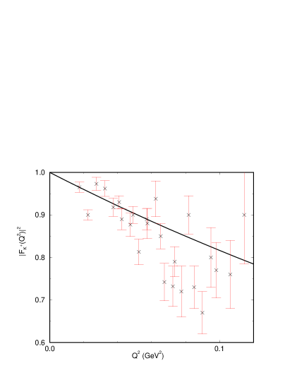
Figure 5.5: Kaon charge form factor from Burden, Roberts and Thomson (1996). The available data is shown and is from Amendolia et al. (1986b), and Dally et al.  (1980).

As discussed in Sec. 4.3, the underlying ladder BSE that is assumed here does not preserve the independence with respect to the partitioning parameter $\xi$ that would be a property of an exact treatment. The constraint imposed by Burden, Roberts and Thomson (1996) to fix $\xi$ is to require that the neutral kaon have exactly zero charge, i.e. $F_{K^{0}}(Q^{2}=0)=0$. This works in the following way. The generalized impulse approximation to the $K^{0}$ vertex is given by

$$\Lambda_{\mu}^{K^{0}}(P;Q)=(e_{d})\Lambda_{\mu}^{d}(P;Q)+(-e_{s})\bar{\Lambda}_{\mu}^{s}(P;Q)~{}.$$ (5.41)

The $u$ and $d$ quarks are taken as identical except for the electric charge and hence $\Lambda_{\mu}^{d}=\Lambda_{\mu}^{u}=\bar{\Lambda}_{\mu}^{u}$. If the $u$ and $s$ quark properties, except for the charge, are set equal in Eqs. (5.2) and (5.2) the generalised impulse approximation to the $\gamma\pi\pi$ vertex, Eq. (5.2), is recovered provided that $\Gamma_{K}\rightarrow\Gamma_{\pi}$, $f_{K}\rightarrow f_{\pi}$ and $\xi=1/2$, which is required by charge conjugation symmetry. This provides a consistency check. The same limit applied to Eq. (5.41) verifies the charge conjugation symmetry requirement that there is no photon coupling to the (self-conjugate) $\pi^{0}$. This formulation ensures EM current conservation because the quark-photon vertex satisfies the Ward identity and produces $F_{K^{\pm}}(Q^{2}=0)=1$. This happens because at $Q^{2}=0$ the generalized impulse approximation for the charged kaon vertex reduces to the normalization condition for the BS amplitude in a similar way that led to Eq. (5.2) for the pion. However for the non-self-conjugate $K^{0}$, there is not complete cancellation in Eq. (5.41) at $Q^{2}=0$ unless $\xi$ is suitably different from $1/2$ to counteract the different dynamics for the $d$ and $s$ quarks. The presence of this dependence reflects a deficiency of the ladder approximation to the BSE.

This formulation was applied by Burden, Roberts and Thomson (1996) using the Ball-Chiu Ansatz for $\Gamma_{\mu}$. The $u/d$ quark propagator parameters were fixed by pion physics and the only free parameters were the two $s$ quark parameters $C^{s}_{m_{s}=0}$ and $b^{s}_{2}$ described in Sec. 3. These parameters are determined by requiring that the model reproduce, as well as possible, the experimental values for the dimensionless quantities $f_{K}/f_{\pi}=1.22\pm 0.02$, $r_{K^{\pm}}/r_{\pi^{\pm}}=0.88\pm 0.07$ and $m_{K}/f_{K}=4.37\pm 0.05$. The ansatz

$$\Gamma_{K}(q;P^{2}=-m_{K}^{2})\approx i\gamma_{5}\,\frac{B_{m_{s}=0}^{s}(q^{2})}{f_{K}}~{},$$ (5.42)

is used with the associated kaon mass being obtained by solving $\hat{\Delta}^{-1}_{K}(P^{2})=0$, where the inverse propagator is as given in Eq. (4.25). The normalization constant is obtained from $f_{K}^{2}=\hat{\Delta}^{-1~{}\prime}_{K}(-m_{K}^{2})$ which also ensures the correct normalisation of the charged kaon form factor.

The obtained set of quark propagator parameters are those shown earlier in Table 3.1. The fit selects differences between the $u$ and $s$ quark propagators. The calculated electromagnetic form factor is reproduced in Fig. 5.5. The comparison between calculated and experimental pion and kaon quantities from tha work is presented in Table 3.2. For the neutral kaon $r^{2}_{K^{0}}<0$, and $F_{K^{0}}(Q^{2})$ is found to be similar in form and magnitude to the charge form factor of the neutron. The other quantities shown in Table 3.2 are obtained consistently from the same quark propagator model.

The difference between the calculated and measured values of the charge radii and scattering lengths in Table 3.2 is a measure of the importance of final-state, pseudoscalar rescattering interactions and photon–vector-meson mixing, which are not included in generalised-impulse approximation. The above calculation suggests that such effects contribute less than $\sim$ 15% and become unimportant for $Q^{2}>1$ GeV². The fact that the calculated values of $f_{K}/f_{\pi}$ and $r_{K}/r_{\pi}$ agree with the experimental values of these ratios suggests that such effects are no more important for the kaon than for the pion.

The results for $F(Q^{2})$ found by Burden, Roberts and Thomson (1996) for $K^{+}$ and $K^{0}$ at $Q^{2}<2$ GeV² are not sensitive to details of the propagator parametrization. Their qualitative features are similar to those from a recent quark loop investigation based on a separable interaction (Buck et al., 1995). However specific magnitudes are different. As is the case of the pion, the large $Q^{2}$ behavior is a faster fall-off than $1/Q^{2}$ due to both non-perturbative bound state amplitudes playing a role in this exclusive scattering process. The behavior of $F_{K^{\pm}}(Q^{2})$ at $Q^{2}>2\sim 3$ GeV² is influenced by details of the Ansatz for the kaon Bethe-Salpeter amplitude, Eq. (5.42), that are not presently constrained by data. This emphasizes that measurement of the electromagnetic form factors is a probe of the bound state structure of the meson and of non-perturbatively generated differences between the $u$ and $s$ quark propagators.

6 Meson Interactions

6.1 The $\pi^{0}\gamma\gamma$ Form Factor

The pion charge form factor for space-like momenta is one of the simplest but non-trivial testing grounds for applications of QCD to hadronic properties. A closely related quantity that has received less attention is the $\gamma^{*}\pi^{0}\rightarrow\gamma$ transition form factor (Ametller, Bijnens, Bramon and Cornet, 1992; Jaus, 1991). Here the photon momentum dependence maps out a particular off-shell extension of the axial anomaly (Adler, 1969; Bell and Jackiw, 1969). Presently available data for this transition form factor in the space-like region $Q^{2}<2.5$ GeV² is from the CELLO collaboration (Behrend et al., 1991) at the PETRA storage ring where the process $e^{+}e^{-}\rightarrow e^{+}e^{-}\pi^{0}$ was measured with geometry requiring one of the two intermediate photons to be almost real. There is renewed interest in this transition form factor due to the prospect of obtaining higher precision data over a broader momentum range via virtual Compton scattering from a proton target at CEBAF (Afanasev, 1994; Afanasev, Gomez and Nanda, 1994). The theoretical results (Frank et al., 1995) we summarize here can be viewed either as an application of the GCM model at the $0^{th}$ level of the meson loop expansion or as an application of the DSE approach truncated to generalized impulse approximation. The improvements over previous quark loop studies (Ito et al., 1992; Anikin et al., 1994) are: quark confinement (thus eliminating spurious quark production thresholds), dressing of the photon-quark vertex, and the dynamical relation between the pion Bethe-Salpeter amplitude and the quark propagator. The latter elements are crucial for producing the correct mass-shell axial anomaly independently of model details.

Using the action given in Eq. (5.21), the relevant interaction is generated by the first term $\hat{\cal S}_{1}[\pi;A]$. Expansion of the quark loop term shown as the first part of Eq. (5.22) yields

$${\cal S}[\pi^{0}\gamma\gamma]=-{\rm Tr}[S\;\Gamma_{\mu}A_{\mu}\;S\;\Gamma_{\nu}A_{\nu}\;S\;\Gamma_{\pi}\pi^{0}].$$ (6.1)

That is

$${\cal S}[\pi^{0}\gamma\gamma]=\int\frac{d^{4}Pd^{4}Q}{(2\pi)^{8}}A_{\mu}(-P-Q)A_{\nu}(Q)\pi^{0}(P)\Lambda_{\mu\nu}(P,Q),$$ (6.2)

where the vertex function is given by the integral

$$\Lambda_{\mu\nu}(P,Q)=-\mbox{tr}\int\frac{d^{4}k}{(2\pi)^{4}} S(k-P-Q)\Gamma_{\mu}(k-\mbox{\small$\displaystyle\frac{P}{2}$}-\mbox{\small$\displaystyle\frac{Q}{2}$};-P-Q)S(k)$$ (6.3)

$$\times\Gamma_{\nu}(k-\mbox{\small$\displaystyle\frac{Q}{2}$};Q)S(k-Q)\Gamma_{\pi}(k-\mbox{\small$\displaystyle\frac{P}{2}$}-Q;P).$$

Figure 6.1: The quark triangle diagram for the generalized impulse approximation to the $\gamma^{*}\pi^{0}\gamma$ vertex.

The momentum assignments are shown in the quark triangle diagram of Fig. 6.1. The general form of the vertex allowed by CPT symmetry is $\Lambda_{\mu\nu}(P,Q)=-i\frac{\alpha}{\pi f_{\pi}}\epsilon_{\mu\nu\alpha\beta}P_{\alpha}Q_{\beta}~{}g(Q^{2},P^{2},P\cdot Q)$ where $\epsilon_{4123}=1$, $\alpha$ is the fine-structure constant, $f_{\pi}$ is the pion decay constant, and $g$ is the off-mass-shell invariant amplitude. With the one photon mass-shell condition $(P+Q)^{2}=0$, the invariant amplitude, denoted by $g(Q^{2},P^{2})$, is the object of the calculation. For a physical pion the shape of the $\gamma^{*}\pi^{0}\rightarrow\gamma$ transition form factor is given by $g(Q^{2},-m^{2}_{\pi})$. The chiral limit for the physical $\pi^{0}\rightarrow\gamma\gamma$ decay amplitude is fixed at $\frac{\alpha}{\pi f_{\pi}}$ by the axial anomaly (Itzykson and Zuber, 1980) which gives an excellent account of the $7.7$ eV width and requires $g(0,0)=1/2$. This follows only from gauge invariance and chiral symmetry in quantum field theory and provides a stringent check upon model calculations.

In the work of Frank et al. (1995) the dressed photon-quark vertex $\Gamma_{\nu}$ is taken to be the Ball-Chiu Ansatz $\Gamma_{\nu}^{bc}$ from Eq. (5.27) and the pion BS amplitude is taken to be the $\gamma_{5}$ part $B(p^{2},m)/f_{\pi}$ as suggested by Eq. (4.9). The $\pi^{0}\gamma\gamma$ vertex function in Eq. (6.3) is now completely specified in terms of the quark propagator. An exactly parallel situation holds for the spacelike pion charge form factor produced from the same approach (Roberts, 1996) and discussed in Sec. 5.2. The parameters employed there are used without adjustment for $\pi\gamma\gamma$. At $Q^{2}=0$, numerical evaluation (Frank et al., 1995) yields $g_{\pi^{0}\gamma\gamma}=g(0,-m_{\pi}^{2})=0.496$, in agreement with the previous application of this model (Roberts, 1996) and in good agreement with the experimental value $0.504\pm 0.019$. The chiral limit of this approach has been shown (Roberts, 1996) to correctly incorporate the exact result $g(0,0)=1/2$ produced by the axial anomaly independent of the form and details of the quark propagator. This is only possible when all elements of the loop are dressed consistently as dictated by symmetries. Here this means the chiral limit $\gamma_{5}$ term of the pion BS amplitude is fixed by chiral symmetry through Eq. (4.9) in terms of the quark scalar self-energy amplitude, and the physical soft photon-quark vertex is fixed by EM gauge invariance through the Ward identity in terms of the quark propagator. It is advantageous to account for the distributed nature of pions and dressed quarks, not only because it is a realistic outcome of QCD, but also because important symmetries are implemented this way.

Figure 6.2: The $\gamma^{*}\pi^{0}\gamma$ transition form factor from Frank et al. (1995) along with the CELLO data from Behrend et al. (1991).

The obtained form factor $F(Q^{2})=g(Q^{2},-m_{\pi}^{2})/g(0,-m_{\pi}^{2})$ at the pion mass-shell is displayed as $Q^{2}F(Q^{2})$ in Fig. 6.2 by the solid line. A “radius” or interaction size, defined via $r^{2}_{\gamma\pi^{0}\gamma}=$ $-6\left.F^{\prime}(Q^{2})\right|_{Q^{2}=0}$, yields $0.47~{}{\rm fm}$ while a monopole fit to the data yields (Behrend et al., 1991) $0.65\pm 0.03~{}{\rm fm}$. The insert compares the low $Q^{2}$ result with a recent result from a QCD sum rule approach (Radyuskin, 1994), and a monopole form (Brodsky and Lepage, 1981) that interpolates from the leading asymptotic behavior $F(Q^{2})\rightarrow 8\pi^{2}f_{\pi}^{2}/Q^{2}$ argued from the pQCD factorization approach (Lepage and Brodsky, 1980). In the latter two approaches there is ambiguity due to: A) the unknown momentum scale at which perturbative behavior should set in; and B) assumptions for the pion wavefunction and how it should evolve with the momentum scale (Radyuskin, 1994). Within the present GCM/DSE approach, both the photon coupling and the pion wavefunction evolve with $Q^{2}$ in a way determined by the evolution of the dressed quark propagators. This produces, in a single expression, both the ultra-violet behavior required by pQCD and the infra-red limit dictated by the axial anomaly. We note from the parameterization of the quark propagator given in Eq. (3.28) and Eq. (3.29) that the employed pion Bethe-Salpeter amplitude $B(p^{2},m)/f_{\pi}$ has the correct leading power law behavior $m\lambda^{2}/p^{2}f_{\pi}$ which implements the hard gluon contribution that dominates pQCD.

The dotted straight line in Fig. 6.2 is the pQCD factorization (Lepage and Brodsky, 1980) limit $Q^{2}F(Q^{2})\rightarrow$ $8\pi^{2}f_{\pi}^{2}=0.67~{}{\rm GeV}^{2}$. Although the GCM/DSE non-factorized calculation reaches this value near $Q^{2}=$ $3~{}{\rm GeV}^{2}$, there is a slow decrease with higher $Q^{2}$ consistent with a logarithmic correction. An excellent fit to the numerical results for $3.3~{}{\rm GeV}^{2}\leq Q^{2}\leq 10~{}{\rm GeV}^{2}$ is provided by $F(Q^{2})=A~{}[1.0+$ $B~{}Q^{2}~{}\ln(C~{}Q^{2})]^{-1}$, where $A=1.021$, $B=0.461\,/m_{\rho}^{2}=0.777~{}{\rm GeV}^{-2}$ and $C=1.16\,/m_{\rho}^{2}=1.45~{}{\rm GeV}^{-2}$. (Neglected in this calculation is the anomalous dimension of the quark propagator; this would modify the power of the $\ln$-correction but would be a numerically small effect.)

The logarithmic correction to the anticipated $1/Q^{2}$ asymptotic behavior can be attributed to the persistent nonperturbative nature of the coupling to the final state soft photon in this exclusive process (Frank et al., 1995). Numerically it is found that, if a bare coupling were to be used for both photons as is implicit in the pQCD factorization approach, $F(Q^{2})$ would eventually approach $8\pi^{2}f_{\pi}^{2}/Q^{2}$. The turn-over in $Q^{2}F(Q^{2})$ near $3~{}{\rm GeV}^{2}$ predicted in Fig. 6.2 is barely within the $Q^{2}$ limit of $4~{}{\rm GeV}^{2}$ anticipated for measurements at CEBAF if a $6~{}{\rm GeV}$ electron beam becomes available. This turn-over and the logarithmic corrections generated by the loop integral are features also found in the parallel approach to the pion charge form factor (Roberts, 1996). For a study of the behavior of the vertex function off the pion mass shell, as needed for the anticipated CEBAF experiment, see Frank et al. (1995).

This $\pi\gamma\gamma$ approach has been recently extended without modification to the $\gamma\pi^{\ast}\rightarrow\pi\pi$ form factor (Alkofer and Roberts, 1996). The value $F^{3\pi}(4m_{\pi}^{2})$ of the amplitude at $s=4m_{\pi}^{2}$ from that work is shown in Table 3.2. This process is also due to the chiral anomaly and it is found, again, that the exact chiral limit current algebra result at the soft point $F^{3\pi}(0)=$ $eN_{c}/(12\pi^{2}f_{\pi}^{3})$ is produced independently of the details of consistently dressed elements of the loop. Together with the parallel result (Praschifka, Roberts and Cahill, 1987a) for the anomalous five-pion Wess-Zumino term, Eq. (4.35), these exact results from symmetries are produced at a truncated level of the theory. The correction terms, including meson loops, can apparently be absorbed into the details of the quark propagator dressing to which the chiral anomalies are evidently blind.

6.2 The $\rho\pi\pi$ Form Factor

From the second term of the action in Eq. (5.21), we identify ${\cal S}\left[\rho\pi\pi\right]=-{\rm Tr}\left[S\;\vec{\Gamma}_{\mu}^{\rho}\cdot\vec{\rho}_{\mu}\;(S\;\vec{\Gamma}_{\pi}\cdot\vec{\pi})^{2}\right]$, which yields

$${\cal S}\left[\rho\pi\pi\right]=i\int\frac{d^{4}P,Q}{(2\pi)^{8}}\vec{\rho}_{\mu}(Q)\cdot\vec{\pi}(-P-\mbox{\small$\displaystyle\frac{Q}{2}$})\times\vec{\pi}(P-\mbox{\small$\displaystyle\frac{Q}{2}$})\Lambda_{\mu}(P,Q)$$ (6.4)

where the vertex is

$$\Lambda_{\mu}(P,Q)=\int\frac{d^{4}k}{(2\pi)^{4}}V_{\rho}(k+\mbox{\small$\displaystyle\frac{P}{2}$};Q)E_{\pi}(k+\mbox{\small$\displaystyle\frac{Q}{4}$};-P-\mbox{\small$\displaystyle\frac{Q}{2}$})E_{\pi}(k-\mbox{\small$\displaystyle\frac{Q}{4}$};P-\mbox{\small$\displaystyle\frac{Q}{2}$})T_{\mu}(k,P,Q)$$ (6.5)

with

$$T_{\mu}(k,P,Q)=2N_{c}{\rm tr}_{s}\left[S(k+\mbox{\small$\displaystyle\frac{P}{2}$}+\mbox{\small$\displaystyle\frac{Q}{2}$})i\gamma_{\mu}^{T}S(k+\mbox{\small$\displaystyle\frac{P}{2}$}-\mbox{\small$\displaystyle\frac{Q}{2}$})i\gamma_{5}S(k-\mbox{\small$\displaystyle\frac{P}{2}$})i\gamma_{5}\right].$$ (6.6)

These expressions have been simplified through use of the approximations: only the $i\gamma_{5}\vec{\tau}E_{\pi}(q;P)$ part of the pion BS amplitude $\vec{\Gamma}_{\pi}$ has been used, and the $\rho$ BS amplitude $\vec{\Gamma}_{\mu}^{\rho}$ has been represented by $i\gamma_{\mu}^{T}\vec{\tau}V_{\rho}(q;Q)$ where $\gamma_{\mu}^{T}$ is transverse to the $\rho$ momentum $Q$. The $\rho\pi\pi$ vertex could have been obtained directly from the $\gamma\pi\pi$ vertex discussed in Sec. 5.2. Since only the isovector part ($\tau_{3}/2$) of $\hat{Q}$ from the photon-quark vertex contributes there, it is clear that the result for $\rho^{0}\pi\pi$ can be obtained by replacing $\Gamma_{\mu}/2$ for the photon with $i\gamma_{\mu}^{T}V_{\rho}(q;Q)$ for the $\rho^{0}$.

From symmetry properties, it is not difficult to show that $\Lambda_{\mu}(P,Q)=-\Lambda_{\mu}(-P,Q)=\Lambda_{\mu}(P,-Q)$, which requires the general form

$$\Lambda_{\mu}(P,Q)=-P_{\mu}\;F_{\rho\pi\pi}(P^{2},Q^{2},(P\cdot Q)^{2})-Q_{\mu}P\cdot Q\;H_{\rho\pi\pi}(P^{2},Q^{2},(P\cdot Q)^{2}).$$ (6.7)

With both pions on the mass-shell, $(P-\frac{Q}{2})^{2}=(P+\frac{Q}{2})^{2}=-m_{\pi}^{2}$. Equivalently, $P\cdot Q=0$ and $P^{2}=-m_{\pi}^{2}-\frac{Q^{2}}{4}$ so that only the first term of Eq. (6.7) survives. The corresponding form factor $F_{\rho\pi\pi}(Q^{2})$ contains the coupling constant as its mass-shell value, i.e. $F_{\rho\pi\pi}(Q^{2}=-m_{\rho}^{2})=g_{\rho\pi\pi}$. If the form factor is held at this triple mass-shell value independent of momenta, then Eq. (6.4), when converted to coordinate representation, becomes

$${\cal S}_{pt}\left[\rho\pi\pi\right]=-g_{\rho\pi\pi}\int d^{4}x\;\vec{\rho}_{\mu}(x)\cdot\vec{\pi}(x)\times\partial_{\mu}\vec{\pi}(x)~{},$$ (6.8)

which is the point coupling limit expressed in a standard form. There are, of course, other forms of action for this interaction that are on-shell equivalent. The general form of Eq. (6.4) is just one of them (in coordinate space it is a complicated non-local form). The momentum space form of Eq. (6.4) is an efficient way to account for the non-locality or off-shell structure of the interaction vertex produced by the quark-gluon substructure of the tree-level quantities within the GCM. One should bear in mind that the off-mass-shell behavior here in the meson momenta depends on what has been identified as the propagator for the $\bar{q}q$ meson modes as discussed in Sec. 2.2. It is always subject to a field redefinition and one must use a consistent definition throughout all elements used to construct an observable or S-matrix element.

Previous studies of the $\rho\pi\pi$ vertex within the GCM (Praschifka et al., 1987b; Roberts et al., 1988b; Hollenburg et al., 1992) made the approximation that $g_{\rho\pi\pi}$ could be estimated at the point $P=Q=0$. This was necessary to avoid ambiguities associated with numerical extrapolations of dressed quark propagators and vertex amplitudes in the integral Eq. (6.5). The parameterized analytic representation of the quark propagator described in Sec. 3 allows the correct mass-shell constraints to be maintained for $g_{\rho\pi\pi}$ and like quantities. Since the propagator parameters have so far been constrained only by pion physics, there is no guarantee that continuation of $S(p)$ away from the real $p^{2}$ axis by an amount proportional to $m_{\rho}^{2}$ will be correct. The exploratory calculations involving vector mesons described here constitute a first investigation of this matter.

Figure 6.3: The $\rho\pi\pi$ form factor versus $\rho$ momentum from Mitchell and Tandy, (1997).

The $\rho\pi\pi$ vertex has recently been studied within the GCM/DSE approach by Tandy (1996) and also by Mitchell and Tandy (1997). Those works use $E_{\pi}(q;P)=B(q^{2},m)/f_{\pi}$ and the parameterization $\Gamma^{\rho}(p^{2})\propto e^{-p^{2}/a^{2}}$. The strength is set by the canonical normalization condition given in Eq. (2.61). The range $a$ is then adjusted to reproduce the empirical value $g_{\rho\pi\pi}^{\rm expt}=6.05$. This approach has proved to be phenomenologically successful for studies of other processes such as $\rho-\omega$ mixing (Mitchell et al., 1994) and the $\rho\rightarrow e^{+}\;e^{-}$ decay (Pichowshy and Lee, 1996) from essentially the same theoretical framework. The produced $\rho\rightarrow\pi\pi$ decay width, given by

$$\Gamma_{\rho\rightarrow\pi\pi}=\frac{g_{\rho\pi\pi}^{2}}{4\pi}\frac{m_{\rho}}{12}\left[1-\frac{4m_{\pi}^{2}}{m_{\rho}^{2}}\right]^{3/2},$$ (6.9)

is $151~{}{\rm MeV}$. The calculated form factor $F_{\rho\pi\pi}(Q^{2})$ is shown in Fig. 6.3 for timelike and spacelike momenta in the vicinity of the mass-shell at $-0.6~{}{\rm GeV}^{2}$ indicated by a dot. The main conclusion from this calculation is that the previous approximation of using zero momentum to extract a coupling constant (Praschifka et al., 1987b) can underestimate the value by almost a factor of $2$.

These investigations are exploratory in the sense that an independent calculation of the $\rho$ BS amplitude $\Gamma_{\rho}(p)$ has not been employed. There are indications that an improved parameterization of $V_{\rho}(p^{2})$ to include a more realistic power-law fall-off at high momenta provides a simultaneous accounting for both $\rho\rightarrow\pi\pi$ and $\rho\rightarrow e^{+}\;e^{-}$ decays (Roberts, 1997). Covariants other than the canonical one $\gamma_{\mu}^{T}$ for the $\rho$ BS amplitude can contribute to the $\rho\pi\pi$ vertex and this has recently been investigated together with the effect of the sub-dominant pion covariants (Qian and Tandy, 1997). Truncation to the dominant $\rho$ amplitude is found to be an accurate approximation while the effect of the pseudoscalar pion component can be quite important.

The strong suppression displayed in Fig. 6.3 as $Q^{2}$ increases from the mass-shell point to the spacelike region indicates that the effective coupling strength $g_{\rho\pi\pi}(Q^{2})$ appropriate to the $\rho$ contribution to the pion charge form factor and radius is significantly smaller than what is assumed in the standard VMD approach. This is consistent with findings discussed in Sec. 5.2. The strong dependence in Fig. 6.3 is very similar to that found recently (Frank and Roberts, 1996) in a study that used a $\rho$ amplitude from solution of the BSE. In that work the time-like region of the form factor could not be calculated directly because the numerical solution of the $\rho$ BSE was performed only on the real $q^{2}>0$ axis. The results there suggest that the common procedure (e.g. see Eq. (56) of Frank and Roberts (1996)) of interpolation of calculated form factors in the meson momentum from the Euclidean domain to the mass-shell point can be reliable if the mass is not too large.

6.3 The $\gamma\pi\rho$ Form Factor

The empirical $\rho$ BS amplitude set by $g_{\rho\pi\pi}$ as above enables a parameter-free prediction for the $\gamma\pi\rho$ vertex. Apart from being a consistency check in this manner, the $\gamma\pi\rho$ interaction together with the $\gamma\pi\pi$, $\gamma\gamma\pi$, and the $\rho\pi\pi$ processes, provide important guidance for extending the present approach for nonperturbative QCD modeling of meson physics beyond phenomena dictated by chiral symmetry. Within nuclear physics, the associated isoscalar $\gamma^{*}\pi\rho$ meson-exchange current contributes significantly to electron scattering from light nuclei at presently available momenta. In particular, our understanding of the deuteron EM structure functions for $Q^{2}\approx 2-4~{}{\rm GeV}^{2}$ is presently hindered by uncertainties in the behavior of this form factor (Ito and Gross, 1993).

Figure 6.4: The $\gamma\pi\rho$ form factor versus photon momentum from Mitchell (1995) and Tandy (1996).

Expansion of the second term of the action in Eq. (5.21) to first order in the EM field yields the $\gamma\pi\rho$ interaction as the pair of contributions

$${\cal S}[\gamma\pi\rho]=-{\rm Tr}[S\;\Gamma_{\mu}A_{\mu}S\;\vec{\Gamma}_{\pi}\cdot\vec{\pi}\;S\;\vec{\Gamma}_{\nu}^{\rho}\cdot\vec{\rho}_{\nu}]-{\rm Tr}[S\;\Gamma_{\mu}A_{\mu}\;S\;\vec{\Gamma}_{\nu}^{\rho}\cdot\vec{\rho}_{\nu}\;S\;\vec{\Gamma}_{\pi}\cdot\vec{\pi}].$$ (6.10)

With a vertex function $\Lambda_{\mu\nu}(P,Q)$ defined by

$${\cal S}[\gamma\pi\rho]=-\int\frac{d^{4}P,Q}{(2\pi)^{8}}\;A_{\nu}(Q)\;\vec{\pi}(-P-\mbox{\small$\displaystyle\frac{Q}{2}$})\cdot\vec{\rho}_{\mu}(P-\mbox{\small$\displaystyle\frac{Q}{2}$})\;\Lambda_{\mu\nu}(P,Q),$$ (6.11)

one may combine the two terms in Eq. (6.10) to obtain the integral

$$\Lambda_{\mu\nu}(P,Q) = \mbox{\small$\displaystyle\frac{e}{3}$}\int\frac{d^{4}k}{(2\pi)^{4}}E_{\pi}(k+\mbox{\small$\displaystyle\frac{Q}{4}$};-P-\mbox{\small$\displaystyle\frac{Q}{2}$})V_{\rho}(k-\mbox{\small$\displaystyle\frac{Q}{4}$};P-\mbox{\small$\displaystyle\frac{Q}{2}$})$$ (6.12)

$$\times 2N_{c}{\rm tr}_{s}\big{[}S(k_{+}-\mbox{\small$\displaystyle\frac{Q}{2}$})\Gamma_{\nu}(k_{+};Q)S(k_{+}+\mbox{\small$\displaystyle\frac{Q}{2}$})i\gamma_{5}S(k_{-})i\gamma_{\mu}^{T}\big{]}~{}.$$

Here $k_{\pm}=k\pm\frac{P}{2}$. The approximations made here for the $\pi$ and $\rho$ BS amplitudes are identical to those used for the $\rho\pi\pi$ interaction in Sec. 6.2. Use of the Ward-Takahashi identity from Eq. (5.8) in Eq. (6.12) shows that in this formulation the $\gamma\pi\rho$ EM current is conserved, that is $Q_{\nu}\;\Lambda_{\mu\nu}(P,Q)=0$. The general form of the vertex function can be shown by symmetries to be

$$\Lambda_{\mu\nu}(P,Q)=-i\frac{e}{m_{\rho}}\;\epsilon_{\mu\nu\alpha\beta}\;P_{\alpha}Q_{\beta}~{}g_{\rho\pi\gamma}~{}f(Q^{2},P^{2},P\cdot Q)~{},$$ (6.13)

as is expected for a coupling arising from the chiral anomaly. We have used the standard definition of the coupling constant so that, at the triple mass-shell point, the form factor $f=1$.

The coupling constant and form factor resulting from the GCM or DSE approach truncated to the level shown above have been obtained by Mitchell (1995) and by Tandy (1996). The form of the quark propagator parameterization is that discussed in Sec. 3 and the Ball-Chiu Ansatz is used for $\Gamma_{\nu}$. Those works obtain $g_{\gamma\pi\rho}=0.5$ The experimental $\rho^{+}\rightarrow\pi^{+}\gamma$ partial width ($67\pm 7~{}{\rm keV}$) determines the empirical value $g_{\gamma\pi\rho}^{\rm expt}=0.54\pm 0.03$. The $\gamma\pi\rho$ form factor obtained with on-mass-shell $\pi$ and $\rho$, and weighted by $Q^{2}$, is shown by the solid curve in Figure 6.4. Also shown is the form factor suggested by vector meson dominance (VDM) as initially used to treat such meson exchange effects in electron scattering analysis (Hummel and Tjon, 1990), as well as the result from a free constituent quark loop with bare photon coupling (Ito and Gross, 1993; Ito et al., 1992). Both quark-based approaches produce a much softer form factor than does the VDM assumption. Above $50~{}{\rm fm}^{-2}$, which is readily accessible in electron scattering, the differences are serious. Since this calculation for $\gamma\pi\rho$ is equivalent to the $0^{th}$ term in the meson loop expansion. An estimate of meson-loop corrections to this result would be interesting.

7 Beyond Meson Tree Level

The essence of the GCM approach is that the tree-level meson fields are ladder $\bar{q}q$ bound states whose structure and interactions are governed by what we might call their dressed quark core. Further quantum treatment will generate meson loop effects from integration over these fields. That is the dressing of ladder mesons by ladder mesons. This extends the bound state structure of the mesons to add meson cloud effects to the original dressed quark core. In the more general DSE approach, such processes are implemented by use of less severe truncations of the equations of motion; also exposed that way in the DSE approach will be contributions from explicit gluon $n$-point functions that are not already accounted for by dressed quarks and mesons. In either case, it is clear that the approach just outlined is out of practical reach if one has to proceed too far into the loop expansion or with higher $n$-point functions to capture the dominant low energy physics. A crucial question then is the size of meson loop contributions to the various processes of interest, such as those observables we have described in previous Sections. In the GCM/DSE approach, the composite and extended structure of the tree-level meson fields makes such investigations difficult. On the other hand, the distributed vertex functions for the coupling tend to suppress the numerical importance of the meson dressing loop integrals, and it might be spectulated that for this approach the meson loops play much less of a role than for point coupling models or for effective field theories built from point coupling of point interpolating meson fields. We shall review the few investigations that have tackled this question in the GCM/DSE approach. Besides the pion loop contribution to the pion charge form factor, we also include here a discussion of vector meson mode contributions to this quantity.

7.1 Role of Vector Mesons in the Pion Form Factor

The relative unimportance of the $\rho$ for the space-like pion charge form factor in the present quark-gluon approach is consistent with considerations of vector-meson–photon mixing in QCD. It can be understood in terms of Eq. (5.16) which is the dressed photon-quark vertex $\Gamma_{\nu}$ separated into a $\rho$ pole term and a non-resonant or direct background term. With both terms of that vertex employed for coupling to the pion in the manner discussed in Sec. 5.2, one obtains

$$F_{\pi}(Q^{2})=F_{\pi}^{GIA}(Q^{2})+\frac{F_{\rho\pi\pi}(Q^{2})\;\Pi^{\rho\gamma}_{T}(Q^{2})}{Q^{2}+m_{\rho}^{2}(Q^{2})}~{}.$$ (7.1)

The first term is from the non-resonant photon vertex term and is the generalized impulse approximation (GIA) that we have described in Sec. 5.2. The second term is the $\rho$ resonant term that arises in the GCM or DSE approaches. The relative importance of the two terms away from the $\rho$ mass-shell depends strongly upon their momentum dependence. The off-mass-shell momentum behavior of individual terms in photon vertex separations such as $\Gamma_{\nu}=\Gamma_{\nu}^{nr}+\Gamma_{\nu}^{pole}$, given in Eq. (5.16), and that underly Eq. (7.1), will differ in different approaches. The total result should not.

In the naive limit of a point coupling model with structureless hadrons, the elements of Eq. (7.1) become $F_{\pi}^{GIA}(Q^{2})\rightarrow 1$, $F_{\rho\pi\pi}(Q^{2})\rightarrow g_{\rho\pi\pi}$, and $\Pi^{\rho\gamma}_{T}(Q^{2})\rightarrow-Q^{2}/g_{V}$. The latter $Q^{2}$ factor arises from the description of the mixing as proportional to $\int d^{4}x\rho_{\mu\nu}(x)\;F_{\mu\nu}(x)$. This produces the VMD empirical form

$$F_{\pi}(Q^{2})=1-\frac{g_{\rho\pi\pi}\;Q^{2}}{g_{V}\,(Q^{2}+m_{\rho}^{2})}~{}.$$ (7.2)

where the first (contact) term accounts for the pion charge and the charge radius is required to come totally from the second ($\rho$ propagator) term. This implies $r_{\pi}^{2}\sim 6g_{\rho\pi\pi}/(m_{\rho}^{2}g_{V})$, which under the universality assumption of vector coupling $g_{V}\approx g_{\rho\pi\pi}$, produces $r_{\pi}^{2}\sim 0.4~{}{\rm fm}^{2}$ which compares very well with the experimental value $0.44~{}{\rm fm}^{2}$. In this sense it is often considered that the spacelike pion charge form factor is the tail of the $\rho$ resonance. A recent re-examination of the VMD phenomenology for this and related processes with two choices of point hadron lagrangian can be found in the work of O’Connell et al., (1995). We note that the phenomenological form (VMD1) found preferable there obeys the massless photon constraint $\Pi^{\rho\gamma}_{T}(0)=0$ and produces just the point limit in Eq. (7.2). We also note that the more standard form of VMD, called VMD2 by O’Connell et al., (1995), uses universal vector coupling and also the assumption that $\Pi^{\rho\gamma}_{T}(Q^{2})\approx m_{\rho}^{2}/g_{V}$ for all $Q^{2}$; then the equivalence of Eq. (7.2) to $m_{\rho}^{2}/(m_{\rho}^{2}+Q^{2})$ is often used to invoke the extreme form of VMD, namely that the photon couples only through vector mesons.

From the perspective of the GCM or DSE approaches, the reality of a space-time distributed quark-gluon substructure of the pions, for example, demands the distributed form for the form factor shown in Eq. (7.1) rather than the point form in Eq. (7.2). These considerations certainly apply also to QCD. The question of the relative importance of the two terms in Eq. (7.1) then arises. This will receive different answers in different formulations for it depends on how the separation is defined off-mass-shell. This corresponds to the observation that there is no unique way to separate a pole contribution from a background contribution except precisely at the pole. The sum of the two terms is the meaningfull quantity. With adoption of the Ball-Chiu Ansatz, this representation of the non-resonant term of the photon-quark vertex shares with the BSE vertex those aspects of momentum dependence that are constrained by symmetries including the Ward-Takahashi identity. Since the vector mesons are described by the same kernel, it should not be surprizing that at least some extrapolation of vector $\bar{q}q$ correlations into the spacelike region is accounted for through the Ball-Chiu vertex. A similarity in strength between the Ball-Chiu vertex and the spacelike extension of low mass vector meson poles has recently been found (Frank, 1995) through a numerical study of the ladder BSE for the photon vertex. It is quite a robust result that about $85-90$% of the experimental value of $r_{\pi}$ is produced by the resulting non-resonant or generalized impulse term in the work of Roberts (1996); the value of $f_{\pi}r_{\pi}$ is quite insensitive to variation in the representation of the dressed quark propagator if other constaints such as $m_{\pi}$ and $\langle\bar{q}q\rangle$ are maintained.

This leads to considerations of why the $\rho$ contribution should be small in such an approach. There is a constraint at $Q^{2}=0$. Electromagnetic gauge invariance requires the $\rho$-$\gamma$ mixing amplitude $\Pi^{\rho\gamma}_{T}(Q^{2})$, and hence the pole term of $F_{\pi}(Q^{2})$ in Eq. (7.1), to vanish at $Q^{2}=0$. Asymptotic freedom ensures $\Pi^{\rho\gamma}_{T}(Q^{2})$ vanishes at large spacelike-$Q^{2}$; hence a small contribution to $F_{\pi}(Q^{2})$ from the $\gamma\rho$ mixing term over a large range of space-like $Q^{2}$ can be consistent. A more detailed investigation requires a consistent definition of the momentum dependence of the separation in Eq. (5.16) as related to the $\rho$ BS amplitude and the defined non-resonant photon vertex. An initial investigation has utilized a mass-shell BS amplitude for the $\rho$-meson which is well described as a $\bar{q}q$ bound state within the ladder BS approach; such a dressed-quark core gives $\sim$ 90% of its mass (Hollenburg, Roberts and McKellar, 1992; Burden, Qian, Roberts, Tandy and Thomson, 1996). A calculation (Roberts, 1996) based on this confirms that $\Pi^{\rho\gamma}_{\mu\nu}(Q^{2})$ is a slowly varying function for spacelike $Q^{2}$. The momentum suppression of the pole term of Eq. (7.1) due to $F_{\rho\pi\pi}(Q^{2})$ is quite strong as discussed in Sec. 6.2 and displayed in Fig. 6.3. We may use the representations $F_{\rho\pi\pi}(Q^{2})=g_{\rho\pi\pi}f_{\rho\pi\pi}(Q^{2})$ and $\Pi^{\rho\gamma}_{T}(Q^{2})=-Q^{2}\hat{f}_{\rho\gamma}(Q^{2})/g_{V}$, where the two new functions $f$ and $\hat{f}$ depend on the details of the dynamics. The $\rho$ pole contribution to the pion charge radius from Eq. (7.1) can then be written in the form

$$(r_{\pi}^{pole})^{2}=r_{\pi}^{2}-(r_{\pi}^{GIA})^{2}=1.2\;f_{\rho\pi\pi}(0)\hat{f}_{\rho\gamma}(0)\;\frac{6}{m_{\rho}^{2}}~{},$$ (7.3)

where we have used the empirical result $g_{\rho\pi\pi}/g_{V}\sim 1.2$. Since from Fig. 6.3 $f_{\rho\pi\pi}(0)\approx 0.5$, one estimates that a value $\hat{f}_{\rho\gamma}(0)\approx 0.4$ would account for all of the difference between the non-resonant $(r_{\pi}^{GIA})^{2}$ in Table 3.2 ($0.31~{}{\rm fm}^{2}$) and the experimental value ($0.44~{}{\rm fm}^{2}$). A reasonable value $\hat{f}_{\rho\gamma}(0)\approx 0.3$ would leave room for a contribution as well from the pion loop process of the size estimated by Alkofer et al.(1995) and described below.

7.2 Pion Loop Shift of the $\rho$ Mass

At the tree level of the GCM, the ladder description of the $\rho$ and $\omega$ is degenerate, $m_{\rho}=m_{\omega}$. The pion loop correction to the $\rho$ self-energy produces a mass shift and also a width due to the open $2\pi$ channel. Within the GCM, this mass shift was originally studied by Hollenburg et al.(1992). We review the later work on the shift and width by Mitchell and Tandy (1997) and highlight some issues that generally arise in the GCM or DSE approaches.

Mitchell and Tandy (1997) treat the transverse $\rho$ and $\omega$ modes and use fields that contain the transverse projector $T_{\mu\nu}(P)=\delta_{\mu\nu}-P_{\mu}P_{\nu}/P^{2}$. That is, $\vec{\rho}_{\mu}(P)\equiv T_{\mu\nu}(P)\vec{\rho}_{\nu}(P)$ and $\omega_{\mu}(P)\equiv T_{\mu\nu}(P)\omega_{\nu}(P)$. In a matrix notation where $V_{\mu}$ denotes $(\vec{\rho}_{\mu},\omega_{\mu})$, the tree-level action from Eq. (2.63), up to second order in the fields, can be written as

$$\hat{S}_{2}[\rho,\omega]=\mbox{\small$\displaystyle\frac{1}{2}$}\int\frac{d^{4}P}{(2\pi)^{4}}V^{T}_{\mu}(-P)\Bigl{[}\hat{\Delta}^{-1}_{\mu\nu}(P)+\hat{\Pi}_{\mu\nu}^{q}(P)\Bigr{]}V_{\nu}(P).$$ (7.4)

Here, in meson channel space, $\hat{\Delta}^{-1}$ is diagonal and the only non-zero elements of $\hat{\Pi}^{q}$ are the off-diagonal ones that provide $\rho^{0}-\omega$ coupling via the $u-d$ current mass difference. The superscript $q$ identifies the quark-loop contribution to distinguish from subsequent pion loop quantities. The composite $\bar{q}q$ nature of the mesons is reflected in the fact that the diagonal inverse propagators contain a dynamical mass function. The general form

$$\hat{\Delta}^{-1}(P^{2})\,=\,(P^{2}+m_{V}^{2}){\cal Z}_{1}^{-1}(P^{2})\,=\,(P^{2}+m_{V}^{2}(P^{2}))$$ (7.5)

as calculated from the formalism in Sec. 2.2 identifies the degenerate mass $m_{V}$ of the tree-level $\rho$ and $\omega$ states. The momentum dependence of ${\cal Z}_{1}(P^{2})$ is due to the $\bar{q}q$ substructure. Without $\rho^{0}-\omega$ mixing, a physical normalization (unit residue at the mass-shell pole) would be produced by absorbing at least the on-mass-shell value of ${\cal Z}_{1}^{-\frac{1}{2}}$ into the fields. The function ${\cal Z}_{1}^{-\frac{1}{2}}(P^{2})$ may be absorbed into the fields producing unmixed propagators have the standard point meson form. As in Sec. 2.2 the associated BS amplitudes become correspondingly rescaled as $\Gamma_{V}(q;P)=\hat{\Gamma}_{V}(q;P)~{}{\cal Z}_{1}^{\frac{1}{2}}(P^{2})$, so that at the mass-shell the standard normalization condition (Itzykson and Zuber, 1980) is satisfied.

The relevant low-order terms in the effective action for $\pi,\rho,\omega$ from the bosonization result in Eq. (2.64) are

$$\hat{S}\left[\pi,\rho,\omega\right]=\hat{S}_{2}\left[\rho,\omega\right]+\hat{S}_{2}\left[\pi\right]+\hat{S}[\rho\pi\pi]+\hat{S}[\omega\pi\pi]+\cdots.$$ (7.6)

Here the quadratic terms $\hat{S}_{2}\left[\rho,\omega\right]$ and $\hat{S}_{2}[\pi]$ represent respectively the $\rho-\omega$ sector containing the quark-loop mixing mechanism and the free pion sector. To integrate out the pion fields, it is convenient to first combine the last three terms of Eq. (7.6) so that it becomes

$$\hat{S}\left[\pi,\rho,\omega\right]=\hat{S}\left[\rho,\omega\right]+\mbox{\small$\displaystyle\frac{1}{2}$}\int\frac{d^{4}P,P^{\prime}}{(2\pi)^{8}}\,\pi_{i}(P^{\prime})D^{-1}_{ij}(P^{\prime},P)\pi_{j}(P).$$ (7.7)

The three terms in

$$D_{ij}^{-1}(P^{\prime},P)=\Delta^{-1}_{ij}(P^{\prime},P)+V_{ij}(P^{\prime},P)+W_{ij}(P^{\prime},P)$$ (7.8)

correspond to the tree-level pion inverse propagator given by

$$\Delta^{-1}_{ij}(P^{\prime},P)=(2\pi)^{4}\delta_{ij}\delta^{4}(P^{\prime}+P)\Delta^{-1}_{\pi}(P^{2}),$$ (7.9)

the $\rho\pi\pi$ interaction term given by

$$V_{ij}(P^{\prime},P)=2i\epsilon_{ijk}\,\rho_{\mu}^{k}(-P^{\prime}-P)\;\Lambda_{\mu}^{\rho}(-\frac{P^{\prime}+P}{2};-P^{\prime}-P),$$ (7.10)

and the $\omega\pi\pi$ interaction term given by

$$W_{ij}(P^{\prime},P)=2i\epsilon_{ij3}\,\omega_{\mu}(-P^{\prime}-P)\;\Lambda_{\mu}^{\omega}(-\frac{P^{\prime}+P}{2};-P^{\prime}-P).$$ (7.11)

In this work the pion inverse propagator of the GCM is reduced to the standard point form by absorbing the calculated ${\cal Z}_{\pi}^{-\frac{1}{2}}(P^{2})$ into the pion field. Thus the pion momentum dependence of the $\rho\pi\pi$ and $\omega\pi\pi$ vertex functions contain the compensating aspects of the $\bar{q}q$ substructure of the pion. The $\rho\pi\pi$ vertex function is described in Sec. 6.2. The corresponding $\omega\pi\pi$ vertex function, which is generated by a $u-d$ current quark mass difference, is calculated and included by Mitchell and Tandy (1997) to extract the pion loop contribution to $\rho-\omega$ mixing. Integration over the pion fields allows a new effective action $\hat{{\cal S}}[\rho,\omega]$ to be identified from

$$Z=N\int D\rho D\omega D\pi\,{\rm exp}\left(-\hat{S}[\pi,\rho,\omega]\right)=N^{\prime}\int D\rho D\omega\,{\rm exp}\left(-\hat{{\cal S}}[\rho,\omega]\right)$$ (7.12)

by using the functional integral result

$$\int D\pi\,{\rm exp}\left(-\mbox{\small$\displaystyle\frac{1}{2}$}\int\frac{d^{4}P,P^{\prime}}{(2\pi)^{8}}\,\pi_{i}(P^{\prime})D^{-1}_{ij}(P^{\prime},P)\pi_{j}(P)\right)={\rm exp}\left(-\mbox{\small$\displaystyle\frac{1}{2}$}{\rm TrLn}\;D^{-1}\right).$$ (7.13)

The field-independent term ${\rm exp}(-\frac{1}{2}{\rm TrLn}\;\Delta^{-1})$ from the result may be absorbed into the normalization constant to arrive at

$$\hat{{\cal S}}\left[\rho,\omega\right]=\hat{S}_{2}\left[\rho,\omega\right]+\mbox{\small$\displaystyle\frac{1}{2}$}{\rm TrLn}(1+\Delta(V+W)).$$ (7.14)

The second term here gives the vector meson coupling to all orders produced by a single pion loop.

Figure 7.1: The real and imaginary parts of the pion loop contribution to the $\rho$ self-energy. Taken from Mitchell and Tandy (1997).

The quadratic part of the second term of Eq. (7.14) adds a contribution to the tree-level $\rho^{0}-\omega$ matrix inverse propagator. The net transverse result is

$${\cal D}^{-1}(P^{2})=\left(\begin{array}[]{cc}P^{2}+m_{V}^{2}+\Pi^{\rho\rho}(P^{2})&\Pi^{\rho\omega}(P^{2})\\ \Pi^{\rho\omega}(P^{2})&P^{2}+m_{V}^{2}+\Pi^{\omega\omega}(P^{2})\end{array}\right),$$ (7.15)

where the net mixing amplitude is $\Pi^{\rho\omega}(P^{2})=\Pi^{q}(P^{2})+\Pi^{\pi}(P^{2})$. The additional terms produced by the pion loop are the diagonal self-energies $\Pi^{\rho\rho}(P^{2})$ and $\Pi^{\omega\omega}(P^{2})$, and the mixing term $\Pi^{\pi}(P^{2})$. From Eq. (7.14), the self-energy contribution $\Pi^{\rho\rho}(P^{2})$ is given by the transverse component of

$$\Pi^{\rho\rho}_{\mu\nu}(P)=-4\int\frac{d^{4}q}{(2\pi)^{4}}\Delta_{\pi}(q_{+})\Delta_{\pi}(q_{-})\Lambda^{\rho}_{\mu}(q;-P)\Lambda^{\rho}_{\nu}(q;P),$$ (7.16)

where $q_{\pm}=q\pm P/2$, and the summation over pion isospin labels has been carried out. This contribution is the same for each isospin component of the $\rho$. The $\omega$ self-energy contribution is obtained from Eq. (7.16) by the replacement of $\Lambda^{\rho}$ by $\Lambda^{\omega}$. It is quadratic in the small symmetry breaking mechanism and is ignored.

In the absence of mixing, the real part of $~{}\Pi^{\rho\rho}(P^{2})$ generates a mass shift for the isospin eigenstate $\rho_{I}$. This mass shift now represents the $\rho-\omega$ mass splitting. For timelike momenta such that $P^{2}\leq-4m_{\pi}^{2}$, both $~{}\Pi^{\rho\rho}(P^{2})$ and $~{}\Pi^{\pi}(P^{2})$ have imaginary parts associated with the decay $\rho\rightarrow 2\pi$. This mechanism should produce most of the $\rho$ width. The mass modifications due to mixing are second order in a very small quantity and are ignored. The shifted $m_{\rho}$ is therefore identified from the position of the zero in the real part of the relevant inverse propagator in Eq. (7.15). That is,

$$m_{\rho}^{2}=m_{\omega}^{2}+{\rm Re}\,\Pi^{\rho\rho}(-m_{\rho}^{2}),$$ (7.17)

where now $m_{\omega}=m_{V}$. With the definition $\hat{\Gamma}(P^{2})=-{\rm Im}\,\Pi^{\rho\rho}(P^{2})/m_{\rho}$, the inverse propagator in the $\rho$ channel can be written as

$${\cal D}^{-1}_{\rho}(P^{2})=(P^{2}+m_{\rho}^{2}-im_{\rho}\Gamma(P^{2}))\,{\cal Z}_{2}^{-1}(P^{2}),$$ (7.18)

where $\Gamma(P^{2})=\hat{\Gamma}(P^{2})~{}{\cal Z}_{2}(P^{2})$. The function ${\cal Z}_{2}(P^{2})$ arises from the momentum dependence of the real part of the pion loop self-energy. The on-mass-shell value, which is the $\rho$ field renormalization constant due to the $2\pi$ content, is given by

$${\cal Z}_{2}^{-1}(-m_{\rho}^{2})=1+{\rm Re}\,{\Pi^{\rho\rho}}^{\prime}(-m_{\rho}^{2}),$$ (7.19)

with the prime superscript denoting differentiation with respect to the argument. One absorbs ${\cal Z}_{2}^{-\frac{1}{2}}(P^{2})$ into the field $\rho_{\mu}(P)$ so that the resulting propagator has the conventional Breit-Wigner form. The physical width is given by

$$\Gamma_{\rho}=-m_{\rho}^{-1}\,{\cal Z}_{2}(-m_{\rho}^{2})\,{\rm Im}\,\Pi^{\rho\rho}(-m_{\rho}^{2}).$$ (7.20)

Figure 7.2: Graphical determination of the $\rho-\omega$ mass difference due to the pion loop. The influence of the $\bar{q}q$ composite nature of the $\pi$ and $\rho$ propagators is also shown. Taken from Mitchell and Tandy (1997).

Numerical results for the $\rho$ mass shift and width are obtained from Eq. (7.16) in the specific form (Mitchell and Tandy, 1997)

$$\Pi^{\rho\rho}(P^{2})=-\frac{4}{3}f_{\rho\pi\pi}^{2}(P^{2})\int\frac{d^{4}q}{(2\pi)^{4}}\frac{(q^{2}-(q\cdot P)^{2}/P^{2})e^{-2q^{2}/\lambda_{\rho}^{2}(P^{2})}}{\left[(q+\frac{P}{2})^{2}+m_{\pi}^{2}-i\epsilon\right]\left[(q-\frac{P}{2})^{2}+m_{\pi}^{2}-i\epsilon\right]},$$ (7.21)

where a parameterized form of the calculated $\rho\pi\pi$ vertex function is used for convenience. The numerical results for ${\rm Re}\,\Pi^{\rho\rho}(P^{2})$ and ${\rm Im}\,\Pi^{\rho\rho}(P^{2})$ are shown in Fig. 7.1. The self-consistent solution for $m_{\rho}$ produced by Eq. (7.17) is displayed in Fig. 7.2 in the following way. The quantity $-(P^{2}+m_{\omega}^{2})$ is plotted as a long dash line and its intercept with the solid line representing ${\rm Re}\,\Pi^{\rho\rho}(P^{2})$ identifies the mass shell point. With $m_{\omega}=m_{V}=782~{}{\rm MeV}$ one finds $m_{\rho}=761~{}{\rm MeV}$ giving $m_{\rho}-m_{\omega}=-21~{}{\rm MeV}$. The experimental value is $-12.0\pm 0.8$ MeV. The calculated width is $\Gamma_{\rho}=156~{}{\rm MeV}$ while the experimental value is $151~{}{\rm MeV}$. Fig. 7.2 also illustrates the contribution to the mass splitting result made by the momentum dependence of the meson self-energies generated by the $\bar{q}q$ substructure. This is most marked for the pion and enters the pion loop integral in Eq. (7.16) through the factors ${\cal Z}_{\pi}(q_{\pm}^{2})$ which are contributed by each pion propagator. (In the calculational procedure these factors have been moved into the vertex functions for convenience.) If each function ${\cal Z}_{\pi}$ is held constant at its mass-shell value (as would be the case for a structureless pion), the full calculation in Fig. 7.2 (solid line) becomes the dot-dashed line. The intercept then indicates that the mass shift would be essentially zero. In contrast to this, the short dashed line indicates that the influence of the corresponding quantity ${\cal Z}_{1}(P^{2})$, from the $\bar{q}q$ substructure of the $\rho$, is quite negligible here. This is because the range of variation in $P^{2}$ is very small.

Figure 7.3: The pion charge form factor. The first term is the generalized impulse approximation, and the second term is the one pion loop correction. Double lines represent the ladder $\bar{q}q$ pions of the GCM/DSE approach. Quark lines are dressed propagators and circles are dressed vertices.

7.3 Pion Loop Part of the Pion Charge Radius

A somewhat more complicated task is presented by the pion loop contribution to the pion charge radius. This is illustrated in Fig. 7.3. The analysis has been carried out within the GCM framework by Alkofer, Bender and Roberts (1995) in the following way. Starting from the tree level GCM meson action of Eq. (5.25), which includes coupling to a background EM field, the first-order contributions in the pion loop expansion may be developed for various vertex functions. For the $\gamma\pi\pi$ vertex function, Alkofer et al., (1995) obtain

$$\Lambda_{\mu}(P;Q)=\Lambda_{\mu}^{GIA}(P;Q)+\Lambda_{\mu}^{loop}(P;Q)~{},$$ (7.22)

where the first term is the generalized impulse approximation result (i.e., at meson tree level) given by Eq. (5.2) and discussed in Sec. 5.2. The pion loop contribution is given by

$$\epsilon^{3ij}\;\Lambda_{\mu}^{loop}(P;Q)=-\mbox{\small$\displaystyle\frac{1}{2}$}\int\frac{d^{4}K}{(2\pi)^{4}}T^{ijkl}(Q,P-K,K+P)\;\Delta_{\pi}(K_{+})\Delta_{\pi}(K_{-})\;\epsilon^{3kl}\;\Lambda_{\mu}^{GIA}(K;Q)~{},$$ (7.23)

where $K_{\pm}=K\pm Q/2$ and $T^{ijkl}((p_{1},p_{2};p_{3},p_{4})$ is the $\pi-\pi$ scattering kernel which may be written in terms of a single invariant amplitude $A(p_{1},p_{2};p_{3},p_{4})$. A threshold expansion for this amplitude in low powers of momentum is not adequate here since the integral in Eq. (7.23) samples a large domain of spacelike momenta. The contribution to the required $A(p_{1},p_{2};p_{3},p_{4})$ that yields both the leading order chiral limit result at low $s$, the term (Weinberg, 1966) given in Eq. (4.36), and the leading contribution within the GCM at tree level for large $s$, is obtained from the action in Eq. (4.33) in the form

$$\hat{{\cal S}}_{R}[U]=\int d^{4}xd^{4}y\;\mbox{\small$\displaystyle\frac{f_{\pi}^{2}}{2}$}{\rm tr}\left[\partial_{\mu}U(x)\partial_{\mu}U(y)^{\dagger}\right]\hat{f}(x-y)~{},$$ (7.24)

which avoids the derivative expansion by retaining the nonlocality. Here $\hat{f}(x-y)$ is the fourier transform of the momentum space quark loop integral with two chiral insertions. It is of the same form that contributes to the pion inverse propagator as discussed in Sec. 4.1.

For the integral in Eq. (7.23), the onshell approximation $\Lambda_{\mu}^{GIA}(K;Q)\approx 2K_{\mu}F_{\pi}^{GIA}(Q^{2})$ is made. The result is expressed in the form

$$F_{\pi}(Q^{2})=F_{\pi}^{GIA}(Q^{2})\left[1+L(Q^{2};m_{\pi})\right]~{},$$ (7.25)

where $L$ is a result from the pion loop integral. Since the condition $F_{\pi}(0)=1$ is equivalent to the proper normalization condition for the pion BS amplitude, the above form emphasises that the pion loop mechanism generates additional internal structure for the pion. A renormalization of the modified BS amplitude is necessary. The form $i\gamma_{5}B(q^{2})/f_{\pi}$ used at each $\pi\bar{q}q$ vertex is now effectively supplemented by an additional pion cloud term. The normalization constant $f_{\pi}$, previously determined at the quark loop level, must be renormalized to adjust for the pion cloud now being included in the pion. From these considerations, Alkofer et al., (1995) report results in the form

$$r_{\pi}^{2}=(r_{\pi}^{GIA})^{2}+(r_{\pi}^{loop})^{2}$$ (7.26)

where the first-order pion loop contribution $r_{\pi}^{loop}(m_{\pi})$ is at most $10-15$% of the generalized impulse approximation (meson tree-level) result. The loop term has the expected divergence as a chiral logarithm in the $m_{\pi}\rightarrow 0$ limit, but it has the stated small effect at the physical point and is seen to not dominate until $m_{\pi}\sim 10~{}{\rm MeV}$. The pion loop correction to $f_{\pi}$ is found to be at most $2$% of the impulse or tree-level result.

In ChPT with $N_{f}=3$, the result given by Gasser and Leutwyler (1985) up to one pseudoscalar loop is

$$r_{\pi}^{2}=\frac{12\,L^{r}_{9}}{f_{\pi}^{2}}-\frac{1}{32\pi^{2}\,f_{\pi}^{2}}\left[2\;{\rm ln}\left(\frac{m_{\pi}^{2}}{\mu^{2}}\right)+{\rm ln}\left(\frac{m_{K}^{2}}{\mu^{2}}\right)+3\right]~{},$$ (7.27)

where $L^{r}_{9}$ is the $9^{th}$ low energy constant at ${\cal O}(p^{4})$ after the divergent part from the loop has been absorbed and $\mu^{2}$ is the loop regularization scale. Any reasonable choice of $\mu^{2}$ such as $m_{\rho}^{2}$, leads to the “chiral logarithms” in Eq. (7.27) contributing typically $15$% of the experimental value $0.44~{}{\rm fm}^{2}$. The dominant $L^{r}_{9}$ term is the counterpart in ChPT of $(r_{\pi}^{GIA})^{2}$ obtained from the distributed quark-gluon substructure of the $\gamma\pi\pi$ vertex in the GCM/DSE approaches. However the correspondence is only approximate; the distinction between tree-level and loops in the two approaches is not the same due to the very different character of the pseudoscalar fields. This has been discussed in the early part of Sec. 4.2.

8 Concluding Remarks

We have summarized the Global Color Model as it applies to a variety of meson physics observables. A constant theme that emerges is that the tree level interactions among $\bar{q}q$ Goldstone mesons and photons are well-described in terms of only the dressed quark propagators. This efficiency is due to the connection between the pseudoscalar Bethe-Salpeter amplitudes and the quark propagator brought about by chiral symmetry and also by the connection between the photon-quark vertex and the propagator brought about by electromagnetic gauge invariance. Only tentative steps have been taken so far in the task of relating the phenomenological aspects of the confining quark propagators used at this stage to an underlying gluon $2$-point function. This step is required if the GCM is to fulfil the initially designed role of a field theory model based upon an effective gluon $2$-point function. This need is emphasized by investigations of mesons other than the Goldstone bosons where more approximations must necessarily be made. However, even with an increased degree of phenomenological input, valuable information is being obtained.

We have seen that various coupling constants obtained at meson tree-level are within $10$% of experiment. At that stage the meson modes from the GCM have ladder Bethe-Salpeter content and the meson coupling is via a dressed quark loop. An interesting question is whether this will be a persistent theme that leaves meson loop corrections relatively unimportant in this approach. This is possible because the subsequent meson loop dressing would have to overcome distributed coupling caused by the finite size effects of the tree-level mesons in this approach. There are only several isolated pieces of evidence. Pion-loop corrections to the pion EM form factor were seen to contribute at the level of $<15$% to the charge radius (Alkofer et al., 1995). Similarly, the pion-loop contribution to the downward shift in the $\rho$ mass relative to $m_{\omega}$ in the GCM has been found to be $<5$% (Hollenburg et al., 1992) and in a more recent study $2$% (Mitchell and Tandy, 1997); this latter result is in good agreement with experiment. It would certainly be a convenience if the low-mass mesons and their soft interactions were amenable to a representation in which their dressed quark content captures the dominant quantum loop effects. However this remains to be determined and in this regard future work within the GCM is called for to obtain the pion loop contributions to the $\pi-\pi$ scattering lengths especially $a_{0}^{0}$. In ChPT at ${\cal O}(p^{4})$, the only distributed substructure enters through loops of the (auxiliary) point pion fields, while at tree level in the GCM there is significant substructure through all orders in momenta. A systematic comparison through a complete set of threshold observables at ${\cal O}(p^{4})$ would be quite useful. One of the features of the GCM is that constraints from asymptotic freedom at large momenta are automatically included and the complete momentum dependence of form factors and scattering processes can be examined. From this perspective, one may speculate that with a model field theory with a few parameters such as the GCM, high accuracy in threshold behavior might be incompatible with quality descriptions of many processes over a large momentum domain. More work is needed to explore a large variety of observables.

There has been significant effort in the past devoted to investigations of baryons (particularly the nucleon) within a covariant Faddeev formalism truncated to a quark-diquark approximation derived within the GCM. Probably the first covariant Faddeev calculation of the nucleon (Burden, Cahill and Praschifka, 1989) was carried out within the GCM framework. Other works (Cahill, Roberts and Praschifka, 1987; 1989a; Praschifka et al., 1989) have made important contributions to understanding the properties and role of diquarks as constituents of baryons. Progress in this endeavour is complicated by the rich singularity structure of the covariant Faddeev equations. A more accessible, but necessarily more approximate approach to the nucleon has been via chiral meson-quark mean field models of the non-topological soliton variety. The GCM has provided a definitive underpinning to such methods by producing the soliton equations of motion for these degrees of freedom as dressed composite modes based at the quark level (Cahill and Roberts, 1985; Frank, Tandy and Fai, 1991). As a confining quark condensate model of the nucleon it has provided very efficient and sensible numerical results (Frank and Tandy, 1992). Space has not permitted an analysis of such baryon work to be included here.

References

Afanasev, A. (1994). Form factors of the transitions $\gamma^{\ast}\pi^{0}\rightarrow\gamma$ and $\gamma^{\ast}\pi^{0}\rightarrow\gamma$, Proc. of the Workshop on CEBAF at Higher Energies, CEBAF, Newport News, Eds. N. Isgur and P. Stoler, P. 185; Afanasev, A., Gomez, J. and Nanda, S. (1994). CEBAF Letter of Intent # LOI-94/005, unpublished.

Adler, S. (1969). Axial-vector in spinor electrodynamics, Phys. Rev. 177, 2426.

Alkofer, R., Bender, A. and Roberts, C.D. (1995). Pion loop contribution to the electromagnetic pion charge radius, Int. J. Mod. Phys. A 10, 3319.

Alkofer, R. and Roberts, C.D. (1996). Calculation of the anomalous $\gamma\pi^{\ast}\rightarrow\pi\pi$ form factor. Phys. Lett. B 369, 101.

Amendolia, S.R., et al. (1986a). A measurement of the spacelike pion electromagnetic form-factor, Nucl. Phys. B 277, 168.

Amendolia, S.R., et al. (1986b). A measurement of the kaon charge radius, Phys. Lett. B 178, 435.

Ametller, L., Bijnens, L., Bramon, A. and Cornet, F. (1992). Transition form-factors in $\pi^{0}$, $\eta$ and $\eta^{\prime}$ couplings to $\gamma\gamma$, Phys. Rev. D 45, 986.

Anikin, I. V., Ivanov, M. A., Kulimanova N. B. and Lyubovitskij, V. E. (1994). Sensitivity to form-factors in the extended Nambu–Jona-Lasinio model with separable interactions, Sov. J. Nucl. Phys. 57, 1082.

Aoki, Ken-Ichi, Kugo, Taichiro and Mitchard, Mark K. (1991). Meson properties from the ladder Bethe-Salpeter equation, Phys. Lett. B 266, 467.

Ball, J.S. and Chiu, T.-W. (1980). Analytic properties of the vertex function in gauge theories. I and II, Phys. Rev. D, 22, 2542.

Barducci, A., Casalbuoni, R., De Curtis, S., Dominici, D and Gatto, R. (1988). Dynamical chiral-symmetry breaking and determination of the quark masses, Phys. Rev. D 38, 238.

Bar-Gadda, U. (1980). Infrared behavior of the effective coupling in quantum chromodynamics, Nucl. Phys. B 163, 312.

Bebek, C. J., et al.(1976). Determination of the pion form factor up to $Q^{2}=4~{}{\rm GeV}^{2}$ from single charged-pion electroproduction, Phys. Rev. D 13, 25.

Bebek, C. J., et al.(1978). Electroproduction of single pions at low $\epsilon$ and a measurement of the pion form factor up to $Q^{2}=10~{}{\rm GeV}^{2}$, Phys. Rev. D 17, 1693.

Behrend, H.J., et al. (CELLO Collab.), (1991). A measurement of the $\pi^{0}$, $\eta$ and $\eta^{\prime}$ electromagnetic form factors, Z. Phys. C 49, 401.

Bell, J. and Jackiw, R. (1969). A PCAC puzzle: $\pi^{0}$ to $\gamma\;\gamma$ in the sigma-model, Nuovo Cimento A60, 47.

Bender, A., Roberts, C.D. and v. Smekal, L. (1996). Goldstone theorem and diquark confinement beyond rainbow-ladder approximation, Phys. Lett. B 380, 7.

Bernard, C., Parrinello, C. and Soni, A. (1994). A lattice study of the gluon propagator in momentum space, Phys. Rev. D 49, 1585.

Bernard, V., Brockmann, R. and Weise, W. (1985). The Goldstone pion and the quark anti-quark pion. II. Pion size and decay, Nucl.Phys. A 440, 605.

Bernard, V. and Meißner, U.-G. (1988). Electromagnetic structure of the pion and the kaon, Phys. Rev. Lett. 61, 2296.

Bernard, V., Kaiser, N. and Meißner, U.-G. (1995). Chiral dynamics in nucleons and nuclei, Int. J. Mod. Phys. E 4, 193.

Blin, A.H., Hiller, B. and Schaden, M. (1988). Electromagnetic form-factors in the Nambu–Jona-Lasinio model, Z. Phys. A. 331, 75.

Brodsky, S.J. and Lepage, G.P. (1981). Large-angle two-photon exclusive channels in quantum chromodynamics, Phys. Rev. D 24, 1808.

Brown, C. N., et al., (1973). Coincidence electroproduction of charged pions and the pion form factor, Phys. Rev. D 8, 92.

Brown, N. and Pennington M.R. (1988a), Preludes to confinement: Infrared properties of the gluon propagator in the Landau gauge, Phys. Lett. B 202, 257.

Brown, N. and Pennington, M. (1988b). Studies of confinement: How quarks and gluons propagate, Phys. Rev. D 38, 2266.

Brown, N. and Pennington, M.R. (1989). Studies of confinement: How the gluon propagates, Phys. Rev. D 39, 2723.

Buck, A., Alkofer, R. and Reinhardt, H. (1992). Baryons as bound states of diquarks and quarks in the Nambu–Jona-Lasinio model, Phys. Lett. B 286, 29.

Buck, W.W., Williams, R.A. and Ito, H. (1995). Elastic charge form factors for $K$ mesons, Phys. Lett. B 351, 24.

Burden, C.J., Cahill, R.T. and Praschifka, J. (1989). Baryon structure and QCD: Nucleon calculations, Aust. J. Phys. 42, 147.

Burden, C.J. and Roberts, C.D. (1991). Light-cone regular vertex in three-dimensional quenched QED, Phys. Rev. D 44, 540.

Burden, C.J., Praschifka, J. and Roberts, C.D. (1992a). Photon polarization tensor and gauge dependence in three-dimensional quantum electrodynamics, Phys. Rev. D 46, 2695.

Burden, C.J. and Roberts, C.D. (1993). Gauge covariance and the fermion-photon vertex in three-dimensional and four-dimensional, massless quantum electrodynamics, Phys. Rev. D 47, 5581.

Burden, C.J., Roberts, C.D. and Williams, A.G. (1992). Singularity structure of a model quark propagator, Phys. Lett. B 285, 347.

Burden, C.J., Roberts, C.D. and Thomson, M. J. (1996). Electromagnetic Form Factors of Charged and Neutral Kaons, Phys. Lett. B 371, 163.

Burden, C.J., Qian, Lu, Roberts, C.D., Tandy, P.C. and Thomson, M.J. (1997). Ground state spectrum of light-quark mesons, Phys. Rev. C 55, 2649.

Burkardt, M., Frank, M.R. and Mitchell, K.L. (1997). Calculation of hadron form factors from Euclidean Dyson-Schwinger equations, Phys. Rev. Lett. 78, 3059.

Cahill, R.T. and Roberts, C.D. (1985). Soliton bag models of hadrons from QCD, Phys. Rev. D 32, 2419.

Cahill, R.T., Roberts, C.D. and Praschifka, J. (1987). Calculation of diquark masses in QCD, Phys. Rev. D 36, 2804.

Cahill, R.T., Roberts, C.D. and Praschifka, J. (1989a). Baryon structure and QCD, Aust. J. Phys. 42, 129.

Cahill, R.T., Praschifka, J. and Burden, C.J. (1989b). Diquarks and the bosonization of QCD, Aust. J. Phys. 42, 161.

Cahill, R.T. (1989). Hadronization of QCD, Aust. J. Phys. 42, 171.

Cahill, R.T. (1992). Hadronic laws from QCD, Nucl. Phys. A 543, 63.

Cahill, R.T. (1993). Private communication.

Cahill, R.T. and Gunner, S. (1995a). Quark and gluon propagators from meson data, Phys. Lett. B 359, 281.

Cahill, R.T. and Gunner, S. (1995b). A new mass formula for NG bosons in QCD, Mod. Phys. Lett. B 10, 3051.

Cahill, R.T. and Gunner, S. (1997). The global color model of QCD and its relationship to the NJL model, chiral perturbation theory and other models, Aust. J. Phys. 50, 103.

Celenza, L.S., Shakin, C.M., Sun, W.-D., Szweda, J. and Zhu, X. (1995). Quark model calculations of current correlators in the nonperturbative domain, Ann. Phys. (N.Y.) 241, 1.

Celenza, L.S., Shakin, C.M. and Sun, W.-D. (1996). Calculation of the nucleon-nucleon interaction due to vector-meson exchange, Phys. Rev. C 54, 487.

Curtis, D.C. and Pennington, M.R. (1992). Generating fermion mass in quenched QED in four-dimensions, Phys. Rev. D 46, 2663.

Dally, E.B., et al. (1980). Direct measurement of the negative kaon form factor, Phys. Rev. Lett. 45, 232.

Delbourgo, R. and Scadron M.D. (1979). Proof of the Nambu-Goldstone realisation for vector-gluon–quark theories, J. Phys. G 5, 1621.

Dong, Z., Munczek, H.J. and Roberts, C.D. (1994). Gauge covariant fermion propagator in quenched, chirally-symmetric quantum electrodynamics, Phys. Lett. B 333, 536.

Donoghue, J.F., Golowich, E. and Holstein, B.R. (1992). Dynamics of the Standard Model, Cambridge University Press.

Ebert, D. and Reinhardt, H. (1986). Effective chiral hadron Lagrangian with anomalies and Skyrme terms from quark flavor dynamics, Nucl. Phys. B 271, 188.

Ecker, G. (1996). Low-energy QCD, Prog. Part. Nucl. Phys. 36, 71.

Efimov, G.V and Ivanov, M.A. (1993). The Quark Confinement Model of Hadrons, IOP Publishing, Bristol.

Eguchi, T. and Sugawara H. (1974). Extended model of elementary particles based on an analogy with superconductivity, Phys. Rev. D 10, 4257.

Eguchi, T. (1976). A new approach to collective phenomena in superconductivity models, Phys. Rev. D 14, 2755.

Frank, M.R. (1995). Nonperturbative aspects of the quark-photon vertex, Phys. Rev. C 51, 987.

Frank, M.R. and Meissner, T. (1996). Low-energy QCD: chiral coefficients and the quark-quark interaction, Phys. Rev. C 53, 2410.

Frank, M. R., Mitchell, K. L., Roberts, C. D. and Tandy, P. C. (1995). The off-shell axial anomaly via the $\gamma^{\ast}\pi^{0}\rightarrow\gamma$ transition, Phys. Lett. B 359, 17.

Frank, M.R. and Tandy, P.C. (1992). Confining quark condensate model of the nucleon, Phys. Rev. C 46, 338.

Frank, M.R., Tandy, P.C. and Fai, G. (1991). Chiral solitons with quarks and composite mesons, Phys. Rev. C 43, 2808.

Frank, M.R. and Roberts, C.D. (1996). Model gluon propagator and pion and rho meson observables, Phys. Rev. C 53, 390.

Frank, M.R. and Tandy, P.C. (1994). Gauge invariance and the electromagnetic current of composite pions, Phys. Rev. C 49, 478.

Gasser, J. and Leutwyler, H. (1982). Quark masses, Phys. Rep. 87, 77.

Gasser, J. and Leutwyler, H. (1983). Low energy theorems as precision tests of QCD, Phys. Lett. B 125, 325.

Gasser, J. and Leutwyler, H. (1984). Chiral perturbation theory to one loop, Ann. Phys. (N.Y.) 158, 142.

Gasser, J. and Leutwyler, H. (1985). Chiral perturbation theory: Expansions in the mass of the strange quark, Nucl. Phys. B 250, 465; 517; 539.

Gasser, J. (1995). The $\pi\pi$ scattering amplitude in chiral perturbation theory, $DA\Phi NE$ Physics Handbook, $2^{nd}$ Ed., Eds. L. Maiani, G. Pancheri and N. Paver, P. 215.

Gell-Mann, M., Oakes, R. and Renner, B. (1968). Behavior of current divergences under SU(3) $\otimes$ SU(3), Phys. Rev. 175, 2195.

Gross, F. and Milana, J. (1994). Goldstone pion and other mesons using a scalar confining interaction, Phys. Rev. D 50, 3332.

Hawes, F. T. and Williams, A. G. (1995). Chiral symmetry breaking in quenched massive strong-coupling four-dimensional QED, Phys. Rev. D 51, 3081.

Hollenberg, L.C.L., Roberts, C.D. and McKellar, B.H.J. (1992). Two loop calculation of the $\omega$-$\rho$ mass splitting, Phys. Rev. C 46, 2057.

Hubbard, J. (1959). Calculation of partition functions, Phys. Rev. Lett. 3, 77.

Hummel, E. and Tjon, T.J. (1990). Relativistic analysis of meson exchange currents in elastic electron deuteron scattering, Phys. Rev. C 42, 423.

Ito, H., Buck, W. W. and Gross, F. (1992). The axial anomaly and the dynamical breaking of chiral symmetry in the $\gamma^{\ast}\pi^{0}\rightarrow\gamma$ reaction, Phys. Lett. B287, 23

Ito, H. and Gross, F. (1993). Isoscalar meson exchange currents and the deuteron form-factors, Phys. Rev. Lett. 71, 2555.

Itzykson C. and Zuber, J.-B. (1980). Quantum Field Theory. McGraw-Hill, New York.

Jackiw, R. and Johnson, K. (1973). Dynamical model of spontaneously broken gauge symmetries, Phys. Rev. D 8, 2386.

Jain, P. and Munczek, H.J. (1993). $q\bar{q}$ bound states in the Bethe-Salpeter formalism, Phys. Rev. D 48, 5403.

Jaus, W. (1991). Relativistic constituent quark model of electroweak properties of light mesons, Phys. Rev. D 44, 2851.

Kikkawa, K. (1976). Quantum corrections in superconductor models, Prog. Theor. Phys. 56, 947.

Kleinert, H. (1976a). Quark masses, Phys. Lett. B 62, 77.

Kleinert, H. (1976b). Hadronization of quark theories and a bilocal form of QED, Phys. Lett. B 62, 429.

Kleinert, H. (1978). Hadronization of Quark Theories, Proceedings of the 1976 School of Subnuclear Physics, Erice, Ed. A. Zuihuchi, (Plenum).

Klevansky, S.P. (1992). The Nambu–Jona-Lasinio model of quantum chromodynamics, Rev. Mod. Phys. 64, 649.

Kugo, T. (1978). Dynamical instability of the vacuum in the Lagrangian formalism of the Bethe-Salpeter bound states, Phys. Lett. B 76, 625.

Kusaka, K. and Williams, A. G. (1995). Solving the Bethe-Salpeter equation for scalat theories in Minkowski space, Phys. Rev. D 51, 7026.

Langfeld, K., Kettner, C. and Reinhardt, H. (1996). A renormalizable extension of the NJL-model, Nucl. Phys. A 608, 331.

Leinweber, D. B. and Cohen, T. D. (1993). Chiral corrections to lattice calculations of charge radii, Phys. Rev. D 47, 2147.

Lepage, G.P. and Brodsky, S.J. (1980). Exclusive processes in perturbative quantum chromodynamics, Phys. Rev. D 22, 2157.

Le Yaouanc, A., Oliver, L., Ono, S., Pene, O., and Raynal, J. C. (1985). A quark model of light mesons with dynamically broken chiral symmetry, Phys. Rev. D 31, 137.

Llewellyn-Smith, C. H. (1969). A relativistic formulation of the quark model for mesons, Ann. Phys. (N.Y.) 53, 521.

Marciano, W. and Pagels, H. (1978). Quantum chromodynamics. Phys. Rep. C 36 137.

Maris, P. and Holties H. (1992). Determination of the singularities of the Dyson-Schwinger equation for the quark propagator, Intern. J. Mod. Phys A 7, 5369.

McKay, D. and Munczek, H.J. (1985). Anomalous chiral Lagrangians of pseudoscalar, vector, and axial-vector mesons generated from quark loops, Phys. Rev. D 32, 266.

McKay, D., Munczek, H.J. and Young, B.-L., (1989). From QCD to the low-energy effective action through composite fields: Goldstone’s theorem and $f_{\pi}$, Phys. Rev. D 37, 195.

Meissner, T. (1994). The convergence radius of the chiral expansion in the Dyson-Schwinger approach, Phys. Lett. B 340, 226.

Meissner, T. (1997). The mixed quark-gluon condensate from an effective quark-quark interaction, preprint, hep-ph/9702293.

Meißner, U.-G. (1993). Recent developments in chiral perturbation theory, Rep. Prog. Phys. 56, 903.

Miransky, V.A. (1990). On the wave function of light pseudoscalar mesons, Mod. Phys. Lett. A 5, 1979.

Mitchell, K.L. (1995). Meson dynamics from a QCD model field theory, Ph.D. Dissertation, Kent State University, unpublished.

Mitchell, K.L. and Tandy, P.C. (1997). Pion loop contribution to $\rho-\omega$ mixing and mass splitting, Phys. Rev. C 55, 1477.

Mitchell, K.L., Tandy, P.C., Roberts, C.D. and Cahill, R.T. (1994). Charge symmetry breaking via $\rho-\omega$ mixing from model quark-gluon dynamics, Phys. Lett. B 335, 282.

Molzon, W.R., et al. (1978). K(S) regeneration of electrons from 30-GeV/c to 100-GeV/c: A measurement of the K0 radius, Phys. Rev. Lett. 41, 1213.

Munczek, H.J. and Nemirovsky, A.M. (1983). Ground-state $q\bar{q}$ mass spectrum in quantum chromodynamics, Phys. Rev. D 28, 181.

Munczek, H.J. and Jain. P. (1992). Relativistic pseudoscalar $q\bar{q}$ bound states: Results on Bethe-Salpeter wavefunctions and decay constants, Phys. Rev. D 46, 438.

Nambu, Y. and Jona-Lasinio, G. (1961). Dynamical model of elementary particles based on an analogy with superconductivity. I., Phys. Rev. 122, 345.

Narison, S. (1989). QCD Spectral Sum Rules, (World Scientific, Singapore).

O’Connell, H.B., Pearce, B.C., Thomas, A.W. and Williams, A.G. (1994). Constraints on the momentum dependence of rho-omega mixing, Phys. Lett. B 336, 1.

O’Connell, H.B., Pearce, B.C., Thomas, A.W. and Williams, A.G. (1995). Rho-Omega mixing and the pion electromagnetic form factor, Phys. Lett. B 354, 14.

Pagels, H. and Stokar, S. (1979). Pion decay constant, electromagnetic form factors, and quark electromagnetic self-energy in quantum chromodynamics, Phys. Rev. D 20, 2947.

Particle Data Group (1996). Review of Particle Physics, Phys. Rev. D 54, 1.

Pichowsky, M.A. and Lee, T.-S.H. (1996). Pomeron exchange and exclusive electroproduction of $\rho$-mesons in QCD, Phys. Lett. B 379, 1.

Pocanć, D. Chiral Dynamics: Theory and Experiment, Eds. A.M. Bernstein and B.R. Holstein, Lecture Notes in Physics, 452, p. 95 (Springer, Berlin, 1995)

Politzer, H. D. (1982). Effective quark masses in the chiral limit, Nucl. Phys. B 117, 397.

Praschifka, J., Roberts, C.D. and Cahill, R.T. (1987a). QCD bosonization and the meson effective action, Phys. Rev. D 36, 209.

Praschifka, J., Roberts, C.D. and Cahill, R.T. (1987b). A Study of $\rho\rightarrow\pi\pi$ Decay in a Global Colour Model for QCD, Intern. J. Mod. Phys. A 2, 1797.

Praschifka, J., Cahill, R.T. and Roberts, C.D. (1989). Mesons and diquarks in chiral QCD: Generation of constituent quark masses, Intern. J. Mod. Phys. A 4, 4929.

Qian, Lu. and Tandy, P.C. (1997). In preparation.

Radyushkin, A.V. (1994). Nonperturbative QCD and elastic processes at CEBAF energies, Proc. of the Workshop on CEBAF at Higher Energies, CEBAF, Newport News, Eds. N. Isgur and P. Stoler, P.273.

Reinders, L.J., Rubinstein, H. and Yazaki, S. (1985). Hadron properties from QCD sum rules, Phys. Rep. 127, 1.

Reinhardt, H. (1990). Hadronization of quark flavor dynamics, Phys. Lett. B 244, 316.

Roberts, C.D. (1996). Electromagnetic pion form factor and neutral pion decay width, Nucl. Phys. A 605, 475.

Roberts, C.D. (1997). Private communication.

Roberts, C.D. and Cahill, R.T. (1987). A Bosonisation of QCD and Realisations of Chiral Symmetry, Aust. J. Phys. 40, 499.

Roberts, C.D., Cahill, R.T. and Praschifka, J. (1988). The effective action for the Goldstone modes in a global colour symmetry model of QCD, Ann. Phys. (N.Y.) 188, 20.

Roberts, C.D., Cahill, R.T. and Praschifka, J. (1988b). QCD and a calculation of the omega-rho mass splitting, Int. J. Mod. Phys. A 4, 719.

Roberts, C.D., Praschifka, J. and Cahill, R.T. (1989). A chirally symmetric effective action for vector and axial vector fields in a global colour symmetry model of QCD, Intern. J. Mod. Phys. A 4, 1681.

Roberts, C.D. and McKellar, B.H.J. (1990). Critical coupling for dynamical chiral symmetry breaking, Phys. Rev. D 41, 672.

Roberts, C.D and Williams, A.G. (1994). Dyson-Schwinger equations and their application to hadronic Physics, Prog. Part. Nucl. Phys. 33, 477, Ed. A. Fäßler (Pergamon Press, Oxford, 1994).

Roberts, C.D., Williams, A.G. and Krein, G. (1992). On the implications of confinement, Intern. Journal Mod. Phys. A 7, 5607.

Roberts, C.D., Cahill, R.T., Sevior, M.E., Iannella, N. (1994). $\pi$-$\pi$ scattering in a QCD based model field theory, Phys. Rev. D 49, 125.

Rothe, H.J. (1992). Lattice Gauge Theories: An Introduction, Lecture Notes in Physics, Vol. 43. World Scientific, Singapore.

Sakurai, J.J. (1969). Currents and Mesons, University of Chicago Press.

Shakin, C.M. and Sun, W.-D. (1997). Microscopic foundations of the vector meson dominance model and the analysis of rho-omega mixing, Phys. Rev. D 55, 2874.

Shrauner, E. (1977). Bilocal fields for the study of quantum corrections to dynamically broken symmetries, Phys. Rev. D 16, 1887.

Sommerer, A.J., Spence, J.R. and Vary, J. P. (1994). Relativistic momentum space wave equations and meson spectroscopy, Phys. Rev. C 49, 513.

Stainsby, S.J. and Cahill, R.T. (1992). The analytic structure of quark propagators, Int. J. Mod. Phys. A, 7, 7541.

Stratonovich, R.L. (1957). On a method of calculating quantum distribution functions, Sov. Phys. Dokl. 2, 416.

Tandy, P.C. (1996). Meson transition form factors from a QCD model field theory, Prog. Part. Nucl. Phys. 36 97.

Tandy, P.C. (1997). in preparation.

Takahashi, Y. (1957). On the generalised Ward identity. Nuovo Cimento 6, 370.

Van Orden, J.W., Devine, N. and Gross, F. (1995). Elastic electron scattering from the deuteron using the Gross equation. Phys. Rev. Lett. 75, 4369.

Vogl, U. and Weise, W. (1991). The Nambu and Jona-Lasinio model: its implications for hadrons and nuclei, Prog. Part. Nucl. Phys. 27, 195.

Volkov, M. K. (1984). Meson lagrangians in a superconductor quark model. Ann. Phys. (N.Y.) 157, 282.

Volkov, M. K. and Ebert, D. (1982). Four-quark interactions as a common dynamical basis of the $\sigma$ model and the vector dominance model. Sov. J. Nucl. Phys. 36, 736.

Ward, J.C. (1950). An identity in quantum electrodynamics. Phys. Rev. 78, 182.

Weinberg, S. (1966). Pion scattering lengths, Phys. Rev. Lett. 17, 616.

Wess, J. and Zumino, B. (1971). Consequences of anomalous ward identities, Phys. Lett. B 37, 95.

Wick, G.C. (1954). Properties of the Bethe-Salpeter wavefunctions, Phys. Rev. 96, 1954.

Williams, A.G., Krein, G. and Roberts, C.D. (1991). Modelling the quark propagator, Ann. Phys. (N.Y.) 210, 464.

Witten, E. (1979). Current algebra theorems for the U(1) Goldstone Boson, Nucl. Phys. B 156, 269.