Halo Excitation of ⁶He in Inelastic and Charge-Exchange Reactions

Abstract

Four-body distorted wave theory appropriate for nucleon-nucleus reactions leading to 3-body continuum excitations of two-neutron Borromean halo nuclei is developed. The peculiarities of the halo bound state and 3-body continuum are fully taken into account by using the method of hyperspherical harmonics. The procedure is applied for $A=6$ test-bench nuclei; thus we report detailed studies of inclusive cross sections for inelastic ⁶He(p,p^′)⁶He^∗ and charge-exchange ⁶Li(n,p)⁶He^∗ reactions at nucleon energy 50 MeV. The theoretical low-energy spectra exhibit two resonance-like structures. The first (narrow) is the excitation of the well-known $2^{+}$ three-body resonance. The second (broad) bump is a composition of overlapping soft modes of multipolarities $1^{-},2^{+},1^{+},0^{+}$ whose relative weights depend on transferred momentum and reaction type. Inelastic scattering is the most selective tool for studying the soft dipole excitation mode.

Submitted to Phys. Rev. C on May 1, 1997

Preprints: NORDITA 97/18N; Surrey CNP-97/6;

LANL preprint nucl-th/9705002

I Introduction

Recent success in developing experimental methods for dripline nuclei, that in particular allow exploration of halo phenomena in light nuclei, has put on the agenda a need for appropriate theoretical methods which take into account the peculiarities of weakly bound and spatially extended systems. For Borromean two-neutron halo nuclei (⁶He, ¹¹Li, etc.) an understanding of the essential halo structure has been obtained in the framework of 3-body models [1]. Reactions involving these nuclei present however, at least a 4-body problem. The direct solution of 4-body systems is extremely difficult, and approximate methods are required. For high energy elastic scattering and relativistic fragmentation of Borromean halo nuclei, a 4-body Glauber method has been developed [2, 3]. For Coulomb breakup or electromagnetic dissociation (EMD) the first order (Alder-Winther) perturbation theory or an equivalent semiclassical treatment [4] has been used, but with exact 3-body continuum wave functions [5, 6, 7]. Also for the (anti)neutrino induced reactions on ⁶Li populating the ⁶He and ⁶Be 3-body continua, have proper final state wave functions recently been used [8].

The most reliable information on properties of halo nuclei, especially for the low-lying part of excitation spectra, is experimentally obtainable by intermediate energy elastic and inelastic scattering and charge-exchange reactions. The distorted wave theory is the most common way to analyse such processes [9], but for halo systems their spatial granularity as well as peculiarities of their quantum structure have to be taken into account. The 3-body interaction dynamics defines the low-lying part of excitation spectra, in particular the soft modes of Borromean systems, and has to be treated properly. Until now, only the hyperspherical harmonics (HH) method [10] is able to provide a formulation of the scattering theory to the 3-body Borromean continuum. The Faddeev equations technique [11] has been developed to investigate breakup of 3-nucleon systems, but has hitherto not been applied to investigate the continuum in Borromean nuclei. The coordinate complex rotation method [12, 13] gives Gamow and not scattering states, and is mostly suitable for searching for resonance positions or poles in the complex energy plane.

In previous studies [1, 14], the HH method gave a very successful and comprehensive description of data on weak and electromagnetic characteristics of the ⁶He and ⁶Li systems, and of the absolute values of differential cross sections of (p,n), (p,p^′) and (n,p) reactions to the bound states of $A=6$ nuclei. These nuclei still represent the best testbench for quantitative calculations for Borromean halo nuclei. In the present work we develop distorted wave theory for inelastic and charge-exchange reactions leading to the 3-body continuum. For the continuum excitations of ⁶He we perform a detailed analysis of inclusive excitation and differential cross-sections for beam energies in the range of the GANIL facility, where such experiments are in progress. Investigations of continuum spectra of ⁶He are also subject of future experiments at Kurchatov Institute (Moscow), NSCL (Michigan), RIKEN (Tokyo), JINR (Dubna) and GSI (Darmstadt).

II Short Preamble

The known spectrum of ⁶He contained until quite recently only the $0^{+}$ bound state, the well known $2^{+}$ (1.8 MeV) 3-body resonance and then a desert in the 3-body $\alpha$+n+n continuum up to the ³H + ³H threshold at about 13 MeV [15]. With radioactive nuclear beam techniques and dynamic approaches to 3-body continuum theory [10] new possibilities are opened, and we may now ask to what extent our knowledge of ⁶He is complete, and what specific influence the halo has on the continuum structure. The so-called soft dipole mode suggested in [17, 18] was the first example of this quest. That it is not a simple binary core-point dineutron resonance in ¹¹Li seems now widely accepted, nor is it in ⁶He according to our recent calculations [19]. Is it rather a genuine 3-body resonance or just a dynamically induced very large dipole moment, or the consequence of two-body final state interactions? Soft modes of other multipolarity have also been theoretically suggested [21]. Their presence needs clarification, both theoretical and experimental.

The most natural way to observe soft modes in exotic nuclei is by inelastic excitation of radioactive beams. In the ⁶He case, however, only results of fragmentation experiments without reconstruction of inclusive spectra have been published [22, 23, 24]. Other ways include transfer reactions (like ⁷Li(n,d)⁶He at $E_{n}$ = 56.3 MeV [25]) or charge-exchange reactions of (n,p) type on ⁶Li. At $E_{n}$ = 60 MeV the ⁶Li(n,p)⁶He reactions have been measured, but with poor statistics and limited angles [26]. In heavy-ion charge-exchange reactions ⁶Li(⁷Li,⁷Be)⁶He a broad bump at excitation energy $\sim$ 6 MeV was observed [27, 28], but different assignments were made about its multipolarity.

In our recent work [19, 20] we have used several methods to investigate the internal structure of the 3-body continuum, as well as the transition properties for accessible nuclear reactions in terms of nuclear and electromagnetic response functions. Our methods have the advantage that, even off a resonance, the continuum structure can still be investigated while taking into account all final state interactions.

We have predicted [19] surprising richness of the ⁶He continuum structure, and applied elaborate methods to explore the nature of different modes of excitation of the Borromean halo continuum [20]. In 3-body dynamics we have found two kinds of phenomena. First we have the true 3-body resonances with characteristic 3-body phase shifts [10] crossing $\pi/2$, and with resonance behaviour in all partial waves. Secondly, we find structures (exhibiting fast growth of 3-body phase shifts up to $\pi/2$ in some partial waves) which are often caused by resonant and/or virtual states in binary subsystems. We call these structures 3-body virtual excitations. The analysis of the lowest partial components (those having the physically most transparent meaning) enables us in the HH method to obtain comprehensive insights into both the 3-body effects, and into the influence of resonances in binary subsystems on 3-body amplitudes.

In [19] we predicted and in [20] explored in detail, in addition to the well-known $2^{+}$ resonance, (i) a second $2^{+}$ and a $1^{+}$ resonance in the ⁶He continuum which both qualify as 3-body resonances, (ii) a soft dipole mode which does not but is a 3-body virtual excitation, and (iii) unnatural parity modes. Because of the halo structure of the ground state, there are peaks in the isoscalar responses of the soft monopole mode and soft dipole mode, even though there are no resonances in the low-energy continuum region. A higher-energy “breathing mode” appears as well, in the monopole continuum.

Summarising the extended analysis of [20], we show in Table I the positions and widths of possible resonances obtained by different methods.

	HH		CS1[12]		CS2[13]		Exp.[15]
$J^{\pi}$	$E$	$\Gamma$	$E$	$\Gamma$	$E$	$\Gamma$	$E$	$\Gamma$
$0^{+}_{1}$	0		0		0		0
$2^{+}_{1}$	1.72	0.04	1.71	0.06	1.77	0.26	1.8	0.113
$2^{+}_{2}$	4.0	1.2	-	-	3.5	4.7	-	-
$1^{-}$	not	found	not	found	not	found	-	-
$1^{+}$	4.4	1.8	-	-	4.0	6.4	-	-
$0^{+}_{2}$	6.0	6.0	-	-	5.0	9.4	-	-

TABLE I.: Comparison of resonance positions and widths of ⁶He. Results from the present Hyperspherical Harmonics Method (HH) and the Complex Scaling Method (CS) [12, 13] are shown, together with experimental data. Resonance positions are given relative to the theoretical ground state.

All of them give about the same positions, but different widths which should be testable experimentally.

The way in which these structures could be experimentally observed depends on the reaction considered, as will now be demonstrated via nucleon charge-exchange and inelastic scattering to the ⁶He continuum. A complicating feature is the overlapping of resonances and soft modes in the region of excitation energies 3–6 MeV, thus only a more detailed analysis of excitation functions and angular distributions may possibly distinguish those states. This will be a central issue of this paper, where we will show that even inclusive cross sections will be informative.

III Model description

In this section details are given on the physical ingredients of the model we have developed for calculating inelastic and charge-exchange reactions to low-energy continuum states in ⁶He. Structure and reaction scenarios are often intertwined in a very complicated way. In some situations, such as the very dilute matter of halo nuclei, the reaction dynamics becomes simpler, and an approximate scheme using distorted waves is reasonable. In the DW framework, as follows from formulae below, the reaction amplitude has three ingredients:

A. The structural information contained in the transition densities which describe the response of the nuclear system to an external field,

B. The effective interactions between projectile and target nucleons, and

C. The distorted waves describing the relative motion of projectile (ejectile) and target (residual) nucleus.

A Nuclear structure

For description of the nuclear structure we have used the 3-body $\alpha+N+N$ model. In this model, the total wave function is represented as a product of wave functions describing the internal structure of the $\alpha$-core and the relative motion of three interacting constituents (see appendix A). The method of hyperspherical harmonics (HH) (see Refs. [1, 10, 16]) was used to solve the Schrödinger 3-body equation, for both bound and continuum states. A modified SBB Gaussian type $\alpha$$N$ interaction [29] with purely repulsive $s$-wave component (Pauli core) [1] and the “realistic” GPT $N$$N$ interaction [30] were used.

We are now going to apply this model to continuum low-energy excitations above the (3-body) breakup threshold. The main model assumption about the factorization of the wave function into two parts suggests that low-lying nuclear transitions of interest are connected with excitations of the two valence particles in the halo outside the $\alpha$-core. This assumption is physically reasonable for the low energy spectrum since $\alpha$-core excitations must involve a significant energy transfer due to the particularly stable structure of the $\alpha$-particle.

The ⁶He continuum reveals a variety of structures: the $1^{+}$ spin-flip resonance has an almost pure shell-model structure ($p_{3/2}p_{1/2}$); the $2^{+}_{1}$ and $2^{+}_{2}$ resonances are on the other hand of strongly mixed nature; there are 3-body virtual excitation such as the soft dipole and monopole modes.

For qualitative insight in the resonance structure, tables II-III give partial wave function norms in the interior region $\rho_{0}<15$ fm for all resonances and the $1^{-}$ peak both in $LS$ and (Jacobi) $jj$ coupling scheme. These norms reflect the “eigen” resonance properties of any few-body system and measure the continuum strength accumulated in the strong interaction and centrifugal barrier regions. A hyperradial resonance wave function in the interior ($\rho<\rho_{0}$) can be represented in a factorised form:

$$\chi(\rho;E)\sim A(E)\cdot\Psi^{R}(\rho)={c\over{E-(E_{0}-i\Gamma_{0}/2)}}\cdot\Psi^{R}(\rho)$$ (1)

where $\Psi^{R}(\rho)$ has structure similar to that of a bound state.

This general energy dependence is revealed by the reaction cross-section, but for wide resonances it is strongly influenced by the reaction mechanism.

					$0^{+}_{1}$	$0^{+}_{2}$		$0^{+}_{1}$	$0^{+}_{2}$
$K$	$L$	$S$	$l_{x}$	$l_{y}$	g.s.	resonance	$(jj)$	g.s.	resonance
0	0	0	0	0	4.	15.	$p_{3/2}$ $p_{3/2}$	86.	17.
2	0	0	0	0	78.	30.	$p_{1/2}$ $p_{1/2}$	5.	68.
2	1	1	1	1	15.	51.	$s_{1/2}$ $s_{1/2}$	7.	3.

TABLE II.: Weights of the main components of interior parts of $0^{+}$ wave functions of ⁶He in $LS$ and $jj$ representation (ground state and $0^{+}_{2}$ resonance at 5 MeV above the breakup threshold).

				$2^{+}_{1}$	$2^{+}_{2}$	Config.	$2^{+}_{1}$	$2^{+}_{2}$
$L$	$S$	$l_{x}$	$l_{y}$	resonance	resonance	$(jj)$	resonance	resonance
1	1	1	1	32.	58.	$p_{3/2}$ $p_{3/2}$	33.	45.
2	0	0	2	45.	30.	$p_{1/2}$ $p_{3/2}$	32.	32.5
2	0	2	0	22.	11.	$s_{1/2}$ $d_{5/2}$	21.	13.
						$s_{1/2}$ $d_{3/2}$	14.	8.5

TABLE III.: Weights of the main components of the interior $2^{+}$ resonance state wave functions of ⁶He in $LS$ and $jj$ representations at 0.8 and 3.0 MeV above the breakup threshold.

The HH method is particularly suited for Borromean systems due to their simple asymptotic behavior. The physical characteristics of bound and low continuum states are concentrated in only a few wave function components corresponding to the lowest angular momenta and energy configurations of the 3-body system. This, combined with a convergence behaviour for ground state and resonances which is very much the same, preserves their relative position and enables us to avoid time consuming calculations. Thus we only take into account the hyperharmonics with hypermoments $K\leq 6$ that correspond to excitation energy up to about 10 MeV $(\kappa\rho\sim K)$. Only the specific 3-body virtual nature of the soft dipole mode demands an substantially larger series of hyperharmonics to achieve convergence. So we shall use the main components keeping in mind that the dipole mode will be somewhat shifted to lower energy within the peak width.

B Effective interactions between projectile and target nucleons

The effective NN interaction $V_{pt}$ between projectile and target nucleons is a key point in the microscopic approaches to the description of one-step reactions. It differs from a free interaction since one of the nucleons is embedded in the nuclear medium, its motion being restricted by Pauli blocking and interactions with the nuclear environment. Usually these modifications are expressed by means of density dependence of the effective interactions, and a lot of work has gone into calculating effective interactions starting from the free one. As a rule, the calculations are based on nuclear matter with applications made to finite nuclei via local density approximations. These procedures include some uncertainties, which are especially troublesome when we deal with the lightest nuclei. Some physical situations exist, however, where the interaction dynamics simplifies, and simpler approaches can be used. At intermediate energies the impulse approximation has proven to be a very successful. In this situation the nucleon-nucleon collision energy is sufficiently large compared to binding energies, and the modification of the free interaction is not very significant. Using as effective interaction the free nucleon-nucleon $t$-matrix, that takes into account an infinite number of rescatterings between two nucleons interacting via a free NN potential, we obtain a complex, energy dependent interaction with parameters that can be extracted from analysis of experimental data on free NN scattering.

Another simplified situation occurs in interactions with halo particles, because the halo particles have small binding energy and large probability to be outside the core of strongly bound nucleons. In the course of interaction with halo nucleons, small momentum and energy transfers are not blocked as is the case for interaction with core nucleons. As a result, the interaction with a halo nucleon is very similar to the interaction between two free nucleons, and we can use the free $t$-matrix interactions, in close analogy with the impulse approximation at intermediate energies. This approach is in the spirit of our model for nuclear structure, when the “active” part of the nuclear wave function is defined by the motion of halo particles. In concrete calculations of inelastic and charge-exchange, we use the $t$-matrix parametrization of Love $\&$ Franey [32] with central, tensor and spin-orbit components. The contribution of an exchange knock-out amplitude is taken into account in the pseudopotential approximation [33].

To be consistent with the 3-body $\alpha+N+N$ model of nuclear structure, we have also to take into account the $\alpha$N-interaction between the projectile nucleon and $\alpha$-core. For charge-exchange reactions at low excitation energy, only the halo nucleons are the active particles in our model. Charge-exchange with core nucleons must destroy the $\alpha$-core and involve a large excitation energy, and was therefore neglected in our calculations. In inelastic scattering the $\alpha$N-interaction can give a contribution also at low excitation energy. If the $\alpha$-core is taken to have an infinite mass this contribution will be exactly zero, due to the orthogonality between initial bound and final continuum states of the 3-body system. In real situations the center of mass of the total nucleus is somewhat shifted from the $\alpha$-particle center of mass, and we have a finite contribution from this interaction. We expect that the role of direct $\alpha$N-interaction increases with increasing transferred momentum. At this stage of our investigations, we neglect these contributions. Therefore, our calculations of inelastic scattering should be reasonable only for moderate transferred momentum. Physically this corresponds to the situation where the $\alpha$-particle is a spectator, and experimentally it would be realized if only events with $\alpha$-particles in forward direction were detected. It is necessary to underline that when we take into account the interaction with halo nucleons, the recoil effects are treated in an exact way because the wave functions which we use are defined in terms of the translational invariant Jacobi coordinates.

C Distorted waves

For calculations of distorted waves we need to know the optical potentials describing the nucleon elastic scattering. For calculations of distorted waves we used a phenomenological optical potential [35] describing proton elastic scattering from ⁶Li at energy $E_{p}$ = 49.5 MeV. The same optical potentials were used in both incident and exit channels.

IV Reaction formalism

Among the quasielastic reactions, the nucleon-nucleus inelastic scattering and charge-exchange reactions are the simplest and best understood. Experimental possibilities are now available for applying these reactions (in inverse kinematics on nucleon targets) to investigation of the structure of exotic halo nuclei. The cross section of quasielastic reactions,

$$N+A\to N^{\prime}+C+n_{1}+n_{2}$$

between a nucleon and a two-nucleon halo nucleus (core $C$, with $A=C+n_{1}+n_{2}$ in the g.s.) exciting the latter to the continuum, can be written in the form

$$\sigma={(2\pi)^{4}\over\hbar v_{i}}\sum\int d\mathchoice{{\hbox{\boldmath$\displaystyle k$}}}{{\hbox{\boldmath$\textstyle k$}}}{{\hbox{\boldmath$\scriptstyle k$}}}{{\hbox{\boldmath$\scriptscriptstyle k$}}}_{N}^{\prime}d\mathchoice{{\hbox{\boldmath$\displaystyle k$}}}{{\hbox{\boldmath$\textstyle k$}}}{{\hbox{\boldmath$\scriptstyle k$}}}{{\hbox{\boldmath$\scriptscriptstyle k$}}}_{1}d\mathchoice{{\hbox{\boldmath$\displaystyle k$}}}{{\hbox{\boldmath$\textstyle k$}}}{{\hbox{\boldmath$\scriptstyle k$}}}{{\hbox{\boldmath$\scriptscriptstyle k$}}}_{2}d\mathchoice{{\hbox{\boldmath$\displaystyle k$}}}{{\hbox{\boldmath$\textstyle k$}}}{{\hbox{\boldmath$\scriptstyle k$}}}{{\hbox{\boldmath$\scriptscriptstyle k$}}}_{C}\delta(E_{f}-E_{i})\delta(\mathchoice{{\hbox{\boldmath$\displaystyle P$}}}{{\hbox{\boldmath$\textstyle P$}}}{{\hbox{\boldmath$\scriptstyle P$}}}{{\hbox{\boldmath$\scriptscriptstyle P$}}}_{f}-\mathchoice{{\hbox{\boldmath$\displaystyle P$}}}{{\hbox{\boldmath$\textstyle P$}}}{{\hbox{\boldmath$\scriptstyle P$}}}{{\hbox{\boldmath$\scriptscriptstyle P$}}}_{i}){\mid{\mbox{$T$}}_{fi}\mid}^{2}$$ (2)

where $E_{i}=\varepsilon_{N}+\varepsilon_{A}$, $E_{f}=\varepsilon_{N}^{\prime}+\varepsilon_{1}+\varepsilon_{2}+\varepsilon_{C}+Q$, $\mathchoice{{\hbox{\boldmath$\displaystyle P$}}}{{\hbox{\boldmath$\textstyle P$}}}{{\hbox{\boldmath$\scriptstyle P$}}}{{\hbox{\boldmath$\scriptscriptstyle P$}}}_{i}=\mathchoice{{\hbox{\boldmath$\displaystyle k$}}}{{\hbox{\boldmath$\textstyle k$}}}{{\hbox{\boldmath$\scriptstyle k$}}}{{\hbox{\boldmath$\scriptscriptstyle k$}}}_{N}+\mathchoice{{\hbox{\boldmath$\displaystyle k$}}}{{\hbox{\boldmath$\textstyle k$}}}{{\hbox{\boldmath$\scriptstyle k$}}}{{\hbox{\boldmath$\scriptscriptstyle k$}}}_{A}$, $\mathchoice{{\hbox{\boldmath$\displaystyle P$}}}{{\hbox{\boldmath$\textstyle P$}}}{{\hbox{\boldmath$\scriptstyle P$}}}{{\hbox{\boldmath$\scriptscriptstyle P$}}}_{f}=\mathchoice{{\hbox{\boldmath$\displaystyle k$}}}{{\hbox{\boldmath$\textstyle k$}}}{{\hbox{\boldmath$\scriptstyle k$}}}{{\hbox{\boldmath$\scriptscriptstyle k$}}}_{N}^{\prime}+\mathchoice{{\hbox{\boldmath$\displaystyle k$}}}{{\hbox{\boldmath$\textstyle k$}}}{{\hbox{\boldmath$\scriptstyle k$}}}{{\hbox{\boldmath$\scriptscriptstyle k$}}}_{1}+\mathchoice{{\hbox{\boldmath$\displaystyle k$}}}{{\hbox{\boldmath$\textstyle k$}}}{{\hbox{\boldmath$\scriptstyle k$}}}{{\hbox{\boldmath$\scriptscriptstyle k$}}}_{2}+\mathchoice{{\hbox{\boldmath$\displaystyle k$}}}{{\hbox{\boldmath$\textstyle k$}}}{{\hbox{\boldmath$\scriptstyle k$}}}{{\hbox{\boldmath$\scriptscriptstyle k$}}}_{C}$ are the total energies and momenta of all particles before and after collisions. In these expressions Q is the binding energy of the target nucleus in the case of inelastic scattering, while it is the difference of binding energies of parent and daughter nuclei for a charge-exchange reaction. The relative incident velocity is ${\displaystyle v_{i}={\hbar k_{i}\over\mu_{i}}}$, and ${\displaystyle\mu_{i}={m_{N}M_{A}\over m_{N}+M_{A}}}$ is the reduced mass of the particles before collision. We will work in the center of mass (CM) coordinate frame ($\mathchoice{{\hbox{\boldmath$\displaystyle P$}}}{{\hbox{\boldmath$\textstyle P$}}}{{\hbox{\boldmath$\scriptstyle P$}}}{{\hbox{\boldmath$\scriptscriptstyle P$}}}_{i}$ = 0, $\mathchoice{{\hbox{\boldmath$\displaystyle k$}}}{{\hbox{\boldmath$\textstyle k$}}}{{\hbox{\boldmath$\scriptstyle k$}}}{{\hbox{\boldmath$\scriptscriptstyle k$}}}_{N}$ = -$\mathchoice{{\hbox{\boldmath$\displaystyle k$}}}{{\hbox{\boldmath$\textstyle k$}}}{{\hbox{\boldmath$\scriptstyle k$}}}{{\hbox{\boldmath$\scriptscriptstyle k$}}}_{A}$ = $\mathchoice{{\hbox{\boldmath$\displaystyle k$}}}{{\hbox{\boldmath$\textstyle k$}}}{{\hbox{\boldmath$\scriptstyle k$}}}{{\hbox{\boldmath$\scriptscriptstyle k$}}}_{i}$ ), and use Jacobi coordinates for particles both in initial and final systems. The coordinates used are defined on Fig. 1 and are given by

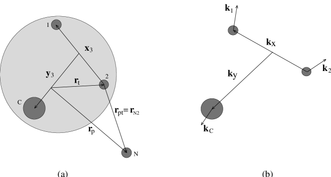
FIG. 1.: Spatial coordinates (a) in nucleon-nucleus scattering, and particle momenta (b) in the two-neutron halo system.

$$\mathchoice{{\hbox{\boldmath$\displaystyle k$}}}{{\hbox{\boldmath$\textstyle k$}}}{{\hbox{\boldmath$\scriptstyle k$}}}{{\hbox{\boldmath$\scriptscriptstyle k$}}}_{x} = \mu_{x}\Bigl{(}{\mathchoice{{\hbox{\boldmath$\displaystyle k$}}}{{\hbox{\boldmath$\textstyle k$}}}{{\hbox{\boldmath$\scriptstyle k$}}}{{\hbox{\boldmath$\scriptscriptstyle k$}}}_{1}\over m_{1}}-{\mathchoice{{\hbox{\boldmath$\displaystyle k$}}}{{\hbox{\boldmath$\textstyle k$}}}{{\hbox{\boldmath$\scriptstyle k$}}}{{\hbox{\boldmath$\scriptscriptstyle k$}}}_{2}\over m_{2}}\Bigr{)},\ \mu_{x}={m_{1}m_{2}\over m_{1}+m_{2}},$$ (3)

$$\mathchoice{{\hbox{\boldmath$\displaystyle k$}}}{{\hbox{\boldmath$\textstyle k$}}}{{\hbox{\boldmath$\scriptstyle k$}}}{{\hbox{\boldmath$\scriptscriptstyle k$}}}_{y} = \mu_{y}\Bigl{(}{\mathchoice{{\hbox{\boldmath$\displaystyle k$}}}{{\hbox{\boldmath$\textstyle k$}}}{{\hbox{\boldmath$\scriptstyle k$}}}{{\hbox{\boldmath$\scriptscriptstyle k$}}}_{C}\over m_{C}}-{\mathchoice{{\hbox{\boldmath$\displaystyle k$}}}{{\hbox{\boldmath$\textstyle k$}}}{{\hbox{\boldmath$\scriptstyle k$}}}{{\hbox{\boldmath$\scriptscriptstyle k$}}}_{1}+\mathchoice{{\hbox{\boldmath$\displaystyle k$}}}{{\hbox{\boldmath$\textstyle k$}}}{{\hbox{\boldmath$\scriptstyle k$}}}{{\hbox{\boldmath$\scriptscriptstyle k$}}}_{2}\over m_{1}+m_{2}}\Bigr{)},\ \mu_{y}={(m_{1}+m_{2})m_{C}\over m_{1}+m_{2}+m_{C}},$$ (4)

$$K = \mathchoice{{\hbox{\boldmath$\displaystyle k$}}}{{\hbox{\boldmath$\textstyle k$}}}{{\hbox{\boldmath$\scriptstyle k$}}}{{\hbox{\boldmath$\scriptscriptstyle k$}}}_{1}+\mathchoice{{\hbox{\boldmath$\displaystyle k$}}}{{\hbox{\boldmath$\textstyle k$}}}{{\hbox{\boldmath$\scriptstyle k$}}}{{\hbox{\boldmath$\scriptscriptstyle k$}}}_{2}+\mathchoice{{\hbox{\boldmath$\displaystyle k$}}}{{\hbox{\boldmath$\textstyle k$}}}{{\hbox{\boldmath$\scriptstyle k$}}}{{\hbox{\boldmath$\scriptscriptstyle k$}}}_{C}=-\mathchoice{{\hbox{\boldmath$\displaystyle k$}}}{{\hbox{\boldmath$\textstyle k$}}}{{\hbox{\boldmath$\scriptstyle k$}}}{{\hbox{\boldmath$\scriptscriptstyle k$}}}_{N}^{\prime}=-\mathchoice{{\hbox{\boldmath$\displaystyle k$}}}{{\hbox{\boldmath$\textstyle k$}}}{{\hbox{\boldmath$\scriptstyle k$}}}{{\hbox{\boldmath$\scriptscriptstyle k$}}}_{f}.$$ (5)

In the CM frame $E_{f}$ = $\varepsilon_{f}+E_{\kappa}+Q$, where $\varepsilon_{f}$ = ${\displaystyle{\hbar^{2}k_{f}^{2}\over 2\mu_{f}}}$, and $\mu_{f}$ = ${\displaystyle{m_{N}^{\prime}M_{A}\over m_{N}^{\prime}+M_{A}}}$ is the reduced mass for the exit channel, while $E_{\kappa}$ = $\varepsilon_{x}+\varepsilon_{y}$ = ${\displaystyle{\hbar^{2}k_{x}^{2}\over 2\mu_{x}}+{\hbar^{2}k_{y}^{2}\over 2\mu_{y}}}$ is the excitation energy measured from the breakup threshold. Taking into account conservation of energy and momenta, the exclusive cross section (when energies and momenta of all particles are observed) is an average over initial and a sum over final spin orientation, and can be written as

$${d^{5}\sigma\over d\Omega_{x}d\Omega_{y}d\Omega_{f}d\varepsilon_{y}dE_{\kappa}}=(2\pi)^{4}{\mu_{i}\mu_{f}\over\hbar^{4}}{k_{f}\over k_{i}}2({\mu_{x}\mu_{y}\over\hbar^{4}})^{3\over 2}\sqrt{\varepsilon_{y}(E_{\kappa}-\varepsilon_{y})}{1\over 2(2J_{i}+1)}\sum\mid\mbox{$T$}_{fi}\mid^{2}.$$ (6)

The factor $\sqrt{\varepsilon_{y}(E_{\kappa}-\varepsilon_{y})}$ describes the distribution of energy between different modes of particle motion, and reflects the phase-space accessible for breakup. The matrix element $T_{fi}$ includes all the interaction dynamics, and is given in the Distorted Wave (DW) framework by

$$\mbox{$T$}_{fi}=<\mbox{$\chi$}_{f,M_{b}}^{(-)}(\mathchoice{{\hbox{\boldmath$\displaystyle k$}}}{{\hbox{\boldmath$\textstyle k$}}}{{\hbox{\boldmath$\scriptstyle k$}}}{{\hbox{\boldmath$\scriptscriptstyle k$}}}_{f}),\mbox{$\Psi$}^{(-)}_{m_{1},m_{2},m_{C}}(\mathchoice{{\hbox{\boldmath$\displaystyle k$}}}{{\hbox{\boldmath$\textstyle k$}}}{{\hbox{\boldmath$\scriptstyle k$}}}{{\hbox{\boldmath$\scriptscriptstyle k$}}}_{x},\mathchoice{{\hbox{\boldmath$\displaystyle k$}}}{{\hbox{\boldmath$\textstyle k$}}}{{\hbox{\boldmath$\scriptstyle k$}}}{{\hbox{\boldmath$\scriptscriptstyle k$}}}_{y})\mid\sum_{t}V_{pt}\mid\mbox{$\Psi$}_{J_{i}M_{i}},\mbox{$\chi$}_{i,M_{a}}^{(+)}(\mathchoice{{\hbox{\boldmath$\displaystyle k$}}}{{\hbox{\boldmath$\textstyle k$}}}{{\hbox{\boldmath$\scriptstyle k$}}}{{\hbox{\boldmath$\scriptscriptstyle k$}}}_{i})>,$$ (7)

where $\mbox{$\chi$}_{i,f}^{(\pm)}$ are distorted waves describing relative motion of colliding nuclei, $\mbox{$\Psi$}_{J_{i}M_{i}}$ and $\mbox{$\Psi$}^{(-)}_{m_{1},m_{2},m_{C}}(\mathchoice{{\hbox{\boldmath$\displaystyle k$}}}{{\hbox{\boldmath$\textstyle k$}}}{{\hbox{\boldmath$\scriptstyle k$}}}{{\hbox{\boldmath$\scriptscriptstyle k$}}}_{x},\mathchoice{{\hbox{\boldmath$\displaystyle k$}}}{{\hbox{\boldmath$\textstyle k$}}}{{\hbox{\boldmath$\scriptstyle k$}}}{{\hbox{\boldmath$\scriptscriptstyle k$}}}_{y})$ are the initial bound and final continuum nuclear states, respectively. Spin projections $M_{a}$, $M_{i}$, $M_{b}$, $m_{1}$, $m_{2}$ and $m_{C}$, together with relative momenta $\mathchoice{{\hbox{\boldmath$\displaystyle k$}}}{{\hbox{\boldmath$\textstyle k$}}}{{\hbox{\boldmath$\scriptstyle k$}}}{{\hbox{\boldmath$\scriptscriptstyle k$}}}_{i,f}$ and $\mathchoice{{\hbox{\boldmath$\displaystyle k$}}}{{\hbox{\boldmath$\textstyle k$}}}{{\hbox{\boldmath$\scriptstyle k$}}}{{\hbox{\boldmath$\scriptscriptstyle k$}}}_{x,y}$ characterize the asymptotic state of all particles taking part in the reaction. Continuum wave functions are a matrix in spin space, and contain the probability for spin-flip in the course of scattering. Since we are interested in studying the ⁶He nucleus where the core is an $\alpha$-particle with spin zero, for simplification of notation we omit everywhere below mentioning of the core spin projection $m_{C}$.

In eq. (7) $V_{pt}$ is a local, effective nucleon-nucleon interaction between projectile and target nucleons $p$ and $t$, expressed in terms of central, spin-orbit and tensor components,

$$V(\mathchoice{{\hbox{\boldmath$\displaystyle r$}}}{{\hbox{\boldmath$\textstyle r$}}}{{\hbox{\boldmath$\scriptstyle r$}}}{{\hbox{\boldmath$\scriptscriptstyle r$}}}_{pt},\mathchoice{{\hbox{\boldmath$\displaystyle p$}}}{{\hbox{\boldmath$\textstyle p$}}}{{\hbox{\boldmath$\scriptstyle p$}}}{{\hbox{\boldmath$\scriptscriptstyle p$}}}_{pt})=\sum_{T}{\left\{\sum_{S}t_{ST}^{C}(r_{pt})\sigma_{p}^{S}\cdot\sigma_{t}^{S}+t_{LS}^{T}(r_{pt})\mathchoice{{\hbox{\boldmath$\displaystyle L$}}}{{\hbox{\boldmath$\textstyle L$}}}{{\hbox{\boldmath$\scriptstyle L$}}}{{\hbox{\boldmath$\scriptscriptstyle L$}}}\cdot\mathchoice{{\hbox{\boldmath$\displaystyle S$}}}{{\hbox{\boldmath$\textstyle S$}}}{{\hbox{\boldmath$\scriptstyle S$}}}{{\hbox{\boldmath$\scriptscriptstyle S$}}}+t_{T}^{T}(r_{pt})S_{pt}(\mathchoice{{\hbox{\boldmath$\displaystyle\hat{r}$}}}{{\hbox{\boldmath$\textstyle\hat{r}$}}}{{\hbox{\boldmath$\scriptstyle\hat{r}$}}}{{\hbox{\boldmath$\scriptscriptstyle\hat{r}$}}}_{pt})\right\}}\tau_{p}^{T}\cdot\tau_{t}^{T}$$ (8)

where $\mathchoice{{\hbox{\boldmath$\displaystyle r$}}}{{\hbox{\boldmath$\textstyle r$}}}{{\hbox{\boldmath$\scriptstyle r$}}}{{\hbox{\boldmath$\scriptscriptstyle r$}}}_{pt}=\mathchoice{{\hbox{\boldmath$\displaystyle r$}}}{{\hbox{\boldmath$\textstyle r$}}}{{\hbox{\boldmath$\scriptstyle r$}}}{{\hbox{\boldmath$\scriptscriptstyle r$}}}_{p}-\mathchoice{{\hbox{\boldmath$\displaystyle r$}}}{{\hbox{\boldmath$\textstyle r$}}}{{\hbox{\boldmath$\scriptstyle r$}}}{{\hbox{\boldmath$\scriptscriptstyle r$}}}_{t}$ and $\mathchoice{{\hbox{\boldmath$\displaystyle p$}}}{{\hbox{\boldmath$\textstyle p$}}}{{\hbox{\boldmath$\scriptstyle p$}}}{{\hbox{\boldmath$\scriptscriptstyle p$}}}_{pt}={1\over 2}(\mathchoice{{\hbox{\boldmath$\displaystyle p$}}}{{\hbox{\boldmath$\textstyle p$}}}{{\hbox{\boldmath$\scriptstyle p$}}}{{\hbox{\boldmath$\scriptscriptstyle p$}}}_{p}-\mathchoice{{\hbox{\boldmath$\displaystyle p$}}}{{\hbox{\boldmath$\textstyle p$}}}{{\hbox{\boldmath$\scriptstyle p$}}}{{\hbox{\boldmath$\scriptscriptstyle p$}}}_{t})$ are relative distance and momentum (wave number) between two nucleons, $\mathchoice{{\hbox{\boldmath$\displaystyle S$}}}{{\hbox{\boldmath$\textstyle S$}}}{{\hbox{\boldmath$\scriptstyle S$}}}{{\hbox{\boldmath$\scriptscriptstyle S$}}}={1\over 2}(\mathchoice{{\hbox{\boldmath$\displaystyle\sigma$}}}{{\hbox{\boldmath$\textstyle\sigma$}}}{{\hbox{\boldmath$\scriptstyle\sigma$}}}{{\hbox{\boldmath$\scriptscriptstyle\sigma$}}}_{p}+\mathchoice{{\hbox{\boldmath$\displaystyle\sigma$}}}{{\hbox{\boldmath$\textstyle\sigma$}}}{{\hbox{\boldmath$\scriptstyle\sigma$}}}{{\hbox{\boldmath$\scriptscriptstyle\sigma$}}}_{t})$ and $\mathchoice{{\hbox{\boldmath$\displaystyle L$}}}{{\hbox{\boldmath$\textstyle L$}}}{{\hbox{\boldmath$\scriptstyle L$}}}{{\hbox{\boldmath$\scriptscriptstyle L$}}}=\mathchoice{{\hbox{\boldmath$\displaystyle r$}}}{{\hbox{\boldmath$\textstyle r$}}}{{\hbox{\boldmath$\scriptstyle r$}}}{{\hbox{\boldmath$\scriptscriptstyle r$}}}_{pt}\times\mathchoice{{\hbox{\boldmath$\displaystyle p$}}}{{\hbox{\boldmath$\textstyle p$}}}{{\hbox{\boldmath$\scriptstyle p$}}}{{\hbox{\boldmath$\scriptscriptstyle p$}}}_{pt}$ are operators of total spin and orbital angular momentum of the two nucleons, $\mathchoice{{\hbox{\boldmath$\displaystyle p$}}}{{\hbox{\boldmath$\textstyle p$}}}{{\hbox{\boldmath$\scriptstyle p$}}}{{\hbox{\boldmath$\scriptscriptstyle p$}}}_{i}=-i\mathchoice{{\hbox{\boldmath$\displaystyle\nabla_{i}$}}}{{\hbox{\boldmath$\textstyle\nabla_{i}$}}}{{\hbox{\boldmath$\scriptstyle\nabla_{i}$}}}{{\hbox{\boldmath$\scriptscriptstyle\nabla_{i}$}}}$, $\sigma_{i}^{S}=1$, $\mathchoice{{\hbox{\boldmath$\displaystyle\sigma$}}}{{\hbox{\boldmath$\textstyle\sigma$}}}{{\hbox{\boldmath$\scriptstyle\sigma$}}}{{\hbox{\boldmath$\scriptscriptstyle\sigma$}}}_{i}$ for $S$=0, 1 respectively. $S_{pt}(\mathchoice{{\hbox{\boldmath$\displaystyle\hat{r}$}}}{{\hbox{\boldmath$\textstyle\hat{r}$}}}{{\hbox{\boldmath$\scriptstyle\hat{r}$}}}{{\hbox{\boldmath$\scriptscriptstyle\hat{r}$}}}_{pt})$ is the tensor operator

$$S_{pt}(\mathchoice{{\hbox{\boldmath$\displaystyle\hat{r}$}}}{{\hbox{\boldmath$\textstyle\hat{r}$}}}{{\hbox{\boldmath$\scriptstyle\hat{r}$}}}{{\hbox{\boldmath$\scriptscriptstyle\hat{r}$}}}_{pt}) = {3(\mathchoice{{\hbox{\boldmath$\displaystyle\sigma$}}}{{\hbox{\boldmath$\textstyle\sigma$}}}{{\hbox{\boldmath$\scriptstyle\sigma$}}}{{\hbox{\boldmath$\scriptscriptstyle\sigma$}}}_{p}\cdot\mathchoice{{\hbox{\boldmath$\displaystyle r$}}}{{\hbox{\boldmath$\textstyle r$}}}{{\hbox{\boldmath$\scriptstyle r$}}}{{\hbox{\boldmath$\scriptscriptstyle r$}}}_{pt})(\mathchoice{{\hbox{\boldmath$\displaystyle\sigma$}}}{{\hbox{\boldmath$\textstyle\sigma$}}}{{\hbox{\boldmath$\scriptstyle\sigma$}}}{{\hbox{\boldmath$\scriptscriptstyle\sigma$}}}_{t}\cdot\mathchoice{{\hbox{\boldmath$\displaystyle r$}}}{{\hbox{\boldmath$\textstyle r$}}}{{\hbox{\boldmath$\scriptstyle r$}}}{{\hbox{\boldmath$\scriptscriptstyle r$}}}_{pt})\over r_{pt}^{2}}-(\mathchoice{{\hbox{\boldmath$\displaystyle\sigma$}}}{{\hbox{\boldmath$\textstyle\sigma$}}}{{\hbox{\boldmath$\scriptstyle\sigma$}}}{{\hbox{\boldmath$\scriptscriptstyle\sigma$}}}_{p}\cdot\mathchoice{{\hbox{\boldmath$\displaystyle\sigma$}}}{{\hbox{\boldmath$\textstyle\sigma$}}}{{\hbox{\boldmath$\scriptstyle\sigma$}}}{{\hbox{\boldmath$\scriptscriptstyle\sigma$}}}_{t}).$$ (9)

Using the method of hyperspherical harmonics, the nuclear wave function above the breakup threshold can be written as follows (for details see Appendix A):

$$\mbox{$\Psi$}_{m_{1},m_{2}}^{(+)} = \sum_{\gamma,J_{f},M_{f},M_{L_{f}}}<s_{1}m_{1}\ s_{2}m_{2}\mid S_{f}M_{S_{f}}><L_{f}M_{L_{f}}S_{f}M_{S_{f}}\mid J_{f}M_{f}>$$ (10)

$$\times {\cal Y}^{l_{x}l_{y}\ \mbox{$*$}}_{K_{f}L_{f}M_{L_{f}}}(\Omega_{5}^{\kappa})\ \mbox{$\Psi$}_{\gamma,J_{f},M_{f}}(\mathchoice{{\hbox{\boldmath$\displaystyle x$}}}{{\hbox{\boldmath$\textstyle x$}}}{{\hbox{\boldmath$\scriptstyle x$}}}{{\hbox{\boldmath$\scriptscriptstyle x$}}},\mathchoice{{\hbox{\boldmath$\displaystyle y$}}}{{\hbox{\boldmath$\textstyle y$}}}{{\hbox{\boldmath$\scriptstyle y$}}}{{\hbox{\boldmath$\scriptscriptstyle y$}}},\kappa)$$ (11)

where $\gamma$ is an abbreviation for a set of quantum numbers $\gamma=\{K_{f},L_{f},S_{f},l_{x},l_{y}\}$, which characterizes the relative motion of the three particles flying apart. The continuum wave function $\mbox{$\Psi$}_{\gamma,J_{f},M_{f}}(\mathchoice{{\hbox{\boldmath$\displaystyle x$}}}{{\hbox{\boldmath$\textstyle x$}}}{{\hbox{\boldmath$\scriptstyle x$}}}{{\hbox{\boldmath$\scriptscriptstyle x$}}},\mathchoice{{\hbox{\boldmath$\displaystyle y$}}}{{\hbox{\boldmath$\textstyle y$}}}{{\hbox{\boldmath$\scriptstyle y$}}}{{\hbox{\boldmath$\scriptscriptstyle y$}}},\kappa)$ depends on the quantum numbers $\gamma$, Jacobian space coordinates $(\mathchoice{{\hbox{\boldmath$\displaystyle x$}}}{{\hbox{\boldmath$\textstyle x$}}}{{\hbox{\boldmath$\scriptstyle x$}}}{{\hbox{\boldmath$\scriptscriptstyle x$}}},\mathchoice{{\hbox{\boldmath$\displaystyle y$}}}{{\hbox{\boldmath$\textstyle y$}}}{{\hbox{\boldmath$\scriptstyle y$}}}{{\hbox{\boldmath$\scriptscriptstyle y$}}})$, nuclear excitation energy $E_{\kappa}$ (expressed by the hypermomentum $\kappa$), and the total angular momentum $J_{f}$ and its projections $M_{f}$,

$$\mbox{$\Psi$}_{\gamma,J_{f},M_{f}}(\mathchoice{{\hbox{\boldmath$\displaystyle x$}}}{{\hbox{\boldmath$\textstyle x$}}}{{\hbox{\boldmath$\scriptstyle x$}}}{{\hbox{\boldmath$\scriptscriptstyle x$}}},\mathchoice{{\hbox{\boldmath$\displaystyle y$}}}{{\hbox{\boldmath$\textstyle y$}}}{{\hbox{\boldmath$\scriptstyle y$}}}{{\hbox{\boldmath$\scriptscriptstyle y$}}},\kappa)={\displaystyle{1\over(\kappa\rho)^{5/2}}\ \sum_{\gamma^{\prime},M^{\prime}_{L}}\mbox{$\chi$}_{K^{\prime}l^{\prime}_{x}l^{\prime}_{y},K_{f}l_{x}l_{y}}^{L^{\prime}S^{\prime},L_{f}S_{f}}(\kappa\rho)\ \Upsilon^{l^{\prime}_{x}l^{\prime}_{y}}_{J_{f}K^{\prime}L^{\prime}S^{\prime}M_{f}}(\Omega_{5})}$$ (12)

The transition amplitude $T_{fi}$ can be further decomposed according to eq. (10),

$$\mbox{$T$}_{fi}=\!\sum_{\gamma,M_{L_{f}},M_{S_{f}}}\!<s_{1}m_{1}s_{2}m_{2}\mid S_{f}M_{S_{f}}>\ <L_{f}M_{L_{f}}S_{f}M_{S_{f}}\mid J_{f}M_{f}>\ {\cal Y}^{l_{x}l_{y}\ \mbox{$*$}}_{K_{f}L_{f}M_{L_{f}}}(\Omega_{5}^{\kappa})\ \mbox{$T$}_{\gamma}(\mathchoice{{\hbox{\boldmath$\displaystyle k$}}}{{\hbox{\boldmath$\textstyle k$}}}{{\hbox{\boldmath$\scriptstyle k$}}}{{\hbox{\boldmath$\scriptscriptstyle k$}}}_{x},\mathchoice{{\hbox{\boldmath$\displaystyle k$}}}{{\hbox{\boldmath$\textstyle k$}}}{{\hbox{\boldmath$\scriptstyle k$}}}{{\hbox{\boldmath$\scriptscriptstyle k$}}}_{y},\kappa)$$ (13)

where $T_{\gamma}(\mathchoice{{\hbox{\boldmath$\displaystyle k$}}}{{\hbox{\boldmath$\textstyle k$}}}{{\hbox{\boldmath$\scriptstyle k$}}}{{\hbox{\boldmath$\scriptscriptstyle k$}}}_{x},\mathchoice{{\hbox{\boldmath$\displaystyle k$}}}{{\hbox{\boldmath$\textstyle k$}}}{{\hbox{\boldmath$\scriptstyle k$}}}{{\hbox{\boldmath$\scriptscriptstyle k$}}}_{y},\kappa)$ formally now has the same structure as any two-body amplitude for excitation of a nuclear state with total momentum $J_{f},M_{f}$, excitation energy $E_{\kappa}$, and a fixed state of relative motion of breakup fragments defined by the quantum numbers $\gamma$:

$$\mbox{$T$}_{\gamma}(\mathchoice{{\hbox{\boldmath$\displaystyle k$}}}{{\hbox{\boldmath$\textstyle k$}}}{{\hbox{\boldmath$\scriptstyle k$}}}{{\hbox{\boldmath$\scriptscriptstyle k$}}}_{x},\mathchoice{{\hbox{\boldmath$\displaystyle k$}}}{{\hbox{\boldmath$\textstyle k$}}}{{\hbox{\boldmath$\scriptstyle k$}}}{{\hbox{\boldmath$\scriptscriptstyle k$}}}_{y},\kappa) = <\mbox{$\chi$}_{f,M_{b}}^{(-)}(\mathchoice{{\hbox{\boldmath$\displaystyle k$}}}{{\hbox{\boldmath$\textstyle k$}}}{{\hbox{\boldmath$\scriptstyle k$}}}{{\hbox{\boldmath$\scriptscriptstyle k$}}}_{f}),\mbox{$\Psi$}_{\gamma,J_{f},M_{f}}(\kappa)\mid\sum_{t}V_{pt}\mid\mbox{$\Psi$}_{J_{i}M_{i}},\mbox{$\chi$}_{i,M_{a}}^{(+)}(\mathchoice{{\hbox{\boldmath$\displaystyle k$}}}{{\hbox{\boldmath$\textstyle k$}}}{{\hbox{\boldmath$\scriptstyle k$}}}{{\hbox{\boldmath$\scriptscriptstyle k$}}}_{i})>$$ (14)

$$= \sum_{jm}\ <J_{i}M_{i}\ jm\mid J_{f}M_{f}>\ \mbox{$T$}_{\gamma,j}^{M_{a},M_{b},m}(\mathchoice{{\hbox{\boldmath$\displaystyle k$}}}{{\hbox{\boldmath$\textstyle k$}}}{{\hbox{\boldmath$\scriptstyle k$}}}{{\hbox{\boldmath$\scriptscriptstyle k$}}}_{x},\mathchoice{{\hbox{\boldmath$\displaystyle k$}}}{{\hbox{\boldmath$\textstyle k$}}}{{\hbox{\boldmath$\scriptstyle k$}}}{{\hbox{\boldmath$\scriptscriptstyle k$}}}_{y},\kappa)$$ (15)

To calculate the reaction amplitude we use the partial wave decomposition for the distorted waves $\mbox{$\chi$}^{(+)}_{i,M_{a}}(\mathchoice{{\hbox{\boldmath$\displaystyle k$}}}{{\hbox{\boldmath$\textstyle k$}}}{{\hbox{\boldmath$\scriptstyle k$}}}{{\hbox{\boldmath$\scriptscriptstyle k$}}}_{i})$, describing the relative motion of the projectile nucleon and the center of mass of the target nucleus:

$$\mbox{$\chi$}^{(+)}_{i,M_{a}}(\mathchoice{{\hbox{\boldmath$\displaystyle k$}}}{{\hbox{\boldmath$\textstyle k$}}}{{\hbox{\boldmath$\scriptstyle k$}}}{{\hbox{\boldmath$\scriptscriptstyle k$}}}_{i}) = \sum_{M_{a}^{\prime}}\mbox{$\chi$}^{(+)}_{i,M_{a}^{\prime}M_{a}}(\mathchoice{{\hbox{\boldmath$\displaystyle k$}}}{{\hbox{\boldmath$\textstyle k$}}}{{\hbox{\boldmath$\scriptstyle k$}}}{{\hbox{\boldmath$\scriptscriptstyle k$}}}_{i},\mathchoice{{\hbox{\boldmath$\displaystyle r$}}}{{\hbox{\boldmath$\textstyle r$}}}{{\hbox{\boldmath$\scriptstyle r$}}}{{\hbox{\boldmath$\scriptscriptstyle r$}}}_{p})|S_{a}M_{a}^{\prime}\rangle$$ (16)

$$= {4\pi\over k_{i}r_{p}}\sum_{l_{a}j_{a}}\ <l_{a}m_{l_{a}}S_{a}M_{a}|j_{a}m_{a}>\ i^{l_{a}}\ Y_{l_{a}m_{l_{a}}}^{\mbox{$*$}}(\mathchoice{{\hbox{\boldmath$\displaystyle\hat{k}$}}}{{\hbox{\boldmath$\textstyle\hat{k}$}}}{{\hbox{\boldmath$\scriptstyle\hat{k}$}}}{{\hbox{\boldmath$\scriptscriptstyle\hat{k}$}}}_{i})\ \mbox{$\chi$}_{l_{a}j_{a}}(k_{i},r_{p})\ |j_{a}m_{a}\rangle$$ (17)

where $|j_{a}m_{a}\rangle=\sum\ <l_{a}m_{l_{a}}^{\prime}S_{a}M^{\prime}_{a}|j_{a}m_{a}>\ Y_{l_{a}m_{l_{a}}^{\prime}}(\mathchoice{{\hbox{\boldmath$\displaystyle\hat{r}$}}}{{\hbox{\boldmath$\textstyle\hat{r}$}}}{{\hbox{\boldmath$\scriptstyle\hat{r}$}}}{{\hbox{\boldmath$\scriptscriptstyle\hat{r}$}}}_{p})\ |S_{a}M^{\prime}_{a}\rangle$, and $|S_{a}M^{\prime}_{a}\rangle$ is the projectile spin function. Nuclear formfactors can be defined as follows

$$<j_{b}m_{b},J_{f}M_{f}\mid\sum_{t}V_{pt}\mid J_{i}M_{i},j_{a}m_{a}>\ =\sum_{lsj}<J_{i}M_{i}jm\mid J_{f}M_{f}>$$ (19)

$$\times\imath^{-l}\ {(-1)^{l+s-j+m}\over\hat{s}}\ <j_{b}m_{b}\mid[Y_{l}(\mathchoice{{\hbox{\boldmath$\displaystyle\hat{r}$}}}{{\hbox{\boldmath$\textstyle\hat{r}$}}}{{\hbox{\boldmath$\scriptstyle\hat{r}$}}}{{\hbox{\boldmath$\scriptscriptstyle\hat{r}$}}}_{p})\otimes\sigma^{s}_{p}]_{jm}\mid j_{a}m_{a}>F_{j_{b}j_{a}}^{lsj}(\kappa,r_{p},{\partial\over\partial r_{p}})$$

where $\hat{s}=\sqrt{2s+1}$. In the case of nuclear excitations of normal and unnatural parity the explicit formulas for radial formfactor $F_{j_{b}j_{a}}^{lsj}$ are given in [31] and Appendix B. Taking into account these definitions the reaction amplitude $T_{\gamma,j}^{M_{a},M_{b},m}(\mathchoice{{\hbox{\boldmath$\displaystyle k$}}}{{\hbox{\boldmath$\textstyle k$}}}{{\hbox{\boldmath$\scriptstyle k$}}}{{\hbox{\boldmath$\scriptscriptstyle k$}}}_{x},\mathchoice{{\hbox{\boldmath$\displaystyle k$}}}{{\hbox{\boldmath$\textstyle k$}}}{{\hbox{\boldmath$\scriptstyle k$}}}{{\hbox{\boldmath$\scriptscriptstyle k$}}}_{y},\kappa)$ can be written in usual form

$$\mbox{$T$}_{\gamma,j}^{M_{a},M_{b},m}(\mathchoice{{\hbox{\boldmath$\displaystyle k$}}}{{\hbox{\boldmath$\textstyle k$}}}{{\hbox{\boldmath$\scriptstyle k$}}}{{\hbox{\boldmath$\scriptscriptstyle k$}}}_{x},\mathchoice{{\hbox{\boldmath$\displaystyle k$}}}{{\hbox{\boldmath$\textstyle k$}}}{{\hbox{\boldmath$\scriptstyle k$}}}{{\hbox{\boldmath$\scriptscriptstyle k$}}}_{y},\kappa)={(4\pi)^{2}\over k_{i}k_{f}}\sum_{l_{a}j_{a}l_{b}j_{b}ls}i^{l_{a}-l_{b}-l}\ Y_{l_{a}m_{l_{a}}}^{\mbox{$*$}}(\mathchoice{{\hbox{\boldmath$\displaystyle\hat{k}$}}}{{\hbox{\boldmath$\textstyle\hat{k}$}}}{{\hbox{\boldmath$\scriptstyle\hat{k}$}}}{{\hbox{\boldmath$\scriptscriptstyle\hat{k}$}}}_{i})\ Y_{l_{b}m_{l_{b}}}(\mathchoice{{\hbox{\boldmath$\displaystyle\hat{k}$}}}{{\hbox{\boldmath$\textstyle\hat{k}$}}}{{\hbox{\boldmath$\scriptstyle\hat{k}$}}}{{\hbox{\boldmath$\scriptscriptstyle\hat{k}$}}}_{f})\ \mbox{$I$}_{l_{a}j_{a},l_{b}j_{b}}^{lsj}\ {\hat{j}\hat{j}_{b}\sqrt{2}\hat{l}_{b}\hat{l}\over\sqrt{4\pi}}$$ (20)

$$\times <l_{a}m_{l_{a}}S_{a}M_{a}|j_{a}m_{a}>\ <l_{b}m_{l_{b}}S_{b}M_{b}|j_{b}m_{b}>\ <j_{b}m_{b}jm|j_{a}m_{a}>\ <l_{b}0l0|l_{a}0>\ {\left\{\begin{array}[]{ccc}l_{b}&S_{b}&j_{b}\\ l&s&j\\ l_{a}&S_{a}&j_{a}\end{array}\right\}}$$ (24)

where the radial integrals $I_{l_{a}j_{a},l_{b}j_{b}}^{lsj}$ are defined as follows

$$\mbox{$I$}_{l_{a}j_{a},l_{b}j_{b}}^{lsj}=\int_{0}^{\infty}dr_{p}\ r_{p}^{2}\ {1\over r_{p}}\ \mbox{$\chi$}_{l_{b}j_{b}}(k_{f},r_{p})\ F^{lsj}_{j_{a}j_{b}}(\kappa,r_{p},{\partial\over\partial r_{p}})\ {1\over r_{p}}\ \mbox{$\chi$}_{l_{a}j_{a}}(k_{i},r_{p})$$ (25)

It is useful to compare the expression (13) for the breakup amplitude $T_{fi}$ with the amplitude for a usual two-body reaction which has the same structure as amplitude (15). In the 3-body case, the amplitude $T_{fi}$ has additional degrees of freedom which are manifested as dependence on angles $\Omega_{5}^{\kappa}=\{\alpha,\mathchoice{{\hbox{\boldmath$\displaystyle\hat{k}$}}}{{\hbox{\boldmath$\textstyle\hat{k}$}}}{{\hbox{\boldmath$\scriptstyle\hat{k}$}}}{{\hbox{\boldmath$\scriptscriptstyle\hat{k}$}}}_{x},\mathchoice{{\hbox{\boldmath$\displaystyle\hat{k}$}}}{{\hbox{\boldmath$\textstyle\hat{k}$}}}{{\hbox{\boldmath$\scriptstyle\hat{k}$}}}{{\hbox{\boldmath$\scriptscriptstyle\hat{k}$}}}_{y}\}$, where $\sin^{2}\alpha={\displaystyle{\varepsilon_{x}\over E_{\kappa}}}$. In contrast to a traditional two-body approach, the exclusive cross section (proportional to $\mid T_{fi}\mid^{2}$) contains an incoherent sum over total spin $S_{f}$ but a coherent sum over total transferred $j$ and final $J_{f}$. Consequently, we expect that the exclusive cross section will be especially sensitive to the correlations in the nuclear structure.

The different exclusive cross sections and correlation distributions will be considered elsewhere, here we restrict ourselves to inclusive cross sections. To calculate the double-differential inclusive cross sections when experiments measure the energy and angle for one particle, we must integrate the fivefold exclusive cross section (6) over the unobserved coordinates of breakup particles (angles $\mathchoice{{\hbox{\boldmath$\displaystyle\hat{x}$}}}{{\hbox{\boldmath$\textstyle\hat{x}$}}}{{\hbox{\boldmath$\scriptstyle\hat{x}$}}}{{\hbox{\boldmath$\scriptscriptstyle\hat{x}$}}}=\Omega_{x}$, $\mathchoice{{\hbox{\boldmath$\displaystyle\hat{y}$}}}{{\hbox{\boldmath$\textstyle\hat{y}$}}}{{\hbox{\boldmath$\scriptstyle\hat{y}$}}}{{\hbox{\boldmath$\scriptscriptstyle\hat{y}$}}}=\Omega_{y}$), and over various distributions of relative energy $\varepsilon_{y}$ between fragments:

$${d^{2}\sigma\over d\Omega_{f}dE_{\kappa}}=\int_{0}^{E_{\kappa}}d\varepsilon_{y}\int d\Omega_{x}d\Omega_{y}{d^{5}\sigma\over d\Omega_{x}d\Omega_{y}d\Omega_{f}d\varepsilon_{y}dE_{\kappa}}$$ (26)

Using the following orthogonality properties of the hyperspherical harmonics,

$$\int_{0}^{E_{\kappa}}d\varepsilon_{y}\sqrt{\varepsilon_{y}(E_{\kappa}-\varepsilon_{y})}\int d\Omega_{x}d\Omega_{y}{\cal Y}_{K^{\prime}L^{\prime}M_{L}^{\prime}}^{l_{x}^{\prime}l_{y}^{\prime}\mbox{$*$}}(\Omega_{5}^{\kappa}){\cal Y}_{KLM_{L}}^{l_{x}l_{y}}(\Omega_{5}^{\kappa})$$ (27)

$$=\ 2E_{\kappa}^{2}\delta_{K^{\prime}K}\delta_{L^{\prime}L}\delta_{M_{L}^{\prime}M_{L}}\delta_{l_{x}^{\prime}l_{x}}\delta_{l_{y}^{\prime}l_{y}},$$ (28)

the inclusive cross section now becomes an incoherent sum over total transferred $j$ and final $J_{f}$ angular momenta, and different $\gamma$-components of the final target state are excited independently of each other. Thus

$${d^{2}\sigma\over d\Omega_{f}dE_{\kappa}} = (2\pi)^{4}{\mu_{i}\mu_{f}\over\hbar^{4}}{k_{f}\over k_{i}}\sum_{j,J_{f},\gamma}{(2J_{f}+1)\over(2J_{i}+1)(2j+1)}$$ (29)

$$\times {1\over 2}\sum_{mm_{a}m_{b}}\mid\mbox{$T$}_{\gamma,j}^{m_{a}m_{b}m}(\mathchoice{{\hbox{\boldmath$\displaystyle k$}}}{{\hbox{\boldmath$\textstyle k$}}}{{\hbox{\boldmath$\scriptstyle k$}}}{{\hbox{\boldmath$\scriptscriptstyle k$}}}_{f},\mathchoice{{\hbox{\boldmath$\displaystyle k$}}}{{\hbox{\boldmath$\textstyle k$}}}{{\hbox{\boldmath$\scriptstyle k$}}}{{\hbox{\boldmath$\scriptscriptstyle k$}}}_{i},\kappa)\mid^{2}4E_{\kappa}^{2}({\mu_{x}\mu_{y}\over\hbar^{4}})^{{3\over 2}}.$$ (30)

In this expression the factor $E_{\kappa}^{2}$, which originates from the 3-body phase volume, guarantees the correct cross section behavior at the breakup threshold. From (30) it also follows that, due to the averaging procedure, we lose information about correlations in relative motion of the breakup particles (which were defined by ${\cal Y}_{KLM_{L}}^{l_{x}l_{y}}(\Omega_{5}^{\kappa})$ hyperharmonics); remnants of the complex dynamics that governs the particles motion are kept only in different shapes and strengths with which various components of final states are distributed over excitation energies. One may hope that in the differential inclusive cross sections, due to specifics of reaction mechanisms, we can under certain conditions enhance the excitations of some of the components and thus still obtain valuable information about structures of halo nuclei.

The inclusive excitation cross section can be obtained by integrating over all ejectile angles $\Omega_{f}$:

$${d\sigma\over dE_{\kappa}}=\int d\Omega_{f}{d^{2}\sigma\over d\Omega_{f}dE_{\kappa}}.$$ (31)

This cross section describes the distribution of total strength of different excitation modes over energy spectra in quasielastic reactions.

V Results

With the model described above, we have calculated the excitation (eq. 31) and double-differential (eq. 30) inclusive spectra in the CM system for the charge-exchange reaction ⁶Li(n,p)⁶He and the inelastic scattering ⁶He(p,p^′)⁶He at $E_{N}$ = 50 MeV, with excitation of different $J_{f}^{\pi_{f}}=0^{\pm},1^{\pm},2^{\pm},3^{\pm}$ low-energy states of ⁶He. The corresponding cross sections are shown in Figs. 3-6. In the figures $E^{*}$ is the nuclear excitation energy measured from ⁶He ground state. For inelastic scattering the initial target state of ⁶He has $J_{i}$ = 0 and the total $j$ transferred has a unique value and coincides with $J_{f}$ of the final state. For charge-exchange on ⁶Li the situation is more complex: since $J_{i}$ = 1 for the ⁶Li ground state it is possible to excite final states of ⁶He with definite $J_{f}$ by different $j$ transfers. All values of $j$ allowed by angular momentum conservation ($\mathchoice{{\hbox{\boldmath$\displaystyle J$}}}{{\hbox{\boldmath$\textstyle J$}}}{{\hbox{\boldmath$\scriptstyle J$}}}{{\hbox{\boldmath$\scriptscriptstyle J$}}}_{i}-\mathchoice{{\hbox{\boldmath$\displaystyle J$}}}{{\hbox{\boldmath$\textstyle J$}}}{{\hbox{\boldmath$\scriptstyle J$}}}{{\hbox{\boldmath$\scriptscriptstyle J$}}}_{f}=\mathchoice{{\hbox{\boldmath$\displaystyle j$}}}{{\hbox{\boldmath$\textstyle j$}}}{{\hbox{\boldmath$\scriptstyle j$}}}{{\hbox{\boldmath$\scriptscriptstyle j$}}}$) were taken into account in our calculations. It follows from equation (30) that every $j$ gives an independent contribution to the inclusive cross sections.

Our main goal is to demonstrate, that even in the simplest inclusive experiments it is still possible to extract information about structures in the continuum by detailed examination of both excitation and differential cross-sections.

A Two test cases for the model

Two cases were used to check the model and consistency of our reaction continuum calculations. The sharp $2^{+}_{1}$ resonance at 1.8 MeV was used in the first. This resonance resembles a usual bound state and can be described with good accuracy by calculating it with a boundary condition under the barrier corresponding to a discrete state. We use this to calculate the differential cross section ${\displaystyle{d\sigma\over d\Omega}}$. Next we calculate the double-differential ${\displaystyle{d^{2}\sigma\over d\Omega dE^{*}}}$ cross sections for the $2^{+}_{1}$ resonance at different $E^{*}$ and after that integrate over $E^{*}$ across the resonance. In fact, calculating a resonance width and cross section at peak position, energy integration has been done analytically since the resonance has the Breit-Wigner form (we checked it). In both calculations we got the same results for ${\displaystyle{d\sigma\over d\Omega}}$.

The second way is to compare our calculation with known experimental data for excitation to the continuum. In work [34] the reaction ⁶Li(n,p)⁶He at neutron energy 118 MeV was measured. The proton energy resolution in the experiment was $\sim$ 2.3 MeV. This should be kept in mind when comparing with the reported differential cross sections for transitions from the $1^{+}$ ground state of ⁶Li to the $0^{+}$ ground state and $2^{+}_{1}$ resonance (1.8 MeV) of ⁶He. Fig. 2 shows the corresponding experimental data plotted together with our calculations using the Love and Franey $t$-matrix interaction [32] at 100 MeV and an optical potential [39] describing proton elastic scattering from ⁶Li at 144 MeV. A good description for the shape and absolute value of the differential cross section to ground state was obtained and also a reasonable agreement with the data on the $2^{+}$ resonance. The $2^{+}$ angular distribution has a characteristic form corresponding to a transition of mixed angular momenta. To demonstrate this we show in Fig. 2b the separate contributions from transitions with total transferred $j$ equal 1, 2 and 3 by dashed, dotted and dashed-dotted lines, respectively. The transition with $j$ = 1 includes transfer of relative orbital momentum $l$ = 0 and determines the cross section at small angles, the others with $j$ = 2 and 3 have $l$ = 2 and dominate at larger angles.

Thus the reliability of our approach was confirmed, arguing for our predictions for low-energy excitation spectra, for which the model was developed.

FIG. 2.: Angular distributions for ⁶Li(n,p)⁶He at 118 MeV. The dashed, dotted and dashed-dotted lines show the contributions from $j=1,2\mbox{ and }3$, respectively. The experimental data are from ref. [34].

B Inclusive excitation spectra

FIG. 3.: Multipole $J^{\pi_{f}}_{f}$ and spin decomposition (left and right sides) of inclusive proton energy spectra from ⁶Li(n,p)⁶He^∗ (top row) and ⁶He(p,p^′)⁶He^∗ (bottom row) reactions.

FIG. 4.: The electromagnetic and nuclear inelastic cross section for $1^{-}$ excitation.

1 Partial content

The inclusive excitation spectra (Fig. 3, thick solid line) for charge-exchange and inelastic scattering reveal two distinguished bumps in the low-energy total spectrum : The first, narrow at excitation energy $\sim$ 1.8 MeV and the second, broad at $\sim$ 4.5 MeV. To understand the nature of these structures, the left side of Fig. 3 shows the decomposition of the total spectra into contributions from excitations of different partial components $J_{f}^{\pi}$ of ⁶He. The $1^{-}$, $2^{+}$ and $0^{+}$ excitations are given by thin solid, dashed and dotted lines, respectively. The dot-dashed line shows the contribution from $1^{+}$ excitation for charge-exchange and $3^{-}$ for inelastic scattering. Contributions from other partial waves are less significant and not given in the figure.

The first narrow peak is the well-known $2^{+}_{1}$ resonance in ⁶He. The broad bump has a more complex structure. A mixture of different excitations is responsible for the total shape; a second $2^{+}$ resonance and concentration of low lying strength of $1^{-}$ and $0^{+}$ excitations dominate the spectrum. The double-hump shape of $2^{+}$ excitations is the most remarkable feature of the low-energy spectrum. The strength concentration of $1^{-}$ transitions at $E_{x}\sim$ 4 MeV is the other peculiarity. The behavior of other excitations, for example $3^{-}$, is different. It smoothly increases from threshold, and in the case of inelastic scattering gives a significant contribution at higher excitation energy.

The excitation spectra for both reactions have qualitatively the same gross structure, but the absolute cross sections are a few times larger for inelastic scattering than for charge-exchange.

Nuclear reactions in which halo nuclei take part serve, due to somewhat different dynamics, like filters and could lead to different multipole composition in observed excitation structures. In inelastic scattering the dipole mode dominates while in charge-exchange the $2^{+}$ resonance is about 50$\%$ larger.

The pronounced $1^{-}$ nuclear excitation has similarities with electromagnetic response for the soft dipole mode, prevalent in Coulomb breakup on heavy targets. Fig. 4 shows theoretical cross sections for Coulomb breakup (dotted line) of ⁶He on gold at 63 MeV/A and inelastic proton scattering (solid line) with $1^{-}$ excitations, arbitrarily normalized. A semiclassical description is used for the Coulomb dissociation process and our model for the electromagnetic dipole response in ⁶He [6]. Both processes show strength accumulation in the same energy region and hence, we should expect no matter which excitation mechanism dominates, a similar behaviour for excitation functions. In an elegant experiment on ⁶He breakup reaction at 63.2 MeV/nucleon on Al and Au targets [24] with registration of $\gamma-$rays in coincidence, similar behaviour of $\alpha-$particle distributions was found for both targets. For the light Al target, nuclear mechanism is believed to give the main contribution to the spectra while for Au the EM dominates. Our theoretical results explain qualitatively the observed similarity.

2 Spin structure

The composition of spectra, or relative role of excitations of various $J^{\pi_{f}}_{f}$, is as discussed above different for the two reactions. In charge-exchange a relatively larger number of states was excited with about equal intensity, while inelastic scattering is more selective. To better illustrate this point, the right side of Fig. 3 shows separately the contributions from excitations of ⁶He states with total spin $S_{f}$ = 0 (dashed line) and 1 (dotted line). For inelastic scattering the excitations with $S_{f}$ = 0 dominate the spectrum, while for charge-exchange both contributions become comparable. This is a reflection of specific reaction mechanisms. In inelastic scattering the S = 0, T = 0 component of effective interactions is the biggest one, while in charge-exchange only isovector components play a role and in the charge channel the effective forces with S = 0 and S = 1 are comparable in strength. The relative role of different components of effective forces depends on collision energy and so the ratio between excitations of the various structures will change accordingly.

C Double-differential inclusive cross sections

1 Fixed angle

Excitation functions, measured at a fixed angle, can serve as a filter for selecting partial waves with definite multipolarity and therefore make it possible to extract information on resonances in complex situations like that described above.

Fig. 5 shows spectra for charge-exchange at different exit proton angles. The total, $1^{-}$, $2^{+}$, $0^{+}$ and $1^{+}$ spectra are denoted by thick solid, thin solid, dashed, dotted and dashed-dotted lines, respectively. The double-hump shape appears at all angles, but the composition of the second bump depends on scattering angle or angular momenta transferred in the reaction. At 0^∘ the excitation of $0^{+}$, $1^{+}$ and $2^{+}$ dominates the spectrum. All are populated by strong transitions with relative orbital momentum $l$ = 0. With increasing angle the excitation of $1^{-}$ grows and at 10^∘ all these states are important. At 20^∘ the $1^{-}$ and $2^{+}$ are most pronounced. At 40^∘ the absolute cross section has been reduced to half value, and all energy spectra except $2^{+}$ have flat distributions. It is also interesting to note that for $1^{-}$ excitation the main contribution comes from the transition with $j=2$, $s=1$ and $l=1$. The dominance of spin-flip transition is due to the structure of initial and final states where components with $S_{i}=1$ and $S_{f}=0$ prevail.

FIG. 5.: Inclusive differential proton energy spectra from ⁶Li(n,p)⁶He^∗ for four values of the scattering angle $\theta_{cm}$. See the text for further details.

Fig.  6 shows the analogous spectra for inelastic scattering. All lines mean the same as in the previous figure, except that the dotted line denotes $3^{-}$ excitation for $\theta$ = 20^∘ and 40^∘. At 0^∘ the $0^{+}$ is excited very effectively in the region of the second bump. With increasing scattering angle $1^{-}$ becomes pronounced. It dominates the total spectra at 10^∘ and 20^∘. Contributions from $2^{+}$ and $1^{+}$ additionally increase the width of this bump. At 40^∘ the total cross section is again diminished, with $2^{+}$ and $1^{-}$ excitations being the largest. At higher excitation energy $3^{-}$ now gives a significant contribution to the total spectrum.

FIG. 6.: Inclusive differential proton energy spectra from ⁶He(p,p^′)⁶He^∗ for four values of the scattering angle $\theta_{cm}$. See the text for further details.

From the results represented in the figures, it follows that the second bump structure in the low-energy part of the spectra is a complex mixture of various excitations of the ⁶He nucleus. The way these excitations are revealed depends on the external fields (or reactions) applied to the system. This is a characteristic feature of continuum excitations without sharp resonances.

2 Fixed excitation energy

We discussed above the dependence of the differential cross sections on excitation energy for fixed scattering angle or momentum transfer. It is also interesting to compare the behavior of the cross sections at fixed excitation energy for different scattering angles. Fig. 7 shows angular distributions for the (n,p) reaction, for a few excitation energies that cover both sides of the second bump. The values of the transferred momenta $\textstyle q$=$\mathchoice{{\hbox{\boldmath$\displaystyle k$}}}{{\hbox{\boldmath$\textstyle k$}}}{{\hbox{\boldmath$\scriptstyle k$}}}{{\hbox{\boldmath$\scriptscriptstyle k$}}}_{i}-\mathchoice{{\hbox{\boldmath$\displaystyle k$}}}{{\hbox{\boldmath$\textstyle k$}}}{{\hbox{\boldmath$\scriptstyle k$}}}{{\hbox{\boldmath$\scriptscriptstyle k$}}}_{f}$ (in units of fm^-1) are shown on the top abscissa, corresponding to the scattering angles shown at the bottom abscissa. The thick solid line shows the total cross section. On the left side of the bump ($E^{*}$ = 3.5 MeV, Fig. 7a) the differential cross section has an asymmetric bell shape with maximum at about 15^∘. Going to higher excitation energy ($E^{*}$ = 4.1 MeV,

FIG. 7.: Proton energy spectra from the ⁶Li(n,p)⁶He^∗ versus scattering angle $\theta_{cm}$ for four excitation energies $E^{*}$.

Fig. 7b) through the bump maximum($E^{*}$ = 4.5 MeV, Fig. 7c) to the right side ($E^{*}$ = 5.2 MeV, Fig. 7d), the cross section shape changes smoothly and becomes gradually more flat with a plateau from 0^∘ to 20^∘ on the high energy side. This shape modification becomes transparent if we examine how the contributions from excitations of different $J^{\pi_{f}}_{f}$ change with energy. The thin solid, dotted, dashed and dash-dotted curves show the contributions of $0^{+}$, $1^{-}$, $1^{+}$ and $2^{+}$, respectively. We see that at small angles, the dominating states are all those ($0^{+}$, $1^{+}$ and $2^{+}$) which can be reached by transitions with zero relative orbital momentum. For a range of somewhat larger angles the contribution of $1^{-}$ is most significant. The $0^{+}$ and $1^{+}$ have smoothly falling angular distributions, $2^{+}$ is more flat due to the already mentioned mixing of transitions with different $j$. Hence, the interplay between $0^{+}$, $1^{+}$ and $2^{+}$ excitations, which together create a smooth background with highest cross section at small angles, and the $1^{-}$ peaking at 20^∘, define the total shape. The competition between them is responsible for the modification of this shape with excitation energy. As a result, we get a flat total distribution extending over a rather wide angular range on the high-energy slope of the second bump. These results are in qualitative agreement with experimental data on the ⁶Li(⁷Li,${}^{7}Be$)⁶He^∗ reaction [27, 28] if we scale angular distribution according to the transferred momentum $q$.

The corresponding data for inelastic scattering are shown in Fig. 8. The thick solid, thin solid, dashed and dotted lines again show total, $0^{+}$, $1^{-}$ and $2^{+}$ cross sections, respectively. For inelastic scattering, in contrast to charge-exchange, the total cross section remains bell-shaped at all excitation energies of the second bump. This is caused by the dipole excitation which dominates the spectra. The contribution from $0^{+}$ is also significant, especially at small scattering angles, counteracting the drop of the total cross section. The excitation of $2^{+}$ in (p,p^′) does not play the prominent role it does in charge-exchange. Together, $0^{+}$ and $2^{+}$, create a smooth background in angular distributions.

FIG. 8.: Proton energy spectra from ⁶He(p,p^′)⁶He^∗ versus scattering angle $\theta_{cm}$ for four excitation energies $E^{*}$.

These differences in the two reactions are due to two reasons: i) because of different structure of initial states we need different operators to excite the same final state in ⁶He and ii) in addition to isovector forces in charge-exchange the strong isoscalar NN interaction acts between target and projectile nucleons in inelastic scattering.

To further understand the nature of continuum excitations it is also useful to make a comparison between angular distributions for the two $2^{+}$ resonances: the first one being narrow and the second broad. Fig. 9a shows the differential cross sections for $2^{+}_{1}$ at three excitation energies: approximately at peak (solid line) and at energies shifted from the peak position a half width to the left (dashed line) and to the right (dotted line). We see that all angular distributions have identical shape through the resonance.

FIG. 9.: Proton energy spectra from ⁶He(p,p^′)⁶He^∗ for the first narrow $2^{+}$ resonance: (a) The cross sections at peak position and at energies shifted from the peak by a half-width to either side. (b) Partial contents of the peak cross section. For details, see the text.

Fig. 9b shows separately the contributions from excitation of the three main components of the ⁶He wave function ( 1 (dashed) is for $L=2$, $S=0$, $l_{x}=0$, $l_{y}=2$; 2 (dotted) is for $L=2$, $S=0$, $l_{x}=2$, $l_{y}=0$ and 3 (dot-dashed) is for $L=1$, $S=1$, $l_{x}=1$, $l_{y}=1$) to the total (solid line) $2^{+}_{1}$ cross section at peak position. Again, the angular distributions for all components have the same shape. For the broad resonance the picture is different, as shown in Fig. 10a where solid, dashed and dot-dashed lines show the total angular distributions for $2^{+}_{2}$ at peak position and shifted from it by a half-width to the left and right, respectively. For the broad resonance, the shape of the differential distribution is changed through the resonance.

FIG. 10.: Proton energy spectra from ⁶He(p,p^′)⁶He^∗ for the second $2^{+}$ resonance: (a) The cross sections at peak position and at energies shifted from the peak by a half-width to either side. The partial contents of the corresponding cross sections are shown in (b), (c) and (d), respectively. See the text for further details.

Fig. 10b,c,d shows decomposition of the total distribution into contributions from main components. The notation is the same as in Fig. 9b. For $2^{+}_{2}$ the main contribution comes from excitation of final quantum numbers $L=1$ and $S=1$ (curve 3). The shape of this component is only slightly changed when going across resonance: the maximum shifts by about 2^∘ and the width becomes narrower on the high-energy side. The shapes of other components experience dramatic changes: the interference pattern in the angular distributions has a different character on opposite sides of the resonance. Usually the resonance amplitude, as function of energy, can be separated into a smooth background and a resonance part. It is reasonable to assume that for a sharp resonance the background part remains more or less constant over the resonance width and all energy dependence is only in the resonance part. As a result, the shape of angular distributions does not change over the resonance. For broad resonances the background part may change, and interference with the resonance part can produce different angular distributions. For dominant components the role of the background part is relatively small, hence shape variations are not pronounced. For smaller components both parts of the amplitude are comparable, and can give different angular distributions on opposite sides of the resonance.

D Transition densities to bound and continuum states

Another interesting illustration can be obtained from comparison of transition densities to bound and continuum states. As an example, Fig. 11 shows transition densities in momentum space from the $1^{+}$ ground state of ⁶Li to ground and continuum $0^{+}$ states of ⁶He for transferred orbital, spin and total angular momenta equal 0, 1 and 1, respectively. The continuum energy was chosen as 6 MeV, where excitation of the continuum $0^{+}$ in charge-exchange is largest. Since transition densities to continuum are complex, we show only absolute values. Curve 1 is for transition to ground state, curves 2,3 and 4 are components of continuum $0^{+}_{2}$ with quantum numbers $(K=2,L=1,S=1,l_{x}=1,l_{y}=1)$, $(K=2,L=0,S=0,l_{x}=0,l_{y}=0)$ and $(K=0,L=0,S=0,l_{x}=0,l_{y}=0)$, respectively.

FIG. 11.: Absolute values of the charge-exchange momentum space transition densities $\rho_{l=0,s=1,j=1}(q)$ to the $0^{+}$ states of ⁶He are shown. Curve 1 is the $0^{+}_{1}$ density, curves 2-4 are the $0^{+}_{2}$ density components. For details, see the text.

We see that between bound states the transition density has a unique spectral composition, which coincides with that known from the electron scattering M1 form-factor. For transitions to the continuum, there are various components with different spectral forms. In the bound transition, similar components with the same quantum numbers also exist, but since the bound state presents a unique structure all these components are organized in a unique way, and give a joint system response to external perturbation. In the continuum the various components correspond to different modes of relative motion between breakup fragments and should, in principle, be accessible to measurement. They will be excited differently by different reactions and the response will depend from the external fields applied to the system. Only in the case of sharp resonances (which in many respects are similar to bound states and represent to a large extent the internal property of the system) will the response be more or less the same.

VI Conclusion

We have developed a four-body distorted wave theory which is appropriate for analysis of nucleon-nucleus reactions leading to continuum excitations of two-neutron Borromean halo nuclei. Spatial granularity of the halo bound state and the final state interaction in the 3-body continuum was fully taken into account by the method of hyperspherical harmonics. The weak binding and dilute matter of halo systems enabled us to use a free NN $t$-matrix for the interaction with halo nucleons. Although applicable to any two-neutron Borromean halo nucleus, the $A=6$ nuclei were again chosen as benchmark systems. For these nuclei we have the most complete knowledge of the binary subsystems. Experimental investigations of these nuclei are also currently performed or planned. As an initial check the model was successfully tested against data for elastic ⁶Li(p,p)⁶Li, inelastic ⁶Li(p,p^′)⁶Li ($0^{+}$, 3.56 MeV) and ⁶Li(n,p)⁶He (gs. and $2^{+}_{1}$, 1.8 MeV), which has been available for a decade.

A detailed study of inclusive excitation and differential cross sections for inelastic ⁶He(p,p^′)⁶He^∗ and charge-exchange ⁶Li(n,p)⁶He^∗ reactions at beam energy 50 MeV was performed. The theoretical low-energy spectra exhibit two resonance-like structures. The first (narrow) is the excitation of the well-known $2^{+}_{1}$ resonance. The second (broad) bump is a structural composition of overlapping soft modes of multipolarities $1^{-},2^{+},1^{+},0^{+}$ whose relative weights depend on transferred momentum and reaction type. Recent experimental data on heavy-ion charge-exchange reactions [27, 28], although sparse, confirm the existence of the second structure.

The soft excitations of different multipolarities have a concentration in a relatively narrow energy region near the $2^{+}_{1}$ resonance. This poses a challenge. Nuclear reactions in which halo nuclei take part serve however, due to differences in reaction mechanisms, like filters emphasizing different multipole components in the observed excitation structures. To some extent we may exploit this to our advantage.

Thus comparison of (n,p) and (p,p^′) shows that the excitation cross section for inelastic scattering preferentially selects the $1^{-}$ component. Hence (p,p^′) is the most promising tool for studying the soft dipole excitation mode.

Double differential distributions for the broad structure show that association of the observed structure with excitation of a unique multipolarity would be misleading. This is especially so for charge-exchange ⁶Li(n,p)⁶He^∗, where a flat shape of the total angular distribution extending outside forward angles, is due to mixing of excitations with different multipolarities. Under favorable conditions, measurement of spectra at definite momentum transfer makes it possible to extract information on individual resonances in complex situations like the one described above.

Our results on charge-exchange are in qualitative agreement with experimental data on the ⁶Li(⁷Li,⁷Be)⁶He^∗ reaction [27, 28] if we scale angular distributions according to the transferred momentum. Forward angles are most important for partial analysis, but in both experiments there is not enough statistics in this region for more definite conclusions on the resonant structure of ⁶He continuum. Since all resonant states are concentrated in the vicinity of the extremely pronounced $2^{+}_{1}$ state, high resolution experiments with detailed angular distributions will be needed.

The model we have developed allows us to calculate cross sections for kinematically complete experiments when characteristics of four particles are measured. Hence we can study a variety of correlations existing in Borromean halo nuclei that could not be seen in the inclusive observables. An analysis of different exclusive cross sections of nucleon-nucleus reactions with excitation of the 3-body continuum of ⁶He is in progress.

VII Acknowledgements

This work was done under financial support from the Bergen and Surrey members of the RNBT collaboration. Two of the authors (B.D. and S.E.) are thankful to the University of Bergen and University of Surrey for hospitality. Two of the authors (S.E. and F.G.) acknowledge support from RFFI grant 96-02-17216. Support from ECT^∗, Trento, Italy (J.S.V.) and NORDITA, Copenhagen (J.S.V., B.D.) where some of the work was carried out, is furthermore acknowledged. The authors are grateful to Prof. M.V. Zhukov for useful discussions.

A

Within the cluster representation (for details see Refs. [1, 10, 16]), 3-body bound and continuum state wave functions (WF) have the product form

$$\mid\mbox{$\Phi$}>\ =\exp(i\mathchoice{{\hbox{\boldmath$\displaystyle K$}}}{{\hbox{\boldmath$\textstyle K$}}}{{\hbox{\boldmath$\scriptstyle K$}}}{{\hbox{\boldmath$\scriptscriptstyle K$}}}\cdot\mathchoice{{\hbox{\boldmath$\displaystyle R$}}}{{\hbox{\boldmath$\textstyle R$}}}{{\hbox{\boldmath$\scriptstyle R$}}}{{\hbox{\boldmath$\scriptscriptstyle R$}}})\ \mbox{$\Phi$}_{C}(\zeta_{C})\mbox{$\Psi$}^{T}_{JM}$$ (A1)

where $\Phi_{C}(\zeta_{C})$ is an intrinsic core WF, while $\Psi^{T}_{JM}$ is the “active” part of the 3-body WF carrying the total angular moment $J$, its projection $M$ and total isospin $T$. This part depends on relative coordinates and cluster spins (suppressed in our notations) and it is the object of the calculation. $\textstyle K$ and $\textstyle R$ are momentum and coordinate of the center of mass of the nucleus $A$, respectively,

Translationally invariant normalized sets of Jacobi coordinates $\mathchoice{{\hbox{\boldmath$\displaystyle x$}}}{{\hbox{\boldmath$\textstyle x$}}}{{\hbox{\boldmath$\scriptstyle x$}}}{{\hbox{\boldmath$\scriptscriptstyle x$}}}_{3}$ and $\mathchoice{{\hbox{\boldmath$\displaystyle y$}}}{{\hbox{\boldmath$\textstyle y$}}}{{\hbox{\boldmath$\scriptstyle y$}}}{{\hbox{\boldmath$\scriptscriptstyle y$}}}_{3}$ are defined as follows

$$\mathchoice{{\hbox{\boldmath$\displaystyle x$}}}{{\hbox{\boldmath$\textstyle x$}}}{{\hbox{\boldmath$\scriptstyle x$}}}{{\hbox{\boldmath$\scriptscriptstyle x$}}}_{3} = \sqrt{A_{12}}\ (\mathchoice{{\hbox{\boldmath$\displaystyle r$}}}{{\hbox{\boldmath$\textstyle r$}}}{{\hbox{\boldmath$\scriptstyle r$}}}{{\hbox{\boldmath$\scriptscriptstyle r$}}}_{2}-\mathchoice{{\hbox{\boldmath$\displaystyle r$}}}{{\hbox{\boldmath$\textstyle r$}}}{{\hbox{\boldmath$\scriptstyle r$}}}{{\hbox{\boldmath$\scriptscriptstyle r$}}}_{1}),$$ (A2)

$$\mathchoice{{\hbox{\boldmath$\displaystyle y$}}}{{\hbox{\boldmath$\textstyle y$}}}{{\hbox{\boldmath$\scriptstyle y$}}}{{\hbox{\boldmath$\scriptscriptstyle y$}}}_{3} = \sqrt{A_{(12)C}}\ (\mathchoice{{\hbox{\boldmath$\displaystyle r$}}}{{\hbox{\boldmath$\textstyle r$}}}{{\hbox{\boldmath$\scriptstyle r$}}}{{\hbox{\boldmath$\scriptscriptstyle r$}}}_{C}-{A_{1}\mathchoice{{\hbox{\boldmath$\displaystyle r$}}}{{\hbox{\boldmath$\textstyle r$}}}{{\hbox{\boldmath$\scriptstyle r$}}}{{\hbox{\boldmath$\scriptscriptstyle r$}}}_{1}+A_{2}\mathchoice{{\hbox{\boldmath$\displaystyle r$}}}{{\hbox{\boldmath$\textstyle r$}}}{{\hbox{\boldmath$\scriptstyle r$}}}{{\hbox{\boldmath$\scriptscriptstyle r$}}}_{2}\over A_{1}+A_{2}}),$$ (A3)

$$R = {1\over A}\ (A_{1}\mathchoice{{\hbox{\boldmath$\displaystyle r$}}}{{\hbox{\boldmath$\textstyle r$}}}{{\hbox{\boldmath$\scriptstyle r$}}}{{\hbox{\boldmath$\scriptscriptstyle r$}}}_{1}+A_{2}\mathchoice{{\hbox{\boldmath$\displaystyle r$}}}{{\hbox{\boldmath$\textstyle r$}}}{{\hbox{\boldmath$\scriptstyle r$}}}{{\hbox{\boldmath$\scriptscriptstyle r$}}}_{2}+A_{C}\mathchoice{{\hbox{\boldmath$\displaystyle r$}}}{{\hbox{\boldmath$\textstyle r$}}}{{\hbox{\boldmath$\scriptstyle r$}}}{{\hbox{\boldmath$\scriptscriptstyle r$}}}_{C}).$$ (A4)

Here $A_{12}=A_{1}A_{2}/(A_{1}+A_{2})$ is the reduced mass of the (12) subsystem in units of the nucleon mass $m_{N}$, $A_{(12)C}=(A_{1}+A_{2})A_{C}/(A_{1}+A_{2}+A_{C})$ is the reduced mass of the (12) cluster with respect to the core C, and $A=A_{1}+A_{2}+A_{C}$. Notice, that $\mathchoice{{\hbox{\boldmath$\displaystyle y$}}}{{\hbox{\boldmath$\textstyle y$}}}{{\hbox{\boldmath$\scriptstyle y$}}}{{\hbox{\boldmath$\scriptscriptstyle y$}}}_{3}$ is co-linear with $\textstyle{r}_{C}-{R}$. Alternative sets $(\mathchoice{{\hbox{\boldmath$\displaystyle{x}_{1},{y}_{1}$}}}{{\hbox{\boldmath$\textstyle{x}_{1},{y}_{1}$}}}{{\hbox{\boldmath$\scriptstyle{x}_{1},{y}_{1}$}}}{{\hbox{\boldmath$\scriptscriptstyle{x}_{1},{y}_{1}$}}})$ and $(\mathchoice{{\hbox{\boldmath$\displaystyle{x}_{2},{y}_{2}$}}}{{\hbox{\boldmath$\textstyle{x}_{2},{y}_{2}$}}}{{\hbox{\boldmath$\scriptstyle{x}_{2},{y}_{2}$}}}{{\hbox{\boldmath$\scriptscriptstyle{x}_{2},{y}_{2}$}}})$ of Jacobi coordinates are obtained by cyclic permutations of (1,2,C). The set of Jacobi momenta $\mathchoice{{\hbox{\boldmath$\displaystyle q$}}}{{\hbox{\boldmath$\textstyle q$}}}{{\hbox{\boldmath$\scriptstyle q$}}}{{\hbox{\boldmath$\scriptscriptstyle q$}}}_{3}$, $\mathchoice{{\hbox{\boldmath$\displaystyle p$}}}{{\hbox{\boldmath$\textstyle p$}}}{{\hbox{\boldmath$\scriptstyle p$}}}{{\hbox{\boldmath$\scriptscriptstyle p$}}}_{3}$ and $\textstyle K$ conjugate to $\mathchoice{{\hbox{\boldmath$\displaystyle x$}}}{{\hbox{\boldmath$\textstyle x$}}}{{\hbox{\boldmath$\scriptstyle x$}}}{{\hbox{\boldmath$\scriptscriptstyle x$}}}_{3},\mathchoice{{\hbox{\boldmath$\displaystyle y$}}}{{\hbox{\boldmath$\textstyle y$}}}{{\hbox{\boldmath$\scriptstyle y$}}}{{\hbox{\boldmath$\scriptscriptstyle y$}}}_{3}\mbox{ and }\mathchoice{{\hbox{\boldmath$\displaystyle R$}}}{{\hbox{\boldmath$\textstyle R$}}}{{\hbox{\boldmath$\scriptstyle R$}}}{{\hbox{\boldmath$\scriptscriptstyle R$}}}$ is defined by the relations,

$$\mathchoice{{\hbox{\boldmath$\displaystyle q$}}}{{\hbox{\boldmath$\textstyle q$}}}{{\hbox{\boldmath$\scriptstyle q$}}}{{\hbox{\boldmath$\scriptscriptstyle q$}}}_{3} = \sqrt{A_{12}}\ ({\mathchoice{{\hbox{\boldmath$\displaystyle k$}}}{{\hbox{\boldmath$\textstyle k$}}}{{\hbox{\boldmath$\scriptstyle k$}}}{{\hbox{\boldmath$\scriptscriptstyle k$}}}_{1}\over A_{1}}-{\mathchoice{{\hbox{\boldmath$\displaystyle k$}}}{{\hbox{\boldmath$\textstyle k$}}}{{\hbox{\boldmath$\scriptstyle k$}}}{{\hbox{\boldmath$\scriptscriptstyle k$}}}_{2}\over A_{2}}),$$ (A5)

$$\mathchoice{{\hbox{\boldmath$\displaystyle p$}}}{{\hbox{\boldmath$\textstyle p$}}}{{\hbox{\boldmath$\scriptstyle p$}}}{{\hbox{\boldmath$\scriptscriptstyle p$}}}_{3} = \sqrt{A_{(12)C}}\ ({\mathchoice{{\hbox{\boldmath$\displaystyle k$}}}{{\hbox{\boldmath$\textstyle k$}}}{{\hbox{\boldmath$\scriptstyle k$}}}{{\hbox{\boldmath$\scriptscriptstyle k$}}}_{C}\over A_{C}}-{\mathchoice{{\hbox{\boldmath$\displaystyle k$}}}{{\hbox{\boldmath$\textstyle k$}}}{{\hbox{\boldmath$\scriptstyle k$}}}{{\hbox{\boldmath$\scriptscriptstyle k$}}}_{1}+\mathchoice{{\hbox{\boldmath$\displaystyle k$}}}{{\hbox{\boldmath$\textstyle k$}}}{{\hbox{\boldmath$\scriptstyle k$}}}{{\hbox{\boldmath$\scriptscriptstyle k$}}}_{2}\over A_{1}+A_{2}}),$$ (A6)

$$K = \mathchoice{{\hbox{\boldmath$\displaystyle k$}}}{{\hbox{\boldmath$\textstyle k$}}}{{\hbox{\boldmath$\scriptstyle k$}}}{{\hbox{\boldmath$\scriptscriptstyle k$}}}_{1}+\mathchoice{{\hbox{\boldmath$\displaystyle k$}}}{{\hbox{\boldmath$\textstyle k$}}}{{\hbox{\boldmath$\scriptstyle k$}}}{{\hbox{\boldmath$\scriptscriptstyle k$}}}_{2}+\mathchoice{{\hbox{\boldmath$\displaystyle k$}}}{{\hbox{\boldmath$\textstyle k$}}}{{\hbox{\boldmath$\scriptstyle k$}}}{{\hbox{\boldmath$\scriptscriptstyle k$}}}_{C},$$ (A7)

where $\mathchoice{{\hbox{\boldmath$\displaystyle k$}}}{{\hbox{\boldmath$\textstyle k$}}}{{\hbox{\boldmath$\scriptstyle k$}}}{{\hbox{\boldmath$\scriptscriptstyle k$}}}_{i},\,\,\,i=1,2,C$ are the particle wave numbers in an arbitrary frame. The Jacobi momenta $\mathchoice{{\hbox{\boldmath$\displaystyle q$}}}{{\hbox{\boldmath$\textstyle q$}}}{{\hbox{\boldmath$\scriptstyle q$}}}{{\hbox{\boldmath$\scriptscriptstyle q$}}}_{3}$, $\mathchoice{{\hbox{\boldmath$\displaystyle p$}}}{{\hbox{\boldmath$\textstyle p$}}}{{\hbox{\boldmath$\scriptstyle p$}}}{{\hbox{\boldmath$\scriptscriptstyle p$}}}_{3}$ are connected to $\mathchoice{{\hbox{\boldmath$\displaystyle k$}}}{{\hbox{\boldmath$\textstyle k$}}}{{\hbox{\boldmath$\scriptstyle k$}}}{{\hbox{\boldmath$\scriptscriptstyle k$}}}_{x}$ and $\mathchoice{{\hbox{\boldmath$\displaystyle k$}}}{{\hbox{\boldmath$\textstyle k$}}}{{\hbox{\boldmath$\scriptstyle k$}}}{{\hbox{\boldmath$\scriptscriptstyle k$}}}_{y}$ defined in (4) with simple relation

$$\mathchoice{{\hbox{\boldmath$\displaystyle k$}}}{{\hbox{\boldmath$\textstyle k$}}}{{\hbox{\boldmath$\scriptstyle k$}}}{{\hbox{\boldmath$\scriptscriptstyle k$}}}_{x} = \sqrt{A_{12}}\ \mathchoice{{\hbox{\boldmath$\displaystyle q$}}}{{\hbox{\boldmath$\textstyle q$}}}{{\hbox{\boldmath$\scriptstyle q$}}}{{\hbox{\boldmath$\scriptscriptstyle q$}}}_{3},$$ (A8)

$$\mathchoice{{\hbox{\boldmath$\displaystyle k$}}}{{\hbox{\boldmath$\textstyle k$}}}{{\hbox{\boldmath$\scriptstyle k$}}}{{\hbox{\boldmath$\scriptscriptstyle k$}}}_{y} = \sqrt{A_{(12)C}}\ \mathchoice{{\hbox{\boldmath$\displaystyle p$}}}{{\hbox{\boldmath$\textstyle p$}}}{{\hbox{\boldmath$\scriptstyle p$}}}{{\hbox{\boldmath$\scriptscriptstyle p$}}}_{3},$$ (A9)

We use hyperspherical coordinates $\rho$, $\alpha$, $\theta_{x}$, $\phi_{x}$, $\theta_{y}$, $\phi_{y}$, where ($\theta_{x}$, $\phi_{x}$) and ($\theta_{y}$, $\phi_{y}$) are angles associated with the unit vectors $\textstyle\hat{x}$ and $\textstyle\hat{y}$, and

$$\rho=(x^{2}+y^{2})^{1/2}=(\sum_{i=1,2,C}A_{i}(\mathchoice{{\hbox{\boldmath$\displaystyle r_{i}-R$}}}{{\hbox{\boldmath$\textstyle r_{i}-R$}}}{{\hbox{\boldmath$\scriptstyle r_{i}-R$}}}{{\hbox{\boldmath$\scriptscriptstyle r_{i}-R$}}})^{2}\ )^{1/2},\,\,\,\,\,\,\,\,\,\,\,\,\,\,\,\,\,\,\,\alpha=\arctan(x/y).$$ (A10)

The collective variables $\alpha$ and $\rho$ are called hyperangle and hyperradius. The last variable is rotationally and permutationally invariant, having the character of total moment of inertia or a weighted measure of distances in the 3-body system. The corresponding conjugated momenta are

$$\kappa=(q^{2}+p^{2})^{1/2}=\hbar^{-1}(2m_{N}\mid E_{\kappa}\mid)^{1/2}\mbox{ , }\alpha_{\kappa}=\arctan(q/p)$$ (A11)

where $E_{\kappa}$ is the total 3-body energy. Since we introduce a new degree of freedom its corresponding conjugated quantum operator has eigenvalues $K=2n+l_{x}+l_{y}$ called the hypermoments. Hyperspherical harmonics (HH) $\mbox{$\psi$}_{K}^{l_{x}l_{y}}(\alpha)\cdot Y_{l_{x}m_{x}}(\Omega_{x})\cdot Y_{l_{y}m_{y}}(\Omega_{y})$ are eigenfunctions of of this operator.

We seek our bound-state and continuum wave functions in the form of expansions on a generalized angle-spin basis ($LS$ coupling)

$$\Upsilon^{l_{x}l_{y}}_{JKLSM_{J}}(\Omega_{5})=\Bigl{[}{{\cal Y}}^{l_{x}l_{y}}_{KL}(\Omega_{5})\otimes X_{S}\Bigr{]}_{JM_{J}}$$ (A12)

with HH defined as

$${\cal Y}^{l_{x}l_{y}}_{KLM}(\Omega_{5})=\mbox{$\psi$}_{K}^{l_{x}l_{y}}(\alpha)\Bigl{[}Y_{l_{x}}(\Omega_{x})\otimes Y_{l_{y}}(\Omega_{y})\Bigr{]}_{LM}$$ (A13)

Here the $\alpha$, $\theta_{x}$, $\phi_{x}$, $\theta_{y}$ and $\phi_{y}$ variables are denoted collectively by $\Omega_{5}$, $X_{S}$ is a spin function, $\Bigl{[}\ldots\otimes\ldots\Bigr{]}$ means vector coupling,

$$\Bigl{[}A_{l}\otimes B_{\lambda}\Bigr{]}_{jm}=\sum_{m_{l},m_{\lambda}}<lm_{l}\ \lambda m_{\lambda}\mid jm>\ A_{lm_{l}}\ B_{\lambda m_{\lambda}}$$ (A14)

The relative orbital momenta $l_{x}$, $l_{y}$, couple to the total orbital momentum $L$ and its projection $M$. Hyperangular part of HH has the following explicit form

$$\mbox{$\psi$}^{l_{x}l_{y}}_{K}{(\alpha)}\ =N^{l_{x}l_{y}}_{K}\ (\sin\alpha)^{l_{x}}\ (\cos\alpha)^{l_{y}}\ {\displaystyle P_{{K-l_{x}-l_{y}\over 2}}^{l_{x}+1/2,l_{y}+1/2}(\cos 2\alpha)},$$ (A15)

where $P_{n}^{\alpha,\beta}$ are Jacobi polynomials and $N^{l_{x}l_{y}}_{K}$ is a normalization factor.

For bound states the internal WF in LS coupling has the form

$$\mbox{$\Psi$}^{T}_{JM}\ ={\displaystyle{1\over\rho^{5/2}}\ \sum_{\gamma}\ \mbox{$\chi$}_{Kl_{x}l_{y}}^{LS}(\rho)\ \Upsilon^{l_{x}l_{y}}_{JKLSM_{J}}(\Omega_{5})\ X_{TM_{T}}}.$$ (A16)

where $\gamma$ is an abbreviation for a set of quantum numbers $\gamma=\{K,L,S,l_{x},l_{y}\}$. For continuum states we have the following form

$$\mbox{$\Psi$}^{T}_{JM} = {\displaystyle{1\over(\kappa\rho)^{5/2}}\ \sum_{\gamma,\gamma^{\prime}}\ \mbox{$\chi$}_{Kl_{x}l_{y},K^{\prime}l^{\prime}_{x}l^{\prime}_{y}}^{LS,L^{\prime}S^{\prime}}(\kappa\rho)\ \Upsilon^{l_{x}l_{y}}_{JKLSM_{J}}(\Omega_{5})}$$ (A17)

$$\times <L^{\prime}M^{\prime}_{L}S^{\prime}M^{\prime}_{S}\mid JM>\ {\cal Y}^{l^{\prime}_{x}l^{\prime}_{y}\ \mbox{$*$}}_{K^{\prime}L^{\prime}M^{\prime}_{L}}(\Omega_{5}^{\kappa})\ X_{TM_{T}}$$ (A18)

with normalization condition

$$\int\mbox{$\Psi$}_{\kappa^{\prime}}^{\mbox{$*$}}\mbox{$\Psi$}_{\kappa}d\mathchoice{{\hbox{\boldmath$\displaystyle x$}}}{{\hbox{\boldmath$\textstyle x$}}}{{\hbox{\boldmath$\scriptstyle x$}}}{{\hbox{\boldmath$\scriptscriptstyle x$}}}d\mathchoice{{\hbox{\boldmath$\displaystyle y$}}}{{\hbox{\boldmath$\textstyle y$}}}{{\hbox{\boldmath$\scriptstyle y$}}}{{\hbox{\boldmath$\scriptscriptstyle y$}}}=\kappa^{-5}\delta(\kappa^{\prime}-\kappa)\delta(\Omega_{5}^{\kappa^{\prime}}-\Omega_{5}^{\kappa})=\delta(\mathchoice{{\hbox{\boldmath$\displaystyle q^{\prime}$}}}{{\hbox{\boldmath$\textstyle q^{\prime}$}}}{{\hbox{\boldmath$\scriptstyle q^{\prime}$}}}{{\hbox{\boldmath$\scriptscriptstyle q^{\prime}$}}}-\mathchoice{{\hbox{\boldmath$\displaystyle q$}}}{{\hbox{\boldmath$\textstyle q$}}}{{\hbox{\boldmath$\scriptstyle q$}}}{{\hbox{\boldmath$\scriptscriptstyle q$}}})\delta(\mathchoice{{\hbox{\boldmath$\displaystyle p^{\prime}$}}}{{\hbox{\boldmath$\textstyle p^{\prime}$}}}{{\hbox{\boldmath$\scriptstyle p^{\prime}$}}}{{\hbox{\boldmath$\scriptscriptstyle p^{\prime}$}}}-\mathchoice{{\hbox{\boldmath$\displaystyle p$}}}{{\hbox{\boldmath$\textstyle p$}}}{{\hbox{\boldmath$\scriptstyle p$}}}{{\hbox{\boldmath$\scriptscriptstyle p$}}})$$ (A19)

The WF $\Psi_{JM}^{T}$ is a solution of the 3-body Schrödinger equation

$$(\hat{T}+\hat{V}-E)\mbox{$\Psi$}_{JM}^{T}=0\mbox{ , }\hat{V}=\hat{V}_{12}+\hat{V}_{1C}+\hat{V}_{2C},$$ (A20)

where $\hat{V}_{ij}$ is the interaction potential between particles i and j. After separating out the hyperangular parts of the WF we obtain a set of coupled equations similar to those for a particle moving in a deformed mean field.

In case of neutral particles the bound hyperradial WF for Borromean nuclei has a true 3-body asymptotics

$$\mbox{$\chi$}_{\gamma}(\rho\rightarrow 0)\sim\rho^{K+5/2}\mbox{ ; }\qquad\mbox{$\chi$}_{\gamma}(\rho\rightarrow\infty)\sim\exp(-\kappa\rho)$$ (A21)

For continuum WF the boundary condition at the origin coincides with that for the bound state, while for chargeless particles at $\rho\rightarrow\infty$ it is

$$\mbox{$\chi$}_{\gamma,\gamma^{\prime}}(\kappa\rho)\sim\rho^{1/2}(H^{-}_{K+2}(\kappa\rho)\delta_{\gamma,\gamma^{\prime}}-S_{\gamma,\gamma^{\prime}}H^{+}_{K^{\prime}+2}(\kappa\rho))$$ (A22)

Here $H^{-}_{n}$and $H^{+}_{n}$ are Hankel functions of integer index $(n=K+2)$ with asymptotic $\sim{\displaystyle{1\over\sqrt{\rho}}}\exp(\mp i\kappa\rho)$, describing the in- and outgoing 3-body spherical waves, $S_{\gamma,\gamma^{\prime}}$ is the $S$-matrix for the $3\rightarrow 3$ scattering.

Wave functions discussed above are characterized by the total angular momentum $J$ and its projection $M$. Due to rotational invariance the continuum wave functions with different $J$ are dynamically decoupled and can be calculated separately. For transition densities we need the 3-particle scattering states $\Psi_{m_{1},m_{2}}^{(+)}(\mathchoice{{\hbox{\boldmath$\displaystyle k$}}}{{\hbox{\boldmath$\textstyle k$}}}{{\hbox{\boldmath$\scriptstyle k$}}}{{\hbox{\boldmath$\scriptscriptstyle k$}}}_{x},\mathchoice{{\hbox{\boldmath$\displaystyle k$}}}{{\hbox{\boldmath$\textstyle k$}}}{{\hbox{\boldmath$\scriptstyle k$}}}{{\hbox{\boldmath$\scriptscriptstyle k$}}}_{y})$ in other representation characterized by $\mathchoice{{\hbox{\boldmath$\displaystyle k$}}}{{\hbox{\boldmath$\textstyle k$}}}{{\hbox{\boldmath$\scriptstyle k$}}}{{\hbox{\boldmath$\scriptscriptstyle k$}}}_{x}$ and $\mathchoice{{\hbox{\boldmath$\displaystyle k$}}}{{\hbox{\boldmath$\textstyle k$}}}{{\hbox{\boldmath$\scriptstyle k$}}}{{\hbox{\boldmath$\scriptscriptstyle k$}}}_{y}$ momenta of relative motions and projections $m_{1}$ and $m_{2}$ of particle spins on a chosen direction. They can be written as follows

$$\mbox{$\Psi$}_{m_{1},m_{2}}^{(+)} = {\displaystyle{1\over(\kappa\rho)^{5/2}}\ \sum_{\gamma,\gamma^{\prime},J,M,M^{\prime}_{L}}\mbox{$\chi$}_{Kl_{x}l_{y},K^{\prime}l^{\prime}_{x}l^{\prime}_{y}}^{LS,L^{\prime}S^{\prime}}(\kappa\rho)\ \Upsilon^{l_{x}l_{y}}_{JKLSM}(\Omega_{5})\ {\cal Y}^{l^{\prime}_{x}l^{\prime}_{y}\ \mbox{$*$}}_{K^{\prime}L^{\prime}M^{\prime}_{L}}(\Omega_{5}^{\kappa})}$$ (A23)

$$\times <L^{\prime}M^{\prime}_{L}S^{\prime}M^{\prime}_{S}\mid JM>\ <s_{1}m_{1}\ s_{2}m_{2}\mid S^{\prime}M_{S}^{\prime}>\ X_{TM_{T}}.$$ (A24)

The transition density describes the system response to a zero-range perturbation, and can be expressed as a matrix element between initial bound and final continuum states

$$\rho_{mM_{T}}^{lsj,T} = <\mbox{$\Psi$}^{(-)}_{m_{1},m_{2}}\mid\sum_{t=1,2}{\delta(r-r_{t})\over r_{t}^{2}}\Bigl{[}Y_{l}(\mathchoice{{\hbox{\boldmath$\displaystyle\hat{r}$}}}{{\hbox{\boldmath$\textstyle\hat{r}$}}}{{\hbox{\boldmath$\scriptstyle\hat{r}$}}}{{\hbox{\boldmath$\scriptscriptstyle\hat{r}$}}}_{t})\otimes\sigma_{t}^{s}\Bigr{]}_{jm}\tau_{M_{T}}^{T}(t)\mid J_{i}M_{i}>$$ (A25)

$$= \sum_{J_{f},M_{f}}{1\over\hat{J}_{f}}<J_{i}M_{i}\ jm\mid J_{f}M_{f}>\sum_{\gamma_{f}^{\prime},M_{L_{f}}^{\prime},M_{S_{f}}^{\prime}}<s_{1}m_{1}\ s_{2}m_{2}\mid S_{f}^{\prime}M_{S_{f}}^{\prime}>$$ (A26)

$$\times <L_{f}^{\prime}M_{L_{f}}^{\prime}\ S_{f}^{\prime}M_{S_{f}}^{\prime}\mid J_{f}M_{f}>\ {\cal Y}_{K_{f}^{\prime}L_{f}^{\prime}M_{L_{f}}^{\prime}}^{l_{x_{f}}^{\prime}l_{y_{f}}^{\prime}\mbox{$*$}}(\Omega_{5}^{\kappa})\ \rho_{\gamma_{f}^{\prime}}^{lsj,T}(r,\kappa)$$ (A27)

The easiest way to calculate space integrals in $\rho_{\gamma_{f}^{\prime}}^{lsj,T}(r,\kappa)$ is to do it in a coordinate system where radius $\textstyle r_{t}$ is colinear with the $\textstyle y$-coordinate:

$$\mathchoice{{\hbox{\boldmath$\displaystyle r_{t}$}}}{{\hbox{\boldmath$\textstyle r_{t}$}}}{{\hbox{\boldmath$\scriptstyle r_{t}$}}}{{\hbox{\boldmath$\scriptscriptstyle r_{t}$}}}=a_{k}\,\mathchoice{{\hbox{\boldmath$\displaystyle y_{k}$}}}{{\hbox{\boldmath$\textstyle y_{k}$}}}{{\hbox{\boldmath$\scriptstyle y_{k}$}}}{{\hbox{\boldmath$\scriptscriptstyle y_{k}$}}}=\sqrt{\frac{A_{i}+A_{j}}{AA_{k}}}\>\mathchoice{{\hbox{\boldmath$\displaystyle y_{k}$}}}{{\hbox{\boldmath$\textstyle y_{k}$}}}{{\hbox{\boldmath$\scriptstyle y_{k}$}}}{{\hbox{\boldmath$\scriptscriptstyle y_{k}$}}}$$ (A28)

In our case we must rotate from the initial Jacobi coordinate system (basis $\textstyle x_{3},y_{3}$ with $A_{1}=A_{2}=1$) to the alternative similar sets $(\mathchoice{{\hbox{\boldmath$\displaystyle x_{1},y_{1}$}}}{{\hbox{\boldmath$\textstyle x_{1},y_{1}$}}}{{\hbox{\boldmath$\scriptstyle x_{1},y_{1}$}}}{{\hbox{\boldmath$\scriptscriptstyle x_{1},y_{1}$}}})$ or $(\mathchoice{{\hbox{\boldmath$\displaystyle x_{2},y_{2}$}}}{{\hbox{\boldmath$\textstyle x_{2},y_{2}$}}}{{\hbox{\boldmath$\scriptstyle x_{2},y_{2}$}}}{{\hbox{\boldmath$\scriptscriptstyle x_{2},y_{2}$}}})$. Hyperharmonics ${\cal Y}^{l_{x},l_{y}}_{KLM}$ transform under this rotation through Raynal-Revai coefficients

$${\cal Y}^{l_{x},l_{y}}_{KLM}(\Omega_{5})=\sum_{l^{\prime}_{x},l^{\prime}_{y}}<l^{\prime}_{x},l^{\prime}_{y}|l_{x},l_{y}>_{KL}{\cal Y}^{l^{\prime}_{x},l^{\prime}_{y}}_{KLM}(\Omega^{\prime}_{5})$$ (A29)

Using the following definition of reduced matrix elements

$$<j_{f}m_{f}|\hat{O}_{jm}|J_{i}m_{i}>={<j_{i}m_{i}\ jm|\ j_{f}m_{f}>\over\hat{j}_{f}}<j_{f}||\hat{O}_{j}||j_{i}>$$ (A30)

and with the necessary summation over Clebsh-Gordon coefficients, the radial part of transition density matrix elements $\rho_{\gamma_{f}^{\prime}}^{lsj,T}(r,\kappa)$ is

$$\rho_{\gamma_{f}^{\prime}}^{lsj,T}(r,\kappa) = \sum_{\gamma_{f},\gamma_{i},l_{x_{f}}^{\prime\prime},l_{y_{f}}^{\prime\prime},l_{x_{i}}^{\prime\prime},l_{y_{i}}^{\prime\prime}}<l_{x_{f}}^{\prime\prime}l_{y_{f}}^{\prime\prime}|l_{x_{f}}l_{y_{f}}>_{K_{f}L_{f}}<l_{x_{i}}^{\prime\prime}l_{y_{i}}^{\prime\prime}|l_{x_{i}}l_{y_{i}}>_{K_{i}L_{i}}$$ (A31)

$$\times <S_{f}||\sigma^{s}(1)||S_{i}><l_{y_{f}}^{\prime\prime}||Y_{l}||l_{y_{i}}^{\prime\prime}>\ \hat{j}\hat{L}_{i}\hat{L}_{f}\hat{J}_{i}\hat{J}_{f}\ \delta_{l_{x_{f}}^{\prime\prime},l_{x_{i}}^{\prime\prime}}$$ (A32)

$$\times (-1)^{l_{x_{i}}^{\prime\prime}+l_{y_{i}}^{\prime\prime}+l+L_{f}}{\left\{\begin{array}[]{ccc}l_{y_{i}}^{\prime\prime}&l_{x_{i}}^{\prime\prime}&L_{i}\\ L_{f}&l&l_{y_{f}}^{\prime\prime}\\ \end{array}\right\}}{\left\{\begin{array}[]{ccc}S_{i}&S_{f}&s\\ L_{i}&L_{f}&l\\ J_{i}&J_{f}&j\\ \end{array}\right\}}$$ (A38)

$$\times (1+(-1)^{S_{i}+S_{f}+T_{i}+T_{f}})\ \mbox{$I$}_{\gamma_{f}^{\prime},\gamma_{f},\gamma_{i}}(r,\kappa)\ <T_{f}M_{T_{f}}|\tau^{T}_{M_{T}}(1)|T_{i}M_{T_{i}}>$$ (A39)

The factor $(-1)^{S_{i}+S_{f}+T_{i}+T_{f}}$ comes from symmetry properties of spin and isospin matrix elements

$$<S_{f}M_{f}|\sigma^{s}_{m}(2)|S_{i}M_{i}>=(-1)^{S_{i}+S_{f}}<S_{f}M_{f}|\sigma^{s}_{m}(1)|S_{i}M_{i}>,$$ (A40)

and the reduced spin and orbital matrix elements are

$$<S_{f}||\sigma^{s}(1)||S_{i}> = (-1)^{1+s+S_{i}}\sqrt{2}\ \hat{s}\ \hat{S}_{i}\ \hat{S}_{f}\ {\left\{\begin{array}[]{ccc}{1\over 2}&{1\over 2}&S_{i}\\ S_{f}&s&{1\over 2}\\ \end{array}\right\}}$$ (A43)

$$<l_{y_{f}}^{\prime\prime}||Y_{l}||l_{y_{i}}^{\prime\prime}> = {1\over\sqrt{4\pi}}\ \hat{l}\ \hat{l}_{y_{i}}^{\prime\prime}\ (l_{y_{i}}^{\prime\prime}0\ l0\mid l_{y_{f}}^{\prime\prime})$$ (A44)

The radial matrix element $I_{\gamma_{f}^{\prime},\gamma_{f},\gamma_{i}}$ is

$$\mbox{$I$}_{\gamma_{f}^{\prime},\gamma_{f},\gamma_{i}}(r,\kappa) = \int_{0}^{\infty}dx\ x^{2}\ \int_{0}^{\infty}dy\ y^{2}\ {\displaystyle{1\over(\kappa\rho)^{{5\over 2}}}}\mbox{$\chi$}_{K_{f}l_{x_{f}}l_{y_{f}},K_{f}^{\prime}l_{x_{f}}^{\prime}l_{y_{f}}^{\prime}}^{L_{f}S_{f},L_{f}^{\prime}S_{f}^{\prime}\ \mbox{$*$}}(\kappa\rho)$$ (A46)

$$\times {\displaystyle{\delta(r-ay)\over(ay)^{2}}\mbox{$\chi$}_{K_{i}l_{x_{i}}l_{y_{i}}}^{L_{i}S_{i}}(\rho){1\over\rho^{{5\over 2}}}\ \mbox{$\psi$}^{l_{x_{f}}^{\prime\prime}l_{y_{f}}^{\prime\prime}}_{K_{f}}(\alpha)\ \mbox{$\psi$}^{l_{x_{i}}^{\prime\prime}l_{y_{i}}^{\prime\prime}}_{K_{i}}(\alpha)},$$ (A47)

which can be reduced to a one-dimensional integral over the $\rho$-variable

$$\mbox{$I$}_{\gamma_{f}^{\prime},\gamma_{f},\gamma_{i}}(r,\kappa) = {\displaystyle{1\over a^{3}\kappa^{{5\over 2}}}\int_{{r\over a}}^{\infty}d\rho{\sqrt{\rho^{2}-({\displaystyle{r\over a})^{2}}}\over\rho^{4}}\ \mbox{$\psi$}^{l_{x_{f}}^{\prime\prime}l_{y_{f}}^{\prime\prime}}_{K_{f}}(\alpha)\ \mbox{$\psi$}^{l_{x_{i}}^{\prime\prime}l_{y_{i}}^{\prime\prime}}_{K_{i}}(\alpha)}$$ (A48)

$$\times \mbox{$\chi$}_{K_{f}l_{x_{f}}l_{y_{f}},K_{f}^{\prime}l_{x_{f}}^{\prime}l_{y_{f}}^{\prime}}^{L_{f}S_{f},L_{f}^{\prime}S_{f}^{\prime}\ \mbox{$*$}}(\kappa\rho)\ \mbox{$\chi$}_{K_{i}l_{x_{i}}l_{y_{i}}}^{L_{i}S_{i}}(\rho)$$ (A49)

where $\cos\alpha={\displaystyle{r\over a\rho}}$ and $a=a_{1}=a_{2}$.

B

To calculate the radial formfactors we need the multipole decomposition of the effective NN interaction. For this purpose it is convenient to use momentum representation

$$V(\mathchoice{{\hbox{\boldmath$\displaystyle r$}}}{{\hbox{\boldmath$\textstyle r$}}}{{\hbox{\boldmath$\scriptstyle r$}}}{{\hbox{\boldmath$\scriptscriptstyle r$}}}_{pt},\mathchoice{{\hbox{\boldmath$\displaystyle p$}}}{{\hbox{\boldmath$\textstyle p$}}}{{\hbox{\boldmath$\scriptstyle p$}}}{{\hbox{\boldmath$\scriptscriptstyle p$}}}_{pt})={1\over(2\pi)^{3}}\int d\mathchoice{{\hbox{\boldmath$\displaystyle k$}}}{{\hbox{\boldmath$\textstyle k$}}}{{\hbox{\boldmath$\scriptstyle k$}}}{{\hbox{\boldmath$\scriptscriptstyle k$}}}\ \exp(-i\mathchoice{{\hbox{\boldmath$\displaystyle k$}}}{{\hbox{\boldmath$\textstyle k$}}}{{\hbox{\boldmath$\scriptstyle k$}}}{{\hbox{\boldmath$\scriptscriptstyle k$}}}\cdot\mathchoice{{\hbox{\boldmath$\displaystyle r$}}}{{\hbox{\boldmath$\textstyle r$}}}{{\hbox{\boldmath$\scriptstyle r$}}}{{\hbox{\boldmath$\scriptscriptstyle r$}}}_{pt})\ V(\mathchoice{{\hbox{\boldmath$\displaystyle k$}}}{{\hbox{\boldmath$\textstyle k$}}}{{\hbox{\boldmath$\scriptstyle k$}}}{{\hbox{\boldmath$\scriptscriptstyle k$}}},\mathchoice{{\hbox{\boldmath$\displaystyle p$}}}{{\hbox{\boldmath$\textstyle p$}}}{{\hbox{\boldmath$\scriptstyle p$}}}{{\hbox{\boldmath$\scriptscriptstyle p$}}}_{pt})$$ (B1)

where in $V(\mathchoice{{\hbox{\boldmath$\displaystyle k$}}}{{\hbox{\boldmath$\textstyle k$}}}{{\hbox{\boldmath$\scriptstyle k$}}}{{\hbox{\boldmath$\scriptscriptstyle k$}}},\mathchoice{{\hbox{\boldmath$\displaystyle p$}}}{{\hbox{\boldmath$\textstyle p$}}}{{\hbox{\boldmath$\scriptstyle p$}}}{{\hbox{\boldmath$\scriptscriptstyle p$}}}_{pt})$ the longitudinal $t_{T}^{\parallel}(k)=t_{1T}^{C}(k)-2t_{T}^{T}(k)$ and transverse $t_{T}^{\bot}(k)=t_{1T}^{C}(k)+t_{T}^{T}(k)$ parts are usually singled out

$$V(\mathchoice{{\hbox{\boldmath$\displaystyle k$}}}{{\hbox{\boldmath$\textstyle k$}}}{{\hbox{\boldmath$\scriptstyle k$}}}{{\hbox{\boldmath$\scriptscriptstyle k$}}},\mathchoice{{\hbox{\boldmath$\displaystyle p$}}}{{\hbox{\boldmath$\textstyle p$}}}{{\hbox{\boldmath$\scriptstyle p$}}}{{\hbox{\boldmath$\scriptscriptstyle p$}}}_{pt}) = \sum_{T}{\left\{\sum_{S}t_{ST}^{C}(k)\sigma_{p}^{S}\cdot\sigma_{t}^{S}+{i\over k^{2}}t_{LS}^{T}(k)\mathchoice{{\hbox{\boldmath$\displaystyle k$}}}{{\hbox{\boldmath$\textstyle k$}}}{{\hbox{\boldmath$\scriptstyle k$}}}{{\hbox{\boldmath$\scriptscriptstyle k$}}}\times\mathchoice{{\hbox{\boldmath$\displaystyle p$}}}{{\hbox{\boldmath$\textstyle p$}}}{{\hbox{\boldmath$\scriptstyle p$}}}{{\hbox{\boldmath$\scriptscriptstyle p$}}}_{pt}\cdot\mathchoice{{\hbox{\boldmath$\displaystyle S$}}}{{\hbox{\boldmath$\textstyle S$}}}{{\hbox{\boldmath$\scriptstyle S$}}}{{\hbox{\boldmath$\scriptscriptstyle S$}}}-t_{T}^{T}(k)S_{pt}(\mathchoice{{\hbox{\boldmath$\displaystyle\hat{k}$}}}{{\hbox{\boldmath$\textstyle\hat{k}$}}}{{\hbox{\boldmath$\scriptstyle\hat{k}$}}}{{\hbox{\boldmath$\scriptscriptstyle\hat{k}$}}})\right\}}\tau_{p}^{T}\cdot\tau_{t}^{T}$$ (B2)

$$= \sum_{T}\Bigl{\{}t_{0T}^{C}(k)+t_{T}^{\parallel}(k)(\mathchoice{{\hbox{\boldmath$\displaystyle\sigma$}}}{{\hbox{\boldmath$\textstyle\sigma$}}}{{\hbox{\boldmath$\scriptstyle\sigma$}}}{{\hbox{\boldmath$\scriptscriptstyle\sigma$}}}_{p}\cdot\mathchoice{{\hbox{\boldmath$\displaystyle\hat{k}$}}}{{\hbox{\boldmath$\textstyle\hat{k}$}}}{{\hbox{\boldmath$\scriptstyle\hat{k}$}}}{{\hbox{\boldmath$\scriptscriptstyle\hat{k}$}}})(\mathchoice{{\hbox{\boldmath$\displaystyle\sigma$}}}{{\hbox{\boldmath$\textstyle\sigma$}}}{{\hbox{\boldmath$\scriptstyle\sigma$}}}{{\hbox{\boldmath$\scriptscriptstyle\sigma$}}}_{t}\cdot\mathchoice{{\hbox{\boldmath$\displaystyle\hat{k}$}}}{{\hbox{\boldmath$\textstyle\hat{k}$}}}{{\hbox{\boldmath$\scriptstyle\hat{k}$}}}{{\hbox{\boldmath$\scriptscriptstyle\hat{k}$}}})+t_{T}^{\bot}(k)[\mathchoice{{\hbox{\boldmath$\displaystyle\sigma$}}}{{\hbox{\boldmath$\textstyle\sigma$}}}{{\hbox{\boldmath$\scriptstyle\sigma$}}}{{\hbox{\boldmath$\scriptscriptstyle\sigma$}}}_{p}\times\mathchoice{{\hbox{\boldmath$\displaystyle\hat{k}$}}}{{\hbox{\boldmath$\textstyle\hat{k}$}}}{{\hbox{\boldmath$\scriptstyle\hat{k}$}}}{{\hbox{\boldmath$\scriptscriptstyle\hat{k}$}}}]\cdot[\mathchoice{{\hbox{\boldmath$\displaystyle\sigma$}}}{{\hbox{\boldmath$\textstyle\sigma$}}}{{\hbox{\boldmath$\scriptstyle\sigma$}}}{{\hbox{\boldmath$\scriptscriptstyle\sigma$}}}_{t}\times\mathchoice{{\hbox{\boldmath$\displaystyle\hat{k}$}}}{{\hbox{\boldmath$\textstyle\hat{k}$}}}{{\hbox{\boldmath$\scriptstyle\hat{k}$}}}{{\hbox{\boldmath$\scriptscriptstyle\hat{k}$}}}]$$ (B4)

$$+{i\over k^{2}}t_{LS}^{T}(k)\mathchoice{{\hbox{\boldmath$\displaystyle k$}}}{{\hbox{\boldmath$\textstyle k$}}}{{\hbox{\boldmath$\scriptstyle k$}}}{{\hbox{\boldmath$\scriptscriptstyle k$}}}\times\mathchoice{{\hbox{\boldmath$\displaystyle p$}}}{{\hbox{\boldmath$\textstyle p$}}}{{\hbox{\boldmath$\scriptstyle p$}}}{{\hbox{\boldmath$\scriptscriptstyle p$}}}_{pt}\cdot\mathchoice{{\hbox{\boldmath$\displaystyle S$}}}{{\hbox{\boldmath$\textstyle S$}}}{{\hbox{\boldmath$\scriptstyle S$}}}{{\hbox{\boldmath$\scriptscriptstyle S$}}}\Bigr{\}}\tau_{p}^{T}\cdot\tau_{t}^{T}$$

Formfactors $t^{i}_{j}(k)$ are Fourier transforms of corresponding forces in coordinate space

$$t_{ST}^{C}(k) = 4\pi\int_{0}^{\infty}j_{0}(kr)t_{ST}^{C}(r)r^{2}dr,$$ (B5)

$$t_{T}^{T}(k) = 4\pi\int_{0}^{\infty}j_{2}(kr)t_{T}^{T}(r)r^{2}dr,$$ (B6)

$$t_{LS}^{T}(k) = 4\pi k\int_{0}^{\infty}j_{1}(kr)t_{LS}^{T}(r)r^{3}dr.$$ (B7)

With shorthand notations for multipole operators,

$$\hat{\rho}_{lsj,m}(i) = j_{l}(kr_{i})[Y_{l}(\mathchoice{{\hbox{\boldmath$\displaystyle\hat{r}$}}}{{\hbox{\boldmath$\textstyle\hat{r}$}}}{{\hbox{\boldmath$\scriptstyle\hat{r}$}}}{{\hbox{\boldmath$\scriptscriptstyle\hat{r}$}}}_{i})\otimes\sigma_{i}^{s}]_{jm}$$ (B8)

$$\hat{\rho}^{l}_{lj,m}(i) = {1\over k}j_{l}(kr_{i})[Y_{l}(\mathchoice{{\hbox{\boldmath$\displaystyle\hat{r}$}}}{{\hbox{\boldmath$\textstyle\hat{r}$}}}{{\hbox{\boldmath$\scriptstyle\hat{r}$}}}{{\hbox{\boldmath$\scriptscriptstyle\hat{r}$}}}_{i})\otimes\mathchoice{{\hbox{\boldmath$\displaystyle\nabla$}}}{{\hbox{\boldmath$\textstyle\nabla$}}}{{\hbox{\boldmath$\scriptstyle\nabla$}}}{{\hbox{\boldmath$\scriptscriptstyle\nabla$}}}_{i}]_{jm}$$ (B9)

$$\hat{\rho}^{ls}_{j,m}(i) = {1\over k^{2}}(\mathchoice{{\hbox{\boldmath$\displaystyle\nabla$}}}{{\hbox{\boldmath$\textstyle\nabla$}}}{{\hbox{\boldmath$\scriptstyle\nabla$}}}{{\hbox{\boldmath$\scriptscriptstyle\nabla$}}}_{i}\hat{\rho}_{j0j,m}(i))\times\mathchoice{{\hbox{\boldmath$\displaystyle p$}}}{{\hbox{\boldmath$\textstyle p$}}}{{\hbox{\boldmath$\scriptstyle p$}}}{{\hbox{\boldmath$\scriptscriptstyle p$}}}_{i}\cdot\mathchoice{{\hbox{\boldmath$\displaystyle\sigma$}}}{{\hbox{\boldmath$\textstyle\sigma$}}}{{\hbox{\boldmath$\scriptstyle\sigma$}}}{{\hbox{\boldmath$\scriptscriptstyle\sigma$}}}_{i}$$ (B10)

the multipole decomposition of the NN potential can be written as follows [38]

$$V(\mathchoice{{\hbox{\boldmath$\displaystyle r$}}}{{\hbox{\boldmath$\textstyle r$}}}{{\hbox{\boldmath$\scriptstyle r$}}}{{\hbox{\boldmath$\scriptscriptstyle r$}}}_{pt},\mathchoice{{\hbox{\boldmath$\displaystyle p$}}}{{\hbox{\boldmath$\textstyle p$}}}{{\hbox{\boldmath$\scriptstyle p$}}}{{\hbox{\boldmath$\scriptscriptstyle p$}}}_{pt}) = \sum_{jT}\tau_{p}^{T}\cdot\tau_{t}^{T}\ {2\over\pi}\int_{0}^{\infty}dk\ k^{2}\left\{\ t_{0T}(k)\ (\hat{\rho}_{j0j}(p)\cdot\hat{\rho}_{j0j}(t))\right.$$ (B11)

$$+ t^{\parallel}_{T}(k)\ (\hat{\rho}^{\parallel}_{j}(p)\cdot\hat{\rho}^{\parallel}_{j}(t))+t^{\bot}_{T}(k)(\ (\hat{\rho}^{\bot}_{j}(p)\cdot\hat{\rho}^{\bot}_{j}(t))-(\hat{\rho}_{j1j}(p)\cdot\hat{\rho}_{j1j}(t))\ )$$ (B12)

$$- {1\over 4}t^{T}_{LS}(k)\ (\ (\hat{\rho}^{ls}_{j}(p)\cdot\hat{\rho}_{j0j}(t))+(\hat{\rho}_{j0j}(p)\cdot\hat{\rho}^{ls}_{j}(t))+(\hat{\rho}^{\bot}_{j}(p)\cdot\hat{\rho}^{l}_{jj}(t))$$ (B13)

$$+ (\hat{\rho}^{l}_{jj}(p)\cdot\hat{\rho}^{\bot}_{jj}(t))+(\hat{\rho}^{l\bot}_{j}(p)\cdot\hat{\rho}_{j1j}(t))+(\hat{\rho}_{j1j}(p)\cdot\hat{\rho}^{l\bot}_{j1j}(t))\ )\left.\right\}$$ (B14)

Inserting this decomposition of the $NN$-interaction into the expression for the nuclear formfactor $<j_{b}m_{b},J_{f}M_{f}\mid\sum_{t}V_{pt}\mid J_{i}M_{i},j_{a}m_{a}>$, we obtain [31] formula (19).

The radial part of the formfactor can be written in the following form:
a) for excitation of normal parity states,

$$F^{lsj}_{j_{a}j_{b}}(\kappa,r_{p},{\partial\over\partial r_{p}})=\sum_{T}<T_{i}M_{T_{i}}TM_{T}|T_{f}M_{T_{f}}><T_{b}M_{T_{b}}TM_{T}|T_{a}M_{T_{a}}>{\displaystyle{(-1)^{T_{b}-T_{a}}\over\hat{T}_{f}\hat{T}_{a}}}\langle{1\over 2}\|\tau_{p}^{T}\|{1\over 2}\rangle$$ (B20)

$$\times{\displaystyle i^{j}{\hat{s}\over\hat{J}_{f}}{2\over\pi}\int_{0}^{\infty}}dk\ k^{2}\left\{\delta_{s0}\delta_{lj}\Biggl{[}j_{j}(kr_{p})\ t_{0T}(k)\rho_{j0j,T}(k)-{1\over 4}t_{LS}^{T}(k)\rho_{j0j,T}(k)\right.$$

$$\times\left[(\gamma_{a}-\gamma_{b})j_{j}(kr_{p}){1\over\displaystyle k^{2}r_{p}}{\partial\over\partial r_{p}}+\gamma_{a}{\displaystyle{dj_{j}(kr_{p})}\over\displaystyle dr_{p}}{1\over\displaystyle k^{2}r_{p}}\right.$$

$$+{1\over 2}\left[j(j+1)-(\gamma_{b}-\gamma_{a})(\gamma_{b}-\gamma_{a}+1)\right]j_{j}(kr_{p}){1\over\displaystyle(kr_{p})^{2}}\biggr{]}\Biggr{]}$$

$$-{1\over 4}t_{LS}^{T}(k)\rho_{j1j,T}(k)\left[\sqrt{j(j+1)}j_{j}(kr_{p}){1\over\displaystyle k^{2}r_{p}}{\partial\over\partial r_{p}}+{\displaystyle{\bigl{[}(\gamma_{b}-\gamma_{a})(\gamma_{a}+\gamma_{b}+1)-j(j+1)\bigr{]}}\over\displaystyle 2\sqrt{j(j+1)}}\right.$$

$$\times\biggl{(}{\displaystyle{j\over 2j+1}}j_{j+1}(kr_{p})-{\displaystyle{j+1\over 2j+1}}j_{j-1}(kr_{p})\biggr{)}\Biggr{]}+\delta_{s1}\delta_{lj}j_{j}(kr_{p})\ t_{T}^{\perp}(k)\rho_{j1j,T}(k)\Biggr{\}}$$

b) for excitation of unnatural parity states

$$F^{lsj}_{j_{a}j_{b}}(\kappa,r_{p},{\partial\over\partial r_{p}})=\sum_{T}<T_{i}M_{T_{i}}TM_{T}|T_{f}M_{T_{f}}><T_{b}M_{T_{b}}TM_{T}|T_{a}M_{T_{a}}>{\displaystyle{(-1)^{T_{b}-T_{a}}\over\hat{T}_{f}\hat{T}_{a}}}\langle{1\over 2}\|\tau_{p}^{T}\|{1\over 2}\rangle$$ (B24)

$$\times{\displaystyle i^{j+1}{\hat{s}\over\hat{J}_{f}}{2\over\pi}\int_{0}^{\infty}}dk\ k^{2}\left\{\delta_{s1}\delta_{l,j-1}j_{j-1}(kr_{p})\biggl{[}-{\displaystyle\sqrt{{j\over 2j+1}}}t_{T}^{\|}(k)\rho_{j,T}^{\|}(k)-{\displaystyle\sqrt{{j+1\over 2j+1}}}t_{T}^{\perp}(k)\rho_{j,T}^{\perp}(k)\right.$$

$$-{1\over 2}(\gamma_{a}+\gamma_{b}+1-j){\displaystyle\sqrt{{2j+1\over j+1}}}{1\over 4}t_{LS}^{T}(k)\rho_{j,T}^{\perp}(k){1\over\displaystyle kr_{p}}\biggr{]}$$

$$+\delta_{s1}\delta_{l,j+1}j_{j+1}(kr_{p})\biggl{[}{\displaystyle\sqrt{{j+1\over 2j+1}}}t_{T}^{\|}(k)\rho_{j,T}^{\|}(k)-{\displaystyle\sqrt{{j\over 2j+1}}}t_{T}^{\perp}(k)\rho_{j,T}^{\perp}(k)\biggr{]}\Biggr{\}}$$

where

$$\gamma_{a}=\langle j_{a}m_{a}|\mathchoice{{\hbox{\boldmath$\displaystyle L$}}}{{\hbox{\boldmath$\textstyle L$}}}{{\hbox{\boldmath$\scriptstyle L$}}}{{\hbox{\boldmath$\scriptscriptstyle L$}}}\cdot\mathchoice{{\hbox{\boldmath$\displaystyle\sigma$}}}{{\hbox{\boldmath$\textstyle\sigma$}}}{{\hbox{\boldmath$\scriptstyle\sigma$}}}{{\hbox{\boldmath$\scriptscriptstyle\sigma$}}}|j_{a}m_{a}\rangle=\left\{\begin{array}[]{cc}l_{a},&j_{a}=l_{a}+\frac{1}{2}\\ -(l_{a}+1),&j_{a}=l_{a}-\frac{1}{2}\end{array}\right.$$ (B25)

In the formulas above $\rho_{lsj,T}(k)=\langle J_{f}T_{f}\|\sum_{t}\hat{\rho}_{lsj}(t)\tau_{t}^{T}\|J_{i}T_{i}\rangle$ is a complex expression containing spin-angle reduced matrix elements and one-dimensional integrals over radial parts of different components of bound and continuum wave functions and given in Appendix A. Other densities are the different linear combinations

$$\rho_{j,T}^{\|}(k) = {\displaystyle\sqrt{{j\over 2j+1}}}\rho_{j-11j,T}(k)+{\displaystyle\sqrt{{j+1\over 2j+1}}}\rho_{j+11j,T}(k)$$ (B26)

$$\rho_{j,T}^{\perp}(k) = {\displaystyle\sqrt{{j+1\over 2j+1}}}\rho_{j-11j,T}(k)-{\displaystyle\sqrt{{j\over 2j+1}}}\rho_{j+11j,T}(k)$$ (B27)

In radial formfactors we omit the contributions from the current $\rho_{lj,T}^{l}(k)=\langle J_{f}T_{f}\|\sum_{t}\hat{\rho}^{l}_{lj}(t)\tau_{t}^{T}\|J_{i}T_{i}\rangle$ and spin-current $\rho_{j,T}^{ls}(k)=\langle J_{f}T_{f}\|\sum_{t}\hat{\rho}^{ls}_{j}(t)\tau_{t}^{T}\|J_{i}T_{i}\rangle$ densities which we did not take into account in calculations.

The transition densities in coordinate and momentum space are simply connected by

$$\rho_{lsj,T}(r)={2\over\pi}\int_{0}^{\infty}dq\ q^{2}j_{l}(qr)\rho_{lsj,T}(q)$$ (B28)

Contents

toc

List of Figures

lof

List of Tables

lot

REFERENCES

- [1] M.V. Zhukov, B.V. Danilin, D.V. Fedorov, J.M. Bang, I.J. Thompson and J.S. Vaagen, Phys. Rep. 231 (1993) 151.
- [2] K. Yabana, Y. Ogawa and Y. Suzuki, Phys. Rev. C 45 (1992) 622.
- [3] I.J. Thompson, J.S. Al-Khalili, J.A. Tostevin and J.M. Bang, Phys. Rev. C 47 (1993) R1364; J.S. Al-Khalili, I.J. Thompson and J.A. Tostevin, Nucl. Phys. A 581 (1995) 331.
- [4] C.A. Bertulani and G. Baur, Phys. Rep. 163 (1988) 299
- [5] B.V. Danilin, M.V. Zhukov, J.S. Vaagen and J.M. Bang, Phys. Lett. B302 (1993) 129.
- [6] L.S. Ferreira, E. Maglione, J.M. Bang, I.J. Thompson, B.V. Danilin, M.V. Zhukov and J.S. Vaagen, Phys. Lett. B316 (1993) 23.
- [7] B.V. Danilin, I.J. Thompson, M.V. Zhukov, J.S. Vaagen and J.M.Bang, Phys. Lett. B333 (1994) 299.
- [8] N.B. Shulgina and B.V. Danilin, Nucl. Phys. A554 (1993) 137.
- [9] G.R. Satchler, Direct Nuclear Reactions, Oxford University, Oxford, 1983.
- [10] B.V. Danilin and M.V. Zhukov. Yad. Fiz. 56 (1993) 67 [Sov. J. Nucl. Phys. 56 (1993) 460].
- [11] W. Glöckle, H. Witala, D. Hüber, H. Kamada and J. Golak, Phys. Rep. 274 (1996) 107.
- [12] A.Csótó, Phys. Lett. B315 (1993) 24; Phys. Rev. C48 (1993) 165.
- [13] S. Aoyama, S. Mukai, K. Kato and K. Ikeda, Progr. Theor. Phys. 94 (1995) 343.
- [14] B.V. Danilin, M.V. Zhukov, S.N. Ershov, F.A. Gareev, R.S. Kurmanov, J.S. Vaagen and J.M. Bang, Phys. Rev. C43 (1991) 2835.
- [15] F. Ajzenberg-Selove, Nucl. Phys. A490 (1988) 1
- [16] B.V. Danilin, M.V. Zhukov, A.A. Korsheninnikov, L.V. Chulkov and V.D. Efros, Sov. Jour. Nucl. Phys. 49 (1989) 351, 359; ibid 53 (1991) 71.
- [17] P.G. Hansen and B. Jonson, Europhys. Lett. 4 (1987) 409; K.Ikeda, INS report JHP-7 (1988) [in Japanese].
- [18] Y. Suzuki, Nucl. Phys. A528 (1991) 395.
- [19] B.V. Danilin, T. Rogde, S.N. Ershov, H. Heiberg-Andersen, J.S. Vaagen, I.J. Thompson and M.V. Zhukov, Phys. Rev. C 55 (1997) R577
- [20] B.V. Danilin, I.J. Thompson, M.V. Zhukov and J.S. Vaagen, to be submitted to Nuclear Physics A.
- [21] S.A. Fayans, Phys. Lett. B267 (1991) 443; S.A. Fayans, S.N. Ershov and E.E. Svinareva, Phys. Lett. B292 (1992) 239.
- [22] I. Tanihata et al., Phys. Lett. B 206 (1988) 592.
- [23] T. Kobayashi, Nucl. Phys. A538 (1992) 343c.
- [24] D.P. Balamuth et al., Phys. Rev. Lett. 51 (1994) 2355.
- [25] F. Brady et al., Phys. Rev. C 16 (1977) 31.
- [26] F. Brady et al., Phys. Rev. Lett. 51 (1983) 1320.
- [27] S.B. Sakuta et al., Europhys. Lett. 22 (1993) 511; ibid 28 (1994) 111.
- [28] J. Janecke et al., Phys. Rev. C 54 (1996) 1070.
- [29] S. Sack, L.C. Biedenharn and G. Breit, Phys. Rev. 93 (1954) 321
- [30] D. Gogny, P. Pires and R. de Tourreil, Phys. Lett. 32B (1970) 591.
- [31] F.A. Gareev, S.N. Ershov, S.A. Fayans, N.I. Pyatov, Fiz. Elem. Chastits At. Yadra, 19 (1988) 864 [Sov. J. Part. Nucl. 19 (1988) 373].
- [32] M.A. Franey and W.G. Love, Phys. Rev. C31, (1985) 488.
- [33] F. Petrovich et al., Phys. Rev. Lett. 22 (1969) 895; W.G. Love, Nucl. Phys. A 312 (1978) 160.
- [34] K. Wang, C. J. Martoff, D. Počanić, W. J. Cummings, S. S. Hanna, R. C. Byrd, and C. C. Foster, Phys. Rev. C 38 (1988) 2478.
- [35] K.H. Bray et al., Nucl. Phys. A189 (1972) 35.
- [36] S. Funada, H. Kameyama and Y. Sakuragi, Nucl. Phys. A 575 (1994) 93.
- [37] M.D. Cortina-Gil et al., Preprint GANIL P 95 29.
- [38] F. Petrovich, R.J. Philpott, A.W. Carpenter and J.A. Carr, Nucl. Phys. A425 (1984) 609.
- [39] G.L. Moake and P.T. Debevec, Phys. Rev. C21 (1980) 25.