TPR-96-24

Space-time Characteristics of the Fireball from HBT Interferometry^†

B. Tomášik^a,b, U. Heinz^a,c, U.A. Wiedemann^a and Wu Y.-F.^a,d

^a Institut für Theoretische Physik, Universität Regensburg,
D-93040 Regensburg, Germany
^b Faculty of Mathematics and Physics, Comenius University,
Mlynská Dolina, SK-84215 Bratislava, Slovakia
^c CERN, Theory Division, CH-1211 Geneve, Switzerland
^d Institute of Particle Physics, Hua-Zhong Normal University,
Wuhan, China
November 28, 1996

We present the Yano-Koonin-Podgoretskiĭ parametrisation of the correlation function. Compared to the conventionally used Cartesian parametrisation, this one provides more straightforward measurement of the duration of the emission process in the fireball and a clearer signal of the longitudinal expansion, which is expected in ulrarelativistic heavy ion collisions.

$\dagger$ Talk presented at the Workshop on Heavy Ion Collisions, Sept. 2.–5., 1996, Bratislava, Slovakia

1 Introduction

The study of ultrarelativistic heavy ion collisions is motivated by the prediction of QCD lattice gauge theory that hadronic matter undergoes at energy density of 1 GeV/fm a phase transition into the quark-gluon plasma (QGP). To determine the energy density obtained in heavy ion collisions, a measurement of the dimension and lifetime of the fireball is needed. However, due to very short lifetime of the examined object it is impossible to use conventional methods as e.g. the scattering of external particles. The most direct measurement of spatio-temporal characteristics of the collision region is provided by Hanbury-Brown/Twiss interferometry, a method developed originally in radioastronomy in the fifties [1].

In the field of particle physics the idea was first applied by Goldhaber, Goldhaber, Lee and Pais in 1960 [2].

In the last years this method has been widely used in ultrarelativistic heavy ion collisions to investigate the spatio-temporal characteristics of the fireball. Important conceptual extensions have been connected with this application. This is mapped by numerous reviews and introductory articles in the field [3, 4, 5, 6, 7]. In this article we review a new parametrisation of the correlation function, and point to some of its most important features. We assume complete chaoticity of the source. This assumption has not been proven yet. However, it might be supported by the successful experimental use of this method.

In the following Section we start by recalling a few basic notions and relationships of the HBT interferometry. We pay special attention to the problems arising from the on-shell constraint for the bosons in the final states and from the shape of the correlation function, which is very similar to Gaussian even for many different particle sources. We recall the way how to handle these problems. This leads to the parametrisation of the correlation function by a Gaussian function in three dimensions. Sections 3 and 4 are dedicated to these Gaussian parametrisations and to the spatio-temporal interpretation of their parameters. As a first step in Section 3 we shortly recall the basic properties of the conventional, so-called Cartesian parametrisation. Then we present in Section 4 the recently derived Yano-Koonin-Podgoretskiĭ (YKP) parametrisation. We introduce its properties, pay particular attention to the interpretation of the parameters and we compare the quality of the information about the source obtained via this parametrisation with the information from the Cartesian one. The advantageous features of the YKP parametrisation reside especially in the direct measurement of the emission duration in the fireball and a straightforward signal of the longitudinal expansion. We also comment shortly on the technical difficulties which can arise in fitting the data to this parametrisation.

2 Correlation basics

We start the brief review of basic theory with the formula describing the connection between the source and the observed correlations [3, 8, 9, 10]

$$C(q,K)\simeq\frac{{\left|\int d^{4}x\,e^{iq\cdot x}S(x,K)\right|}^{2}}{{\left|\int d^{4}x\,S(x,K)\right|}^{2}}.$$ (1)

Here $C(q,K)$ is the correlation function depending on the variables of average momentum $K=\frac{1}{2}(k_{1}+k_{2})$ and the momentum difference $q=k_{1}-k_{2}$. The emission function $S(x,p)$ expresses the particle source. It is the phase-space (Wigner) density describing the probability for the boson with four-momentum $p$ to be produced of the space-time point $x$ [8, 9, 10].

In the experiment the correlation function is measured, and one would like to obtain the information about the source, i.e., to extract $S(x,K)$ from the correlation function $C(q,K)$. Unfortunately, the measured information about $S(xK,)$ is not unambiguous due to the on-shell constraint for the particles in the final state. The momenta fulfill the relation

$$q\cdot K=0\,$$ (2)

which can also be written in the form

$$q^{0}=\beta\cdot q\,,\qquad\beta_{i}=\frac{K_{i}}{K_{0}}\approx\frac{K_{i}}{E_{K}}\,.$$ (3)

Due to this relation, eq.(1) is not invertible, because only three of the four components of the momentum difference are independent. Hence, the analysis of correlation data is not possible in a completely model independent way, and model studies have to be employed.

Another point which we want to recall here is connected to the fact that the correlation function has in the region of small $q$ a Gaussian shape for a very wide class of source functions [2, 5], at least for thermal models. Then the emission function can be written in the form [16, 17, 18, 19, 20]

$$S(x,K)=N({\bf K})\,S(\bar{x}({\bf K}),K)\,\exp\left[-\frac{1}{2}{\tilde{x}}^{\mu}({\bf K})B_{\mu\nu}({\bf K}){\tilde{x}}^{\nu}({\bf K})\right]+\delta S(x,K)\,.$$ (4)

Here ${\tilde{x}}_{\mu}$ are the space-time coordinates relative to the “source center” $\bar{x}({\bf K})$

$${\tilde{x}}^{\mu}=x^{\mu}-{\bar{x}}^{\mu}({\bf K}),\qquad{\bar{x}}^{\mu}({\bf K})=\left\langle x^{\mu}\right\rangle$$ (5)

with the space-time averages over the source defined as

$$\left\langle f(x)\right\rangle=\frac{\int d^{4}x\,f(x)\,S(x,K)}{\int d^{4}x\,S(x,K)}\,.$$ (6)

The statement is that only the second moments given by the matrix $B_{\mu\nu}$ are measured. The first two terms in the Gaussian part on the r.h.s. of eq.(4) are not seen in the correlation measurement due to the normalization to the single-particle spectra in eq.(1). The correction to the Gaussian approximation $\delta S(x,K)$ is neglected as far as one is fitting the data by a Gaussian. For the class of models to be discussed below, non-gaussian effects from $\delta S$ have been shown to be small [17].

Inserting (4) into (1) and neglecting $\delta S$ one gets

$$C(q,K)=1+e^{-q^{\mu}q^{\nu}\,(B^{-1})_{\mu\nu}}\,.$$ (7)

This shows that the inverse of the matrix $B_{\mu\nu}$, expressible as

$$(B^{-1})_{\mu\nu}=\left\langle{\tilde{x}}_{\mu}{\tilde{x}}_{\nu}\right\rangle$$ (8)

are measured. However, due to the on-shell constraint, not all 10 components of this matrix are measured. It is possible to measure only 6 combinations of the matrix elements. In what follows, we will treat the case of azimuthally symmetric sources. This corresponds to central collisions. In this case 7 non-vanishing matrix elements $B_{\mu\nu}$ are needed for the full description of the source according to eq.(4), but the number of measurable combinations of them is reduced to 4.

The question investigated in this work is how to choose the Gaussian parametrisation of the correlator such that the interpretation of the four measured parameters in terms of the space-time dimensions of the source is as simple (and model-independent) as possible.

Interpreting the correlation parameters (called also HBT radii) it is important to realize that the correlations do not measure the dimensions of the whole source. According to eqs.(7) and (8) they are combinations of the space-time variances of the source and they are measuring only the so-called homogeneity lengths [16, 17, 21, 22, 23]. It is intuitively obvious that if the measurement is focussed on bosons with given average momentum only the part of the source producing these bosons is measured. This is relevant e.g. in sources with strong expansion. Then a particular momentum is not produced by the whole fireball, but only by a small part of the collision region. Bosons with different momenta originate from different parts of the source. Hence the HBT radii can be momentum dependent, and this dependence can carry information about the dynamics of the source. It is therefore an object of very intensive theoretical [17, 21, 24, 25] and experimental [26, 27, 28, 29] study.

3 Gaussian parametrisations 1:
Cartesian parametrisation

In this Section we shortly recall the basic properties of the Cartesian parametrisation. This sets the stage for a comparison to the Yano-Koonin-Podgoretskiĭ (YKP) parametrisation in the next Section.

We use the usual coordinate system with the z-axis in the direction of the beam and the x-axis parallel to the transverse component of the average momentum ${\bf K}$. Then the z-axis is called also longitudinal, the x-axis is labeled as outward and the remaining y-direction is denoted as side-ward.

Both Cartesian and YKP parametrisations are constructed for azimuthally symmetric events. As already mentioned, in this case four fit parameters are needed for the Gaussian parametrisation of the correlation function. Different parametrisations can be obtained from eq.(7) by different choices for the three independent components of the momentum difference $q$ according to eq.(2).

In the “standard” Cartesian parametrisation [16, 22] the three independent $q$–components are chosen to be the three spatial components of the momentum difference. The parametrisation is given by the following formula

$$C({\bf q},{\bf K})-1=\exp[-R_{s}^{2}({\bf K})q_{s}^{2}-R_{o}^{2}({\bf K})q_{o}^{2}-R_{l}^{2}({\bf K})q_{l}^{2}-2\,R_{ol}^{2}({\bf K})q_{s}q_{l}].$$ (9)

The interpretation of the four HBT radii appearing in this parametrisation is most straightforward in the so-called LCMS (Longitudinal Co-Moving System) frame. This is the longitudinally boosted frame in which the average pair momentum has only a transverse component, $K_{l}=0$. The interpretation of the HBT radii in this frame is follows from the model independent expressions [16, 30]

$$R_{s}^{2} = \left\langle{\tilde{y}}^{2}\right\rangle$$ (10)

$$R_{o}^{2} = \left\langle{({\tilde{x}}-\beta_{\perp}{\tilde{t}})}^{2}\right\rangle$$ (11)

$$R_{l}^{2} = \left\langle{\tilde{z}}^{2}\right\rangle$$ (12)

$$R_{ol}^{2} = \left\langle{({\tilde{x}}-\beta_{\perp}{\tilde{t}})}\,{\tilde{z}}\right\rangle$$ (13)

It is clearly seen that these radii mix spatial and temporal information about the source. It has been found, that the emission duration can be measured by the difference [31]

$$R_{o}^{2}-R_{s}^{2}=\beta_{\perp}^{2}\left\langle{\tilde{t}}^{2}\right\rangle-2\beta_{\perp}\left\langle\tilde{x}\tilde{t}\right\rangle+\left\langle\tilde{x}^{2}-\tilde{y}^{2}\right\rangle.$$ (14)

In the typical case of ultrarelativistic heavy ion collisions the last two terms at the r.h.s. of this equation can be treated as perturbation [19] and the difference is a measure for the effective emission duration (the so-called lifetime of the source). However, two problems are connected with this measurement. The first is caused by the presence of the pre-factor $\beta_{\perp}^{2}$, which makes this observable small in the region of most data points. The second one is more serious. In typical measurement in ultrarelativistic heavy ion collisions $R_{o}^{2}$ and $R_{s}^{2}$ are typically bigger than the expected lifetime. Thus the lifetime measured in this way is obtained with big statistical errors.

4 Gaussian parametrisations 2:
the Yano-Koonin-Podgoretskiĭ parametrisation

The Yano-Koonin-Podgoretskiĭ parametrisation [32, 33, 34] is given by the following formula

$$C({\bf q},{\bf K})-1=\exp[-R_{\perp}^{2}({\bf K})q_{\perp}^{2}-R_{\parallel}^{2}({\bf K})(q_{l}^{2}-(q^{0})^{2})-(R_{0}^{2}({\bf K})+R_{\parallel}^{2}({\bf K}))(q\cdot U({\bf K}))^{2}]$$ (15)

In this parametrisation, the three independent momentum difference components are: $q_{\perp}=\sqrt{q_{o}^{2}+q_{s}^{2}}$, $q_{l}$ and $q^{0}$. The fit parameters are now $R_{\perp}^{2}$, $R_{\parallel}^{2}$, $R_{0}^{2}$ and the so-called Yano-Koonin velocity $v$ appearing here in the four-velocity $U$. This four velocity is assumed to have only a longitudinal component

$$U({\bf K})=\gamma({\bf K})\,(1,\,0,\,,0,\,v({\bf K})),\qquad\gamma({\bf K})=\frac{1}{\sqrt{1-v^{2}({\bf K})}}\,.$$ (16)

The YKP parametrisation is constructed in the way that the three radius parameters are invariant under longitudinal boosts, i.e., in any longitudinally boosted reference frame the analysis of the data should give the same results.

The model independent expressions for the HBT radii have been found in refs.[18, 19]. They are easiest written with the help of notational shorthands

$$A = \left\langle\left(\tilde{t}-{\tilde{\xi}\over\beta_{\perp}}\right)^{2}\right\rangle\,,$$ (17)

$$B = \left\langle\left(\tilde{z}-{\beta_{l}\over\beta_{\perp}}\tilde{\xi}\right)^{2}\right\rangle\,,$$ (18)

$$C = \left\langle\left(\tilde{t}-{\tilde{\xi}\over\beta_{\perp}}\right)\left(\tilde{z}-{\beta_{l}\over\beta_{\perp}}\tilde{\xi}\right)\right\rangle\,.$$ (19)

Here $\tilde{\xi}\equiv\tilde{x}+i\tilde{y}$. Furthermore we use that for azimuthally symmetric sources $\langle\tilde{y}\rangle=\langle\tilde{x}\tilde{y}\rangle=0$ and $\langle\tilde{\xi}^{2}\rangle=\langle\tilde{x}^{2}-\tilde{y}^{2}\rangle$. Then the HBT radii and the YK velocity are given by the following formulae

$$R_{\perp}^{2} = {\langle{\tilde{y}^{2}}\rangle}\,,$$ (20)

$$R_{\parallel}^{2} = B{-}vC,$$ (21)

$$R_{0}^{2} = A{-}vC,$$ (22)

$$v = {A+B\over 2C}\left(1-\sqrt{1-\left({2C\over A+B}\right)^{2}}\right)\,.$$ (23)

Since eqs.(9) and (15) are just different parametrisations of the same correlation function, there must exist a simple connection between the YKP parameters and those of the Cartesian parametrisation. It is given by [18]

$$R_{s}^{2} = R_{\perp}^{2}\,,$$ (24)

$$R_{\rm diff}^{2}\equiv R_{o}^{2}-R_{s}^{2} = \beta_{\perp}^{2}\gamma^{2}\left(R_{0}^{2}+v^{2}R_{\parallel}^{2}\right)\,,$$ (25)

$$R_{l}^{2} = \left(1-\beta_{l}^{2}\right)R_{\parallel}^{2}+\gamma^{2}\left(\beta_{l}-v\right)^{2}\left(R_{0}^{2}+R_{\parallel}^{2}\right)\,,$$ (26)

$$R_{ol}^{2} = \beta_{\perp}\left(-\beta_{l}R_{\parallel}^{2}+\gamma^{2}\left(\beta_{l}-v\right)\left(R_{0}^{2}+R_{\parallel}^{2}\right)\right)\,.$$ (27)

Although the three radius parameters are longitudinally boost-invariant, there is a special frame in which their interpretation is simplest. The frame is defined by the relation $v=0$ and it is called the Yano-Koonin (YK) frame. In this frame the formulae (20–23) simplify to

$$R_{\perp}^{2} = \left\langle\tilde{y}^{2}\right\rangle\,,$$ (28)

$$R_{\parallel}^{2} = \left\langle\tilde{z}^{2}\right\rangle-2\frac{\beta_{l}}{\beta_{\perp}}\left\langle\tilde{z}\tilde{x}\right\rangle+\frac{\beta_{l}^{2}}{\beta_{\perp}^{2}}\left\langle\tilde{x}^{2}-\tilde{y}^{2}\right\rangle\,,$$ (29)

$$R_{0}^{2} = \left\langle\tilde{t}^{2}\right\rangle-\frac{2}{\beta_{\perp}}\left\langle\tilde{t}\tilde{x}\right\rangle+\frac{1}{\beta_{\perp}^{2}}\left\langle\tilde{x}^{2}-\tilde{y}^{2}\right\rangle\,,$$ (30)

where $\tilde{x}$, $\tilde{y}$, $\tilde{z}$, $\tilde{t}$ are now measured in the YK frame. It has been pointed out in [18] and shown in a detailed numerical model study in [19] that the last two terms on the r.h.s. of eqs.(29) and (30) can be considered as a small correction within a class of thermal models with Gaussian geometrical density profile. Hence, $R_{\parallel}$ measures (up to the corrections) the dimension in the longitudinal direction in the YK frame and $R_{0}$ is a measure for the emission duration in that frame. In contrast to the Cartesian parametrisation, the time variance appears here as the leading term of the fit parameter $R_{0}^{2}$. Thus the problems with the accuracy arising by the subtraction of two numbers of the same order are avoided here.

The YK velocity $v$ has been found to coincide up to small corrections with the longitudinal velocity of the point of maximal emissivity for bosons of given momentum. This will be illustrated in the model study in Subsection 4.2. This opens the possibility to investigate the longitudinal expansion of the source [18, 19].

4.1 Remarks on the fit procedure

Recently it has been found in the experimental analysis that fits with the YKP parametrisation tend to be more unstable than the corresponding Cartesian fit. We do not have the solution of this problem, but we want to present two ideas which might help to solve it.

The YKP parametrisation is constructed in a little bit sophisticated and complicated way. This provides a relatively simple interpretation of the fit parameters. On the other side, the fitting procedure could be more transparent by the usage of a Gaussian parametrisation of the following form [11] (and cf. [12]):

$$C(q,K)-1=\exp[-R_{\perp}^{2}({\bf K})q_{\perp}^{2}-R_{z}^{2}({\bf K})q_{l}^{2}-R_{t}^{2}({\bf K})(q^{0})^{2}-2\,R_{zt}^{2}({\bf K})q_{l}q^{0}]\,.$$ (31)

This parametrisation might provide better insight to the sources of possible statistical uncertainties, since its parameters have clear geometric information concerning the Gaussian shape of the correlation function in the ($q^{0}$, $q_{l}$)-plane. The YKP parameters could be then calculated from the parameters (31) by using the following formulae (for $R_{zt}\neq 0$):

$$v = -\frac{R_{z}^{2}+R_{t}^{2}-\sqrt{{(R_{z}^{2}+R_{t}^{2})}^{2}-4\,R_{zt}^{2}}}{2\,R_{zt}^{2}}\,,$$ (32)

$$R_{\parallel}^{2} = \frac{R_{z}^{2}-R_{t}^{2}+\sqrt{{(R_{z}^{2}+R_{t}^{2})}^{2}-4\,R_{zt}^{2}}}{2}=\frac{R_{z}^{2}-v^{2}R_{t}^{2}}{1+v^{2}}\,,$$ (33)

$$R_{0}^{2} = \frac{R_{t}^{2}-R_{z}^{2}+\sqrt{{(R_{z}^{2}+R_{t}^{2})}^{2}-4\,R_{zt}^{2}}}{2}=\frac{R_{t}^{2}-v^{2}R_{z}^{2}}{1+v^{2}}\,,$$ (34)

while $R_{zt}=0\Rightarrow v=0$, $R_{\parallel}=R_{z}$ and $R_{0}=R_{t}$.

The second idea which could lead to the improvement of the fitting is the choice of the appropriate reference frame. Although the radii are longitudinally boost invariant, the shape of the correlation function is drastically changed when boosting to another reference frame. This is shown on Fig. 1.

Figure 1: Contour plots of the YKP parametrisation of the correlation function projected into the ($q_{l}$-$q^{0}$) plane. The values of the radii are: $R_{\parallel}=5$ fm, $R_{0}=2.2$ fm/c. The values of the YK velocity on different plots are: a) $v=0$, b) $v=0.5$, c) $v=0.75$, d) $v=0.9$.

In the YK frame the projection of the correlation function into the $q_{l}$-$q_{0}$ plane is not rotated and has “reasonable” widths. When increasing the value of $v$ for fixed $R_{\perp}$, $R_{\parallel}$, $R_{0}$, i.e., when boosting to another frame, the projection rotates to the diagonal and becomes very narrow. A shape of this kind may cause additional problems in the fitting procedure unless the binning of the data is adjusted to the shape of the correlation function.

4.2 Model studies

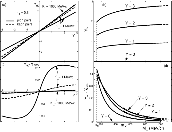
Figure 2: The YK rapidity, defined as $Y_{{}_{\rm YK}}=0.5\,\ln(1+v)/(1-v)$. Transverse flow $\eta_{f}=0.3$, solid lines – pions, dashed lines – kaons. a) Dependence of $Y_{{}_{\rm YK}}$ on the rapidity of the pair $Y$ for fixed $K_{\perp}$; b) dependence of $Y_{{}_{\rm YK}}$ on $M_{\perp}$ for fixed $Y$; c) dependence of the difference between $Y_{{}_{\rm YK}}$ and the rapidity of the point of maximal emissivity $Y_{{}_{\rm LSPS}}$ on $Y$ for fixed $K_{\perp}$; d) same as c) but dependence on $M_{\perp}$ for fixed $Y$.

To illustrate the main properties of the YKP radii we present here results obtained from a model study. The radii are calculated numerically using the formulae (17–19) and (20–23). As a model for the source the emission function of ref.[34] which is a special case of the emission function from ref.[24] is taken. It is given by the formula

$$S(x,K)=\frac{M_{\perp}\cosh(\eta-Y)}{{(2\pi)}^{3}\sqrt{2\pi{(\Delta\tau)}^{2}}}\exp\left[-\frac{K\cdot u(x)}{T}\right]\exp\left[-\frac{r^{2}}{2R^{2}}-\frac{{(\eta-\eta_{0})}^{2}}{2{(\Delta\eta)}^{2}}-\frac{{(\tau-\tau_{0})}^{2}}{2{(\Delta\tau)}^{2}}\right]\,.$$ (35)

The first part of this emission function describes the geometry of the freeze-out hypersurface. The second is a Lorentz invariant Boltzmann distribution which reflects the assumption of local thermal equilibrium at freeze-out. The last exponential describes the finite geometrical size of the source in the transverse direction, space-time rapidity and proper time. The motion of the different fluid elements of the source is expressed by the velocity field $u(x)$. Here we assume longitudinal expansion of the Bjorken type [35] and a linear transverse expansion profile. Then the components of $u(x)$ are given by:

$$u(x)=(\cosh\eta\,\cosh\eta_{t}(r),\,\sinh\eta_{t}(r)\frac{x}{r},\,\sinh\eta_{t}(r)\frac{y}{r},\,\sinh\eta\,\sinh\eta_{t}(r))$$ (36)

with

$$\eta=\frac{1}{2}\ln\frac{t+z}{t-z}$$ (37)

and

$$\eta_{t}(r)=\eta_{f}\frac{r}{R}$$ (38)

The parameter $\eta_{f}$ scales the strength of the transverse flow.

The temperature $T$ in the calculation was set to 140 MeV, the transverse geometric radius $R$ is 3 fm, the space-time rapidity width $\Delta\eta=1.2$, the average freeze-out proper time $\tau_{0}=3$ fm/c, and the mean proper emission duration $\Delta\tau=1$ fm/c. Calculations were done for pions ($m_{\pi}=139$ MeV) and kaons ($m_{K}=494$ MeV).

The behavior of the YK velocity in this model is plotted in Fig. 2 . The results are presented using the rapidities instead of velocities. The Yano-Koonin rapidity is connected with the YK velocity via the usual relation

$$Y_{{}_{\rm YK}}=\frac{1}{2}\ln\frac{1+v}{1-v}$$ (39)

Fig. 2a shows the dependence of the YK rapidity on the rapidity of the pair. The linear increase is a consequence of the assumed longitudinal expansion with a Bjorken flow profile. It is also seen that the lines corresponding to the pairs with higher transverse mass are closer to the diagonal. They reach the diagonal in the limit $M_{\perp}\to\infty$. This tendency is evident in Fig. 2b. The YK rapidity is sensitive mainly to the longitudinal rapidity of the pair, the dependence on its transverse mass being weaker. The $M_{\perp}$ dependences for pions and kaons almost coincide; the slight breaking of $M_{\perp}$ scaling is caused by the non-vanishing transverse flow [19].

The plots c) and d) of Fig. 2 show the difference between the YK rapidity and the rapidity of the point of maximal emissivity of the source for given pair rapidity and transverse mass. This difference is appreciable only in the region with non-zero pair rapidity and small $M_{\perp}$. But already in the region of measurements with kaons the difference is very small.

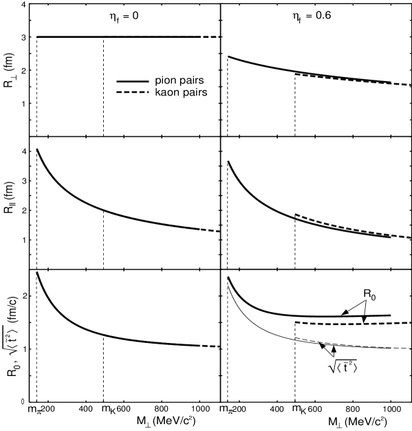
Figure 3: Dependences of the YKP radius parameters on $M_{\perp}$. Solid lines – pions, dashed lines – kaons. Left column: $\eta_{f}=0$, right column: $\eta_{f}=0.6$. The lines for $R_{0}$ in the case with the transverse flow are also compared to the real effective lifetime ${\left\langle{\tilde{t}}^{2}\right\rangle}^{\frac{1}{2}}$. Without transverse flow ${\left\langle{\tilde{t}}^{2}\right\rangle}^{\frac{1}{2}}$ coincides with $R_{0}$.

In Fig. 3 the characteristic behavior of the YKP radius parameters is plotted. The two columns correspond to different physical scenarios: the left one is without transverse flow while in the right one the value of $\eta_{f}$ is quite big ($\eta_{f}=0.6$). Before embarking on an interpretation of the dependences let us recall that the HBT radii measure the homogeneity lengths and not the dimensions of the whole fireball.

It is clearly seen that the strong transverse flow breaks the common $M_{\perp}$ scaling – the lines for pions and kaons do not coincide. Without the transverse flow the only parameter in the emission function is the transverse mass and the $M_{\perp}$ scaling is restored. The influence of transverse flow is most evident in the behavior of $R_{\perp}$. For $\eta_{f}=0$ there is no dynamics which could influence the transverse radius, hence it is given by the geometric transverse radius of the source. In the real experiment there could be another dynamical effects leading to the non-trivial $M_{\perp}$ dependence, e.g. temperature gradients. But the only yet known effect, within the class of thermal models, leading to the breaking of common $M_{\perp}$ scaling is the transverse flow.

The decrease of $R_{\parallel}$ is a result of the longitudinal dynamics with strong velocity gradient. The fluid element with given $z$-coordinate moves with the longitudinal velocity

$$v=\frac{z}{t}\,.$$ (40)

The particle with some longitudinal velocity is effectively produced by the fluid element with the same velocity and its surroundings with velocities within the thermal smearing. The thermal smearing in this way delimits for higher $M_{\perp}$ a smaller velocity interval than for lower $M_{\perp}$. According to eq.(40) the longitudinal radius decreases. Again, transverse flow destroys the common $M_{\perp}$ scaling.

The behavior of $R_{0}$ is related to the $M_{\perp}$ dependence of $R_{\parallel}$. It is given by the geometry of the freeze-out hypersurface. This source freezes out along the hyperbola in z-t diagram. Thus events at the freeze-out hypersurface with different longitudinal coordinates occur at different times and the longitudinal homogeneity length determines partially the effective emission duration (lifetime) [16, 24]. If the longitudinal homogeneity length vanishes (i.e. at large $M_{\perp}$), the lifetime is given by the geometric temporal term with width $\Delta\tau$.

In the case with transverse flow, the difference between $R_{0}$ and the effective emission duration is plotted too. For high $M_{\perp}$, $R_{0}$ is about 50% bigger than the real lifetime of the source, but note, that the assumed value of $\eta_{f}$ is rather high. For realistic cases we expect $\eta_{f}$ about 0.2 - 0.3. If the transverse flow vanishes, $R_{0}$ measures the lifetime exactly.

5 Conclusions

The Yano-Koonin-Podgoretskiĭ parametrisation of the two-particle correlation function has been presented. Comparing to the older and widely used Cartesian parametrisation it provides better insight into the dynamics of the source.

A great advantage is the direct measurement of the emission duration provided by $R_{0}$. The lifetime is the leading term in the model-independent expression for $R_{0}$ and it is measured with some small deviations arising from the non-vanishing transverse flow.

The fourth fit parameter, the YK velocity or YK rapidity, offers a possibility to study the longitudinal dynamics of the source. Its linear increase with the rapidity of the pair is a signal for a longitudinal expansion. On the other side, if $Y_{{}_{\rm YK}}$ does not depend on the pair rapidity, this is a signal for a source without longitudinal expansion, producing particles with all rapidities from a source at rest in the CM. Please note, that these statements are not based on model independent results but on the results of model studies within a class of thermal models.

Acknowledgements: We thank H. Appelshäuser, D. Ferenc, K. Kadija, J. Pišút and C. Slotta for stimulating and clarifying discussions. B.T. expresses his thanks to the organizers of the Workshop on Heavy Ion Collisions in Bratislava for the invitation and to the Dept. of Theor. Physics of Comenius University for kind hospitality. This work was supported by DAAD, DFG, NSFC, BMBF and GSI.

References

-
[1]
R. Hanbury-Brown, R.Q. Twiss:
Philos. Mag. 45 (1954), 633;
Nature 177 (1956), 27;
ibid 178 (1956), 1046 and 178 (1956), 1447. - [2] G. Goldhaber, S. Goldhaber, W. Lee, A. Pais: Phys. Rev. 120 (1960), 300.
- [3] M. Gyulassy, S.K. Kauffmann, L.W. Wilson: Phys. Rev. C 20 (1979), 2267.
- [4] D. Boal, C.K. Gelbke, B. Jennings, Rev. Mod. Phys. 62 (1990), 553.
- [5] W. Zajc: in Particle Production in Highly Excited Matter, (Eds. H.H. Gutbrod and J. Rafelski). Plenum Press, New York, 1993, p. 435.
- [6] S. Pratt, in Quark-Gluon Plasma 2, (Ed. R.C. Hwa). World Sci., Singapore 1995, p. 700.
- [7] U.A. Wiedemann: Acta Phys. Slov. 46 (1996), 567.
-
[8]
E. Shuryak: Phys. Lett. B 44 (1973), 387;
Sov. J. Nucl. Phys. 18 (1974), 667. -
[9]
S. Pratt: Phys. Rev. Lett. 53 (1984), 1219;
Phys. Rev. D 33 (1986), 1314. - [10] S. Chapman, U. Heinz: Phys. Lett. B 340 (1994), 250.
- [11] U.A. Wiedemann, U. Heinz: Resonance decay contributions to HBT correlation radii, Regensburg preprint TPR-96-14, nucl-th/9611031.
- [12] U.A. Wiedemann, U. Heinz: this volume.
-
[13]
J. Bolz et al.: Phys. Lett. B 300 (1993), 404 and
Phys. Rev D 47 (1993), 3860. - [14] B.R. Schlei et al.: Phys. Lett. B 376 (1996), 212.
- [15] U. Ornik et al.: Hydrodynamical analysis of symmetric nucleus-nucleus collisions at CERN/SPS energies. LAUR-96-1298, hep-ph/9604323.
- [16] S. Chapman, P. Scotto, U. Heinz: Heavy Ion Physics 1 (1995), 1.
- [17] U.A. Wiedemann, P. Scotto, U. Heinz: Phys. Rev. C 53 (1996), 918.
- [18] U. Heinz, B. Tomášik, U.A. Wiedemann, Y.-F. Wu: Phys. Lett. B 382 (1996), 181.
- [19] Y.-F. Wu, U. Heinz, B. Tomášik, U.A. Wiedemann: Yano-Koonin-Podgoretskiĭ Parametrisation of the HBT Correlator: A Numerical Study, Regensburg preprint TPR-96-12, nucl-th/9607044.
- [20] T. Csörgő: private communication.
- [21] A.N. Makhlin, Y.M. Sinyukov: Z. Phys. C 39 (1988), 69.
- [22] S. Chapman, P. Scotto, U. Heinz: Phys. Rev. Lett. 74 (1995), 4400.
- [23] S.V. Akkelin, Y.M. Sinyukov: Phys. Lett. B 356 (1995), 525.
- [24] T. Csörgő, B. Lörstad: Phys. Rev. C 54 (1996) 1390.
- [25] U. Heinz, B. Tomášik, U.A. Wiedemann, Y.-F. Wu: in Proceedings of the workshop Strangeness ’96, May 15.-17. 1996, Budapest, Hungary. special issue of the journal Heavy Ion Physics; nucl-th/9606041.
- [26] NA44 Coll., H. Beker et al.: Phys. Rev. Lett. 74 (1995), 3340.
-
[27]
NA35 Coll., T. Alber et al.: Z. Phys. C
66 (1995), 77;
NA35 Coll., T. Alber et al.: Phys. Rev. Lett. 74 (1995), 1303. - [28] T. Alber for the NA35 and NA49 Coll.: Nucl. Phys. A 590 (1995), 453c.
- [29] K. Kadija for the NA49 Coll.: in Quark Matter ’96, 20.-24.5.1996, Heidelberg, Germany, Ed. P. Braun-Munzinger et al., Nucl. Phys. A, in press.
- [30] M. Herrmann, G.F. Bertsch: Phys. Rev. C 51 (1995), 328.
- [31] T. Csörgő, S. Pratt: in Proceedings of the Workshop on Relativistic Heavy Ion Physics at Present and Future Accelerators, Budapest, 1991, (Eds. T. Csörgő et al.) MTA KFKI Press, Budapest, 1991, p. 75.
- [32] F. Yano, S. Koonin: Phys. Lett. B 78 (1978), 556.
- [33] M.I. Podgoretskiĭ : Sov. J. Nucl. Phys. 37 (1983), 272.
- [34] S. Chapman, J.R. Nix, U. Heinz: Phys. Rev. C 52 (1995), 2694.
- [35] J.D. Bjorken: Phys. Rev. D 27 (1983) 140.