Abstract: The classical Yang-Mills radiation computed in the McLerran-Venugopalan model is shown to be equivalent to the gluon bremsstrahlung distribution to lowest ($g^{6}$) order in pQCD. The classical distribution is also shown to match smoothly onto the conventional pQCD mini-jet distribution at a scale $k_{\perp}^{2}\sim\chi$, characteristic of the initial parton transverse density of the system. The atomic number and energy dependence of $\chi$ is computed from available structure function information. The limits of applicability of the classical Yang-Mills description of nuclear collisions at RHIC and LHC energies are discussed.

PACS numbers: 12.38.Bx,12.38.Aw,24.85.+p,25.75-q

1 Introduction

In this paper, we compare recent classical and quantal derivations of induced gluon radiation for applications to ultra-relativistic nuclear collisions. The classical distribution, based on the McLerran-Venugopalan model[1], was recently computed to order $g^{6}$ in Ref.[2]. The soft gluon bremsstrahlung distribution was computed via pQCD by Bertsch and Gunion in Ref.[3] within the Low-Nussinov approximation. Another quantal distribution, based on the Gribov-Levin-Ryzkin ladder approximation[4], was recently applied by Eskola et al[5]. Finally, there has been considerable recent effort to compute moderate $p_{\perp}$ (mini-jet) distributions based on the conventional collinear factorized pQCD approach[6, 7, 8].

Interest in the moderate $p_{\perp}$ gluon distributions arises in connection with estimates of the initial conditions and early evolution of the quark-gluon plasma formed in ultra-relativistic nuclear collisions at RHIC ($\surd s=200$ AGeV) and LHC ($\surd s=6500$ AGeV) energies. Until recently, the main source of mid-rapidity gluons was assumed to be copious mini-jet production as predicted via the conventional pQCD $gg\rightarrow gg$ processes[6, 7, 8]. However, in Refs.[1, 2] it was suggested that another important source of mid-rapidity gluons could be the classical Yang-Mills bremsstrahlung associated with the passage of two heavy nuclei through each other. In the conventional approach, beam jet bremsstrahlung is assumed to influence only the non-perturbative low transverse momentum beam jet regions. Beam jets are then typically modeled by pair production in Lund or Dual Parton Model strings. See for example Refs. [7, 8] and references therein.

The novel suggestion in [1] was that for sufficiently large $A$ nuclei and high energy, the initial nuclear parton density per unit area could become so high that the intrinsic transverse momentum of the partons, $\surd\chi\propto A^{1/6}\Lambda_{QCD}$, could extend into the mini-jet perturbative regime, $k_{\perp}\sim 2-4$ GeV. It was suggested that beam jet bremsstrahlung could even dominate that few GeV transverse momentum region because it is formally of lower order in $\alpha_{s}$ than mini-jet production. Such a new source of moderate $p_{\perp}$ partons would then significantly modify the early $\tau\sim 1/\surd\chi$ evolution and hence possibly modify many of the proposed signatures of the quark-gluon plasma in such reactions[9].

One of the aims of the present paper is to show in fact that the classical and quantal bremsstrahlung and mini-jet sources of mid-rapidity gluons are actually equivalent up to form factor effects over a continuous range of $p_{\perp}\sim\surd\chi$ regime. In addition we explore the limits of the validity of each approximation and compute numerically the energy and atomic number dependence of the McLerran-Venugopalan density parameter, $\chi$. This parameter is the total color charge squared per unit area of partons with rapidities exceeding some reference value.

The calculation of this paper checks that there is a region of overlap between the classical and quantum computation. The quantum calculation should be valid at large transverse momenta. The classical calculation is valid at momenta $\Lambda_{QCD}\ll k_{\perp}\ll\surd s$. Most of the gluons are produced in the region appropriate for the classical calculation. It is well known that perturbative calculations of gluon production are power law sensitive to an infrared cutoff. The classical computation has this infrared cutoff built into the calculation and may ultimately lead to a proper computation of gluon production. The region where we can compare the calculations is at $k_{\perp}$ much greater than this cutoff.

The plan of this paper is as follows: In section 2, we review the classical derivation of induced gluon radiation in the McLerran-Venugopalan model. We correct the treatment in [2] of the contact term in the classical equations of motion for a single nucleus. We extend further that derivation to treat properly the renormalization group corrections to the density parameter $\chi$. Those corrections[10] increase significantly the color charge squared per unit area relative to the contribution of the valence quarks thusfar considered [2, 11, 12]. We also correct omitted factors of 2 and $2\pi$ in the original computation[2].

In the third section, we review pQCD based derivations of induced gluon radiation[3]-[4]. We show that the classical result agrees with the quantal results of Bertsch and Gunion.[3] and also with the GLR formulation[4] if DGLAP evolution of the structure functions is assumed. We then compare the bremsstrahlung distribution to the mini jet distribution and show that while the latter dominates at high transverse momentum $p_{\perp}\gg\surd\chi$, the former dominates at $p_{\perp}\ll\surd\chi$. However, there is a continuous range of momenta $\sim\surd\chi$ where both results agree at the level of $20-40\%$.

In the fourth section, we compute the parameter $\chi$ of the McLerran-Venugopalan model. We find that due to the rapid rise of the small $x$ gluon structure functions, $\surd\chi$ approaches on the order of 1 GeV by LHC energies for $A\sim 200$. Possible implications and further extensions of this model conclude the paper.

2 Classical Yang-Mills Radiation

The basic assumption of the classical approach that follows is that the coupling strength is small at the scale

$$\Lambda^{2}={1\over{\pi R^{2}}}{{dN}\over{dy}}\gg\Lambda_{QCD}^{2}\;\;.$$ (1)

The parameter $\Lambda^{2}$ is the number density of gluons per unit rapidity per unit area. .

The gluon distribution was shown in Ref. [10] to solve an evolution equation which in various limits is the BFKL equation[13], the DGLAP equation[16], or its non-linear generalization[4]. In the ultra-relativistic domain, also the rate of change of the multiplicity per unit rapidity

$${{d^{2}N/dy^{2}}\over{dN/dy}}\sim\alpha_{s}$$ (2)

is small. The smallness of this parameter means that if we compute the gluon distribution in a small region $\Delta y\sim 1$ around $y=0$, then the source of those gluons is dominated by hard partons with rapidities much larger than 1. These hard partons can be integrated out of the effective action which describes the color field source at $y\sim 1$, and they lead to an effective external classical static source for the gluon field.

Since this can be done at any reference rapidity, the classical gluon field may be thought of as arising from a rapidity dependent classical source. For a single nucleus moving near the positive light cone, we have

$$D_{\mu}F^{\mu\nu}=g^{2}\delta^{\nu+}\rho(x^{-},x_{\perp})$$ (3)

with the source approximately independent of $x^{+}=(t+z)/\surd 2$. Two types of rapidity variables must be differentiated. In the classical equation of motion, the coordinate space rapidity is relevant as defined by

$$y=\ln 1/x^{-}=y_{proj}-\ln(x^{-}/x^{-}_{proj})\;\;,$$ (4)

and $x^{-}=(t-z)/\surd 2$. The momentum space rapidity is, on the other hand,

$$y={1\over 2}\ln(p^{+}/p^{-})$$ (5)

where

$$p^{\pm}={1\over\sqrt{2}}(p^{0}\pm p^{3})$$ (6)

are the conjugate momenta to $x^{\pm}$. For a hadron with $p^{+}=p^{+}_{proj}$, we define $x_{proj}^{-}=exp(-y_{proj})\sim 1/p^{+}_{proj}$.

The coordinate space rapidity is of the same order as the momentum space rapidity, since by the uncertainty principle $\Delta x^{-}\sim 1/p^{+}$. Qualitatively, these rapidities may thus be thought of as interchangeable. On the other hand, the classical equations of motion are described by coordinate space variables, and we must use the coordinate space rapidity.

In the McLerran-Venugopalan model, the source rapidity density

$$\rho(y,x_{\perp})\equiv x^{-}\rho(x^{-},x_{\perp})\;\;,$$ (7)

is assumed to be a stochastic variable which is integrated over with a Gaussian weight,

$$\int[d\rho]exp\left(-\int dyd^{2}x_{\perp}{1\over\mu^{2}(y)}{\rm Tr}\rho^{2}(y,x_{\perp})\right)\;\;.$$ (8)

This Gaussian assumption ignores correlations which we will see later are needed to regulate the infrared singularities. Here $\mu^{2}(y)$ is the average charge squared per unit rapidity per unit area scaled by $1/(N_{c}^{2}-1)$

$$\mu^{2}(y)={1\over{N_{c}^{2}-1}}{1\over{\pi R^{2}}}{{dQ^{2}}\over{dy}}$$ (9)

Note that this $\mu^{2}(y)$ specifies the rms fluctuations of the charge transverse density at a fixed rapidity. The quantity analogous to the rapidity independent $\mu$ used in [2] is the integrated transverse density of color charge arising from hard partons exceeding a reference rapidity. To emphasize this distinction we denote this quantity by

$$\chi(y)=\int_{y}^{y_{proj}}dy^{\prime}\mu^{2}(y^{\prime})\;\;.$$ (10)

This quantity will related below to the integrated gluon structure function.

The solution to the above equations may be found in the light cone gauge by assuming that

$$A^{\pm}=0\;\;,\;\;A^{i}=A^{i}(y,x_{\perp})$$

The index $i=1,2$ ranges over only the two-dimensional transverse coordinates. The field $A^{i}$ solves

$$-D_{i}{d\over{dy}}A^{i}=g^{2}\rho(y,x_{\perp})\;\;.$$ (11)

Equation (11) is solved by letting[10]-[11]

$$A^{i}(y,x_{\perp})={1\over i}\left(Pe^{i\int_{y_{proj}}^{y}dy^{\prime}\Lambda(y^{\prime},x_{\perp})}\right)^{\dagger}\nabla^{i}\left(Pe^{i\int_{y_{proj}}^{y}dy^{\prime}\Lambda(y^{\prime},x_{\perp})}\right)$$ (12)

In this equation, $P$ denotes path ordering along the integration in rapidity.

If we now change variables (with unit determinant in the integration over sources)

$$\left(Pe^{i\int_{y_{proj}}^{y}dy^{\prime}\Lambda(y^{\prime},x_{\perp})}\right)\rho\left(Pe^{i\int_{y_{proj}}^{y}dy^{\prime}\Lambda(y^{\prime},x_{\perp})}\right)^{\dagger}\rightarrow\rho\;\;,$$ (13)

then $\Lambda$ is seen to obey the two dimensional Poisson’s equation

$$-\nabla^{2}_{\perp}\Lambda(y,x_{\perp})=g^{2}\rho(y,x_{\perp})$$ (14)

Note that due to the expected slow variation of the source density as a function of rapidity, the field is almost constant in $y$. At zero rapidity, therefore, the field may be taken approximately as

$$A_{i}(x^{-},x_{\perp})=\theta(x^{-})\alpha_{i}^{+}(x_{\perp})$$ (15)

where

$$\alpha_{i}^{+}(x_{\perp})={1\over i}\left(Pe^{i\int_{y_{proj}}^{0}dy^{\prime}\Lambda(y^{\prime},x_{\perp})}\right)^{\dagger}\nabla_{i}\left(Pe^{i\int_{y_{proj}}^{0}dy^{\prime}\Lambda(y^{\prime},x_{\perp})}\right)$$ (16)

This is the non-abelian Weizsäcker-Williams field of the projectile nucleus which must still be averaged over the ensemble (8).

In order to generalize the above solution to the case of two colliding nuclei, we use the same variables as above for the projectile nucleus propagating in the $+z$ direction. For the target nucleus propagating in the $-z$ direction, we use the rapidity variable

$$y=-y_{cm}+\ln(x_{0}^{+}/x^{+})$$ (17)

Here we denote the projectile rapidity with the center of mass rapidity as, $y_{cm}=y_{proj}$. We will also henceforth use the index $+$ to refer to $y>0$ and $-$ to $y<0$, when no confusion will arise with respect to light cone variable indices.

In the neighborhood of $y=0$, we can ignore the small rapidity dependence of the fields. The solution to the equations of motion in the

$$x^{+}A^{-}+x^{-}A^{+}=0$$ (18)

gauge is approximately given by

$$A^{\pm}=\pm x^{\pm}\theta(x^{+})\theta(x^{-})\beta(\tau,x_{\perp})$$ (19)

and

$$A_{i}=\theta(x^{+})\theta(x^{-})\alpha_{i}^{3}(\tau,x_{\perp})+\theta(-x^{+})\theta(x^{-})\alpha^{+}_{i}(x_{\perp})+\theta(x^{+})\theta(-x^{-})\alpha^{-}_{i}(x_{\perp})$$ (20)

Here $\tau=\sqrt{t^{2}-z^{2}}$ is a boost covariant time variable. (Note that the above notation corresponds to $\beta=\alpha$ and $\alpha^{3}_{i}=\alpha_{i\perp}$ of [2].)

The fields

$$\alpha^{\pm}_{i}={1\over i}\left(Pe^{i\int_{\pm y_{cm}}^{0}dy^{\prime}\Lambda(y^{\prime},x_{\perp})}\right)^{\dagger}\nabla_{i}\left(Pe^{i\int_{\pm y_{cm}}^{0}dy^{\prime}\Lambda(y^{\prime},x_{\perp})}\right)$$ (21)

where

$$-\nabla^{2}_{\perp}\Lambda(y,x_{\perp})=g^{2}\rho(y,x_{\perp})$$ (22)

and where

$$\rho(y,x_{\perp})=\theta(y)\rho^{+}(y,x_{\perp})+\theta(-y)\rho^{-}(y,x_{\perp})$$ (23)

Notice that in this solution, the fields $\alpha_{i}^{\pm}$ are two dimensional gauge transforms of vacuum fields. Their sum is of course not a gauge transform of vacuum fields, and therefore the solution cannot continue into the region $x^{\pm}>0$. There is in fact a singularity in the solution at $x^{+}=0$ and $x^{-}=0$, at $x^{+}=0$ for $x^{-}>0$, and at $x^{-}=0$ for $x^{+}>0$. For $x^{\pm}>0$, the form of the fields chosen above solves the classical equations of motion. In this region, the solution is a boundary values problem with the boundary values specified on the edge of the forward light cone.

To determine these boundary values, we solve

$$D_{\mu}F^{\mu\pm}=g^{2}\rho$$ (24)

and

$$D_{\mu}F^{\mu i}=0$$ (25)

First we find the singularities of Eqn. 25. In this equation, there is a $\delta(x^{+})\delta(x^{-})$ singularity, that is a singularity at the tip of the light cone. The absence of such a singularity requires that

$$\alpha_{i}^{3}\mid_{\tau=0}=\alpha^{+}_{i}(x_{\perp})+\alpha^{-}_{i}(x_{\perp})$$ (26)

There are also singularities of the form $\delta(x^{\pm})$ for $x^{\mp}>0$. The absence of these singularities requires $\alpha^{3}$ be analytic as $\tau\rightarrow 0$.

The solution for the Eqn. 24 is a little trickier since there are some potentially singular contact terms. It can be shown that if the fields $\alpha^{\pm}_{i}$ are properly smeared in rapidity so that they really solve the equations of motion in the backwards light cone, then all such contact terms disappear. We find that $\beta$ must be analytic at $\tau=0$ and that

$$\beta\mid_{\tau=0}={i\over 2}[\alpha^{+}_{i},\alpha^{-}_{i}]\;\;.$$ (27)

The boundary conditions are precisely those of Ref. [2]. They have been rederived here to properly account for any singularities in arising from contact terms in the equations of motion. These contact terms when properly regulated do not affect the boundary conditions.

We now construct an approximate solution of the equations of motion in the forward light cone. We do this by expanding around the solution which is a pure two dimensional gauge transform of vacuum which is closest to $\alpha^{+}+\alpha^{-}$. To do this, we introduce the projectile and target source charge per unit area at a reference rapidity $y$ as

$$q^{\pm}(y,x_{\perp})=\pm\int_{y}^{\pm y_{cm}}dy^{\prime}\rho(y^{\prime},x_{\perp})$$ (28)

and

$$\eta^{\pm}(y,x_{\perp})=\pm\int_{y}^{\pm y_{cm}}dy^{\prime}\Lambda(y^{\prime},x_{\perp})$$ (29)

Note that

$$\langle q^{\pm}_{a}(y,x_{\perp})q^{\pm}_{b}(y,x_{\perp}^{\prime})\rangle=\chi^{\pm}(y)\delta_{a,b}\delta^{2}(x_{\perp}-x_{\perp}^{\prime})$$ (30)

in terms of $\chi^{\pm}(y)$ defined as in (10).

By direct computation, as in [2]

$$\alpha_{i}^{\pm}=\nabla_{i}\eta^{\pm}-{i\over 2}[\eta^{\pm},\nabla_{i}\eta^{\pm}]$$ (31)

and

$$\eta^{\pm}=g^{2}{1\over{\nabla^{2}_{\perp}}}q^{\pm}$$ (32)

The sum of $\alpha^{+}+\alpha^{-}$ can be written as a pure two dimensional gauge transform of vacuum plus a correction as

$$\alpha^{+}_{i}+\alpha^{-}_{i}=\alpha_{i}^{0}+\delta\alpha_{i}^{0}$$ (33)

where

$$\alpha_{i}^{0}=\nabla_{i}(\eta^{+}+\eta^{-})-{i\over 2}[\eta^{+}+\eta^{-},\nabla_{i}(\eta^{+}+\eta^{-})]$$ (34)

and where

$$\delta\alpha^{0}_{i}={i\over 2}\{[\eta^{-},\nabla_{i}\eta^{+}]+[\eta^{+},\nabla_{i}\eta^{-}]\}$$ (35)

This decomposition into a gauge transform of the vacuum is accurate up to and including order $g^{4}$.

Now we expand $\alpha_{i}^{3}=\alpha^{0}_{i}+\delta\alpha^{3}_{i}(\tau,x_{\perp})$. Both $\delta\alpha^{3}$ and $\beta$ are the small fluctuation fields corresponding to radiation. We find that $\delta\alpha^{3}$ and $\beta$ solve exactly the same equations as were incorrectly derived in Ref. [2]. So even though the original derivation was incorrect, the final result remains fortunately valid.

In Eqn. 42 [2], a factor of $2\pi$ was however omitted, and as well in Eqns. 45, 47, 49 and 50. In addition, in going from the first of Eqns. 49 to the second, a factor of 1/2 from the trace was omitted.

The final result corrected for the above factors and generalized to include the source of hard gluons is

$${{dN}\over{dyd^{2}k_{\perp}}} = \pi R^{2}{{2g^{6}\chi^{+}(y)\chi^{-}(y)}\over{(2\pi)^{3}}}{{N_{c}(N_{c}^{2}-1)}\over{k_{\perp}^{2}}}\int{{d^{2}q_{\perp}}\over{(2\pi)^{2}}}{1\over{q_{\perp}^{2}({\bf q}_{\perp}-{\bf k}_{\perp})^{2}}}$$ (36)

$$= \pi R^{2}{{2g^{6}\chi^{+}(y)\chi^{-}(y)}\over{(2\pi)^{4}}}{{N_{c}(N_{c}^{2}-1)}\over k_{\perp}^{4}}{L}(k_{\perp},\lambda)\;\;.$$

The ${\bf q}_{\perp}=0$ and ${\bf q}_{\perp}={\bf k}_{\perp}$ divergences arise in the above classical derivation because of the neglect of correlations in the sources ensemble. A finite logarithmic factor , ${L}(k_{\perp},\lambda)$, is obtained only if we include a finite color neutralization correlation scale, $\lambda$.

This scale arises from dynamical screening effects and may be seen in models such as the onium valence quark model of Kovchegov[11] as developed in [12]. In the classical calculation, this cutoff appears after averaging over various values of the background charge density.[10] The cutoff scale turns out to be $\lambda\sim\alpha\surd\chi$. Below this cutoff scale, the factors of $1/k_{\perp}^{2}$ moderate and become of order $\ln(k_{\perp})$. This cutoff scale acts somewhat like a Debye mass, although this is not quite the case since the logarithmic dependence implies power law fall off in coordinate space whereas a Debye mass corresponds to exponential decay. In any case, for evaluating ${L}(k_{\perp},\lambda)$ at $k_{\perp}>>\lambda$ the precise form of the cutoff is unimportant, only that the $1/k_{\perp}^{2}$ singularities in the integrand are tempered at some scale. This is because logarithmically divergent integrals are insensitive in leading order to the precise form of the cutoff. The generic form of the logarithmic factor is therefore expected to be of the form

$${L}(k_{\perp},\lambda,y) = k_{\perp}^{2}\int{{d^{2}{\bf q}_{\perp}}\over{2\pi}}{{\cal F}(y,q_{\perp}^{2}){\cal F}(y,({\bf q}_{\perp}-{\bf k}_{\perp})^{2})\over{q_{\perp}^{2}({\bf q}_{\perp}-{\bf k}_{\perp})^{2}}}$$ (37)

where ${\cal F}$ is a suitable form factor. In [3] a dipole form factor was considered. A gauge invariant screening mass was considered in [14]. Such dipole form factors lead to

$${L}(k_{\perp},\lambda) = k_{\perp}^{2}\int{{d^{2}{\bf q}_{\perp}}\over{2\pi}}{1\over{(q_{\perp}^{2}+\lambda^{2})(({\bf q}_{\perp}-{\bf k}_{\perp})^{2}+\lambda^{2})}}\approx\log(k_{\perp}^{2}/\lambda^{2})\;\;,$$ (38)

where the logarithmic form is remarkably accurate for $k_{\perp}/\lambda>2$. A finite but nonlogarithmic form of $L$ can also arise if other functional forms for the form factors are considered as in [11, 12].

It is also important to stress that in any case, the above classical derivation neglected nonlinearities that can be expected to distort strongly the above perturbative solution in the $k_{\perp}^{2}<\alpha^{2}\chi$ region. Thus, the solution should not be extended below $\lambda\sim\alpha\surd\chi$ in any case. In future studies, it will be important to investigate just how the full nonlinear Yang-Mills equations regulate these infrared divergences.

2.1 Classical Color Current Fluctuations

For two colliding nuclei the effective classical source current for mid-rapidity gluons is assumed to be

$$j^{\mu}_{a}(x)=\delta^{\mu+}\delta(x^{-})q^{+}_{a}(0,{\bf x}_{\perp})+\delta^{\mu-}\delta(x^{+})q^{-}_{a}(0,{\bf x}_{\perp})$$ (39)

where $\langle q^{\pm}\rangle=0$ but the ensemble averaged squared color charge density of each of the $N_{c}^{2}-1$ components is given by $\chi^{\pm}(0)$ as in (30).

In ref.[11, 12], $\chi$ was estimated using the valence quark density and with the classical color density interpreted as a color transition density associated with the radiation of a color $a$ gluon

$$q^{a}({\bf x}_{\perp})=\sum_{n=1}^{N}(T^{a}_{n})_{c^{\prime},c}\delta^{2}({\bf x}_{\perp}-{{\bf x}_{\perp}}_{n})$$ (40)

where the sum is over the valence quarks, and $T^{a}_{n}$ is a generator of dimension $d_{n}$ appropriate for parton $n$. In this interpretation, products of color densities involve matrix multiplication and the ensemble average leads to a trace associated with averaging over all initial colors of the valence partons and a summing over all final colors. Therefore

$$\langle q_{i}^{a}({\bf x}_{\perp})\rangle=0$$ (41)

since $TrT^{a}=0$ in any representation while

$$\langle q^{a}({\bf x}_{\perp})q^{b}({\bf x}_{\perp}^{\prime})\rangle=\sum_{n=1}^{N}\frac{1}{d_{n}}Tr(T^{a}_{n}T^{b}_{n})n({\bf x}_{\perp})\delta^{2}({\bf x}_{\perp}-{{\bf x}_{\perp}}^{\prime})$$ (42)

where $n({\bf x}_{\perp})=\langle\delta({\bf x}_{\perp}-{\bf x}_{\perp}(n))\rangle$ is the transverse density of partons of type $n$. From now on we assume identical projectile and target combinations and fix $y=0$ so that we can drop the distinction between $\pm$ sources and the rapidity variable.

Taking into account both the valence quark and hard gluon contributions in the nuclear cylinder approximation used in [2], the relevant $\chi=\chi^{\pm}(0)$ parameter is therefore given by

$$\chi=\frac{1}{\pi R^{2}}\left(\frac{N_{q}}{2N_{c}}+\frac{N_{c}\;N_{g}}{N_{c}^{2}-1}\right)=\frac{1}{\pi R^{2}}(C_{F}N_{q}+C_{A}N_{g})/d_{A}$$ (43)

where the transverse density of quarks is $n_{q}({\bf x}_{\perp})=N_{q}/\pi R^{2}$ and the gluon transverse density is $n_{g}({\bf x}_{\perp})=N_{g}/\pi R^{2}$,

Because this interpretation allows for complex color (transition) densities that do not arise in the classical limit, it is useful to show that it can also be derived from a more conventional classical Yang-Mills treatment. For that purpose we use the Wong formulation of classical YM kinetic theory [15]. In that formulation, the parton phase space is enlarged to incorporate a classical charge vector $\Lambda^{a}(\tau)$ in addition to the usual $(x^{\mu}(\tau),p^{\mu}(\tau)=mu^{\mu}(\tau))$ phase space coordinates. The phase space density, $f$, obeys the Liouville equation

$$\frac{d}{d\tau}f(x(\tau),p(\tau),\Lambda(\tau))=0$$ (44)

with $dx^{\mu}/d\tau=u^{\mu}$ and

$$m\frac{du^{\mu}}{d\tau} = gu_{\nu}F^{\mu\nu}_{a}\Lambda^{a}$$

$$\frac{d\Lambda^{a}}{d\tau} = gf^{abc}u_{\mu}A^{\mu b}\Lambda^{c}=-i\left({\cal T}^{b}\theta^{b}\right)_{ac}\Lambda^{c}\;\;.$$ (45)

where $({\cal T}^{b})_{ac}=if^{abc}$ are the generators in the adjoint representation and $\theta^{b}=gu_{\mu}A^{\mu b}$. The color current $gj^{\mu a}(x)$ in this kinetic theory is computed via

$$j^{\mu a}(x)=\int d\tau u^{\mu}(\tau)\Lambda^{a}(\tau)\delta^{4}(x-x(\tau))$$ (46)

The color charge vector precesses around the local $A^{\mu a}$ field but its magnitude remains constant. Its length is fixed by the specified color Casimir $C_{2}=\sum_{a}\Lambda_{a}^{2}$. In the ultra-relativistic case with $p^{z}/p_{0}\approx 1$, the current reduces to eq.(39) with the transverse density

$$q^{a}({\bf x}_{\perp})=\sum_{n}U_{ac}\Lambda^{c}_{n}(\tau_{0})\delta^{2}({\bf x}_{\perp}-{{\bf x}_{\perp}}_{n})$$ (47)

where the unitary $U=P\exp\{-ig\int_{0}^{1}ds{\cal T}^{b}u_{\mu}A^{\mu b}(x(s))\}$ accounts for the color precession along the parton trajectory. The ensemble average in this formulation involves an integration over the initial colors $\Lambda^{a}_{n}(\tau_{0})$ with a measure

$$d\Lambda_{n}\propto\prod_{c=1}^{d_{A}}d\Lambda^{c}_{n}\delta(\Lambda^{a}_{n}\Lambda^{a}_{n}-C_{2n})$$ (48)

normalized such that $\int d\Lambda_{n}=1$ and thus

$$\int d\Lambda_{n}\Lambda^{a}_{n}\Lambda^{b}_{n}=\delta^{ab}C_{2n}/d_{A}$$ (49)

Because $U$ is unitary, this leads to the same expression for the color charge squared correlation parameter $\chi$ as eq.(43).

2.2 Yang-Mills Radiation Distribution

Inserting the above expression for $\chi$ into the classical formula for radiation, we obtain

$$\frac{dN}{dyd^{2}k_{\perp}} = \frac{1}{\pi R^{2}}\left(\frac{N_{q}}{2N_{c}}+\frac{N_{c}\;N_{g}}{N_{c}^{2}-1}\right)^{2}\frac{2g^{6}}{(2\pi)^{3}}\frac{N_{c}(N_{c}^{2}-1)}{k_{\perp}^{2}}\int\frac{d^{2}{\bf q}_{\perp}}{(2\pi)^{2}}\frac{1}{q_{\perp}^{2}({\bf q}_{\perp}-{\bf k}_{\perp})^{2}}$$ (50)

$$= \frac{1}{\pi R^{2}}\left(C_{F}N_{q}+C_{A}N_{g})\right)^{2}\frac{1}{d_{A}}\frac{2g^{6}N_{c}}{(2\pi)^{4}}\frac{1}{k_{\perp}^{4}}{L}(k_{\perp},\lambda)$$

If only valence quarks are included then this reduces to

$$\frac{dN}{dyd^{2}k_{\perp}} = \frac{N_{q}^{2}}{\pi R^{2}}\left(\frac{2g^{6}N_{c}}{(2\pi)^{4}}\right)\left(\frac{C_{F}^{2}}{d_{A}}\right)_{el}\frac{1}{k_{\perp}^{4}}{L}(k_{\perp},\lambda)$$ (51)

In the opposite limit, if only hard glue is included, the radiation distribution reduces to

$$\frac{dN}{dyd^{2}k_{\perp}} = \frac{N_{g}^{2}}{\pi R^{2}}\left(\frac{2g^{6}N_{c}}{(2\pi)^{4}}\right)\left(\frac{C_{A}^{2}}{d_{A}}\right)_{el}\frac{1}{k_{\perp}^{4}}{L}(k_{\perp},\lambda)$$ (52)

Note that the color factor in the second brackets marked $el$ is that associated with the elastic scattering of two partons

$$C^{el}_{nm}=\left(\frac{1}{d_{n}}TrT^{a}_{n}T^{b}_{n}\right)\;\left(\frac{1}{d_{m}}TrT^{a}_{m}T^{b}_{m}\right)=\frac{C_{2n}C_{2m}}{d_{A}}\;\;,$$ (53)

so that $C^{el}=2/9,9/8$ for $qq,gg$. The elastic Rutherford cross section is in this approximation

$$\sigma^{el}_{nm}=\frac{g^{4}C^{el}_{nm}}{(2\pi)^{2}}\int\frac{d^{2}q_{\perp}}{q_{\perp}^{4}}=\int dt\frac{\pi\alpha^{2}}{t^{2}}\frac{4C_{2n}C_{2m}}{d_{A}}\;\;.$$ (54)

The infrared divergence is regulated by the color screening scale $\lambda$ or form factors as in [3].

The geometrical Glauber factor in Eqns. ( 51,52) counts the average number of binary parton-parton collisions per unit area in $b=0$ collisions of cylindrical nuclei. More generally,

$$T^{nm}_{AB}({\bf b})=\frac{1}{\sigma_{nm}}\int d^{3}x\rho_{n/A}({\bf x})\int dz_{B}\;\sigma_{nm}\rho_{m/B}({\bf x}_{\perp}-{\bf b},z_{B})$$ (55)

For $b=0$ collisions of cylindrical nuclei this reduces to

$$T^{nm}(0)=\frac{N_{n}N_{m}}{\pi R^{2}}$$ (56)

Therefore we can write

$$\frac{dN}{dyd^{2}k_{\perp}} = T^{nm}(0)\frac{d\sigma^{nm\rightarrow g}}{dyd^{2}k_{\perp}}$$ (57)

where

$$\frac{d\sigma^{nm\rightarrow g}}{dyd^{2}k_{\perp}} = C^{el}_{nm}\left(\frac{2g^{6}N_{c}}{(2\pi)^{3}}\right)\frac{1}{k_{\perp}^{2}}\int\frac{d^{2}{\bf q}_{\perp}}{(2\pi)^{2}}\frac{1}{q_{\perp}^{2}({\bf q}_{\perp}-{\bf k}_{\perp})^{2}}\;\;.$$ (58)

3 Quantum Radiation

3.1 pQCD Bremsstrahlung

We compare (58) with the quantum radiation formula derived in [3]. In the $A^{+}=0$ gauge and for gluon kinematics $k=[xP^{+},k_{\perp}^{2}/xP^{+},{\bf k}_{\perp}]$ with $x\ll 1$, the three dominant diagrams sum in the small momentum transfer limit to

$$iM({nm\rightarrow g(k,\epsilon,c)})=[T_{n}^{a},T^{c}_{n}]T^{a}_{m}\left(\frac{2g^{2}s}{q_{\perp}^{2}}\right)\left(2g\epsilon_{\perp}\cdot\left\{\frac{{\bf k}_{\perp}}{k_{\perp}^{2}}-\frac{{\bf k}_{\perp}-{\bf q}_{\perp}}{({\bf k}_{\perp}-{\bf q}_{\perp})^{2}}\right\}\right)$$ (59)

Taking the square and averaging over initial and summing over final colors, one finds that

$$\frac{d\sigma}{dq_{\perp}^{2}dyd^{2}k_{\perp}} = \left(\frac{C^{el}_{nm}4\pi\alpha^{2}}{t^{2}}\right)\left(\frac{\alpha N_{c}}{\pi^{2}}\frac{q_{\perp}^{2}}{k_{\perp}^{2}({\bf k}_{\perp}-{\bf q}_{\perp})^{2}}\right)$$ (60)

$$= \frac{d\sigma^{el}_{nm}}{dq_{\perp}^{2}}\frac{dN}{dyd^{2}k_{\perp}}\;\;.$$

This is the basic factorized form of the soft QCD radiation associated with elastic scattering. Integrating over the elastic momentum transfer $q_{\perp}$ yields

$$\frac{d\sigma}{dyd^{2}k_{\perp}} = \int\frac{d^{2}{\bf q}_{\perp}}{\pi}\left(\frac{C^{el}_{nm}4\pi\alpha^{2}}{q_{\perp}^{4}}\right)\left(\frac{\alpha N_{c}}{\pi^{2}}\frac{q_{\perp}^{2}}{k_{\perp}^{2}({\bf k}_{\perp}-{\bf q}_{\perp})^{2}}\right)$$ (61)

$$= C^{el}_{nm}\frac{2g^{6}N_{c}}{(2\pi)^{3}}\frac{1}{k_{\perp}^{2}}\int\frac{d^{2}{\bf q}_{\perp}}{(2\pi)^{2}}\frac{1}{q_{\perp}^{2}({\bf k}_{\perp}-{\bf q}_{\perp})^{2}}$$

This is exactly the same as the classical result in (58).

In Ref. [3] the $\pi\pi\rightarrow g$ cross section was computed taking a dipole form factor into account with the result

$$\frac{d\sigma^{\pi\pi\rightarrow g}}{dydk_{\perp}^{2}}=\left(\frac{C_{A}\alpha^{3}}{\pi^{2}k_{\perp}^{2}}\right)\int\frac{d^{2}{\bf q}_{\perp}}{(2\pi)^{2}}\frac{2^{2}F_{\pi}(q_{\perp}^{2})F_{\pi}(({\bf q}_{\perp}-{\bf k}_{\perp})^{2})}{q_{\perp}^{2}({\bf q}_{\perp}-{\bf k}_{\perp})^{2}}$$ (62)

where

$$F_{\pi}(q^{2})=\frac{4q^{2}}{4q^{2}+m_{\rho}^{2}}$$ (63)

Again we can read off the elementary $qq\rightarrow g$ cross section by dividing by the number of parton pairs $N_{q}^{2}=4$ in this reaction and neglecting interference by setting $F_{\pi}=1$. This leads to

$$\frac{d\sigma^{qq\rightarrow g}}{dydk_{\perp}^{2}}=\frac{1}{4}\left(\frac{2g^{6}N_{c}}{(2\pi)^{3}}\right)\frac{1}{k_{\perp}^{2}}\int\frac{d^{2}{\bf q}_{\perp}}{(2\pi)^{2}}\frac{1}{q_{\perp}^{2}({\bf q}_{\perp}-{\bf k}_{\perp})^{2}}$$ (64)

where the first factor 1/4 is just the large $N_{c}$ limit of $C^{el}_{qq}\rightarrow 1/4$ used implicitly in eq.(17) of [3].

3.2 Comparison with GLR formula

It is also of interest to connect the classical YM formula with the $pp\rightarrow g$ formula of Gribov, Levin, and Ryskin (GLR)[4]and used recently in ref.[5]to compute mid-rapidity gluon production at LHC energies:

$$\frac{d\sigma}{dyd^{2}{\bf k}_{\perp}} = K_{N}\frac{\alpha N_{c}}{\pi^{2}k_{\perp}^{2}}\int d^{2}{\bf q_{\perp}}\frac{f(x_{1},q_{\perp}^{2})f(x_{2},({\bf k}_{\perp}-{\bf q_{\perp}})^{2})}{q_{\perp}^{2}({\bf k}_{\perp}-{\bf q_{\perp}})^{2}}\;\;,$$ (65)

where

$$f(x,Q^{2})=\frac{d}{d\log Q^{2}}xG(x,Q^{2})$$ (66)

and

$$x_{1}\approx x_{2}\approx x_{\perp}\equiv k_{\perp}/\sqrt{s}$$ (67)

are fractional momenta which are assumed to be small. In this relation, the radiation resulting from the fusion of two off-shell $y_{1}\sim y_{2}\sim 0$ gluons is estimated. Unfortunately, there is variation in the literature as to the magnitude of the factor $K_{N}$ [4]. This is partly due to variations in the definition of $f(x,Q^{2})$. We find below that in order to reproduce the perturbative QCD and classical Yang-Mills result, eq.(61,58), we must take

$$K_{N}=\frac{(2\pi)^{2}}{N^{2}_{c}-1}\approx 5\;\;.$$ (68)

From private communication with E. Levin, this factor is required if $f$ is defined as in ref.[5] via (66). This implies that the results quoted for the BFKL contribution to minijets in [5] taking $K_{N}=1$ are approximately a factor 5 too small. With the value in eq.(68), the BFKL and conventional mini-jet rates would coincide more closely. In section 3.3 we argue that at least in the asymptotic domain these distributions should in fact coincide over a range of $k_{\perp}\sim\surd\chi$.

To compare to the GLR formula with the classical result, we approximate the $Q^{2}$ evolution using DGLAP evolution[16]

$$f(x,Q^{2})=\frac{dxG(x,Q^{2})}{d\log Q^{2}}\approx\frac{\alpha}{2\pi}\int_{x}^{1}\frac{dx^{\prime}}{x^{\prime}}\;G(x^{\prime},Q^{2})\;xP_{g\rightarrow g}(x/x^{\prime})\;\;.$$ (69)

In the small $x$ semi-classical domain

$$\;\;P_{gg}(x)\approx 2N_{c}/x$$ (70)

Therefore, we have the approximate relation at high $Q^{2}$

$$f(x,Q^{2})\approx\frac{\alpha N_{c}}{\pi}\int_{x}^{1}\;dx^{\prime}\;G(x^{\prime},Q^{2})=\frac{\alpha N_{c}}{\pi}N_{g}(x,Q^{2})$$ (71)

Consequently, from (66,71)

$$\frac{d\sigma}{dyd^{2}{\bf k}_{\perp}} = K_{N}\frac{\alpha N_{c}}{\pi^{2}k_{\perp}^{2}}\int d^{2}{\bf q_{\perp}}\frac{d\;xG}{dq_{\perp}^{2}}\;\left(\frac{d\;xG}{dq_{\perp}^{\prime 2}}\right)_{({\bf k}_{\perp}-{\bf q_{\perp}})^{2}}$$

$$\approx K_{N}\frac{\alpha N_{c}}{\pi^{2}k_{\perp}^{2}}\frac{\alpha^{2}N_{c}^{2}}{\pi^{2}}\int d^{2}{\bf q_{\perp}}\frac{N_{g}(x_{1},q_{\perp}^{2})N_{g}(x_{2},({\bf k}_{\perp}-{\bf q_{\perp}})^{2})}{q_{\perp}^{2}({\bf k}_{\perp}-{\bf q_{\perp}})^{2}}$$

Equation (LABEL:glr2) reduces to the classical expression (52) if we approximate the integral by factoring out the integrated gluon numbers at the average scale, $\sim k_{\perp}^{2}$, divide by $\pi R^{2}$, and take the normalization factor $K_{N}$ from (68).

3.3 Matching $2\rightarrow 3$ to $2\rightarrow 2$

Up to this point, we have shown that the classical and quantum bremsstrahlung formulas agree for the $2\rightarrow 3$ process up to specific form factors. The problem addressed in this section is the relationship between the bremsstrahlung spectrum and the mini-jet spectrum based on the pQCD factorized $2\rightarrow 2$ processes. Recall[6] the factorized differential cross section for two gluon jet production with transverse momenta , $\pm{\bf k}_{\perp}$, and rapidities $y_{1}$ and $y_{2}$, is given by

$${{d\sigma^{AB\rightarrow g_{1}g_{2}X}}\over{dy_{1}dy_{2}d^{2}{\bf k}_{\perp}}}=K\;x_{1}G_{A}(x_{1},k_{\perp}^{2})x_{2}G_{B}(x_{2},k_{\perp}^{2})\frac{1}{\pi}\frac{d\sigma^{gg\rightarrow gg}}{dt}\;\;,$$ (73)

where $x_{1}=x_{\perp}(\exp(y_{1})+\exp(y_{2}))$ and $x_{2}=x_{\perp}(\exp(-y_{1})+\exp(-y_{2}))$, with $x_{\perp}=k_{\perp}/\surd s$, and where the pQCD $gg\rightarrow gg$ cross section for scattering with $t=-k_{\perp}^{2}(1+\exp(y_{2}-y_{1}))$ and $y_{2}-y_{1}=y$ is given by

$$\frac{d\sigma^{gg}}{dt} = C^{el}_{gg}\frac{4\pi\alpha^{2}}{k_{\perp}^{4}}\frac{(1+e^{y}+e^{-y})^{3}}{(e^{y/2}+e^{-y/2})^{6}}\;\;.$$ (74)

This reduces to the naive Rutherford expression eq.(54) only if the unobserved gluon has a rapidity $|y|\ \raisebox{2.75pt}{$>$}\raisebox{-2.75pt}{$\sim$}\ 3$. For $|y|\ \raisebox{2.75pt}{$<$}\raisebox{-2.75pt}{$\sim$}\ 1$, the exact form (74) is $27/64\approx 0.42$ smaller than the Rutherford approximation.

We concentrate here only on the dominant gluon-gluon contribution for symmetric systems, $A+A$, with $G=G_{A}$. The inclusive gluon jet production cross section is obtained by integrating over $y_{2}$ with $y_{1}=y$ and $k_{\perp}$ fixed. For an observed midrapidity gluon with $y=0$, $-y^{*}<y_{2}<y^{*}$, where $\exp(-y^{*})=x_{\perp}/(1-x_{\perp})$, we must evaluate

$$I(x_{\perp},k_{\perp}^{2}) = \int_{-y^{*}}^{y^{*}}dy_{2}\;x_{1}G(x_{1},k_{\perp}^{2})x_{2}G(x_{2},k_{\perp}^{2})\frac{(1+e^{y_{2}}+e^{-{y_{2}}})^{3}}{(e^{y_{2}/2}+e^{-y_{2}/2})^{6}}\;\;.$$ (75)

In the Rutherford approximation, implicit in the classical approximation, we neglect the $y$ dependence of (74) and therefore approximate $I$ by

$$I_{R}(x_{\perp},k_{\perp}^{2}) = \int_{-y^{*}}^{y^{*}}dy_{2}\;x_{1}G(x_{1},k_{\perp}^{2})x_{2}G(x_{2},k_{\perp}^{2})$$

$$\approx 2x_{\perp}G(x_{\perp},k_{\perp}^{2})\int_{x_{\perp}}^{1}dx_{2}G(x_{2},k_{\perp}^{2})$$

$$\approx 2x_{\perp}G(x_{\perp},k_{\perp}^{2})N_{g}(x_{\perp},k^{2}_{\perp})\;\;.$$

For $xG\propto x^{-\delta}(1-x)^{\gamma}$ with $\delta\sim 0.2,\gamma\sim 8.5$, as HERA data[17, 18] indicate in the moderate $Q^{2}\sim 5$ GeV² range, the last approximation to $I_{R}$ is found to agree remarkably within 10% of the numerical integral of the first line as long as $x_{\perp}\ \raisebox{2.75pt}{$<$}\raisebox{-2.75pt}{$\sim$}\ 0.01$. However, for $k_{\perp}^{2}=5$ GeV², the neglect of the rapidity dependence of $d\sigma_{gg}/dt$ in the Rutherford approximation leads $I_{R}$ to overestimate $I$ by $\sim 55\%$ at RHIC energies ($x_{\perp}\sim 0.01$) and by $\sim 34\%$ even at LHC energies $x_{\perp}\sim 0.001$. This is due to the factor $\sim 2$ suppression of the pQCD rate in the $|y_{1}-y_{2}|<1$ range. On the other hand, next to leading order corrections modify (73) by a factor $K\sim 2$ in any case, and the next to leading order corrections to the classical formula are not yet known. Since neither the mini-jet nor the classical radiation can be determined at present to better than $\sim 50\%$ accuracy, the following simplified Rutherford formula for the single inclusive pQCD mini-jet distribution is adequate:

$${{d\sigma}\over{dydt}}\approx 2N_{g}(x,t)xG(x,t)\left({{d\sigma_{gg}^{el}}\over{dt}}\right)_{R}$$ (77)

or

$${{dN}\over{dydt}}\approx{{2N_{g}(x_{\perp},t)}\over{\pi R^{2}}}x_{\perp}G(x_{\perp},t)\left({{d\sigma_{gg}^{el}}\over{dt}}\right)_{R}$$ (78)

In order to compare the above mini-jet distribution with the classical bremsstrahlung result (52), we need to replace the $N_{g}^{2}$ factor in (52) by $N_{g}(x_{\perp},q_{\perp}^{2})N_{g}(x_{\perp},(k_{\perp}-q_{\perp})^{2})$ and move that factor inside the logarithmic integrand. This generalization is essential since the effective classical source due to hard gluons depends on the $x_{\perp}$ and scale of resolution of the radiated gluon. This requires that $k^{2}_{\perp}$ be sufficiently large so that the variation of the structure function with that scale be small. In this case, the classical bremsstrahlung formula generalizes into the GLR form (LABEL:glr2)

$${{dN}\over{dydt}} = \frac{1}{\pi R^{2}}~{}{4\alpha N_{c}}{{d\sigma^{el}_{gg}}\over{dt}}k_{\perp}^{2}\int{{d^{2}{\bf q}_{\perp}}\over{(2\pi)^{2}}}{{N_{g}(x_{\perp},q_{\perp}^{2})}\over{q_{\perp}^{2}}}{{N_{g}(x_{\perp},({\bf k}_{\perp}-{\bf q}_{\perp})^{2})}\over{({\bf k}_{\perp}-{\bf q}_{\perp})^{2}}}$$ (79)

$$\approx {1\over{\pi R^{2}}}{8\alpha N_{c}}N_{g}(x_{\perp},k_{\perp}^{2}){{d\sigma^{el}_{gg}}\over{dt}}\int{{d^{2}{\bf q}_{\perp}}\over{(2\pi)^{2}}}{{N_{g}(x_{\perp},q_{\perp}^{2})}\over{q_{\perp}^{2}}}\theta(k^{2}_{\perp}\ \raisebox{2.75pt}{$>$}\raisebox{-2.75pt}{$\sim$}\ q_{\perp}^{2})$$

$$\approx {1\over{\pi R^{2}}}~{}2N(x_{\perp},k_{\perp}^{2}){{d\sigma^{el}_{gg}}\over{dt}}\int_{0}^{k_{\perp}^{2}}dq_{\perp}^{2}\frac{d}{dq^{2}_{\perp}}x_{\perp}G(x_{\perp},q_{\perp}^{2})\;\;,$$

where in the last step we used the DGLAP evolution (71). Thus, we recover the same minijet formula as (78).

The use of the DGLAP evolution is essential to prove the duality between classical bremsstrahlung and the conventional minijet distributions. We note that in order for corrections to the classical result to remain small, it is necessary that $\alpha(\chi)\ln(k_{\perp}^{2}/\alpha^{2}\chi)\ll 1$. Recall that in the classical analysis, $\alpha$ is always to be evaluated at some scale of order $\surd\chi\gg\Lambda_{QCD}$. This requirement is therefore that $k_{\perp}\sim\surd\chi$. If this is satisfied, then the formulae should agree in the $x_{\perp}\ll 1$ regime.

We see therefore that all the formulae used for hard scattering agree with the classical result in the range of momentum $\alpha^{2}\chi\ll k_{\perp}^{2}\ \raisebox{2.75pt}{$<$}\raisebox{-2.75pt}{$\sim$}\ \chi$. This range of momenta is outside the typical scale $k_{\perp}^{2}\sim\alpha^{2}\chi$ on which non-trivial behaviour of the transverse momentum distributions is expected on account of screening. In the region of smaller $k_{\perp}$, the full nonlinearity of the Yang Mills equations must be taken into account. At large $k_{\perp}>\surd\chi$, the hard scattering pQCD formula properly sums up higher order DGLAP corrections to the classical formula. It is important that there is a range of momenta where the classical and hard scattering results match at the level of $\sim 50\%$.

4 Estimate of $\chi(A,s,Q^{2})$

We turn finally to the estimate of the McLerran-Venugopalan scale density $\chi$ in the range of $A$ and $s$ in future RHIC and LHC experiments.

4.1 Valence Quark Contribution

The initial assumption in [1] and further developed in [11, 12] was that for $A\gg 1$, the valence quarks could provide a very high density of hard color source partons for which recoil effects are negligible and thus treated classically. In the nuclear cylinder approximation, the transverse density of valence quarks is simply

$$n_{q}=\frac{N_{c}A}{\pi R^{2}}=\frac{N_{c}A^{1/3}}{\pi r_{0}^{2}}$$ (80)

where $r_{0}=1.18$ fm. Since each quark contributes with a color factor $C_{F}/d_{A}={1}/{2N_{c}}$ the valence quark contribution to the color charge squared density

$$\chi_{val}=\frac{A^{1/3}}{2\pi r_{0}^{2}}=(A^{1/6}\;0.07\;{\rm GeV})^{2}\ \raisebox{2.75pt}{$<$}\raisebox{-2.75pt}{$\sim$}\ \Lambda^{2}_{QCD}\;\;,$$ (81)

where the bound arises because only $A<200$ beams will be available. One would need astronomical $A\sim 10^{6}$ to reach $\surd\chi_{val}=1$ GeV because of the extremely slow $A^{1/6}$ growth. Thus, the valence quark contribution is in practice too dilute to contribute into the perturbative domain. Fortunately, the non-Abelian Weizsäcker-Williams field has a very large number of “semi-hard” gluons with $x\ \raisebox{2.75pt}{$>$}\raisebox{-2.75pt}{$\sim$}\ x_{\perp}$ in the $s\rightarrow\infty$ limit. The question then is how large does $s$ have to get in order to push $\chi$ into the perturbative regime.

4.2 The Hard Gluon Source

The number of hard gluons that can act as a classical source for midrapidity gluons depends not only on $x_{\perp}$ but also the resolution scale $Q$

$$N_{g}(x_{\perp},Q^{2})=\int_{x_{\perp}}^{1}G(x,Q^{2})dx\;\;.$$ (82)

Each gluon contributes to $\chi$ with a color factor $C_{A}/d_{A}=3/8$. In order to get an upper bound, we will neglect possible nuclear glue shadowing and assume that $N_{g}\propto A$. There could be some suppression of the low $x$ gluon number in nuclei due to shadowing as observed for nuclear quarks. In the McLerran-Venugopalan model, only a mild logarithmic $\sim\ln(A)$ modification of $N_{g}\propto A$ is expected. Including valence and sea quarks and antiquarks as well as gluons leads then to

$$\chi(A,s,Q^{2}) \approx \frac{A^{1/3}}{\pi\;r_{0}^{2}}\int^{1}_{x_{0}}dx\;\left(\frac{1}{6}q(x,Q^{2})+\frac{3}{8}g(x,Q^{2})\right)\;\;.$$ (83)

The lower bound, $x_{0}$, is determined up to a factor of $\sim 2$ by the minimum momentum fraction needed to justify the neglect of recoil associated with the radiation of a midrapidity gluon with a given $k_{\perp}$. In the estimate below we vary that bound between $x_{0}=x_{\perp}$ and $2x_{\perp}$. For $xg(x)\propto 1/x^{\delta}$ with $\delta\sim 0.2-0.3$, this leads to an uncertainty, $\delta\chi/\chi\sim\delta$, well within the present overall normalization uncertainties of the small $x$ gluon structure function.

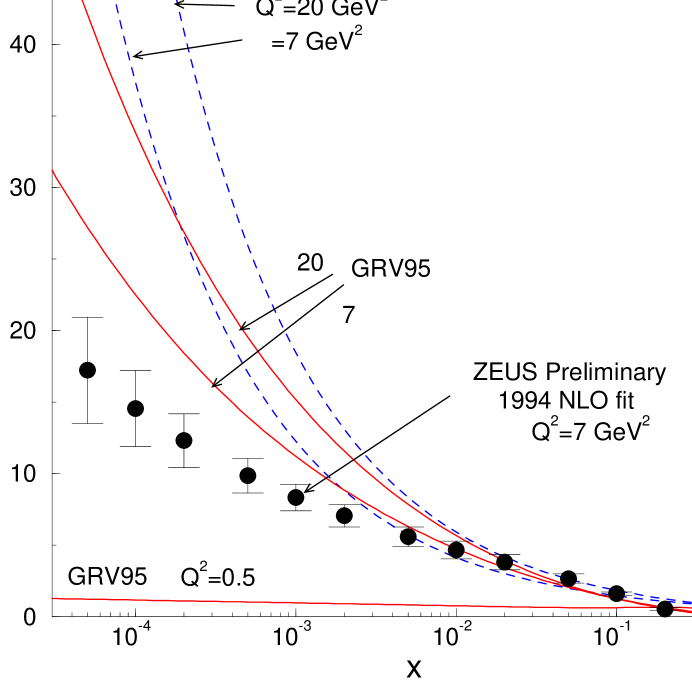
Figure 1: The GRV95 NLO[19] and BFKL-like[5] parametrizations of the gluon structure function, $xG(x,Q^{2})$, for $Q^{2}=7,20$ GeV² are compared to preliminary ZEUS “data”[17] from HERA.

In order to compute $\chi$ we use the GRV95 NLO($\overline{MS}$) parametrization[19] of the nucleon structure functions. Figure 1 shows how the parametrization of the gluon structure compares to preliminary “data” at $Q^{2}=7$ GeV² from HERA[17, 18] obtained via a DGLAP analysis of the scaling violations from $F_{2}(x,Q^{2})$. Also shown is the BFKL-like parametrization of the gluon structure used in [5] for comparison. Both the GRV95 and the BFKL parametrizations significantly overestimate the moderate $Q^{2}$ data of interest here at $x<10^{-3}$. The preliminary $Q^{2}=20$ data from H1[18] (not shown Fig.1) also lie below the GRV95 parametrization. For our purposes, it is only important that the use of GRV95 and the neglect of gluon shadowing should lead to a reasonable upper bound on $\chi$.

As discussed in the previous sections, the classical regime extends up to $k_{\perp}\ \raisebox{2.75pt}{$<$}\raisebox{-2.75pt}{$\sim$}\ Q_{YM}$ where

$$Q_{YM}(A,s)=\surd\chi(A,s,Q^{2}_{YM})\sim\;(1\;{\rm GeV})\;\left(\frac{A}{200}\right)^{1/6}\;\left(\frac{10^{-4}}{x_{\perp}}\right)^{\delta/2}\;\;,$$ (84)

and $\delta\sim 0.2-0.3$. In principle, this must be determined self-consistently given the scale dependence of the glue. In practice, as shown below, $Q_{YM}$ is only weakly dependent of the reference scale if its above $\sim 2$ GeV². The approximate formula for $Q_{YM}$ summarizes the numerical results below.

In Figure 2, $Q_{YM}$ is plotted for $\sqrt{s}=0.2,6.5,100$ ATeV for heavy nuclear beams with $A=200$ as a function of the scale $Q$ with which the GRV95 structure functions are evaluated in (83). The upper solid curves for each energy correspond to (83) with $x_{0}=x_{\perp}$. The lower curves are obtained by increasing the lower cutoff from $x_{\perp}$ to $2x_{\perp}$. The two long dashed curves at the bottom show the contribution of only the valence quarks to $Q_{YM}$ at $\surd s=0.2,100$ ATeV using $x_{0}=x_{\perp}$. The curves show that the hard nuclear glue dominates for finite nuclei at all collider energies. Note also that $Q_{YM}$ is remarkably independent of the reference $Q$ scale because of a compensation of two competing effects. The increase of $xG$ with $Q$ is compensated by its decrease with increasing value of the minimum hard fraction $x_{0}\sim Q/\surd s$ contributing to the classical source.

At RHIC energies, the boundary of the classical regime remains rather low ($\ \raisebox{2.75pt}{$<$}\raisebox{-2.75pt}{$\sim$}\ 500$ MeV) because the relevant $x$ range, $x_{\perp}>0.005$, is not very small. By LHC energies, on the other hand, gluons down to $x_{\perp}\sim 0.0001$ can contribute, and the classical Yang-Mills scale increases to $Q_{YM}\sim 1$ GeV. Note that to double the $Q_{YM}$ scale at a fixed energy would require an increase of $A$ to $2^{6}\times 200$ if shadowing can be ignored. To double the value of $Q_{YM}$ at fixed $A$ requires decreasing $x_{\perp}$ by a factor $2^{-10}\sim 10^{-3}$. Although asymptotically the scale of $Q_{YM}$ becomes arbitrarily large, this asymptotic behaviour is approached slowly. We conclude that at RHIC energies the classical Yang-Mills radiation dynamics is likely to modify mainly the nonlinear, nonperturbative beam jet regime. In that regime the perturbative analysis must certainly be extended into the full nonlinear regime via detailed numerical simulations. By LHC energies it appears that the classical Yang-Mills radiation begins to overlap into the perturbative minijet domain with $k_{\perp}\sim 1$ GeV.

The very small $x$ and very large $A$ limits, where perturbative classical radiation can be computed, provide an novel calculable theoretical limit. It provides qualitatively useful insight at RHIC energies and may be semi-quantitative already at LHC energies. In future studies it will be especially important to extend work with this model into the nonlinear regime to clarify the mechanisms for color screening in $A+A$ reactions at the lower $k_{\perp}\sim\alpha Q_{YM}$ scale. Present estimates for initial conditions in $A+A$ based on mini-jet pQCD analysis[6, 7, 8] vary considerably because of the necessity to introduce a cutoff scale, $p_{0}\sim 1-2$ GeV, to regulate the naive infrared divergent Rutherford rates. That cutoff has thus far been estimated either (1) phenomenologically by imposing observed constraints from extensive $pp,p\bar{p}\rightarrow\pi,K,p,X$ systematics as in [7, 8] or (2) using kinetic theory estimates [20] which are sensitive to formation physics effects. One of the great theoretical advantages of the classical Yang-Mills approach is that the long wavelength nonlinear dynamics involving pre-asymptotic field configurations can be taken into account (at least numerically) without invoking kinetic theory or formation physics assumptions. In the theoretical $\alpha Q_{YM}\gg 1$ GeV domain, that physics may be accessible using perturbative techniques. In the experimentally accessible $\alpha Q_{YM}<1$ GeV regime, numerical solutions of the Yang-Mills equations, as for example in [21], are likely to provide additional insight into that problem. The classical Yang-Mills model[1, 2] is one of the practical tools at present to approach the study of asymptotically high energy reactions, where many unsolved and interesting theoretical problems remain.

Acknowledgements: We are grateful to the Institute of Nuclear Theory and Wick Haxton for supporting the INT-96-3 program where this work was performed. Numerous useful discussions with K. Eskola, X. Guo, Y. Kovchegov, A. Kovner, J. Jalilian-Marian, K. Lee, A. Leonidov, E. Levin, A. Makhlin, A. Mueller, D. Rischke, S. Ritz, R. Venugopalan, and B. Zhang and other participants during that program are also gratefully acknowledged. This work was also supported by the Director, Office of Research, Division of the Office of High Energy and Nuclear Physics of the Department of energy under contracts DOE-FG02-93ER40764 and DOE-FG02-87ER40328.

5 Figure Captions

Figure 1: The GRV95 NLO[19] and BFKL-like[5] parametrizations of the gluon structure function, $xG(x,Q^{2})$, for $Q^{2}=7,20$ GeV² are compared to preliminary ZEUS “data”[17] from HERA.

Figure 2: The classical Yang-Mills scale, $Q_{YM}$, from (83) is shown for $A=200$ nuclei at collider energies $\surd s=0.2,6.5,100$ ATeV as a function of the reference scale, $Q$, used to evaluate the GRV95[19] structure functions. Upper curves and lower curves for each energy correspond to taking the lower cutoff scale $x_{0}=x_{\perp},2x_{\perp}$, respectively. The bottom two dashed curves give the valence quark contributions at $\surd s=0.2,100$ ATeV.

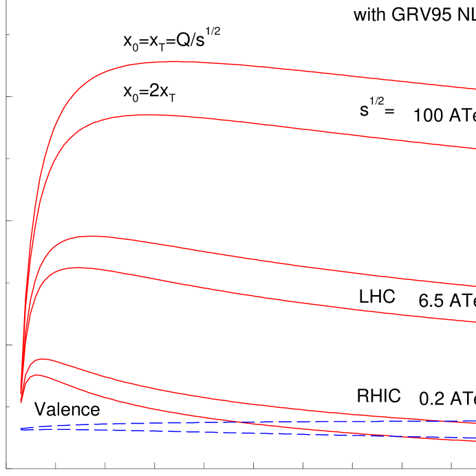
Figure 2: The classical Yang-Mills scale, $Q_{YM}$, from (83) is shown for $A=200$ nuclei at collider energies $\surd s=0.2,6.5,100$ ATeV as a function of the reference scale, $Q$, used to evaluate the GRV95[19] structure functions. Upper curves and lower curves for each energy correspond to taking the lower cutoff scale $x_{0}=x_{\perp},2x_{\perp}$, respectively. The bottom two dashed curves give the valence quark contributions at $\surd s=0.2,100$ ATeV..

References

- [1] Larry McLerran, Raju Venugopalan, Phys.Rev.D49 (94) 2233 ; 3352 ; Phys.Rev. D50 (1994) 2225; Phys.Rev.D53:458-475,1996
- [2] Alex Kovner, L. McLerran, H. Weigert, Phys.Rev.D52 (95) 3809
- [3] J.Gunion and G. Bertsch, PRD 25 (82) 746
- [4] L.V. Gribov, E.M. Levin, M.G. Ryskin , Phys.Lett. 100B (1981) 173; Phys.Lett. 121B (1983) 65; Phys.Rept. 100 (1983) 1; E.M. Levin and M.G. Ryskin, Phys.Rept. 189 (1990) 267.
- [5] K.J. Eskola, A.V. Leonidov, P.V. Ruuskanen, Nucl. Phys. B481 (1996) 704.
- [6] K. Kajantie, P.V. Landshoff, J. Lindfors, Phys. Rev. Lett. 59 (1987) 2527, J.P. Blaizot, A.H. Mueller, Nucl. Phys. B 289 (1987) 847, K.J. Eskola, K. Kajantie, J. Lindfors, Nucl. Phys. B 323 (1989) 37.
- [7] X.N. Wang and M. Gyulassy, Phys. Rev. D 44 (1991) 3501; D 45 (1992) 844, Phys. Rev. Lett. 68 (1992) 1480.
- [8] K. Geiger. BNL-63762, Jan 1997, e-Print Archive: hep-ph/9701226; Phys.Rev.D54:949-988,1996.
- [9] P. Braun-Munzinger, H.J. Specht, R. Stock, and H. Stöcker, eds., Quark Matter ’96, Nucl. Phys. A610 (1996) 1c.
- [10] J. Jalilian-Marian, A. Kovner, L. McLerran, H. Weigert, hep-ph/9606337.
- [11] Yu.V. Kovchegov, PRD54 (1996) 5463.
- [12] Y.V. Kovchegov and D. H. Rischke, CU-TP-824 (1997), e-Print Archive: hep-ph/9704201.
- [13] E.A. Kuraev, L.N. Lipatov, V.S. Fadin, Sov.Phys.JETP 45:199-204,1977; Ya.Ya. Balitskii, L.N. Lipatov Sov.J.Nucl.Phys.28:822-829,1978;
- [14] M. Gyulassy and X.N. Wang, Nucl. Phys. B420 (1994) 583.
- [15] S.K.Wong, Nuovo Cim 65A (1970) 689; U. Heinz, Ann Phys. (N.Y.) 161 (1985) 48; A.V. Selikov and M. Gyulassy, Phys. Lett. B316 (1993) 373.
- [16] V.N. Gribov, L.N. Lipatov, Sov.J.Nucl.Phys.15:675-684,1972; G. Altarelli and G. Parisi, Nucl.Phys.B126:298,1977; Yu. Dokshitzer, Sov.Phys.JETP 46 (1977) 1649.
- [17] S. Ritz private communication; ZEUS preliminary data presented at the DURHAM workshop 1996.
- [18] S. Aid et al., H1 Collab., Nucl. Phys. B470 (1996) 3
- [19] M. Gluck, E. Reya, A. Vogt, Z.Phys.C67 (95) 433
- [20] K.J. Eskola, B. Müller, Xin-Nian Wang, Phys.Lett.B374 (1996) 20.
- [21] T.S. Biro, C. Gong, B. Müller, A. Trayanov, Int. J. Mod. Phys. C5 (1994) 113-149; Phys.Rev.D49 (1994) 607, 5629.