Abstract

Nuclear-polarizability corrections that go beyond unretarded-dipole approximation are calculated analytically for hydrogenic (atomic) S-states. These retardation corrections are evaluated numerically for deuterium and contribute -0.68 kHz, for a total polarization correction of 18.58(7) kHz. Our results are in agreement with one previous numerical calculation, and the retardation corrections completely account for the difference between two previous calculations. The uncertainty in the deuterium polarizability correction is substantially reduced. At the level of 0.01 kHz for deuterium, only three primary nuclear observables contribute: the electric polarizability, $\alpha_{E}$, the paramagnetic susceptibility, $\beta_{M}$, and the third Zemach moment, $\langle r^{3}\rangle_{(2)}$. Cartesian multipole decomposition of the virtual Compton amplitude and its concomitant gauge sum rules are used in the analysis.

Introduction

The remarkable experiments presently being performed in Garching[1] and Paris[2] on the spectroscopy of hydrogen isotopes have astonishing precision. The Rydberg currently has an uncertainty of 9 parts per trillion, while the isotope shift between deuterium and hydrogen 1S - 2S transitions has a reported uncertainty of 3 parts per billion, and this is expected to be lowered soon by an order of magnitude[3].

The isotope-shift measurements afford a unique opportunity for nuclear physics. The traditional technique for determining nuclear sizes is to scatter relativistic electrons from nuclei, determine the charge form factor, and extrapolate this to small momentum transfers, thus determining the mean-square charge radius, $\langle r^{2}\rangle$. It is extremely difficult to perform the latter measurements with an absolute accuracy of one percent or less, and this sets limits on the accuracy of the charge radius. The currently accepted value of the charge radius of the proton[4], $\langle r^{2}\rangle^{1/2}_{p}=0.862(12)$ fm, corresponds to an uncertainty in $\langle r^{2}\rangle$ of nearly 3 percent, and the recently determined deuteron radius[5], $\langle r^{2}\rangle_{d}^{1/2}=2.128(11)$ fm, has an uncertainty in $\langle r^{2}\rangle$ of 1 percent. For the 1S-2S d-p isotope shift[1] the nuclear-size correction contributes approximately -5000 kHz (roughly the same as the QED corrections) out of a total of 670 GHz. The reported[3] uncertainty of 2 kHz corresponds to a precision of better than one part per thousand in $\langle r^{2}\rangle$.

In addition to static size corrections, the electron polarizes the nucleus and produces nuclear-polarizability corrections. In order to use the isotope shift as a precise gauge of nuclear size differences, it is necessary to compute these polarizability corrections as accurately as possible, and that is the goal of this work.

There have been several calculations of these corrections for deuterium [6, 7, 8, 9, 10, 11]. The bulk of the effect ($\approx$19 kHz in toto) is caused by the Coulomb interaction distorting the nucleus ($\approx$17 kHz) with a smaller ($\approx$2 kHz) contribution from the virtual transverse photons. In leading order (unretarded-dipole approximation) the electric polarizability, $\alpha_{E}$, dominates the process and accounts for 19.26(6) kHz in nonrelativistic approximation for the deuteron [11]. This numerical result summarized calculations for a group of “second-generation” potentials, which fit the nucleon-nucleon scattering data well enough to be considered alternative phase-shift analyses of that data.

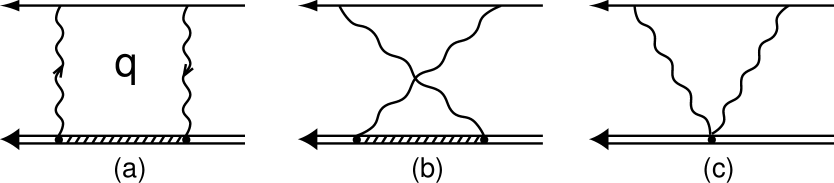
Figure 1: Nuclear polarization corrections with direct (a), crossed (b), and seagull (c) contributions are illustrated. Single lines represent an electron, double lines a nucleus, and shaded double lines depict an excited nucleus, with the seagull vertex maintaining gauge invariance.

There exists a single calculation [7], using first-generation nuclear potentials, that goes beyond the unretarded-dipole approximation and includes retardation, higher multipoles, the effect of the finite sizes of the nucleons, seagulls, and even meson-exchange currents. Results for this calculation are smaller by $\mathrel{\raise 2.0pt\hbox to9.0pt{\raise-7.0pt\hbox{$\sim$}\hss{$>$}}}$ 0.5 kHz than for those using the unretarded-dipole approximation. That calculation was performed by constructing nuclear charge and current (transition) densities and performing a difficult double integral over the momentum and energy transferred across each photon line (see Figure 1). Our goal is to reduce that calculation to an analytic series in various size-dependent nuclear observables, and keep only those that are expected to contribute at a level of greater than 0.01 kHz. The resulting expression is fairly simple and depends only on three primary nuclear observables: the electric polarizability, $\alpha_{E}$, the paramagnetic susceptibility, $\beta_{M}$, and the third Zemach moment [12, 13], $\langle r^{3}\rangle_{(2)}$ , of the charge distribution. Meson-exchange currents[14] play a small role that is easily incorporated in the calculation. Our final result is in excellent agreement with the difficult but comprehensive calculation of Ref. [7]. We will produce a final estimate for the complete polarizability correction of 18.58(7) kHz, based on second-generation potentials. It will be not be easy to improve this result significantly, because it will be difficult to increase the precision of the nuclear observables on which the result depends.

Higher Polarizabilities

The integrals over momentum transfer in the loops that define the generalized polarizability correction are difficult, rather complicated, and extremely tedious. For all these reasons, we have relegated them to Appendix A. The constraints of gauge invariance are crucial to impose (the results are infrared divergent otherwise), but are also tedious to develop, although they have been known for decades[15]. Consequently, a brief presentation of the necessary relations has been relegated to Appendix B. Only those parts of the calculation that we will treat numerically are given directly below. To the order that we work, gauge invariance has been properly implemented.

We first define the electric polarizability[15, 16], $\alpha_{E}$, in terms of the electric-dipole operator, ${\bf D}$,

$$\alpha_{E}=\frac{2\alpha}{3}\sum_{N\neq 0}\frac{|\langle N|{\bf D}|0\rangle|^{2}}{E_{N}-E_{0}}\,,$$

and the logarithmic mean-excitation energy[11, 17], $\bar{E}$, by

$$\log(\bar{E}/m_{e})\,\alpha_{E}=\frac{2\alpha}{3}\sum_{N\neq 0}\frac{|\langle N|{\bf D}|0\rangle|^{2}}{E_{N}-E_{0}}\log\left[(E_{N}-E_{0})/m_{e}\right]\,.$$

Similarly, we define the paramagnetic susceptibility[15, 16], $\beta_{M}$, in terms of the magnetic-(dipole) moment operator, $\mu$, (see Eq. (B8))

$$\beta_{M}=\frac{2\alpha}{3}\sum_{N\neq 0}\frac{|\langle N|\mbox{\boldmath$\mu$}|0\rangle|^{2}}{E_{N}-E_{0}}\,,$$

together with its mean-excitation energy, $\bar{E}$,

$$\log(\bar{E}/m_{e})\,\beta_{M}=\frac{2\alpha}{3}\sum_{N\neq 0}\frac{|\langle N|\mbox{\boldmath$\mu$}|0\rangle|^{2}}{E_{N}-E_{0}}\log\left[(E_{N}-E_{0})/m_{e}\right]\,.$$

A close relative of $\alpha_{E}$ is

$$\Delta\alpha_{E}=\frac{2\alpha}{3}\sum_{N\neq 0}\frac{|\langle N|{\bf D}|0\rangle|^{2}}{(E_{N}-E_{0})^{3}}\,,$$

together with its logarithmic mean-excitation energy analogously defined. Although we have used (and will write below) $\bar{E}$ for each of the different mean-excitation energies for notational simplicity, they are distinct (although similar) numbers. They will always be grouped with the operators that define them. In the formulae above, $\alpha$ is the fine-structure constant, $m_{e}$ is the electron mass, $|N\rangle$ is the Nth nuclear state (the Nth eigenstate of $H_{0}$) with energy, $E_{N}$, and $N=0$ labels the ground state.

The inelastic charge density (squared) can be rewritten in cases where there are no energy factors[18]

$$\sum_{N\neq 0}\langle 0|\rho^{\dagger}({\bf x})|N\rangle\langle N|\rho({\bf y})|0\rangle=\langle 0|\rho^{\dagger}({\bf x})\rho({\bf y})|0\rangle-\rho_{0}(x)\rho_{0}(y)\,,$$

where

$$\rho_{0}(x)=\langle 0|\rho({\bf x})|0\rangle\,,$$

$\rho({\bf x})$ is the nuclear charge (-density) operator and $\int d^{3}x\,\rho_{0}(x)=Z$, the nuclear charge.

With these definitions, we can rewrite Eq. (A30) in the form

$$\Delta E_{n}=-4\alpha\,m_{e}|\phi_{n}(0)|^{2}\left[\frac{5\alpha_{E}}{4}[\log(2\bar{E}/m_{e})+\frac{19}{30}]+\frac{15}{16}m_{e}^{2}\,\Delta\alpha_{E}[\log(2\bar{E}/m_{e})-\frac{283}{300}]\right.$$

$$- \frac{\beta_{M}}{4}[\log(2\bar{E}/m_{e})-\frac{1}{6}]+\frac{\pi\alpha}{12}\int d^{3}x\int d^{3}y\,|{\bf x}-{\bf y}|^{3}\,\left[\langle 0|\rho^{\dagger}({\bf x})\rho({\bf y})|0\rangle-\rho_{0}(x)\rho_{0}(y)\right]$$

$$+ \left.\Delta B\rule{0.0pt}{12.91663pt}\right]\,,\hskip 354.12256pt(8)$$

where

$$\Delta B=\frac{\alpha}{5}\left(\gamma+\log\left(\bar{E}\bar{z}\right)-\frac{39}{20}\right)\int d^{3}x\int d^{3}y\;\langle 0|\Delta B({\bf x},{\bf y})|0\rangle\,,$$

and

$$\Delta B({\bf x},{\bf y})=B^{ii}_{\rm in}({\bf x},{\bf y})[{\bf x}\cdot{\bf y}-y^{2}]+B^{ij}_{\rm in}({\bf x},{\bf y})[-2y^{i}y^{j}+x^{i}y^{j}+y^{i}x^{j}]+\cdots\,.$$

We have dropped a large variety of small terms in $\Delta B$ (indicated by dots and with relative coefficients $\sim$1/10) that arise from the seagull and current terms (converted using gauge sum rules; see Appendix A). Gauge sum rules and approximating $E_{N}-E_{0}$ by $\bar{E}$ and $z\equiv|{\bf x}-{\bf y}|$ by $\bar{z}$ (i.e., constants) were used to obtain Eqs. (9) and (10). The small correction $\Delta B$ arises from the Coulomb interaction; we will also use the alternative expression in Eq. (A31). Note that the term $\sim|{\bf x}-{\bf y}|^{3}$ contributes to all electric multipoles, unlike the others, which are either electric- or magnetic-dipole in nature. Only ground-state properties are needed to construct the former term.

In order to proceed further, we need to specify our nuclear model. The charge operator $\rho({\bf x})$ is given by

$$\rho({\bf x})=\sum_{i=1}^{A}\hat{e}_{i}({\bf x}-{\bf x}_{i})\,,$$

where

$$\hat{e}_{i}=\hat{e}_{p}(i)\;e_{p}({\bf x}-{\bf x}_{i})+\hat{e}_{n}(i)\;e_{n}({\bf x}-{\bf x}_{i})$$

counts protons (with $\hat{e}_{p}$) and neutrons (with $\hat{e}_{n}$) and multiplies each species by its intrinsic charge distribution. The form (11) is nothing more than the usual folding of $\hat{e}_{i}(x)$ with $\delta^{3}({\bf x}-{\bf x}_{i})$. Forming $\int d^{3}x\,{\bf x}\,\rho({\bf x})=\sum_{i}\hat{e}_{p}(i){\bf x}_{i}$ demonstrates that finite size does not modify the electric-dipole operator.

The current operator needed to construct $\mu$ consists of three distinct parts: the spin-magnetization current, the orbital current, and meson-exchange currents (MEC). We ignore nucleon finite size, which does not contribute to this order, and find[19]

$$\mbox{\boldmath$\mu$}=\sum_{i=1}^{A}\left(\frac{\hat{\mu}(i)\,\mbox{\boldmath$\sigma$}(i)+\hat{e}_{p}(i)\,{\bf L}(i)}{2M}\right)+\mbox{\boldmath$\mu$}_{MEC}\,,$$

where the spin-magnetization current is determined by

$$\hat{\mu}(i)=\mu_{p}\,\hat{e}_{p}(i)+\mu_{n}\,\hat{e}_{n}(i)\,.$$

Note that the isoscalar and isovector nucleon magnetic moments are very different in size: $\mu_{s}\equiv\mu_{p}+\mu_{n}=0.8798\ldots$ and $\mu_{v}\equiv\mu_{p}-\mu_{n}=4.7059\ldots$. The large value of the isovector nucleon magnetic moment will play a determinative role. We eschew writing out our model for the two-body pion-exchange currents(i.e., MEC), which is discussed in Ref. [19]. This model has had its pion-nucleon form factor adjusted to reproduce the experimental thermal $n-p$ radiative capture rate [20]. As the contribution of $\beta_{M}$ is relatively small and the MEC a small part of this, the overall MEC contribution is nearly negligible, but has been included for completeness.

Our final ingredient is the Compton seagull operator. This operator is comprised of several components[21]: impulse approximation, plus meson-exchange currents[22], plus …. We expect the meson-exchange currents to be possibly comparable to the impulse approximation, based on sum-rule studies[23]. We will work only with the impulse-approximation component, which has the form[15]

$$B^{ij}({\bf x},{\bf y})=\sum_{i=1}^{A}\hat{e}_{i}({\bf x}-{\bf x}_{i})\;\hat{e}_{i}({\bf y}-{\bf x}_{i})\,.$$

The pion-exchange component of the deuteron’s diamagnetic susceptibility (see Eq. (A29) and Refs. [21, 22]) has been shown to be tiny.

Numerical Calculations

Podolsky’s method[24] is very convenient for calculating $\alpha_{E}$ and $\beta_{M}$. Any generalized polarizability of the type displayed in Eqs. (1) and (3) can be calculated as follows. Equation (1) is fully equivalent to

$$\alpha_{E}=2\alpha\;\langle 0|D_{z}|\Delta\Psi_{z}\rangle\,,$$

where

$$(H_{0}-E_{0})\;|\Delta\Psi_{z}\rangle\;=\;D_{z}|0\rangle$$

is solved subject to finite boundary conditions. One must be careful to exclude the ground state from the sum over N in Eq. (3) for $\beta_{M}$. This necessitates a projection orthogonal to the ground state on the right-hand side of Eq. (17) (with $D_{z}$ replaced by $\mu_{z}$ in both Eqs. (16) and (17)).

For the deuteron, one impulse-approximation calculation of $\beta_{M}$ exists[21] with a value of 0.065 fm³. This is dominated by ${}^{1}\!S_{0}$ intermediate states. Indeed, an upper limit for all triplet intermediate states is $\beta^{t}_{M}\leq 0.0003\,{\rm fm}^{3}$, obtained[21] by replacing the energy denominator in Eq. (3) by its smallest possible value ($E_{d}$, the deuteron binding energy), and then using closure and completing the algebra. Moreover, the ${}^{1}\!D_{2}$-state contribution is tiny, and the ${}^{1}\!S_{0}$ intermediate states dominate completely.

The logarithmic mean-excitation energies are calculated using a trick[25]. We define a quantity closely related to $\alpha_{E}$

$$\alpha_{E}(\xi)=\frac{2\alpha}{3}\;\sum_{N\neq 0}\;\frac{|\langle N|{\bf D}|0\rangle|^{2}}{\xi f+E_{N}-E_{0}}\,,$$

where $f$ is an energy-scaling factor $\sim$ 3-5$E_{d}$ inserted for convenience. An integral over $\xi$ produces a logarithm, and one finds a convenient numerical algorithm for $\bar{E}$ in

$$\alpha_{E}(0)\,\log\;(2\bar{E}/m_{e})=\int^{1}_{0}\;\frac{d\xi}{\xi}[\alpha_{E}(\xi)-\alpha_{E}(0)+\alpha_{E}(1/\xi)]-\alpha_{E}(0)\,\log(m_{e}/2f)\,,$$

where $\bar{E}$ is independent of $f$, and Eq. (19) is fully equivalent to Eq. (2).

The electric polarizability was calculated and thoroughly discussed in Ref. [11]. One found there

$$\hskip 144.54pt\alpha_{E} = 0.6328(17)\,{\rm fm}^{3}$$

$$\log(2\bar{E}/m_{e}) = 2.9620(5)\hskip 173.44756pt(20)$$

$$\nu_{\rm pol}^{\alpha_{E}} = 19.26(6)\,{\rm kHz}=(16.98)+(2.28)\;{\rm kHz}\,,$$

where the latter is broken down into Coulomb, transverse, and total contributions. This calculation did not incorporate relativistic corrections to the deuteron.

Table 1: Impulse-approximation deuteron magnetic susceptibilities, $\beta_{\rm M}$, in units of fm³, logarithmic mean-excitation-energy ratios, $\log(2\bar{E}/m_{e})$, and corresponding deuteron 1S-2S polarization-energy shifts, $\nu_{\rm pol}$, in kHz. The RSC potential labelled [-23] has had its ${}^{1}\!S_{0}$ part modified to produce the correct n-p scattering length.

Potential Model	$\beta_{\rm M}({\rm fm}^{3})$	$\log(2\bar{E}/m_{e})$	$\nu_{\rm pol}({\rm kHz})$
Second-Generation Potentials
Argonne V18	0.0678	2.4724	-0.265
Nijmegen (loc-rel)	0.0677	2.4726	-0.264
Nijmegen (loc-nr)	0.0677	2.4732	-0.264
Nijmegen (nl-rel)	0.0677	2.4726	-0.264
Nijmegen (nl-nr)	0.0676	2.4732	-0.264
Nijmegen (full-rel)	0.0675	2.4728	-0.264
Reid Soft Core (93)	0.0674	2.4744	-0.264
First-Generation Potentials
Bonn (CS)	0.0682	2.4738	-0.267
Argonne V14	0.0674	2.4733	-0.263
Reid Soft Core (68)[-23]	0.0669	2.4748	-0.261
Nijmegen (78)	0.0663	2.4947	-0.261
Super Soft Core (C)	0.0659	2.4982	-0.260
de Tourreil-Rouben-Sprung	0.0656	2.4969	-0.259
Paris	0.0653	2.5008	-0.258
Reid Soft Core (68)	0.0647	2.5031	-0.256

Table 2: Full deuteron magnetic susceptibilities, $\beta_{\rm M}$, in units of fm³, logarithmic mean-excitation-energy ratios, $\log(2\bar{E}/m_{e})$, and corresponding deuteron 1S-2S polarization-energy shifts, $\nu_{\rm pol}$, in kHz. The RSC potential labelled [-23] has had its ${}^{1}\!S_{0}$ part modified to produce the correct n-p scattering length.

Potential Model	$\beta_{\rm M}({\rm fm}^{3})$	$\log(2\bar{E}/m_{e})$	$\nu_{\rm pol}({\rm kHz})$
Second-Generation Potentials
Nijmegen (full-rel)	0.0780	2.5003	-0.308
Nijmegen (nl-rel)	0.0778	2.4981	-0.307
Nijmegen (nl-nr)	0.0777	2.4987	-0.307
Nijmegen (loc-rel)	0.0775	2.4972	-0.306
Nijmegen (loc-nr)	0.0774	2.4978	-0.306
Reid Soft Core (93)	0.0775	2.5005	-0.306
Argonne V18	0.0774	2.4963	-0.305
First-Generation Potentials
Argonne V14	0.0774	2.4996	-0.306
Reid Soft Core (68)[-23]	0.0769	2.5002	-0.304
Bonn (CS)	0.0766	2.4935	-0.302
Nijmegen (78)	0.0751	2.5172	-0.299
de Tourreil-Rouben-Sprung	0.0748	2.5221	-0.298
Super Soft Core (C)	0.0747	2.5218	-0.298
Paris	0.0743	2.5253	-0.297
Reid Soft Core (68)	0.0742	2.5295	-0.297

The analogous calculations for $\beta_{M}$ are listed in Tables I and II for a variety of first- and second-generation potentials[26, 27, 28, 29, 30, 31, 32, 33, 34, 35]. The results of Table I are for the impulse-approximation magnetic moment (no MEC), while those of Table II incorporate MEC, as well. The latter increases the former by approximately 15%, which is quite typical for isovector transitions. We average the various second-generation results and estimate

$$\hskip 144.54pt\beta_{M} = 0.0777(3)\,{\rm fm}^{3}$$

$$\log(2\bar{E}/m_{e}) = 2.498(2)\hskip 177.06128pt(21)$$

$$\nu_{\rm pol}^{\beta} = -0.307(2)(6)\,{\rm kHz}\,.$$

These uncertainties do not include uncertainties in the MEC, which are possibly 1-2% of the total result (this is subjective); the latter is reflected in the second error (6) in the last Eq. (21). This polarization contribution is nonnegligible only because $\mu_{v}=4.7$; a more “normal” size $\sim$1 would reduce the contribution by a factor of $\sim$25. Our $\nu_{\rm pol}$ is in reasonable agreement with the zero-range result of Ref. [9].

The very small corrections, $\Delta\alpha_{E}$, can be accurately estimated in zero-range approximation (which we used as a tool in Ref. [11]). We first calculate $\alpha^{0}_{E}(\xi)$ using Eq. (18) and find

$$\alpha^{0}_{E}(\xi)=\frac{\alpha\,\mu A^{2}_{s}}{12\kappa^{3}}\frac{(\kappa^{2}+\bar{\kappa}^{2}+4\kappa\bar{\kappa})}{(\kappa+\bar{\kappa})^{4}}\,,$$

where the asymptotic (reduced) s-state wave function of the deuteron has the form: $A_{s}\,e^{-\kappa r}$. Moreover, $\bar{\kappa}^{2}\equiv\kappa^{2}(1+\xi f)$, and $\mu$ is the n-p reduced mass. Performing two derivatives leads to

$$m^{2}_{e}\,\Delta\alpha^{0}_{E}=\frac{7\alpha^{0}_{E}\,m^{2}_{e}}{24E^{2}_{d}}=0.0098\;{\rm fm}^{3}\,,$$

and is accurate to better than 1/2%. The following integral (similar to Eq. (19)) produces the logarithmic mean-excitation energy

$$\hskip 18.06749pt\log\;(2\bar{E}/m_{e}) = \frac{1}{f^{2}\Delta\alpha^{0}_{E}}\left[\int^{1}_{0}\;\frac{d\xi}{\xi^{3}}[\alpha^{0}_{E}(\xi)-\alpha^{0}_{E}(0)-\xi\alpha_{E}^{0\,\prime}(0)-\frac{\xi^{2}}{2}\alpha_{E}^{0\,\prime\prime}(0)]\right.$$

$$+ \left.\int^{1}_{0}\;d\xi[\xi\alpha^{0}_{E}(1/\xi)-\xi\alpha^{0}_{E}(0)-\alpha_{E}^{0\,\prime}(0)]\rule{0.0pt}{15.0694pt}\right]\,-\log(m_{e}/2f)$$

$$= 2.648\,.\hskip 271.0125pt(24)$$

These results produce a total correction from $\Delta\alpha_{E}$:

$$\nu^{\Delta\alpha_{E}}_{\rm pol}=0.106\,{\rm kHz}\;=(0.060)+(0.046)\,{\rm kHz}\,,$$

which has been broken down into Coulomb and transverse parts, respectively.

The remaining large quantity in Eq. (8) is the retardation correction proportional to $\rho_{\rm in}({\bf x},{\bf y})$. Using Eq. (11), we expand that result and find

$$\rho^{\dagger}({\bf x})\rho({\bf y})=\sum_{i\neq j}\hat{e}_{i}({\bf x}-{\bf x}_{i})\hat{e}_{j}({\bf y}-{\bf x}_{j})+\sum_{i}\hat{e}_{p}(i)e_{p}({\bf x}-{\bf x}_{i})e_{p}({\bf y}-{\bf x}_{i})+\hat{e}_{n}(i)e_{n}({\bf x}-{\bf x}_{i})e_{n}({\bf y}-{\bf x}_{i})\,.$$

Note that if the neutron’s charge distribution is set to zero, the first term vanishes for the deuteron (one nucleon must be a neutron), and only the second term survives. Shifting the ${\bf x}$ and ${\bf y}$ integrals each by ${\bf x}_{i}$ in that case produces $\langle r^{3}\rangle^{p}_{(2)}$, while the $\rho_{0}(x)\rho_{0}(y)$ term generates $\langle r^{3}\rangle^{d}_{(2)}$, and a retardation correction

$$\frac{\pi\alpha}{12}\left[-\langle r^{3}\rangle^{d}_{(2)}+\langle r^{3}\rangle^{p}_{(2)}\right]\equiv\frac{\pi\alpha}{12}\Delta\langle r^{3}\rangle_{(2)}\,,$$

where

$$\langle r^{n}\rangle_{(2)}=\int d^{3}r\,r^{n}\,\rho_{(2)}(r)\,,$$

and

$$\rho_{(2)}(r)=\int d^{3}z\,\rho(|{\bf z}-{\bf r}|)\,\rho(z)\equiv\rho\otimes\rho$$

is the convoluted (Zemach[12, 13]) density. In Eq. (27), the first of the third moments is calculated with respect to the total deuteron (including the finite size of the proton) convoluted charge density and the second with the proton’s convoluted density, $\rho_{p}$. In what follows below we will specialize to the deuteron, and denote by $\rho_{d}$ the deuteron’s ground-state charge density (called $\rho_{0}$ before).

For completeness, we include the neutron contributions as well. There will be a two-body correlation term (first term in Eq. (26)) involving $\rho_{n}\otimes\rho_{p}\otimes\bar{\rho}_{d}$, where $\bar{\rho}_{d}$ is slightly modified to account for the vector ${\bf r}$ specifying a correlation, while ${\bf r}/2$ determines the charge density, $\rho_{d}$. In addition to this term, the folded proton density in Eq. (27) is replaced by $(\rho_{p}\otimes\rho_{p}+\rho_{n}\otimes\rho_{n})$ and the deuteron charge density is defined by $(\rho_{p}+\rho_{n})\otimes\rho^{0}_{d}$, where $\rho^{0}_{d}$ is determined by the deuteron wave function alone.

We use a simplified model of the neutron and proton form factors. The proton form factor is taken to have a dipole form with the correct radius[4] (0.862 fm). The neutron form factor is that dipole times $q^{2}$, adjusted overall to match the experimental charge radius of -0.338 fm[36].

Calculations of the various moments are performed by first calculating the deuteron density and then generating a spline fit of it. Then folding is performed and that convoluted density is similarly fit. Moments are calculated ultimately with respect to the final fitted density.

Table 3: Zemach-moment contribution $\Delta\langle r^{3}\rangle_{(2)}$, to the Coulomb-induced retardation correction in units of fm³, and corresponding deuteron 1S-2S polarization-energy shifts, $\nu_{\rm pol}$, in kHz.

Potential Model	$\Delta\langle r^{3}\rangle_{(2)}\,({\rm fm}^{3})$	$\nu_{\rm pol}({\rm kHz})$
Second-Generation Potentials
Argonne V18	-37.45	-0.485
Reid Soft Core (93)	-37.44	-0.484
Nijmegen (loc-nr)	-37.38	-0.484
Nijmegen (loc-rel)	-37.34	-0.483
Nijmegen (nl-rel)	-37.36	-0.483
Nijmegen (nl-nr)	-37.31	-0.483
Nijmegen (full-rel)	-37.20	-0.481
First-Generation Potentials
Super Soft Core (C)	-38.45	-0.498
Nijmegen (78)	-38.27	-0.495
Argonne V14	-38.01	-0.492
de Tourreil-Rouben-Sprung	-37.70	-0.488
Paris	-37.55	-0.486
Bonn (CS)	-37.44	-0.484
Reid Soft Core (68)	-36.87	-0.477

The results for various models (including the effect of neutrons) are listed in Table 3. The neutrons lower the result by approximately 1%. The second-generation results for this retardation (and higher-multipole) correction can be summarized by

$$\Delta\langle r^{3}\rangle_{(2)}=-37.32(12)\;{\rm fm}^{3}\,,$$

and

$$\nu_{\rm pol}^{\rm ret}=-0.483(2)\,{\rm kHz}\,.$$

This process is the only one that we will consider where higher multipoles, retarded $E1$, and nucleon finite size contribute.

The final task will be to estimate the size of $\Delta B$. The “natural” size of terms with numerical coefficients $\sim$1 is $\Delta B\sim\frac{\alpha\langle r^{2}\rangle_{d}}{M}$, while the coefficient $4m_{e}\alpha^{2}|\phi_{n}(0)|^{2}$ has a value 0.05 kHz/fm³. Since $\frac{\langle r^{2}\rangle_{d}}{M}\sim 0.8\,{\rm fm}^{3}$, the natural size is 0.04 kHz. We use $\bar{E}\mathrel{\raise 2.0pt\hbox to9.0pt{\raise-7.0pt\hbox{$\sim$}\hss{$>$}}}$ 10 MeV, $\bar{z}\mathrel{\raise 2.0pt\hbox to9.0pt{\raise-7.0pt\hbox{$\sim$}\hss{$>$}}}$ 4 fm to estimate logarithms and Eqs. (15) and (B12) for the seagull operator. The seagull contribution has a size $\sim\frac{6}{48}$ (0.04 kHz) $\sim$ 0.005 kHz. The higher-order current terms are of similar size, but largely cancel, leaving a very tiny residue. The higher-order charge terms are dominated by quadrupole excitations and have a nominal size $\sim\frac{4}{4}$ (0.04 kHz) $\sim$ 0.04 kHz, which is almost as large as the $\Delta\alpha_{E}$ Coulomb term. It can be shown, however, that this size is an artifact, caused by neglecting some recoil terms. We must perform the estimate more carefully.

If one uses instead the representation in Eq. (A31) for the $z^{4}$ charge terms, and evaluates the double commutators, one finds that the kinetic-energy part of $H_{0}$ vanishes in the point-nucleon limit, and otherwise has a rough size $\sim$ 0.006 kHz. One can also evaluate the potential part of the commutator and find $\sim$ 0.003 kHz. These corrections are not only small, but the comparable sizes of kinetic and potential terms are in accordance with expectations.

Results and Conclusions

Table 4: Contributions in kHz to the deuteron-polarizability frequency shift for the 1S-2S transition together with their respective origins, separated into Coulomb and transverse, and electric dipole, magnetic dipole, and higher-multipole and retardation terms.

Origin	$\alpha_{E}$	$\Delta\alpha_{E}$	$\beta_{M}$	$\Delta\langle r^{3}\rangle_{(2)}$	$\Delta B$	Total
Coulomb	16.98	0.06	-	-0.48	$<$ 0.01	16.56
Transverse	2.28	0.05	-0.31	-	$<$ 0.01	2.02
Total	19.26	0.11	-0.31	-0.48	$\mathrel{\raise 3.0pt\hbox to8.0pt{\raise-6.0pt\hbox{$\sim$}\hss{$<$}}}$ 0.01	18.58

Our final results are tabulated in Table 4, with breakdowns according to their origin. The total for the 1S-2S transition in deuterium is

$$\nu_{\rm pol}=18.58(7)\,{\rm kHz}\,.$$

This is 0.68 kHz less than the leading-order $(\alpha_{E})$ result, and is consistent with the differences between the results of Refs. [7] and [8]. The complete numerical results of Ref. [7] for four first-generation potentials (Paris[31], $AV_{14}$[33], Nijmegen[34],and Bonn CS[30]) are in agreement with our results within 0.02 kHz for Coulomb and transverse parts, which must be regarded as virtually perfect agreement. We note that substantially improving the uncertainty in Eq. (32) will be difficult, because it would entail substantial improvements[11, 37] in the nuclear parameter, $A_{s}$.

A wide variety of physical mechanisms contribute to the final result. Unretarded $E1$ photons (both longitudinal and transverse) generate the electric polarizability. The paramagnetic susceptibility generates a nonnegligible term only because the nucleon isovector magnetic moment is nearly 5. This term is thus $\sim$25 times larger than if it were of “normal” size. A retardation correction contributing to all electric multipoles is moderately important, and is the only one of our terms to which the nucleon form factors contribute. Finally, higher-order terms, including the seagull contribution, are estimated and shown to be tiny.

Acknowledgements

The work of J. L. Friar was performed under the auspices of the United States Department of Energy, while that of G. L. Payne was supported in part by the United States Department of Energy. We would like to thank Winfried Leidemann, Don Sprung, and Joan Martorell for their generous help in providing information about their calculations.

Appendix A

We wish to evaluate the contributions of Figures (1a)-(1c) to the energy of the nth hydrogenic S-state. Because this calculation has been set up before[7], we sketch that part of the derivation.

The nuclear energy and momentum scales are much greater than those of an atom. Consequently, such large momenta flow through the photon and electron propagators in Fig. (1) that only the shortest-range part of the electron wave functions, $|\phi_{n}(0)|^{2}$, contributes to leading order in $Z\alpha$, the product of the nuclear charge, $Z$, and the fine-structure constant, $\alpha$. Consequently, the momentum in both photon propagators is taken to be $q$ (differences in these momenta lead to higher-order terms in $Z\alpha$). It is important to enforce the constraints of gauge invariance[15] on the nuclear part of the interaction (the virtual Compton amplitude), and this is most conveniently handled using Coulomb gauge, which isolates the nuclear charge density from the transverse parts of the currents (Figs. (1a) and (1b)) and seagull (Fig. (1c)). The calculation requires a relativistic treatment of the electron (since $q\gg m_{e}$, the electron mass), but a nonrelativistic (i.e., leading-order) treatment of the nucleus suffices. We expand the nuclear current, $J^{\mu}$, in powers of $1/M$, the nucleon mass, and keep no powers higher than linear. One immediate consequence of the latter is the lack of (nuclear) momentum dependence in the nuclear charge density, $\rho({\bf x})$ (unlike the current density, ${\bf J}({\bf x})$), and the nuclear seagull density[15], $B^{mn}({\bf x},{\bf y})$, which also lacks charge components (i.e., $B^{\mu\nu}=0$ for $\mu=0$ or $\nu=0$). Our conventions follow Ref. [38], and correspond to natural units $(\hbar=c=1)$. We will incorporate meson-exchange currents where required by gauge invariance, although their numerical contribution is ultimately small (see main body of paper). We ignore nuclear recoil corrections ($\sim 1/M_{t}$, the total nucleus mass) in the nuclear operators, but maintain them in reduced-mass factors in the atomic basis states.

The energy shift of the nth hydrogenic S-state due to nuclear polarization is most conveniently calculated by performing the contour integral over the time component of $q^{\mu}(q_{0})$ in the loops of Fig. (1), which leads to[7]

$$\hskip 18.06749pt\Delta E_{pol} = \frac{-2\alpha^{2}m_{e}}{\pi}|\phi_{n}(0)|^{2}\int d^{3}q\left[\sum_{N\neq 0}\left[\frac{(2E+\omega_{N})|\langle N|\rho({\bf q})|0\rangle|^{2}}{Eq^{4}[(E+\omega_{N})^{2}-m^{2}_{e}]}\right.\right.$$

$$+ \left.\left(\left[\frac{q^{2}}{4m^{2}_{e}}\right]\frac{2E+\omega_{N}}{Eq^{4}[(E+\omega_{N})^{2}-m^{2}_{e}]}-\frac{(2q+\omega_{N})}{4m^{2}_{e}q^{3}(q+\omega_{N})^{2}}\right)|\langle N|{\bf J}_{\bot}({\bf q})|0\rangle|^{2}\right]$$

$$+ \left.\frac{B^{ii\bot}_{\rm in}({\bf q})}{8q^{2}m^{2}_{e}}\left(\frac{1}{q}-\frac{1}{E}\right)\right],\hskip 224.03743pt(A1)$$

where $q^{2}\equiv{\bf q}^{2},E=\sqrt{q^{2}+m^{2}_{e}}$, $\omega_{N}=E_{N}-E_{0}$, the energy of excitation (relative to the ground state) of the Nth nuclear state (which by assumption cannot be the ground state). In addition

$$\hskip 130.08621pt\rho({\bf q}) = \int d^{3}x\,e^{i{\bf q}\cdot{\bf x}}\rho({\bf x})\,,\hskip 144.54pt(A2)$$

$$\hskip 130.08621pt{\bf J}({\bf q}) = \int d^{3}x\,e^{i{\bf q}\cdot{\bf x}}{\bf J}({\bf x})\,,\hskip 144.54pt(A3)$$

$$\hskip 72.26999ptB^{ij}_{\rm in}({\bf q}) = \int d^{3}x\int d^{3}y\,e^{i{\bf q}\cdot({\bf x}-{\bf y})}B^{ij}_{\rm in}({\bf x},{\bf y})\,,\hskip 72.26999pt(A4)$$

and “$\bot$” signifies contraction with respect to $\delta^{ij}-\hat{q}^{i}\hat{q}^{j}$ (i.e., ${\bf J}^{2}_{\bot}\equiv J^{i}J^{j}(\delta^{ij}-\hat{q}^{i}\hat{q}^{j})$). Gauge invariance of this nuclear Compton amplitude (discussed in Appendix B) restricts $B^{ij}$ to the “inelastic” part, $B^{ij}_{\rm in}$ (see Eq. (B12)).

Because nuclear momentum, size, and energy scales are given by $Q\sim 1/R\sim$ 100 MeV, $\omega_{N}\sim Q^{2}/2M\sim$ 5 MeV, while $m_{e}\sim$ 0.5 MeV, there are two small dimensionless expansion parameters: $\delta\sim\omega_{N}R\sim 1/20$ and $\beta\sim m_{e}R\sim 1/200$. Consequently, we work in configuration space, where expansions in R are easiest, using techniques introduced in electromagnetically-induced heavy-ion reactions[18]. Similar techniques were used in Refs. [6, 8]. We introduce the inelastic transition densities (squared)

$$\hskip 108.405pt\rho_{\rm in}({\bf x},{\bf y}) = \langle 0|\rho^{\dagger}({\bf x})|N\rangle\langle N|\rho({\bf y})|0\rangle\,,\hskip 108.405pt(A5)$$

$$\hskip 90.3375ptJ^{ij}_{\rm in}({\bf x},{\bf y}) = \langle 0|J^{i\dagger}({\bf x})|N\rangle\langle N|J^{j}({\bf y})|0\rangle\,,\hskip 99.00954pt(A6)$$

and $B^{ij}_{\rm in}({\bf x},{\bf y})$ has already been used in Eq. (A4). We are not interested in hyperfine structure and, consequently, the spin average over nuclear ground-state ($|0\rangle$) azimuthal quantum numbers is assumed, while the sum over these quantum numbers for the intermediate states $(|N\rangle)$ is implicit in Eq. (A1). Consequently, $\rho_{\rm in}$ and $J^{ii}_{\rm in}$ are space scalars. The plane waves in Eqs. (A2 - A4) can then be extracted, appropriate spherical averages over $\hat{{\bf q}}$ performed (e.g., $e^{i{\bf q}\cdot({\bf x}-{\bf y})}\rightarrow\sin(qz)/(qz)$, where ${\bf z}\equiv{\bf x}-{\bf y}$), and the $q$-integrals in Eq. (A1) finally evaluated. This produces the generic result

$$\hskip 72.26999pt\Delta E_{pol} = -8\alpha^{2}m_{e}|\phi_{n}(0)|^{2}\int d^{3}x\int d^{3}y\left[\sum_{N\neq 0}\left[\rho_{\rm in}({\bf x},{\bf y})I_{N}(z)\rule{0.0pt}{10.76385pt}\right.\right.$$

$$+ \left.J^{ii}_{\rm in}({\bf x},{\bf y})J_{N}(z)+J^{ij}_{\rm in}({\bf x},{\bf y})z^{i}z^{j}\bar{J}_{N}(z)\right]$$

$$+ \left.\frac{1}{2}B^{ii}_{\rm in}({\bf x},{\bf y})K(z)+\frac{1}{2}B^{ij}_{\rm in}({\bf x},{\bf y})z^{i}z^{j}\bar{K}(z)\rule{0.0pt}{17.22217pt}\right]\,,\hskip 68.65627pt(A7)$$

where all of our effort will be devoted to obtaining the polarization structure functions: $I_{N}(z),J_{N}(z),\bar{J}_{N}(z),K(z)$, and $\bar{K}(z)$. We will develop general forms and then perform expansions in $(\omega_{N}z)$ and $(m_{e}z)$.

We begin with the charge-charge interaction term, $I_{N}$, which is the most complicated to obtain. All other integrals can be obtained from this one:

$$\hskip 72.26999ptI_{N}(z) = \frac{1}{\omega_{N}z}\int^{\infty}_{0}\frac{dq\,[(2E+\omega_{N})\omega_{N}]\,\sin(qz)}{q^{3}E[(E+\omega_{N})^{2}-m_{e}^{2}]}$$

$$= \frac{1}{\omega_{N}z}\int^{\infty}_{0}\frac{dq\,\sin(qz)}{q^{3}E}\left[1-\frac{q^{2}}{(\omega_{N}+E)^{2}-m_{e}^{2}}\right]$$

$$\equiv \frac{(I^{(0)}(z)-I^{(1)}(z))}{\omega_{N}z}\,.\hskip 184.28871pt(A8)$$

Nominally infrared divergent, that part of $I^{0}(z)$ does not contribute after the integrals over ${\bf x}$ and ${\bf y}$ are performed in Eq. (A7) (the nucleus is assumed to be virtually excited). Ignoring all of these (ultimately vanishing) terms here and in subsequent integrals, we find with $\beta\equiv m_{e}z$

$$\hskip 79.49744ptI^{(0)}(z) = \int^{\infty}_{0}\frac{dq\sin(qz)}{q^{3}E}$$

$$= -\frac{1}{m_{e}^{3}}\int^{\beta}_{0}dx\int^{x}_{0}dy\int^{y}_{0}d\beta^{\prime}\;K_{0}(\beta^{\prime})$$

$$= -\frac{1}{2m_{e}^{3}}\int^{\beta}_{0}d\beta^{\prime}(\beta-\beta^{\prime})^{2}\;K_{0}(\beta^{\prime})\,,\hskip 104.79128pt(A9)$$

where $K_{0}(x)$ is the modified Bessel function of order zero. The function $I^{(0)}(z)$ can easily be expressed in terms of the $Ki_{n}(z)$, the (nth) repeated integrals of $K_{0}(x)$ [see Eqs. (9.6.25) and (11.2.8) of Ref. [39]]. The remaining integral $I^{(1)}$ is more challenging and requires several steps. We define $\xi=\omega_{N}+m_{e}$ and $\xi^{\prime}=\omega_{N}-m_{e}$, assuming $\xi^{\prime}>m_{e}$ for the results reported below (this is easily relaxed), and write

$$\hskip 86.72377ptI^{(1)} = \frac{1}{2m_{e}}\int^{\infty}_{0}\frac{dq}{q}\sin(qz)\left[\frac{-1}{E(E+\xi)}+\frac{1}{E(E+\xi^{\prime})}\right]$$

$$\equiv \frac{\tilde{I}\,^{(1)}(\xi^{\prime};z)-\tilde{I}\,^{(1)}(\xi;z)}{2m_{e}}\,.\hskip 151.76744pt(A10)$$

Using the field-theory trick[40]

$$\frac{1}{E_{1}E_{2}(E_{1}+E_{2})}=\frac{2}{\pi}\int^{\infty}_{0}\frac{d\lambda}{(\lambda^{2}+E^{2}_{1})(\lambda^{2}+E^{2}_{2})}\,,$$

and Eq. (3.737.3) of Ref. [41] the Fourier transforms can be evaluated in the form

$$\hskip 72.26999pt\tilde{I}\,^{(1)}(\xi;z) = \xi\int^{\infty}_{0}\frac{d\lambda}{(\lambda^{2}+\xi^{2})}\frac{(1-e^{-z\sqrt{\lambda^{2}+m^{2}_{e}}}\,)}{(\lambda^{2}+m^{2}_{e})}$$

$$= \frac{\pi}{2m_{e}(\xi+m_{e})}-\frac{\xi}{m_{e}(\xi^{2}-m^{2}_{e})}\left[\int^{\infty}_{1}\frac{dx\,e^{-\beta x}}{x\sqrt{x^{2}-1}}\right.$$

$$- \left.\int^{\infty}_{1}\frac{dx\,x\,e^{-\beta x}}{(x^{2}+\mu^{2})\sqrt{x^{2}-1}}\right],\hskip 130.08621pt(A12)$$

after using partial fractions and $z^{2}\lambda^{2}\equiv\beta^{2}(x^{2}-1)$, and defining $\mu^{2}=\xi^{2}/m^{2}_{e}-1(>0)$. The first of the remaining integrals is $Ki_{1}(\beta)=\pi/2-\int^{\beta}_{0}d\beta^{\prime}K_{0}(\beta^{\prime})$ (use $x=\cosh(t)$ in Eq. (11.2.10) of Ref. [39]). The remaining integral (defined to be $\tilde{I}(\beta;\mu)$ with the minus sign) yields to a further trick; it is the solution of the differential equation

$$\frac{\partial^{2}\tilde{I}(\beta)}{\partial\beta^{2}}+\mu^{2}\tilde{I}(\beta)=K^{\prime}_{0}(\beta)\,,$$

subject to the boundary condition, $\tilde{I}(\infty)\rightarrow 0$ exponentially, for which standard solutions exist:

$$\hskip 14.45377pt\tilde{I}(\beta;\mu) = -\frac{1}{\mu}\int^{\infty}_{\beta}d\beta^{\prime}K^{\prime}_{0}(\beta^{\prime})[\cos(\mu\beta^{\prime})\sin(\mu\beta)-\cos(\mu\beta)\sin(\mu\beta^{\prime})]$$

$$= \frac{-m_{e}}{\xi}\;[\sin(\mu\beta)\log(\mu+\sqrt{\mu^{2}+1})+\frac{\pi}{2}\cos(\mu\beta)]$$

$$+ \int^{\beta}_{0}d\beta^{\prime}K_{0}(\beta^{\prime})[\sin(\mu\beta)\sin(\mu\beta^{\prime})+\cos(\mu\beta)\cos(\mu\beta^{\prime})]\,,\hskip 61.42993pt(A14)$$

after integration by parts and rearrangement. Combining terms from Eq. (A12) and using the last form of Eq. (A9), we obtain $\tilde{I}^{(1)}=-\xi I^{(0)}+\bar{I}(\xi;\beta)$, where

$$\hskip 7.22743pt\bar{I}(\xi;\beta) = \frac{\xi}{m_{e}(\xi^{2}-m^{2}_{e})}\left\{-\frac{\pi m_{e}}{2\xi}(1-\cos(\mu\beta))+\frac{m_{e}}{\xi}\sin(\mu\beta)\log\left[\frac{\xi+\sqrt{\xi^{2}-m_{e}^{2}}}{m_{e}}\right]\right.$$

$$- \int^{\beta}_{0}d\beta^{\prime}K_{0}(\beta^{\prime})\left[\sin(\mu\beta)\sin(\mu\beta^{\prime})+\cos(\mu\beta)\cos(\mu\beta^{\prime})\rule{0.0pt}{15.0694pt}\right.$$

$$- \left.\left.1-\mu^{2}\beta\beta^{\prime}+\frac{\mu^{2}}{2}(\beta^{2}+{\beta^{\prime}}^{2})\right]\right\}\,.\hskip 180.67499pt(A15)$$

Finally, a relatively simple result is obtained

$$\hskip 7.22743ptI_{N}(z) = \frac{1}{2m_{e}\omega_{N}z}\left[\bar{I}(\xi;\beta)-\bar{I}(\xi^{\prime};\beta)\right]$$

$$\cong \frac{-z^{2}}{6\omega_{N}}\left(1+\log\left(\frac{2\omega_{N}}{m_{e}}\right)+\Delta L_{1}\right)+\frac{\pi z^{3}}{24}$$

$$+ \frac{\omega_{N}z^{4}}{40}\left(\frac{}{}\gamma+\log(\omega_{N}z)+\frac{\Delta L_{3}}{3}\;-\frac{39}{20}\right)+O(z^{5})\,,\hskip 97.56493pt(A16)$$

where $\gamma$ is Euler’s constant and

$$\hskip 7.22743pt\Delta L_{n} = \frac{\omega_{N}}{2m_{e}}\left[\left(\frac{\xi^{2}-m_{e}^{2}}{\omega_{N}^{2}}\right)^{n/2}\log\left(\frac{\xi+\sqrt{\xi^{2}-m_{e}^{2}}}{m_{e}}\right)\right.\hskip 122.85876pt(A17)$$

$$- \left.\left(\frac{\xi^{\prime 2}-m_{e}^{2}}{\omega_{N}^{2}}\right)^{n/2}\log\left(\frac{\xi^{\prime}+\sqrt{\xi^{\prime 2}-m_{e}^{2}}}{m_{e}}\right)\right]-\left(1+n\,\log\left(\frac{2\omega_{N}}{m_{e}}\right)\right)$$

$$\cong \frac{m_{e}^{2}}{\omega_{N}^{2}}\left[a_{n}\log\left(\frac{2\omega_{N}}{m_{e}}\right)+b_{n}\right]+\frac{m_{e}^{4}}{\omega_{N}^{4}}\left[\bar{a}_{n}\log\left(\frac{2\omega_{N}}{m_{e}}\right)+\bar{b}_{n}\right]+O\left(m_{e}^{6}/\omega_{N}^{6}\right)\,.$$

Useful values are $(a_{1}=1/2,b_{1}=-5/12)$, $(\bar{a}_{1}=7/8,\bar{b}_{1}=-\frac{449}{480})$, and $(a_{3}=-\frac{1}{2},b_{3}=\frac{1}{12})$. This completes treatment of the charge term.

The current and seagull terms require special treatment because of the transverse projection (i.e., the “$\perp$”). The appropriate current-current terms have the generic form

$$\hskip 18.06749pt\int d^{3}q\,f(q)|\langle N|{\bf J}_{\perp}({\bf q})|0\rangle|^{2} = \int d^{3}x\int d^{3}y\,J^{ij}_{\rm in}({\bf x},{\bf y})\int d^{3}q\,f(q)\left(\delta^{ij}-\frac{q^{i}q^{j}}{q^{2}}\right)e^{i{\bf q}\cdot{\bf z}}$$

$$= \int d^{3}x\int d^{3}y\rule{0.0pt}{17.22217pt}\left\{J^{ii}_{\rm in}({\bf x},{\bf y})\int d^{3}q\,e^{i{\bf q}\cdot{\bf z}}f(q)\right.$$

$$+ \left.J^{ij}_{\rm in}({\bf x},{\bf y})\;\nabla^{i}_{z}\nabla^{j}_{z}\int\frac{d^{3}q\,e}{q^{2}}^{i{\bf q}\cdot{\bf z}}f(q)\right\}.\hskip 57.81621pt(A18)$$

The second q-integral (defined to be $J_{CG}$) can be seen from Eq. (1) to be
$\frac{1}{4m_{e}^{2}}\left[I_{N}(z)-\lim_{m_{e}\rightarrow 0}I_{N}(z)\right]$, while the first integral (defined to be $J^{0}$) is given by [$-\frac{1}{4m_{e}^{2}z}\frac{d^{2}}{dz^{2}}z\left[I_{N}(z)-\lim_{m_{e}\rightarrow 0}I_{N}(z)\right]$]. Both forms have an infrared divergence (which will ultimately disappear because of gauge invariance) and we write $m_{e}\rightarrow 2\lambda$ in divergent logarithms, where $\lambda$ is the equivalent small-$q$ cutoff in the integrals. It is easy to perform the derivatives, take the limits, and perform the subtractions. For the sake of brevity, we quote only the power-series forms.

$$J^{0}\cong\frac{1}{4m_{e}^{2}\,\omega_{N}}\left[\log(2\lambda/m_{e})+\Delta L_{1}-\frac{\omega^{2}_{N}z^{2}}{6}\Delta L_{3}\right]+O(z^{3})\,,$$

$$J_{CG}\cong-\frac{z^{2}}{24m^{2}_{e}\,\omega_{N}}\left[\log(2\lambda/m_{e})+\Delta L_{1}-\frac{\omega_{N}^{2}z^{2}\Delta L_{3}}{20}\right]+O(z^{5})\,.$$

Performing the derivatives in Eq. (A18), and matching to Eq. (A7), we find

$$J_{N}\cong\frac{1}{6m_{e}^{2}\,\omega_{N}}\left[\log(2\lambda/m_{e})+\Delta L_{1}-\frac{\omega_{N}^{2}z^{2}}{5}\Delta L_{3}\right]$$

and

$$\bar{J}_{N}\cong\frac{\omega_{N}\Delta L_{3}}{60m_{e}^{2}}\,.$$

The seagull integrals are straightforward variants of Eq. (A9). We find

$$K\cong-\frac{\log(2\lambda/m_{e})}{6m_{e}^{2}}+\frac{z^{2}}{60}(\gamma+\log(\beta/2)-77/60)+O(z^{4})\,,$$

and

$$\bar{K}\cong-\frac{1}{120}(\gamma+\log(\beta/2)-31/30)+O(z^{2})\,.$$

We have kept terms $\sim R^{4}$ with the charge densities, since the term of $O(1)$ leads to a vanishing result and therefore the leading order $\sim R^{2}$. The currents themselves are of leading order $R^{2}$, so we have kept terms through $R^{4}$ (i.e., of relative order $R^{2}$), as in the charge-density case.

With hindsight, we can identify the dominant terms in the expansion, which are thoroughly discussed in the main text. We note the appearance of $\log(z)$ terms and a $z^{3}$ term. If the Fourier transforms of $\rho$ and $J$ could be term-by-term expanded in $q^{2}$, these terms would be absent. The integrals diverge at some order, signaling this with “non-analytic” terms in $z^{2}\,(e.g.,z^{3}=(z^{2})^{3/2})$. Such terms play an important role in modern effective field theories[42]. In small terms that we will only estimate, $z^{4}$ charge terms and $z^{2}$ seagull terms, we will replace $\log(z)$ and $\log(\omega_{N})$ by average (constant) values, $\log(\bar{z})$ and $\log(\bar{E})$, respectively, in order to obtain tractable expressions for estimation.

A tedious application of Cartesian moments (discussed in Appendix B) after expanding $z^{2}$ and $z^{4}$ in powers of ${\bf x}$ and ${\bf y}$ leads to

$$\Delta E_{n}=-8\alpha^{2}m_{e}|\phi_{n}(0)|^{2}[A+B+C]\,,$$

where the charge-charge contribution is

$$A = \sum_{N\neq 0}\frac{|\langle N|{\bf D}|0\rangle|^{2}}{3\omega_{N}}[1+\log(2\omega_{N}/m_{e})+\frac{m_{e}^{2}}{2\omega_{N}^{2}}(\log(2\omega_{N}/m_{e})-5/6)]$$

$$+ \frac{\pi}{24}\int d^{3}x\int d^{3}y\,|{\bf x}-{\bf y}|^{3}\,\rho_{\rm in}({\bf x},{\bf y})+\sum_{N\neq 0}\frac{\omega_{N}}{10}(\gamma+\log(\bar{E}\bar{z})-\frac{39}{20})[|\langle N|Q^{ij}|0\rangle|^{2}$$

$$+ \frac{1}{2}|\langle N|r^{2}|0\rangle|^{2}-2\langle 0|{\bf D}|N\rangle\cdot\langle N|{\bf O}|0\rangle]\,,\hskip 173.44756pt(A26)$$

while the current-current contribution is

$$B = \sum_{N\neq 0}\frac{|\langle N|{\bf D}|0\rangle|^{2}}{12\omega_{N}}\left(\frac{2\omega_{N}^{2}}{m_{e}^{2}}\log(2\lambda/m_{e})+\log(2\omega_{N}/m_{e})-5/6\right.$$

$$+ \left.\frac{7m_{e}^{2}}{4\omega_{N}^{2}}\left(\frac{}{}\log(2\omega_{N}/m_{e})-\frac{449}{420}\right)\right)-\sum_{N\neq 0}\frac{\left(\log(2\omega_{N}/m_{e})-1/6\right)|\langle N|\mbox{\boldmath$\mu$}|0\rangle|^{2}}{12\omega_{N}}$$

$$+ \sum_{N\neq 0}\frac{(\log(2\omega_{N}/m_{e})-1/6)}{240}\left(\frac{4}{3}\omega_{N}\langle 0|{\bf O}|N\rangle\cdot\langle N|{\bf D}|0\rangle-\frac{3}{2}\omega_{N}|\langle N|\bar{Q}^{ij}|0\rangle|^{2}\right.$$

$$- \left.\frac{20i}{3}\left(\langle 0|{\bf N}|N\rangle\cdot\langle N|{\bf D}|0\rangle-\langle 0|{\bf D}|N\rangle\cdot\langle N|{\bf N}|0\rangle\right)\right),\hskip 112.0187pt(A27)$$

where $\bar{Q}^{ij}$ is the traceless (E2) part of $Q^{ij}$, while the seagull term is

$$C = \int d^{3}x\int d^{3}y\left[-\frac{B^{ii}_{\rm in}({\bf x},{\bf y})}{12m_{e}^{2}}\log(2\lambda/m_{e})\right.$$

$$+ \frac{(\gamma+\log(\beta/2)-4/3)}{8}\left[\frac{-(B^{ii}_{\rm in}({\bf x},{\bf y}){\bf x}\cdot{\bf y}-B^{ij}_{\rm in}x^{i}y^{j})}{12}\right]$$

$$+ \frac{1}{240}\left[\left[\gamma+\log(\beta/2)\right]\left(B^{ii}_{\rm in}(4y^{2}-\frac{3}{2}{\bf x}\cdot{\bf y})+B^{ij}_{\rm in}(-2y^{i}y^{j}-\frac{3}{2}x^{i}y^{j}+y^{i}x^{j})\right)\right.$$

$$- \left.\left.\frac{1}{30}\left(B^{ii}_{\rm in}(154y^{2}-54{\bf x}\cdot{\bf y})+B^{ij}_{\rm in}(-69x^{i}y^{j}-62y^{i}y^{j}+31y^{i}x^{j})\right)\right]\rule{0.0pt}{15.0694pt}\right]\,,\hskip 18.06749pt(A28)$$

where we have separated out a special seagull term (the second term in brackets) that has the multipole character of M1² and defines the diamagnetic susceptibility[22]:

$$\chi_{D}({\bf x},{\bf y})=-\frac{1}{12}(B^{ii}_{\rm in}({\bf x},{\bf y})\,{\bf x}\cdot{\bf y}-B^{ij}_{\rm in}({\bf x},{\bf y})\,x^{i}y^{j})\,.$$

We note the small coefficients $(\sim 1/240)$ of the last of the current and seagull terms. Similar terms that arise from the charge are an order of magnitude larger, as we will see through the use of the gauge sum rules of Appendix B. The former terms are estimated in the main body of the paper and will prove to be entirely negligible. Consequently, we will ignore those current and seagull terms in what follows. We also note that the potentially large (infrared) factor of $\log(m_{e})$ cancels in these two higher-order terms, except for the coefficient of $\chi_{D}$.

Relation (B14) shows that the infrared-divergent terms $\sim\log(2\lambda/m_{e})$ cancel identically. Using the relations (B15 - B19), we can reexpress the last term in (A26) in terms of seagull operators. We finally obtain

$$A+B+C=\left[\sum_{N\neq 0}\frac{|\langle N|{\bf D}|0\rangle|^{2}}{3\omega_{N}}\left(1+\log\left(2\omega_{N}/m_{e}\right)+\frac{m_{e}^{2}}{2\omega_{N}^{2}}\left(\log\left(2\omega_{N}/m_{e}\right)-5/6\right)\right)\right.$$

$$+ \frac{\pi}{24}\int d^{3}x\int d^{3}y\,|{\bf x}-{\bf y}|^{3}\rho_{\rm in}\left({\bf x},{\bf y}\right)+\frac{1}{10}\left(\gamma+\log\left(\bar{E}\bar{z}\right)-\frac{39}{20}\right)$$

$$\times \left.\int d^{3}x\int d^{3}y\left[B^{ii}_{\rm in}\left({\bf x}\cdot{\bf y}-y^{2}\right)+B^{ij}_{\rm in}\left(-2y^{i}y^{j}+x^{i}y^{j}+y^{i}x^{j}\right)\right]\rule{0.0pt}{17.22217pt}\right]$$

$$+ \left[\sum_{N\neq 0}\frac{|\langle N|{\bf D}|0\rangle|^{2}}{12\omega_{N}}\left(\log\left(2\omega_{N}/m_{e}\right)-5/6+\frac{7m_{e}^{2}}{4\omega_{N}^{2}}\left(\log\left(2\omega_{N}/m_{e}\right)-\frac{449}{420}\right)\right)\right.$$

$$- \left.\sum_{N\neq 0}\frac{|\langle N|\mbox{\boldmath$\mu$}|0\rangle|^{2}}{12\omega_{N}}\left(\log\left(2\omega_{N}/m_{e}\right)-1/6\right)\right]$$

$$+ \left[\frac{1}{8}\int d^{3}x\int d^{3}y\left(\gamma+\log\left(\beta/2\right)-4/3\right)\chi_{D}\left({\bf x},{\bf y}\right)\right].\hskip 126.47249pt(A30)$$

It is shown in the main text that only the ${\bf D},\mbox{\boldmath$\mu$}$ and $z^{3}$ terms contribute at the part per thousand level. We have enclosed separately in large brackets the charge-charge, current-current, and seagull terms. The last of the charge-charge terms can also be rewritten in a form that allows estimation of interaction-dependent (potential) terms:

$$\Delta A=\frac{1}{80}\int d^{3}x\int d^{3}y\,z^{4}\left(\gamma+\log\left(\bar{E}z\right)-\frac{39}{20}\right)\langle 0|\,[\rho({\bf x}),[H_{0},\rho({\bf y})]\,]\,|0\rangle\,.$$

Appendix B

In this appendix we perform a Cartesian multipole decomposition of the currents and of the virtual nuclear Compton amplitude[15, 16]. This is unconventional, but affords us the easiest mechanism to impose the constraints of gauge invariance. The Compton amplitude so decomposed yields gauge sum rules that express the total content of gauge invariance in the long-wavelength limit[15, 16]. These constraints will be imposed on the results of Appendix A.

The nuclear current is conserved, or

$$\mbox{\boldmath$\nabla$}\cdot{\bf J}({\bf x})=-i\left[H_{0},\rho({\bf x})\right]\,,$$

where $H_{0}$ is the internal Hamiltonian (no recoil), and this leads to Siegert’s Theorem in the long-wavelength limit[16]:

$$\int d^{3}x\,{\bf J}({\bf x})\equiv-\int d^{3}x\,{\bf x}\,\mbox{\boldmath$\nabla$}\cdot{\bf J}({\bf x})=i\left[H_{0},{\bf D}\right]\,,$$

where

$${\bf D}=\int d^{3}x\,{\bf x}\,\rho({\bf x})\,,$$

thus removing the explicit effect of interaction currents (meson-exchange currents) from the electromagnetic-interaction operator in nonrelativistic order (those currents are implicitly present in $H_{0}$ in the last form of Eq. (B2)). We can extend this result by expanding Eqs. (A2) and (A3) in a power series in $(q^{i}x^{i})$, arranging the Cartesian indices of the ${\bf x}$ and ${\bf J}$ according to representations of the permutation group: symmetric, antisymmetric, and mixed symmetry. Just as Eq. (B2) allows the zeroth moment of ${\bf J}({\bf x})$ to be equated to the (time derivative of the) first moment of the charge density, all symmetric moments of ${\bf J}$ are determined by that density through current conservation. The other-symmetry moments are model dependent and solely dependent on the magnetic-moment density, $\mbox{\boldmath$\mu$}({\bf x})$. One finds[16]

$$\rho({\bf q})=\int d^{3}x\,\rho({\bf x})\,e^{i{\bf q}\cdot{\bf x}}\cong Z+i{\bf q}\cdot{\bf D}-\frac{1}{2}Q^{ij}q^{i}q^{j}+\cdots\,,$$

$$\hskip 72.26999pt{\bf J}({\bf q}) \equiv \int d^{3}x\,{\bf J}({\bf x})\,e^{i{\bf q}\cdot{\bf x}}$$

$$\cong i\left[H_{0},{\bf D}-\frac{q^{2}{\bf O}}{30}-\frac{{\bf q}{\bf q}\cdot{\bf O}}{15}\right]$$

$$+ \frac{q^{2}{\bf N}}{3}-\frac{{\bf q}{\bf q}\cdot{\bf N}}{3}-i{\bf q}\times\mbox{\boldmath$\mu$}-\frac{1}{2}\left[H_{0},Q^{ij}q^{j}\right]+\cdots\,,\hskip 39.74872pt(B5)$$

where

$${\bf O}=\int d^{3}x\,{\bf x}\,x^{2}\,\rho({\bf x})\,,$$

$$Q^{ij}=\int d^{3}x\,x^{i}\,x^{j}\,\rho({\bf x})\,,$$

$$\mbox{\boldmath$\mu$}=\frac{1}{2}\int d^{3}x\,\left[{\bf x}\times{\bf J}({\bf x})\right]\,,$$

$${\bf N}=\frac{1}{2}\int d^{3}x\,\left[{\bf x}\times({\bf x}\times{\bf J}({\bf x}))\right]\,.$$

The first five terms in Eq. (B5) define unretarded-E1 $({\bf D})$ and retarded-E1 $({\bf O}$ and ${\bf N})$ interactions, while $\mu$ is the magnetic-dipole operator, and $Q^{ij}$ the electric quadrupole tensor, which generates E2 (via the traceless E2 tensor, $\bar{Q}^{ij}$) and E0 (via the trace of $Q^{ij}$) operators. Terms in ${\bf J}$ proportional to ${\bf q}$ will vanish in our case because of the use of Coulomb gauge. The large contribution of meson currents makes it convenient to use this decomposition and eliminate as much model dependence as possible. To the order that we are working this model dependence resides in $\mu$ (M1) and ${\bf N}$ (retarded E1), and Eq. (B5) completely and uniquely summarizes the constraints of gauge invariance to this order. Moments of the charge and current densities can be obtained by taking derivatives with respect to ${\bf q}$.

We can also develop the constraints of gauge invariance for the Compton amplitude. This is performed in Ref. [15]. Replacing ${\bf q}$ in Eq. (B4) by ${\bf q}_{2}$ and ${\bf q}$ in (B5) by ${\bf q}_{1}$, the gauge-invariance constraint is

$$\left[J^{m}({\bf q}_{1}),\rho({\bf q}_{2})\right]=-\frac{q^{m}_{2}}{M_{t}}\rho({\bf q}_{1})\rho({\bf q}_{2})+q^{k}_{2}B^{km}({\bf q}_{1},{\bf q}_{2})\,.$$

We choose for convenience to divide the nuclear Compton amplitude into two separate gauge-invariant parts: elastic and inelastic. The elastic part is the Compton amplitude for a point particle of mass, $M_{t}$, and charge, $Z$, multiplied by two factors of the nuclear ground-state charge form factor. This requires a seagull operator

$$B^{ij}_{el}({\bf x},{\bf y})=\frac{\delta^{ij}}{M_{t}}\rho_{0}(x)\rho_{0}(y)$$

for gauge invariance, while the “inelastic” seagull is then given by

$$B^{ij}_{\rm in}({\bf x},{\bf y})=B^{ij}({\bf x},{\bf y})-B^{ij}_{el}({\bf x},{\bf y})\,,$$

where $\rho_{0}$ is the nuclear ground-state charge density, normalized to $\int d^{3}x\,\rho_{0}(x)=Z$. The inelastic amplitude will be gauge invariant if the full amplitude is. With this definition, the gauge invariance constraint (B10) becomes

$$\left[J^{m}({\bf q}_{1}),\rho({\bf q}_{2})\right]=q^{k}_{2}B^{km}_{\rm in}({\bf q}_{1},{\bf q}_{2})-\frac{q^{k}_{2}}{M_{t}}\left(\rho({\bf q}_{1})\rho({\bf q}_{2})-\rho_{0}(q_{1})\rho_{0}(q_{2})\right)\,,$$

where a spin-averaged ground-state expectation value is implied. Expanding this in powers of ${\bf q}_{1}$ and ${\bf q}_{2}$ leads to gauge sum rules.

The simplest sum rule results from a single derivative with respect to ${\bf q}_{2}$:

$$\left[\left[H_{0},{\bf D}\right],\cdot{\bf D}\right]=-\int d^{3}x\int d^{3}y\,B^{ii}_{\rm in}({\bf x},{\bf y})\,.$$

One ${\bf q}_{2}$ and two ${\bf q}_{1}$ derivatives produce

$$\left[\left[H_{0},{\bf O}\right],\cdot{\bf D}\right]=-\int d^{3}x\int d^{3}y\left[B^{ii}_{\rm in}y^{2}+2B^{ij}_{\rm in}y^{i}y^{j}\right]\,,$$

$$-i\left[{\bf N},\cdot\,{\bf D}\right]=\frac{1}{2}\int d^{3}x\int d^{3}y\left[B^{ii}_{\rm in}\,y^{2}-B^{ij}_{\rm in}\,y^{i}y^{j}\right]\,,$$

while one ${\bf q}_{1}$ and two ${\bf q}_{2}$ derivatives generate

$$\left[\left[H_{0},Q^{ij}\right],Q^{ij}\right]=-2\int d^{3}x\int d^{3}y\left[B^{ii}_{\rm in}\,{\bf x}\cdot{\bf y}+B^{ij}_{\rm in}\,x^{i}y^{j}\right]+8\frac{{\bf D}^{2}}{M_{t}}\,,$$

$$\left[\left[H_{0},\bar{Q}^{ij}\right],\bar{Q}^{ij}\right]=-2\int d^{3}x\int d^{3}y\left[B^{ii}_{\rm in}\,{\bf x}\cdot{\bf y}+B^{ij}_{\rm in}\,(x^{i}y^{j}-\frac{2}{3}y^{i}x^{j})\right]+\frac{20}{3}\frac{{\bf D}^{2}}{M_{t}}\,,$$

$$\left[\left[H_{0},r^{2}\right],r^{2}\right]=-4\int d^{3}x\int d^{3}y\;B^{ij}_{\rm in}\,y^{i}x^{j}+4\frac{{\bf D}^{2}}{M_{t}}\,.$$

In accordance with our earlier discussion, recoil terms such as the last term in Eqs. (B17-B19) should be dropped. Other relations are possible, but are not needed.

The gauge sum rules derived above are rigorous in the nonrelativistic limit. They incorporate meson-exchange currents in both currents and seagulls. It is expected that such currents could alter the impulse-approximation seagull by a factor of two, based on numerical studies[23] of Eq. (B14) reexpressed in its usual (Thomas-Reiche-Kuhn or f-sum rule) form:

$$2\sum_{N\neq 0}\omega_{N}|\langle N|{\bf D}|0\rangle|^{2}=\int d^{3}x\int d^{3}y\;B^{ii}_{\rm in}({\bf x},{\bf y})\,.$$

References

• [1] K. Pachucki, D. Leibfried, M. Weitz, A. Huber, W. Konig, and T. W. Hänsch, J. Phys. B29, 177 (1996) contains an excellent summary of recent experimental and theoretical progress.
• [2] B. de Beauvoir, et al. , Phys. Rev. Lett. 78, 440 (1997).
• [3] T. W. Hänsch, Invited talk at 12th Interdisciplinary Laser Science Conference, Rochester, N. Y., Oct. 20, 1996; Efforts are under way to reduce this uncertainty by an order of magnitude, T. W. Hänsch (private communication).
• [4] G. G. Simon, C. Schmidt, F. Borkowski, V. H. Walter, Nucl. Phys. A 333, 381 (1980).
• [5] I. Sick and D. Trautmann, Phys. Lett. B 375, 16 (1996).
• [6] K. Pachucki, D. Leibfried and T. W. Hänsch, Phys. Rev. A48, R1 (1993); K. Pachucki, M. Weitz, and T. W. Hänsch, Phys. Rev. A49, 2255 (1994).
• [7] W. Leidemann and R. Rosenfelder, Phys. Rev. C 51, 427 (1995); Y. Lu and R. Rosenfelder, Phys. Lett. B319, 7 (1993); (E) 333, 564 (1994).
• [8] J. Martorell, D. W. L. Sprung, and D. C. Zheng, Phys. Rev. C51, 1127 (1995).
• [9] A. I. Milshtein, I. B. Khriplovich, and S. S. Petrosyan, Zh. Eksp. Teor. Fiz. 109, 1146 (1996) [Sov. Phys. JETP 82, 616 (1996)]. This work was performed in zero-range approximation, which is a very good approximation for the electric polarizability, and somewhat less good for the magnetic susceptibility.
• [10] J. Bernabéu and T. E. O. Ericson, Z. Phys. A309, 213 (1983).
• [11] J. L. Friar and G. L. Payne, Phys. Rev. C in press (1997).
• [12] C. Zemach, Phys. Rev. 104, 1771 (1956).
• [13] J. L. Friar, Ann. Phys. (N.Y.) 122, 151 (1979). See Appendix D for a discussion of Zemach moments.
• [14] J. L. Friar, Czech. J. Phys. 43, 259 (1993); H. Arenhövel, Czech. J. Phys. 43, 207 (1993).
• [15] J. L. Friar, Ann. Phys. (N.Y.) 95, 170 (1975).
• [16] J. L. Friar and S. Fallieros, Phys. Lett. 114B, 403 (1982); J. L. Friar and S. Fallieros, Phys. Rev. C29, 232 (1984).
• [17] J. L. Friar, Phys. Rev. C16, 1540 (1977).
• [18] C. J. Benesh and J. L. Friar, Phys. Rev. C 48, 1285 (1993).
• [19] E. L. Tomusiak, M. Kimura, J. L. Friar, B. F. Gibson, G. L. Payne, and J. Dubach, Phys. Rev. C 32, 2075 (1985).
• [20] F. W. K. Firk, in Neutron Capture Gamma-Ray Spectroscopy, ed. by R. E. Chrien and W. R. Kane, (Plenum, New York, 1979), p.245.
• [21] J. L. Friar, S. Fallieros, E. L. Tomusiak, D. Skopik, and E. G. Fuller, Phys. Rev. C27, 1364 (1983).
• [22] J. L. Friar, Phys. Rev. Lett. 36, 510 (1976).
• [23] H. Arenhövel, in Proceedings of the Third International School of Intermediate Energy Nuclear Physics, Verona, Italy, 1981, ed. by R. Bergere, S. Costa, and C. Schaerf, (World Scientific, Singapore, 1982); H. Arenhövel, Z. Phys. A 302, 25 (1981).
• [24] B. Podolsky, Proc. Nat. Acad. Sci. U.S.A. 14, 253 (1928).
• [25] S. Rosendorff and A. Birman, Phys. Rev. A31, 612 (1985).
• [26] J. L. Friar, G. L. Payne, V. G. J. Stoks, and J. J. de Swart, Phys. Lett. B311, 4 (1993).
• [27] V. G. J. Stoks, R. A. M. Klomp, C. P. F. Terheggen, and J. J. de Swart, Phys. Rev. C49, 2950 (1994).
• [28] R. B. Wiringa, V. G. J. Stoks, and R. Schiavilla, Phys. Rev. C51, 38 (1995).
• [29] R. V. Reid, Ann. Phys. (N. Y. ) 50, 411 (1968).
• [30] R. Machleidt, K. Holinde, and C. Elster, Phys. Rep. 149, 1 (1987).
• [31] M. LaCombe, et al. , Phys. Rev. C 21, 861 (1980).
• [32] R. de Tourreil, B. Rouben, and D. W. L. Sprung, Nucl. Phys. A 242, 445 (1975).
• [33] R. B. Wiringa, R. A. Smith, and T. A. Ainsworth, Phys. Rev. C 29, 1207 (1984).
• [34] M. M. Nagels, T. A. Rijken, and J. J. de Swart, Phys. Rev. D 17, 768 (1978).
• [35] R. de Tourreil and D. W. L. Sprung, Nucl. Phys. A 201, 193 (1973).
• [36] S. Kopecky, P. Riehs, J. A. Harvey, and N. W. Hill, Phys. Rev. Lett. 74, 2427 (1995).
• [37] J. J. de Swart, C. P. F. Terheggen, V. G. J. Stoks, Nijmegen preprint THEF-NYM-95.11, nucl-th/9509032, Proc. of Third Int. Symposium ”Dubna Deuteron 95”, Dubna, Russia, July ’95; J. J. de Swart, R. A. M. Klomp, M. C. M. Rentmeester, Th. A. Rijken, Few-Body Systems Suppl. 99, (1995) and THEF-NYM-95.08.
• [38] J. D. Bjorken and S. D. Drell, Relativistic Quantum Mechanics, (McGraw-Hill, New York, 1964). We use the metric and conventions of this reference.
• [39] M. Abramowitz and I. A. Stegun, Handbook of Mathematical Functions, (Dover, New York, 1965).
• [40] J. L. Friar and S. A. Coon, Phys. Rev. C 49, 1272 (1994); Th. A. Rijken, Ann. Phys. (N. Y.) 208, 253 (1991).
• [41] I. S. Gradshteyn and I. M. Ryzhik, Table of Integrals, Series, and Products, ed. by A. Jeffrey, (Academic Press, Boston, 1994).
• [42] J. L. Friar, Few-Body Systems (to appear).