The $\Delta(1232)$–nucleon interaction in the ²H$(p,n)$ charge exchange reaction

Abstract

The ²H$(p,n)$ charge exchange reaction at $T_{p}=790$ MeV is used to study the $\Delta(1232)$–nucleon ($\Delta N$) interaction in the $\Delta$ resonance excitation energy region. For the $\Delta N$ potential, a meson exchange model is adopted where $\pi$, $\rho$, $\omega$, and $\sigma$ meson exchanges are taken into account. The deuteron disintegration below and above pion threshold is calculated using a coupled channel approach. Various observables, such as the inclusive cross section, the quasifree $\Delta$ decay, the coherent pion production, and the two–nucleon breakup are considered. It is shown that these observables are influenced by the dynamical treatment of the $\Delta$ degrees of freedom. Of special interest is the coherent pion decay of the $\Delta$ resonance which is studied by means of the exclusive reaction ²H$(p,n\pi^{+})^{2}$H. Both the peak energy and the magnitude of the coherent pion production cross section depend very sensitively on the strength of the $\Delta N$ potential. The coherent pions have a peak energy of $\omega=300$ MeV and a strongly forward peaked angular distribution.

25.40.Kv, 25.10.+s, 14.20.Gk, 24.10.Eq

I Introduction

In recent years, inclusive and exclusive $(p,n)$ and $(^{3}He,t)$ charge exchange reactions at intermediate energies have been proven to be excellent probes for investigating the $\Delta$ dynamics in nuclei. The most important observation of the inclusive charge exchange reactions is the downward energy shift of the $\Delta$ resonance peak position by $\approx 70$ MeV in nuclear targets (with mass number $A\geq 10$) as compared to the proton target [1, 2, 3, 4, 5]. Microscopic $\Delta$–hole model calculations show that a large part of this shift is caused by the attractive $\Delta$–nucleon ($\Delta N$) interaction in the spin–longitudinal (LO) channel [6, 7, 8, 9, 10]. A direct signature of this interaction is provided by the measurement of the coherent pion decay spectrum where the pion of the $\Delta$ resonance decay is measured in coincidence with the ejectile while the target nucleus is left in its ground state [11, 12, 13, 14, 15, 16]. These coherent pions couple strongly to the LO channel. Due to the attractive $\Delta N$ potential in this channel, their energy spectrum is substantially shifted downwards relative to the $\Delta$ resonance peak position of the inclusive reaction.

In this paper we study the $\Delta$ excitation in the deuteron target using the ²H$(p,n)$ charge exchange reaction at $T_{p}$=790 MeV. The deuteron has the advantage that its wave function is well known and that the Fermi motion of the $\Delta N$ system can be treated properly. Therefore the effects of the $\Delta N$ interaction can be studied in a more direct way than in heavier nuclei. In the past most of the studies on the deuteron have been carried out with electromagnetic and hadronic probes, such as in photon–deuteron ($\gamma d$) and pion–deuteron ($\pi d$) scattering, leading to $NN$, $\pi d$, and $\pi NN$ final reaction channels. In these reactions the intermediate $\Delta N$ interaction plays an important role [17, 18, 19, 20, 21, 22, 23]. The photon excites the $\Delta$ dominantly with spin–transverse (TR) coupling, i. e. by the transition operator $\vec{S}\times\vec{q}\>\vec{T}$ ($\vec{S}$ and $\vec{T}$ are the spin and isospin transition operators, respectively), while the pion excites it with spin–longitudinal ($\vec{S}\cdot\vec{q}\>\vec{T}\,)$ coupling. Both couplings are orthogonal to each other and therefore give different information on the $\Delta N$ interaction. In the charge exchange reactions the target is exposed to the virtual $\pi$ and $\rho$ meson fields produced by the $(p,n)$ projectile–ejectile system. The pion–like interaction excites the LO response function ($\vec{S}\cdot\vec{q}\>\vec{T}$ coupling) of the target while the $\rho$–meson–like interaction excites the TR response function ($\vec{S}\times\vec{q}\>\vec{T}$ coupling). Due to the kinematics, the virtual meson fields obey the energy–momentum relation $\omega<q$ and thus explore the LO and TR response functions in an $(\omega,\vec{q}\,)$ region which is inaccessible to real pion and real photon scattering.

In the interpretation of the ($\gamma d$) and ($\pi d$) scattering reactions, various theoretical models have been applied to treat the $\Delta N$ dynamics. Among these models are the coupled channel approach [24, 25, 26, 27, 28, 29] and the three–body Faddeev treatment of the $\pi NN$ system [30, 31]. In the present paper we make use of a coupled channel approach to describe the $\Delta N$ system in a non–relativistic framework. We set up a system of coupled equations for the $\Delta N$ wave function in configuration space. We then apply the Lanczos method for solving the equations. The $\Delta N$ potential is constructed within a meson–exchange model. The exchanged mesons taken into account are the pion ($\pi$), the rho ($\rho$), the omega ($\omega$), and the sigma ($\sigma$).

The aim of the present paper is to show that the $(p,n)$ reaction at forward scattering angles is an interesting tool to study the $\Delta N$ interaction in the deuteron. The advantage of the $(p,n)$ reaction over other probes is twofold: First, at forward scattering angles the quasi–elastic peak cross section and the $\Delta$ resonance peak cross section are energetically well separated. The $\Delta$ resonance cross section is very large as compared to the quasi–elastic cross section providing a well–defined $\Delta$ resonance peak in the spectrum. Second, the $\Delta$ resonance cross section involves both a LO and TR component (with a ratio of LO/TR = 1/2) and thus allows to examine the complete spin structure of the $\Delta N$ interaction. The LO excitation is of special interest for the coherent pion decay of the $\Delta N$ system. Due to the LO spin structure in both the excitation and de–excitation process the cross section for coherent pion production becomes relative large. Because the $\Delta N$ interaction is most attractive in the LO channel, the coherent pion spectrum is expected to clearly exhibit the effects of the $\Delta N$ potential. It turns out, indeed, that both the peak energy and the magnitude of the coherent pion production cross section depend quite sensitively on the strength of this potential. Other observables, such as the inclusive cross section, the quasifree $\Delta$ decay cross section, and the two–nucleon breakup, are also shown to be influenced by the dynamical treatment of the $\Delta$ degrees of freedom.

The organization of the present paper is at follows. In Sec. 2 we give a detailed account of the formulation and methods of calculation used in the analysis of the data. First we present the coupled channel approach and show how to calculate the correlated $\Delta N$ wave function in a very efficient way with the Lanczos method. Then we split the inclusive cross section into its various partial cross sections, as there are the contributions of coherent pion production, quasifree $\Delta$ decay, and two–nucleon breakup. In Sec. 3 we discuss the parameters used in our model. We present the results of the cross section calculations and compare them to experimental data [32, 33]. Finally, in Sec. 4 we give a summary and conclusions.

II Theory

We are interested here in the calculation of the inclusive and exclusive cross sections for the ²H$(p,n)$ charge exchange reaction in the $\Delta$ resonance energy region. Since we shall deal with high projectile energies ($T_{p}=790$ MeV), we assume that the cross sections can be calculated within the distorted wave impulse approximation (DWIA). Because of the transparency of the deuteron target it is sufficient to calculate the distortion effects within the eikonal approximation.

A Inclusive cross section

We start our formulation by writing down the formula for the inclusive ²H$(p,n)$ cross section. Using relativistic kinematics, this cross section is given as

$$d\sigma=\frac{2E_{p}E_{d}}{\sqrt{\lambda(s,M_{p}^{2},M_{d}^{2})}}\>\frac{M_{p}}{E_{p}}\frac{M_{n}}{E_{n}}\>\frac{d^{3}p_{n}}{(2\pi)^{3}\,2E_{n}}\>\overline{\sum}\>(2\pi)\delta(E_{p}+E_{d}-E_{n}-E_{f})\mid T_{fi}\mid^{2}.$$ (1)

Here the indices $p(n)$ and $d$ refer to the proton projectile (neutron ejectile) and the deuteron target, respectively. $E_{f}$ is the total energy of the final state on the target side, i.e. of all outgoing particles except the neutron ejectile. The c.m. momentum of the final state is fixed by momentum and energy conservation while an integration over the relative momenta has to be performed. In addition, an average over the initial spin orientations and a sum over the final spin orientations of both the projectile and the target spin states are taken. The transition amplitude will be evaluated in the Breit frame (BF) of the target system, where the deuteron state is well described by the usual nonrelativistic wave function.

Since we want to compare our results with experimental data where the energy and the scattering angle of the outgoing neutron have been measured, we have to calculate the double differential cross section $d^{2}\sigma/dE_{n}d\Omega_{n}$ in the laboratory frame (lab). From Eq. (1) we obtain

$$\left(\frac{d^{2}\sigma}{dE_{n}d\Omega_{n}}\right)^{\text{lab}} = \frac{p_{n}^{\text{lab}}}{p_{n}}\left(\frac{d^{2}\sigma}{dE_{n}d\Omega_{n}}\right)^{\text{BF}}$$ (2)

$$= \frac{M_{p}M_{n}}{(2\pi)^{2}}\,\frac{p_{n}^{\text{lab}}}{p_{p}^{\text{lab}}}\frac{E_{d}}{M_{d}}\>\overline{\sum}\>\delta(E_{p}-E_{n}+E_{d}-E_{f})\,\mid T_{fi}\mid^{2}.$$ (3)

In the following, cross section results will always be given in the laboratory system while every other unlabeled quantity refers to the Breit Frame.

B The uncorrelated source function

In this section we discuss the excitation processes which contribute to ²H$(p,n)$ in impulse approximation. In our model, there are two relevant Feynman diagrams for this case which are shown in Fig. 1. They represent the nucleon excitation (a) and the $\Delta$ excitation (b) from the deuteron target. In first order DWIA the transition amplitude $M_{fi}$ corresponding to the graphs in Fig. 1 is given as

$$M_{fi}=\sum_{j=1,2}\int d^{3}r_{0}\>\phi_{n}^{(-)\ast}(\vec{p}_{n},\vec{r}_{0})\,\langle\chi_{n}\mid\langle\psi_{ab}\mid t_{0j}(\omega,\vec{r}_{0}-\vec{r}_{j})\mid\psi_{d}\rangle\mid\chi_{p}\rangle\,\phi_{p}^{(+)}(\vec{p}_{p},\vec{r}_{0}).$$ (4)

Here $\vec{r}_{j}$ denotes the coordinates of the projectile $(j=0)$ and the target nucleons $(j=1,2)$, respectively, which are measured relative to the center of mass of the target. $\phi^{(+)}_{p}$ and $\phi^{(-)*}_{n}$ are the distorted wave functions of projectile and ejectile in the initial and final channels. The spin–isospin part of the projectile (ejectile) wave function is denoted as $\mid\chi_{p}\rangle$ ($\langle\chi_{n}\mid\,$). The initial and final states of the target are $\mid\psi_{d}\rangle$ and $\langle\psi_{ab}\mid$, where $ab$ refers to either the $NN$ or the $\Delta N$ system. Note that $M_{fi}$ describes only the excitation process but not the de–excitation, e.g. the free decay of the $\Delta$. Therefore $M_{fi}$ has to be distinguished from the transition amplitude $T_{fi}$ for the complete reaction.

The $t_{0j}$ in Eq. (4) is the effective interaction between the projectile nucleon $0$ and the target nucleon $j$. A sum over the two target nucleons has to be performed. The $t_{0j}$ is represented by the free nucleon–nucleon $t_{NN,NN}$ matrix in the case of the nucleon excitation (Fig. 1a) while it is approximated by the free $NN\rightarrow N\Delta$ transition operator $t_{NN,N\Delta}$ for the $\Delta$ excitation (Fig. 1b). The specific form of these interactions is given in App. A. They provide a spin–longitudinal (pion–like) and a spin–transverse ($\rho$–meson–like) excitation component. The excitation strength parameters are fitted to reproduce the experimental cross section and the spin observables for $(p,n)$ reactions on a nucleon target.

Since the effective $t_{0j}$ is adjusted to experiment, we implicitly account for knockout exchange effects between the projectile and the target nucleons. Note, however, that we neglect the projectile $\Delta$ excitation process where the detected neutron comes from the decay of the $\Delta$. For forward neutron angles, the cross section contribution of projectile excitation gives only a small correction to the dominant target excitation process. In Refs. [34, 35], the projectile excitation is found to be suppressed by a factor of $\approx 10$ in the $\Delta$ energy region.

We now take advantage of the fact that at high incident energies and large momentum transfers both interactions turn out to be rather short ranged, i.e. very weakly dependent on the four–momentum transfer $(\omega,\vec{q}\,)\equiv(E_{p}-E_{n},\vec{p}_{p}-\vec{p}_{n})$. Therefore they can be well approximated by local operators in r–space of essentially $\delta$–function form, that is

$$t_{0j}(\omega,\vec{r}_{0}-\vec{r}_{j})=\frac{1}{(2\pi)^{3}}\int d^{3}q\,^{\prime}\>\exp[i\vec{q}\;^{\prime}\cdot(\vec{r}_{0}-\vec{r}_{j})]\>t_{0j}(\omega,\vec{q}\,^{\prime})\approx t_{0j}(\omega,\vec{q}\,)\>\delta^{3}(\vec{r}_{0}-\vec{r}_{j}).$$ (5)

By inserting Eq. (5) into Eq. (4) we find for the transition amplitude

$$M_{fi}=\langle\psi_{ab}\mid\hat{\rho}\mid\psi_{d}\rangle,$$ (6)

where the hadronic transition operator $\hat{\rho}$ is defined as

$$\hat{\rho}=\sum_{j=1,2}\langle\chi_{n}\mid t_{0j}(\omega,\vec{q}\,)\>X_{DW}(\vec{p}_{p},\vec{p}_{n},\vec{r}_{j})\mid\chi_{p}\rangle,$$ (7)

with

$$X_{DW}(\vec{p}_{p},\vec{p}_{n},\vec{r}_{j}\,)=\phi_{n}^{\ast}(\vec{p}_{n},\vec{r}_{j}\,)\phi_{p}(\vec{p}_{p},\vec{r}_{j}\,).$$ (8)

The product wave function $X_{DW}$ includes the projectile and ejectile distortion effects in the reaction. In the eikonal approximation, Eq. (8) is reduced to $X_{DW}(\vec{q},\vec{r}_{j})=N_{DW}(\vec{q}\,)\exp{(i\vec{q}\cdot\vec{r}_{j}\,)}$, where $N_{DW}(\vec{q}\,)$ can be calculated from the distorting potential. Thus we get from Eq. (7)

$$\hat{\rho}=N_{DW}(\vec{q}\,)\,\langle\chi_{n}\mid t_{01}(\omega,\vec{q}\,)\exp{(i\vec{q}\cdot\vec{r}/2)}+t_{02}(\omega,\vec{q}\,)\exp{(-i\vec{q}\cdot\vec{r}/2)}\mid\chi_{p}\rangle,$$ (9)

where $\vec{r}=\vec{r}_{1}-\vec{r}_{2}$ is the relative coordinate between the two target nucleons.

Following Ref. [10], we can now introduce source functions for the excitation of either a $NN$ or a $\Delta N$ system, respectively, by defining

$$\mid\rho_{N}(\vec{r}\,)\rangle = N_{DW}(\vec{q}\,)\>\langle\chi_{n}\mid t_{01}^{NN,NN}(\omega,\vec{q}\,)\exp{(i\vec{q}\cdot\vec{r}/2)}\mid\chi_{p}\rangle\mid\psi_{d}(\vec{r}\,)\rangle+(1\leftrightarrow 2),$$ (11)

$$\mid\rho_{\Delta}(\vec{r}\,)\rangle = N_{DW}(\vec{q}\,)\>\langle\chi_{n}\mid t_{01}^{NN,N\Delta}(\omega,\vec{q}\,)\exp{(i\vec{q}\cdot\vec{r}/2)}\mid\chi_{p}\rangle\mid\psi_{d}(\vec{r}\,)\rangle+(1\leftrightarrow 2).$$ (12)

The source functions represent the doorway states excited initially by the external $(p,n)$ charge exchange field. We call them uncorrelated since they do not include the “final state” interactions within the excited $NN$ or $\Delta N$ system. If the final state interactions are neglected, the second target nucleon is just a spectator which does not take part in the interaction with the projectile (“spectator approximation”). The full dynamical treatment of the $NN$ and $\Delta N$ systems requires the calculation of correlated continuum wave functions which we discuss in the next section.

C Inclusion of the $\Delta N$ interaction and calculation of the correlated wave function

The inclusion of final state interactions in the description of the ²H$(p,n)$ reaction leads to a coupled channel problem. In the energy regime considered here, up to four particles appear in the final state because of the pion production. Therefore the full coupled channel problem is complicated and can only be solved approximately. In our model, we will treat the $\Delta$ as a quasi–particle with a given intrinsic decay width and mass. The configuration space $\cal H$ is build up from $NN$, $\Delta N$, and $\pi NN$ sectors, ${\cal H}={\cal H}_{NN}\oplus{\cal H}_{\Delta N}\oplus{\cal H}_{\pi NN}$. The corresponding projection operators are denoted as $P_{N}$, $P_{\Delta}$, and $P_{Q}$, respectively, and we will use for any operator $\Omega$ the obvious notation $\Omega_{\Delta N}=P_{\Delta}\Omega P_{N}$, $\Omega_{Q\Delta}=P_{Q}\Omega P_{\Delta}$, etc.

In this formulation the source functions of Eqs. (11,12) appear to be projections of a unique source function $\mid\rho\rangle$, i.e.

$$P_{N}\mid\rho\rangle=\mid\rho_{N}\rangle,\quad P_{\Delta}\mid\rho\rangle=\mid\rho_{\Delta}\rangle.$$ (13)

Since we restrict ourselves to DWIA there is no source function for the $\pi NN$ sector, i.e. $P_{Q}\mid\rho\rangle=0$. We now define the correlated continuum wave function $\mid\psi\rangle$ as

$$\mid\psi\rangle=\frac{1}{E-H+i\epsilon}\mid\rho\rangle=G\mid\rho\rangle.$$ (14)

The Hamiltonian $H=H^{0}+V$ contains the free energy $H^{0}$ of the system as well as the interaction V. The full propagator G is connected to the unperturbed Greensfunction $G^{0}=(E-H^{0})^{-1}$ by the equation

$$G=G^{0}+G^{0}VG.$$ (15)

The interaction V introduces the correlation effects into the wave function $\mid\psi\rangle$. We will demonstrate next how to solve Eq. (14) in a very efficient way by using a few simplifying but physically reasonable approximations.

First we make use of the fact that pion production in intermediate energy charge exchange reactions is dominated by the $\Delta$ resonance excitation. We assume that $V_{NQ}=V_{QN}=0$, i.e. there is no direct coupling between the $NN$ and the $\pi NN$ sector. This means that in our model pion production proceeds exclusively via an intermediate $\Delta N$ system while the nucleon pole terms are neglected. In the $\Delta$ excitation energy regime this approximation should be very good.

The correlated $\Delta N$ wave function $\mid\psi_{\Delta}\rangle$ follows from Eq. (14) by projecting on the $\Delta N$ channel, i.e.  $\mid\psi_{\Delta}\rangle=P_{\Delta}\mid\psi\rangle$ . In the $\Delta$ energy region, $\mid\psi_{\Delta}\rangle$ can be well approximated by

$$\mid\psi_{\Delta}\rangle\approx G_{\Delta\Delta}\mid\rho_{\Delta}\rangle.$$ (16)

Here we neglected the contribution $G_{\Delta N}\mid\rho_{N}\rangle$ from the $NN$ source function which is substantially suppressed in the $\Delta$ energy region. The propagator $G_{\Delta\Delta}$ of the $\Delta N$ system is determined from Eq. (15) which yields

$$G_{\Delta\Delta}=G^{0}_{\Delta\Delta}+G^{0}_{\Delta\Delta}V_{\Delta\Delta}G_{\Delta\Delta}+G^{0}_{\Delta\Delta}V_{\Delta Q}G_{Q\Delta}+G^{0}_{\Delta\Delta}V_{\Delta N}G_{N\Delta}.$$ (17)

In this equation, the first and second term on the r.h.s. represent the free propagator and the interaction term in the $\Delta N$ channel, respectively. The third term $G^{0}_{\Delta\Delta}V_{\Delta Q}G_{Q\Delta}$ reflects the emission and re–absorption of pions $(\Delta\rightarrow\pi N\rightarrow\Delta)$ which leads to the energy dependent decay width $\Gamma_{\Delta}(s_{\Delta})$. However, since we treat the $\Delta$ as a quasi–particle with an intrinsic width and the physical mass $M_{\Delta}=1232$ MeV, this “self–dressing” process is already effectively included in the free propagator $G^{0}_{\Delta\Delta}$. Therefore the third term of Eq. (17) has to be dropped. In addition, we also drop the fourth term $G^{0}_{\Delta\Delta}V_{\Delta N}G_{N\Delta}$ which generates $NN$ box contributions to the $\Delta N$ potential. We do not expect those contributions to influence the $\Delta N$ interaction significantly since it seems to be much more likely that the $\Delta$ is produced directly in the interaction with the projectile than later on in the final state interaction of two outgoing nucleons. Hence we are left with

$$G_{\Delta\Delta}\approx G^{0}_{\Delta\Delta}+G^{0}_{\Delta\Delta}V_{\Delta\Delta}G_{\Delta\Delta}$$ (18)

for the $\Delta N$ propagator. This approximation has the major advantage that the $\Delta N$ channel effectively decouples from the $NN$ channel and therefore can be solved separately.

If we project now Eq. (14) to the possible final channels $NN$ or $\pi NN$ and make use of Eq. (18), we find

$$P_{N}\mid\psi\rangle = G_{NN}\mid\rho_{N}\rangle+G_{NN}V_{N\Delta}G_{\Delta\Delta}\mid\rho_{\Delta}\rangle,$$ (20)

$$P_{Q}\mid\psi\rangle = G_{QQ}V_{Q\Delta}G_{\Delta\Delta}\mid\rho_{\Delta}\rangle,$$ (21)

with

$$G_{NN} = G^{0}_{NN}+G^{0}_{NN}V_{NN}G_{NN},$$ (23)

$$G_{QQ} = G^{0}_{\pi}\otimes G_{NN}.$$ (24)

Transitions from the $\Delta N$ to the $NN$ or $\pi NN$ channel are accounted for by the corresponding transition potentials $V_{N\Delta}$ and $V_{Q\Delta}$ in Eq. (II C). They appear only in first order. The potential $V_{NN}$ in Eq. (23) describes the $NN$ final state interaction which includes also $\Delta N$ box contributions. We adopt the Paris potential [36, 37] for $V_{NN}$. All effects of the $NN$ potential can be included in the $NN$ wavefunction $\langle\psi_{NN}\mid$ for the outgoing nucleons. Furthermore, we assume in Eq. (24) that the outgoing pion is not distorted from the remaining $NN$ system so that it can be described by a plane wave.

In the remainder of this section, we focus on the $\Delta N$ subsystem and the method for solving $\mid\psi_{\Delta}\rangle=G_{\Delta\Delta}\mid\rho_{\Delta}\rangle$ . After having separated the c.m. motion, the full propagator for the relative $\Delta N$ wavefunction is given by

$$G_{\Delta\Delta}=\frac{1}{\epsilon_{\Delta}+\frac{i}{2}\Gamma_{\Delta}(s_{\Delta})-\hat{T}_{\Delta}-V_{\Delta\Delta}},$$ (25)

with the excitation energy

$$\epsilon_{\Delta}=\omega+M-M_{\Delta}-\frac{(\vec{P}_{\text{cm}})^{2}}{2(M+M_{\Delta})}$$ (26)

and the relative kinetic energy

$$\hat{T}_{\Delta}=\frac{M+M_{\Delta}}{2MM_{\Delta}}\>\vec{p}^{\,2}.$$ (27)

In the spirit of the model, the propagator contains the energy dependent width $\Gamma_{\Delta}(s_{\Delta})$ of the $\Delta$ resonance. The invariant mass $s_{\Delta}$ is fixed by conservation of four–momentum at the production vertex. For given projectile kinematics we obtain

$$s_{\Delta}=(M+\omega_{\text{lab}})^{2}-\vec{q}^{\>2}_{\text{lab}}.$$ (28)

Here $\omega$ is the energy transfer and $\vec{q}$ the momentum transfer to the deuteron target. Note that the invariant $\Delta$ mass is calculated by assuming the target nucleon to be at rest in the laboratory frame (frozen approximation).

In order to solve $\mid\psi_{\Delta}\rangle=G_{\Delta\Delta}\mid\rho_{\Delta}\rangle$, we transform this equation into an equivalent integral equation [10]

$$\mid\Lambda_{\Delta}\rangle=\mid\rho_{\Delta}\rangle+V_{\Delta\Delta}G^{0}_{\Delta\Delta}\mid\Lambda_{\Delta}\rangle,$$ (29)

so that

$$\mid\psi_{\Delta}\rangle=G^{0}_{\Delta\Delta}\mid\Lambda_{\Delta}\rangle.$$ (30)

Eq. (29) is now reduced to a set of coupled channel equations for radial wave functions in the following way. First we expand $\mid\rho_{\Delta}\rangle$ and $\mid\Lambda_{\Delta}\rangle$ in terms of partial waves, i.e.

$$\mid\rho_{\Delta}\rangle=\sum_{SLJM_{J}}\frac{1}{r}\rho_{SLJM_{J}}(r)\mid(SL)JM_{J}\rangle\mid 11\rangle,$$ (31)

$$\mid\Lambda_{\Delta}\rangle=\sum_{SLJM_{J}}\frac{1}{r}\lambda_{SLJM_{J}}(r)\mid(SL)JM_{J}\rangle\mid 11\rangle,$$ (32)

where $S,L,J,M_{J}$ denote the spin, orbital and total angular momentum quantum numbers of the $\Delta N$ system. Due to the special isospin structure of the excitation process, the isospin channel is always $\mid TM_{T}\rangle=\mid 11\rangle$. After insertion of Eqs. (31,32) into Eq. (29) and projection on $\langle(S^{\prime}L^{\prime})J^{\prime}M_{J}^{\prime}\mid$ we obtain

$$\frac{1}{r}\,\lambda_{n}(r)=\frac{1}{r}\,\rho_{n}(r)+\sum_{n^{\prime}}\int dr^{\prime}\,r^{\prime\,2}\>V_{nn^{\prime}}(r)\,G^{0}_{\Delta\Delta}(r,r\,^{\prime})\,\frac{1}{r\,^{\prime}}\,\lambda_{n^{\prime}}(r\,^{\prime}),$$ (33)

where we used the index n as a shorthand notation for $\{SLJM_{J}\}$. Eq. (33) may easily be written as a matrix equation. The radial source functions $\rho_{n}(r)$ can be calculated in a straightforward manner and are given in App. B 1. The matrix elements $V_{nn^{\prime}}(r)$ of the $\Delta N$ potential, which is discussed in the next section, are given explicitly in App. B 2. Note that the operation of $G^{0}_{\Delta\Delta}$ onto $\lambda_{n^{\prime}}(r^{\prime})$ involves a radial integration besides the matrix multiplication.

The merit of solving for $\mid\Lambda_{\Delta}\rangle$ first lies in the fact that the corresponding radial functions $\lambda_{n}(r)$ are localized. This fact makes it possible to apply the Lanczos method which is described in Ref. [10]. It turns out that the Lanczos method allows us to solve Eq. (33) in a very efficient way. Once $\mid\Lambda_{\Delta}\rangle$ is known, it is easy to calculate $\mid\psi_{\Delta}\rangle$ from Eq. (30) as well.

III The meson exchange model for the $\Delta N$ interaction

Similar to the $NN$ interaction, the $\Delta N$ interaction can be constructed within a meson exchange model. In the present work we use $\pi$, $\rho$, $\omega$, and $\sigma$ exchange. While the $\omega$ and $\sigma$ mesons contribute only to the direct term shown in Fig. 2(a), the $\pi$ and $\rho$ mesons may also induce spin–isospin–flip transitions which lead to the exchange term of Fig. 2(b). We will discuss the latter term first and start from the interaction Lagrangians ${\cal L}_{\pi N\Delta}$ and ${\cal L}_{\rho N\Delta}$ given in Ref. [38]. In the non–relativistic reduction we obtain

$$V^{\pi}_{\text{ex}}(k)=\frac{f_{\pi N\Delta}^{2}}{m_{\pi}^{2}}\>\vec{T_{1}}\cdot\vec{T_{2}}^{\dagger}\>\frac{(\vec{S_{1}}\cdot\hat{k})(\vec{S_{2}}^{\dagger}\cdot\hat{k})}{k_{0}^{2}-\vec{k}^{2}-m_{\pi}^{2}+i\epsilon}+(1\leftrightarrow 2),$$ (34)

$$V^{\rho}_{\text{ex}}(k)=\frac{f_{\rho N\Delta}^{2}}{m_{\rho}^{2}}\>\vec{T_{1}}\cdot\vec{T_{2}}^{\dagger}\>\frac{(\vec{S_{1}}\times\hat{k})\cdot(\vec{S_{2}}^{\dagger}\times\hat{k})}{k_{0}^{2}-\vec{k}^{2}-m_{\rho}^{2}+i\epsilon}+(1\leftrightarrow 2).$$ (35)

The corresponding direct interaction terms follow from these potentials by replacing the transition matrices $\vec{S}$, $\vec{S}^{\dagger}$ ($\vec{T},\vec{T}^{\dagger}$) with the spin (isospin) 3/2 matrix $\vec{\Sigma}$ ($\vec{\Theta}$) and the spin (isospin) 1/2 matrix $\vec{\sigma}$ ($\vec{\tau}$), respectively. This yields

$$V^{\pi}_{\text{dir}}(k)=\frac{f_{\pi\Delta\Delta}f_{\pi NN}}{m_{\pi}^{2}}\>\vec{\Theta_{1}}\cdot\vec{\tau_{2}}\>\frac{(\vec{\Sigma_{1}}\cdot\hat{k})(\vec{\sigma_{2}}\cdot\hat{k})}{k_{0}^{2}-\vec{k}^{2}-m_{\pi}^{2}+i\epsilon}+(1\leftrightarrow 2),$$ (36)

$$V^{\rho}_{\text{dir}}(k)=\frac{f_{\rho\Delta\Delta}f_{\rho NN}}{m_{\rho}^{2}}\>\vec{\Theta_{1}}\cdot\vec{\tau_{2}}\>\frac{(\vec{\Sigma_{1}}\times\hat{k})\cdot(\vec{\sigma_{2}}\times\hat{k})}{k_{0}^{2}-\vec{k}^{2}-m_{\rho}^{2}+i\epsilon}+(1\leftrightarrow 2).$$ (37)

For explicit calculation of these potentials we need to know the appropriate coupling constants. The $\pi NN$ and $\rho NN$ couplings are well known experimentally from an analysis of $NN$ scattering data [38]. They may be related to the other couplings by

$$f_{\pi/\rho N\Delta} = 2f_{\pi/\rho NN},$$ (39)

$$f_{\pi/\rho\Delta\Delta} = \frac{1}{5}f_{\pi/\rho NN}.$$ (40)

Eq. (40) follows from the static quark model [39]. For Eq. (39) we decided to use the widely accepted Chew–Low relation [40] instead because the quark model prediction for $f_{\pi N\Delta}$ is too small as compared to the experimental value from the $\Delta$ decay.

Additional contributions to the direct part of the $\Delta N$ interaction emerge from the $\omega$ and $\sigma$ exchange. We assume the couplings $\omega\Delta\Delta$ and $\sigma\Delta\Delta$ to be the same as for $\omega NN$ and $\sigma NN$, respectively. As before, we choose the non–relativistic limit of the interaction which follows from ${\cal L}_{\omega NN}$ and ${\cal L}_{\sigma NN}$ [38]. The resulting potential is

$$V^{\sigma+\omega}_{\text{dir}}(k)=+g_{\omega\Delta\Delta}g_{\omega NN}\,\frac{1}{k_{0}^{2}-\vec{k}^{2}-m_{\omega}^{2}+i\epsilon}-g_{\sigma\Delta\Delta}g_{\sigma NN}\,\frac{1}{k_{0}^{2}-\vec{k}^{2}-m_{\sigma}^{2}+i\epsilon}.$$ (41)

The full potential for the $\Delta N$ interaction is the sum of the different contributions from Eqs. (34 – 37) and (41), hence

$$V_{\Delta\Delta}(k)=V^{\pi+\rho}_{\text{ex}}(k)+V^{\pi+\rho}_{\text{dir}}(k)+V^{\omega+\sigma}_{\text{dir}}(k).$$ (42)

Note that the $\pi$ ($\rho$) contribution covers the LO (TR) spin–isospin part of the potential while the $\omega+\sigma$ contribution is spin–isospin independent. Furthermore, we point out that we use monopole form factors of the type

$$F(k^{2})=\left(\frac{\Lambda^{2}-m^{2}}{\Lambda^{2}-k_{0}^{2}+\vec{k}^{2}}\right)$$ (43)

at all vertices. In the formulas given here, the form factors are always suppressed in order to simplify the notation.

Since the $\Delta N$ potential is required in r–space, a Fourier transformation of $V_{\Delta\Delta}(k)$ has to be performed. This involves an integration over all possible three momentum transfers $\vec{k}$. On the other hand, the energy transfer $k_{0}$ is a free parameter which has to be fixed within the kinematical allowed region. Because the $\Delta$ resonance is assumed to keep its invariant mass during the propagation, we choose $k_{0}=0$ in the direct interaction terms and $k_{0}=\omega$ in the exchange terms. This choice makes the potential energy–dependent, as it should be.

The $\Delta N\rightarrow NN$ transition potential $V_{N\Delta}$ is constructed in complete analogy from Eqs. (34, 35) by replacing $\vec{S}^{\dagger}$ ($\vec{T}^{\dagger}$) with $\vec{\sigma}$ ($\vec{\tau}$). Of course, only the $\pi$ and the $\rho$ meson contribute to $V_{N\Delta}$. For the energy transfer in this case, we adopt the choice $k_{0}=\omega/2$ of Ref. [17]. As far as the spin–longitudinal part of $V_{N\Delta}$ is concerned, we use an additional zero–range interaction

$$V^{\delta}_{N\Delta}(k)=g_{N\Delta}\frac{f_{\pi N\Delta}f_{\pi NN}}{m_{\pi}^{2}}\>\vec{T_{1}}\cdot\vec{\tau_{2}}\>(\vec{S_{1}}\cdot\hat{k})(\vec{\sigma_{2}}^{\dagger}\cdot\hat{k}),$$ (44)

with the Landau–Migdal parameter $g_{N\Delta}=1/3$ [10]. This additional contribution cancels the non–physical zero–range part of the $\pi$ exchange potential. In principle one should introduce a corresponding Landau–Migdal term for $V_{\Delta\Delta}$ with a strength parameter $g_{\Delta\Delta}$ as well. However, due to the presence of not only exchange but also direct contributions to the potential, the zero–range parts cancel anyway and $g_{\Delta\Delta}$ turns out to have no influence on the results. Therefore we decided to do without and chose $g_{\Delta\Delta}=0$.

In Tab. I, an overview of all the meson parameters used for the $\Delta N$ potentials is given. We made sure that with these parameters, our model consistently reproduces experimental results for pion absorption on the deuteron, $\pi^{+}+d\rightarrow 2p$ [41].

IV Decomposition of the inclusive cross section

We will now decompose the inclusive ²H$(p,n)$ cross section into partial cross sections corresponding to different physical processes. These processes are schematically represented by the diagrams of Fig. 3 (a)–(d). For each process, only the lowest–order diagram is shown. We distinguish between quasi–elastic scattering (a), p–wave rescattering (b), coherent pion production (c), and quasifree $\Delta$ decay (d).

Quasi–elastic scattering and p–wave rescattering both result in a two–proton ($2p$) final state on the target side. Their transition amplitudes interfere coherently with each other. While the quasi–elastic scattering directly leads to the $2p$ system, the p–wave rescattering contribution involves an intermediate $\Delta N$ state and arises due to the $\Delta N\rightarrow NN$ transition potential $V_{N\Delta}$, see Fig. 3(a,b). Since in both cases the deuteron is simply broken up into two protons, we will refer to this reaction channel as to the breakup channel (BU).

At higher energy transfers, the $\pi NN$ final channel is the most important one. We remind the reader that we assume the pion production to proceed always through $\Delta$ resonance excitation. If the two nucleons in the final state form a bound deuteron state, we speak of coherent pion production (CP), see Fig. 3(c). In this case, the outgoing pion is naturally a $\pi^{+}$. On the other hand, if the two outgoing nucleons are unbound, we speak of quasifree $\Delta$ decay (QF), see Fig. 3(d). There are two possible final isospin configurations for this process, namely $\pi^{+}np$ and $\pi^{0}pp$.

According to these different reaction mechanisms, the inclusive cross section of Eq. (2) may now be split into its various components. We express the squared transition matrix as the following sum,

$$\overline{\sum}\>\delta(\omega+E_{d}-E_{f})\mid T_{fi}\mid^{2}\,=\frac{1}{6}\left(S_{\text{BU}}+S_{\text{CP}}+S_{\text{QF}}\right).$$ (45)

Here the strength functions $S$ implicitly include the integration over free relative momenta as well as the summation over all spin configurations, and the factor $\frac{1}{6}$ arises from the average over the initial spin configurations.

Using Eq. (20), the strength function for the deuteron breakup channel BU is found to be

$$S_{\text{BU}}=\sum_{S_{i},S_{f}}\int\frac{d^{3}p}{(2\pi)^{3}}\>\delta(\omega+E_{d}-E_{2p})\>\mid\langle\psi_{NN}\mid\rho_{N}\rangle+\langle\psi_{NN}\mid V_{N\Delta}\mid\psi_{\Delta}\rangle\mid^{2},$$ (46)

The first matrix element in the sum of the r.h.s. describes the quasi–elastic scattering, and the second matrix element describes the p–wave rescattering. $\vec{p}$ denotes the relative momentum of the two outgoing protons. Their final state interaction $V_{NN}$ is included in $\langle\psi_{NN}\mid$ while the correlated source function $\mid\psi_{\Delta}\rangle$ accounts for the $\Delta N$ interaction $V_{\Delta\Delta}$.

In order to calculate the matrix element for coherent pion production, we define the operator

$$\hat{f}_{\pi}=e^{-i\vec{q}_{\pi}\cdot\vec{r}/2}\>\frac{f_{\pi N\Delta}}{m_{\pi}}\>T_{1\nu}\,\vec{S_{1}}\cdot\vec{\kappa}_{\pi}+(1\leftrightarrow 2),$$ (47)

where $\vec{\kappa}_{\pi}$ is the relative pion–nucleon momentum in the $\Delta$ rest frame. The operator describes the decay of the $\Delta$ into a real pion and a nucleon and contains also the plane wave of the outgoing pion. Applying $\hat{f}_{\pi}$ to the $\Delta N$ wave function and projecting onto the final deuteron state yields

$$S_{\text{CP}}=\sum_{S_{i},S_{f}}\int\frac{d^{3}q_{\pi}}{(2\pi)^{3}\,2E_{\pi}}\>\delta(\omega+E_{d}-E_{\pi}-E_{d}^{\prime})\>\mid\langle\psi_{d}\mid\hat{f}_{\pi}\mid\psi_{\Delta}\rangle\mid^{2}$$ (48)

for the CP strength function. Eq. (48) may also be rewritten as

$$S_{\text{CP}}=\sum_{S_{i}}\>\langle\psi_{\Delta}\mid\frac{1}{\pi}\text{Im}(V_{\Delta\Delta})\mid\psi_{\Delta}\rangle,$$ (49)

where we used the fact that $E_{d}\approx E_{d}^{\prime}$ holds in the Breit frame. Hence the coherent pion production amplitude is directly connected to the imaginary part of the $\Delta N$ interaction. We remark that this is only true if $\text{Im}(V_{\Delta\Delta})$ comes exclusively from the $\pi$ exchange interaction, as it is the case in the $\Delta$ energy region.

From Eq. (48) we may easily calculate the angular distribution of the coherent pions, namely the triple differential cross section $d^{3}\sigma_{CP}/dE_{n}d\Omega_{n}d\Omega_{\pi}$, by omitting the integration over the pion momentum. The result is

$$\left(\frac{d^{3}\sigma_{CP}}{dE_{n}d\Omega_{n}d\Omega_{\pi}}\right)^{\text{lab}}=\frac{M_{p}M_{n}}{(2\pi)^{5}}\,\frac{p_{n}^{\text{lab}}}{p_{p}^{\text{lab}}}\frac{E_{d}}{M_{d}}\,\frac{q^{2}_{\pi}}{2E_{\pi}}\,\frac{dq_{\pi}}{dE_{f}}\,\mid\langle\psi_{d}\mid\hat{f}_{\pi}\mid\psi_{\Delta}\rangle\mid^{2}$$ (50)

with the same notation for the phase space factor as in Eq. (2).

In analogy to Eq. (49), the pion production from quasifree $\Delta$ decay is ascribed to the imaginary part of the $\Delta$ “self–dressing”, i.e. to the intrinsic $\Delta$ decay width. As a consequence, the QF strength function is given as

$$S_{\text{QF}}=\sum_{S_{i}}\>\langle\psi_{\Delta}\mid\frac{1}{\pi}\frac{\Gamma_{\Delta}(s_{\Delta})}{2}\mid\psi_{\Delta}\rangle.$$ (51)

The differential QF cross section could also be calculated from the matrix element $\mid\langle\psi_{NN}\mid\hat{f}_{\pi}\mid\psi_{\Delta}\rangle\mid^{2}$. Eq. (51) would then be recovered after integration over the pion momentum, as in Eq. (48), and over the relative $NN$ momentum as well.

To summarize we have decomposed the inclusive ²H$(p,n)$ cross section into three parts: the quasifree $\Delta$ decay (QF), the coherent pion production (CP) and the two–nucleon breakup of the deuteron (BU = quasi–elastic plus p–wave rescattering). Of course there are other possible contributions to the inclusive cross section, but in the energy region under consideration, they should be less important than the ones mentioned and are therefore neglected in the present paper.

V Results and Discussion

A Input parameters

With the formalism described in the previous sections, we have calculated energy spectra at various scattering angles $\theta_{n}$ for the ²H$(p,n)$ reaction at $T_{p}=790$ MeV. The deuteron wave function and the two–nucleon wave function were generated from the Paris potential [36, 37]. A constant distorsion factor of $N_{DW}^{2}=0.9$ was applied [42, 34]. For the $\Delta N$ potential we used coupling constants and cutoff parameters as given in Table I. The free $\Delta$ mass is $M_{\Delta}=1232$ MeV, and the free decay width $\Gamma_{\Delta}(s_{\Delta})$ was parameterized in the usual form [43].

The strength parameters in the effective parameterizations of $t_{NN,NN}$ and $t_{NN,N\Delta}$ (cp. Sec. II B, App. A) have been fitted to reproduce experimental results for the nucleon target. In order to demonstrate the quality of this fit, we present in Fig. 4 results for the ¹H$(p,n)\Delta^{++}$ cross section at $T_{p}=790$ MeV. The theoretical calculations are compared with the experimental data [32] at various scattering angles $\theta_{n}$ of the outgoing neutron. Both shape and magnitude are reproduced very well. We remark that also the LO/TR ratio of 1/2 used in the parameterization of $t_{NN,N\Delta}$ has been observed experimentally [44, 45].

B Inclusive spectra of the ²H$(p,n)$ reaction

In Fig. 5 we show the calculated inclusive cross section for the $\theta_{n}=0^{o}$ spectrum of the ²H$(p,n)$ reaction in comparison with the experimental data [32]. The different contributions to the inclusive cross section are also shown separately. The possible reaction channels are the quasifree $\Delta$ decay (QF), the coherent pion production (CP), and the deuteron breakup (BU) due to quasi–elastic scattering and p–wave rescattering.

At energies $\omega_{\text{lab}}\leq 50$, the spectrum exhibits a prominent peak which arises dominantly from quasi–elastic scattering. The small width of the peak reflects the Fermi motion of the nucleons in the deuteron target. The peak is described well by our calculations.

In the energy region of the $\Delta$ resonance peak position at $\omega_{\text{lab}}=340$ MeV, the theoretical result is also in good agreement with the data. The cross section in this region is mainly due to the quasifree decay of the $\Delta$. The cross section contribution due to coherent pion production is by a factor of $\approx 5$ smaller as compared to the QF contribution.

At high energy transfers $\omega_{\text{lab}}\geq 450$ MeV, our calculation underestimates the experimental cross section. The missing cross section can be ascribed to the excitation of higher nucleon resonances, e.g. $N^{*}(1440)$. Those configurations are not included in our model space, and therefore the underestimate of the cross section is not surprising.

The theoretical calculations also underestimate the data in the so called dip–region between the quasi–elastic peak and the $\Delta$ peak, i.e. in the energy region 50 MeV $\leq\omega_{\text{lab}}\leq 250$ MeV. The experimental cross section here is believed to result mainly from two–body exchange currents in the target. Only the baryonic exchange currents connected with the $\Delta$ are accounted for in our calculations. They are included in the $\Delta N$ interaction $V_{\Delta\Delta}$ and in the transition potential $V_{N\Delta}$ which gives rise to the p–wave rescattering contribution. In Fig. 6, our full model calculation is compared with a calculation obtained within the “spectator approximation”. The latter one corresponds to the case $V_{\Delta\Delta}=V_{N\Delta}=0$. It can be seen that the inclusion of the exchange currents significantly improves the theoretical description of the experimental data. Nevertheless, we still underestimate the cross section in the dip–region by a factor of about 1.5. This may be due to the neglect of purely mesonic exchange currents, e.g. the s–wave rescattering of pions. At the low energy side of the $\Delta$ peak, also relativistic corrections in the dynamical treatment of the $\Delta N$ system could be of some importance.

In the following we shall demonstrate that almost all of the cross section in the dip–region is spin–transverse (TR) while the spin–longitudinal (LO) cross section is relatively small. This statement can be tested by measuring spin observables that allow for a separation of the inclusive cross section into its LO and TR components [33]. This separation is shown in Fig. 7 together with the theoretical results. The measured LO cross section is reproduced very well by our calculation. On the other hand, the measured TR cross section is both shifted and enhanced with respect to the calculation. This apparent shift clearly indicates that our calculations produce not enough TR cross section in the dip–region. A similar effect is observed in inelastic electron scattering off nuclei [46, 47]. In the $(e,e^{\prime})$ reactions, the virtual photon also probes the TR response of the target. In scattering off nuclei, the experimental $(e,e^{\prime})$ cross section in the dip–region is considerably larger than expected. The additional cross section cannot be explained by one–body currents and has to be ascribed to two–body currents [48]. Such rescattering effects have also proven to be quite important for coherent pion photoproduction on the deuteron [21]. In hadronic interactions, the $\rho$ meson should take over the role of the photon. In a recent paper of C.-Y. Lee [49], the author found indeed a large contribution to the ²H$(p,n)$ inclusive cross section from the exchange of a $\rho$ meson which couples to a “pion–in–flight” in the deuteron. We could not reproduce this result. Since there are many other possible meson exchange currents which have not been considered for the ²H$(p,n)$ reaction so far, the dip–region puzzle remains a problem to be solved.

The theoretical description of the experimental ²H$(p,n)$ spectra at higher scattering angles is of the same quality as for zero degree scattering. This can be seen from Fig. 8 where we compare the theoretical ²H$(p,n)$ cross section with data at $\theta_{n}=7.5^{o}$ and $\theta_{n}=15^{o}$, respectively. At the low energy side of the $\Delta$, the theoretical curves show again a characteristic underestimate of the data. Apart of this effect both the shape and the magnitude of the spectra are described well. Our calculations correctly reproduce the change of the quasi–elastic and the $\Delta$ peak position with the scattering angle.

C Influence of the $\Delta N$ interaction on the exclusive spectra

We now discuss the influence of the $\Delta N$ interaction on the three partial contributions (QF, CP, BU) to the cross section. As we will demonstrate, the coherent pion production is most sensitive to $V_{\Delta\Delta}$. This sensitivity is a combined effect of the attractive pion exchange, the spin–longitudinal $\pi N\Delta$ coupling and the structure of the deuteron wave function. In the following discussion, we will focus on the exclusive ²H$(p,n\pi^{+})^{2}$H spectra first.

In Fig. 9, theoretical results for the exclusive ²H$(p,n\pi^{+})^{2}$H cross section are shown. The calculation without inclusion of the $\Delta N$ interaction (i.e. $V_{\Delta\Delta}=0$) is compared with a calculation where only the $\pi$ meson contribution to $V_{\Delta\Delta}$ was taken into account. The effects of the direct and the exchange part of the $\pi$ mediated interaction are also examined separately. Obviously both parts are of equal importance which may be surprising at first regard. It is true that because of the smallness of the $\pi\Delta\Delta$ coupling constant, the direct part should be suppressed by a factor of $\approx 20$ as compared to the exchange part, but in the $T=1$ channel of the $\Delta N$ system which is relevant here, the spin–isospin matrix elements turn out to be larger by approximately the same amount. Therefore it is essential to include both the direct and the exchange contribution in the $\Delta N$ interaction. In the case of the $\pi$ exchange, the interference effect of both contributions leads to a very strong attraction between the $\Delta$ and the second target nucleon. The result is a shift of the cross section peak position downwards in energy (by $\approx 60$ MeV, cp. Fig. 9). Most of the attraction is caused by the tensor part of the $\pi$ whereas the central part is less important for the peak position but influences the overall magnitude of the result.

By including not only the $\pi$, but also the $\rho$, $\omega$, and $\sigma$ mesons in $V_{\Delta\Delta}$, we obtain the results presented in Fig. 10. It can be seen that both the peak position and the magnitude of the exclusive ²H$(p,n\pi^{+})^{2}$H cross section depend quite sensitively on the specific form of the $\Delta N$ potential. In comparison to the result with only $\pi$ exchange, the inclusion of $\pi$ and $\rho$ in the $\Delta N$ interaction leads to a less attractive potential and hence to a smaller shift of the peak position. The reason for this behavior is the partial cancelation of the $\pi$ and $\rho$ tensor forces which have opposite sign. For the direct part of the interaction, the $\omega$ and the $\sigma$ meson cause an additional short range repulsion and a medium range attraction, respectively, which leads to an additional enhancement of the cross section. The final result for the ²H$(p,n\pi^{+})^{2}$H spectrum (i.e. the result with inclusion of $\pi+\rho+\omega+\sigma$ in $V_{\Delta\Delta}$) is quite different from the spectator approximation (i.e. the result with $V_{\Delta\Delta}=0$). Most remarkable is the shift of the peak position downwards in energy by about 30 MeV. As discussed above, the main reason for this shift is the attractive pion exchange, i.e. the attractive LO part of the $\Delta N$ potential. The amount of the peak shift is directly related to the interaction strength of $V_{\Delta\Delta}$.

This result attracts further interest because there is no comparable peak shift due to $V_{\Delta\Delta}$ for the quasifree $\Delta$ decay cross section and also not for the deuteron breakup. Fig. 11 shows the results with and without inclusion of $V_{\Delta\Delta}$ for the coherent pion production (CP), the quasifree $\Delta$ decay (QF) and the deuteron breakup (BU). In both the QF and the BU channel, the cross section is slightly enlarged and broadened due to the $\Delta N$ interaction, but there is no significant shift of the peak position.

In order to understand this different behavior, we perform a multipole decomposition of the partial cross sections and split them into two contributions corresponding to unnatural parity (UP) states ($J^{P}=0^{-},1^{+},2^{-},\ldots$) of the $\Delta$N system and to natural parity (NP) states ($J^{P}=1^{-},2^{+},\ldots$), respectively. For the three reaction channels under consideration, this decomposition is shown in Fig. 12. For each case, the full calculation is compared with the spectator approximation. One recognizes that the cross section contributions of the UP states are always lowered in excitation energy by the $\Delta N$ interaction while the NP states are not. This is explained by the fact that there is a strong coupling of the pion to the UP (pion–like) states but just a weak coupling to the NP states. Therefore only the UP states are substantially influenced by the attraction of the LO part of $V_{\Delta\Delta}$. For the coherent pion production, the spectrum is clearly dominated by the UP states. This is an effect of the LO spin structure of the de–excitation process and of the deuteron wave function (which selects spin $S=1$ and orbital momentum $L=0,2$) in the final state.

For the quasifree $\Delta$ decay, the final deuteron state is replaced by a final unbound $NN$ state. Since the two outgoing nucleons are free, we have no particular spin selection rule in the de–excitation process for this case and thus all partial waves can contribute. As can be seen from Fig. 12, the NP states become more important for the QF decay, and the overall energy shift more or less disappears. For the $2p$ breakup, the $\Delta N\rightarrow NN$ transition potential $V_{N\Delta}$ provides not only a LO but also a TR component. The energy shift of the UP states is compensated by a relative large enhancement of the NP states which results from TR excitation. Moreover, the p–wave rescattering interferes with the quasi–elastic scattering which has no intermediate $\Delta N$ configuration, hence the effects of $V_{\Delta\Delta}$ are partially smeared out.

To complete the discussion about the influence of the $\Delta N$ interaction, we show in Fig. 13 the contributions of three characteristical $\Delta N$ partial waves to the exclusive ²H$(p,n\pi^{+})^{2}$H cross section. All selected partial waves have unnatural parity and therefore couple strongly to the pion. The spectrum is absolutely dominated by the ${}^{5}S_{2}$ partial wave of the $\Delta N$ system. Because the $\Delta$ and the nucleon have relative angular momentum zero in this case, there is no centrifugal barrier in the potential and the attraction becomes largest. That accounts for the strong energy shift in this partial wave. The partial waves with higher angular momentum $L\geq 1$ are subjected to a less attractive potential due to the centrifugal barrier and therefore do not exhibit such a lowering in the excitation energy. As can be seen from Fig. 13, the ${}^{5}P_{3}$ partial wave is only enhanced but not shifted due to $V_{\Delta\Delta}$. For the ${}^{5}D_{0}$ partial wave, the potential has a minor effect and even gets repulsive. Compared to ${}^{5}S_{2}$, the higher partial waves are by far less important which results in the surviving of the downwards energy shift in the full spectrum.

We conclude that neither the QF nor the BU process shows the same sensitivity to the LO channel as the CP process. Therefore only the exclusive ²H$(p,n\pi^{+})^{2}$H spectrum clearly exhibits a lowering of the $\Delta$ excitation energy. This fact makes the coherent pion production most suitable to examine the effects of the $\Delta N$ interaction.

D Exclusive differential cross section for coherent pion production

In this section, we present our results for the angular distribution of the coherently produced pions. In Fig. 14, the triple differential cross section $d^{3}\sigma/dE_{n}d\Omega_{n}d\Omega_{\pi}$ of the exclusive ²H$(p,n\pi^{+})^{2}$H reaction is plotted as a function of $\theta_{\pi}$ which is the angle between the outgoing $\pi^{+}$ and the three–momentum transfer $\vec{q}$. The energy transfer was chosen to be $\omega_{\text{lab}}=300$ MeV and the neutron scattering angle is $\theta_{n}=0^{o}$. One recognizes that the angular distribution is strongly forward peaked. This means that most of the coherent pions are emitted into the direction of the three–momentum transfer.

The contributions of the spin–longitudinal (LO) and the spin–transverse (TR) channel to the differential cross section are shown separately in Fig. 15. One can understand some of the main features of these angular distributions by analyzing the spin structure of the transition operators.

For the LO channel, the product of the de–excitation and excitation operators turns out to be

$$(\vec{S}\cdot\vec{p_{\pi}})(\vec{S}^{\dagger}\cdot\vec{q}\,)=\frac{2}{3}\,\vec{p_{\pi}}\cdot\vec{q}-\frac{i}{3}\,\vec{\sigma}\cdot(\vec{p_{\pi}}\times\vec{q}).$$ (52)

The first term on the r.h.s. of Eq. (52) gives rise to a factor $qp_{\pi}\cos\theta_{\pi}$ in the transition amplitude and thus to a factor $\cos^{2}\theta_{\pi}$ in the cross section. This factor has a maximum at $\theta_{\pi}=0^{o}$ and thus partially explains the strongly forward peaked LO contribution in Fig. 15. There are, however, additional angular dependent factors such as the kinematical phase space factor and the overlap integral with the outgoing pion wave in Eq. (48). Those factors become larger as $\theta_{\pi}$ gets smaller and therefore pronounce the forward peaking of the angular distribution even more. All reaction events where the spin of the deuteron is flipped are produced by the second term on the r.h.s. of Eq. (52). At small scattering angles this cross section contribution is proportional to $\sin^{2}\theta_{\pi}$ and thus vanishes at $\theta_{\pi}=0^{o}$.

We would like to mention that the angular distribution of the LO component is very similar to that of the pion elastic scattering [14, 21]. In fact, one may view the coherent pion production as a kind of elastic scattering process, in which an initially off–mass–shell pion with the momentum $\vec{q}$ is converted into an on–mass–shell pion by the multiple scattering in the deuteron. This conversion process is possible because the deuteron as a whole can provide the extra recoil momentum needed to put the pion on its mass shell.

For the TR channel, the de–excitation and excitation operators yield a spin structure

$$(\vec{S}\cdot\vec{p_{\pi}})(\vec{S}^{\dagger}\times\vec{q}\,)=\frac{2}{3}\,\vec{p_{\pi}}\times\vec{q}-\frac{i}{3}\,(\vec{\sigma}\times\vec{p_{\pi}})\times\vec{q}.$$ (53)

As before, the first term on the r.h.s. of Eq. (53) is connected with non–spin–flip events while the second term induces spin–flips of the deuteron. The angular distribution of the non–spin–flip part is proportional to $|\vec{p_{\pi}}\times\vec{q}\,|^{2}=(p_{\pi}q\sin\theta_{\pi})^{2}$. This factor vanishes for $\theta_{\pi}=0^{o}$ and peaks for $\theta_{\pi}=90^{o}$. The additional angular dependent factors as discussed before lead to a more forward peaked distribution. As can be seen from Fig. 15, the TR non–spin–flip component has its maximum at about $\theta_{\pi}\approx 40^{o}$ and is zero at $\theta_{\pi}=0^{o}$. The full TR angular distribution, however, has a different shape due to the spin–flip contributions to the cross section. This demonstrates the importance of the second term on the r.h.s. of Eq. (53) which does not vanish but rather reaches its maximum at $\theta_{\pi}=0^{o}$. The overall result is quite a flat angular distribution at small pion angles and a fall off at higher angles which is less steep as compared to the LO component. This behavior of the TR component is very similar to the observed angular distribution in pion photoproduction ($\gamma$,$\pi$) reactions on the deuteron, see e.g. Ref. [50].

VI Summary and Conclusions

In summary we have shown that $(p,n)$ charge exchange reactions on a deuteron target provide an excellent tool to investigate the $\Delta N$ interaction. They probe both the LO and the TR response function in a kinematical region which is inaccessible to real pion or photon reactions. We have presented a coupled channel approach which allows the theoretical treatment of the interacting $\Delta N$ system. By assuming that the $\Delta$ resonance is excited dominantly in direct interaction with the projectile, we modified the coupled equations and showed how to solve for the correlated $\Delta N$ wave function in a very efficient way with the Lanczos method. For the $\Delta N$ potential, a meson exchange model was adopted which includes $\pi$, $\rho$, $\omega$, and $\sigma$ exchange currents.

Results of numerical analysis have been shown for inclusive and exclusive cross sections in the $\Delta$ energy region. In the coherent pion production ²H$(p,n\pi^{+})^{2}$H, a strong shift of the $\Delta$ peak position is observed. We have shown that this lowering in excitation energy is due to the strongly attractive correlations in the LO spin–isospin channel. This attraction emerges mainly from the energy dependent $\pi$ exchange potential. Furthermore, we calculated the angular distribution of the coherent pion component and found it to be strongly forward (in the direction of the momentum transfer) peaked.

The theoretical calculation for the inclusive ²H$(p,n)$ cross section is in fairly good agreement with experimental data. The model describes both the $\Delta$ peak and the quasi–elastic peak very well. In the dip–region, theory and measurement agree only in the LO channel while experimental data are underestimated in the TR channel. The enhancement in the TR channel is most probably due to rescattering effects (i.e. purely mesonic exchange currents). If such effects could explain the shortcomings of the present model, they would also demonstrate the validity limits of the impulse approximation. Therefore rescattering effects are of special interest and need further investigation. In addition, our model may be improved by including higher nucleon ($N^{*}$) resonances in the model space. Both rescattering effects and $N^{*}$ resonances will be subject of future studies.

A The effective projectile – target–nucleon interaction

In the present paper, we approximate the spin–isospin part of $t_{NN,NN}$ in the $NN$ c.m. frame by

$$t_{NN,NN}(s,t)=[\alpha\>(\vec{\sigma}_{i}\cdot\hat{q})(\vec{\sigma}_{j}\cdot\hat{q})+\beta\>(\vec{\sigma}_{i}\times\hat{q})(\vec{\sigma}_{j}\times\hat{q})]\vec{\tau}_{i}\cdot\vec{\tau}_{j},$$ (A1)

where the unit vector $\hat{q}$ is connected to the initial and final nucleon momenta $\vec{\kappa}$ and $\vec{\kappa}\,^{\prime}$ by $\vec{q}=\vec{\kappa}-\vec{\kappa}\,^{\prime}$. The coefficients $\alpha$ and $\beta$ are functions of the Mandelstam variables $s$ and $t$ and describe the strength of LO and TR spin excitations, respectively. They are determined from experimental $pn\rightarrow np$ scattering data [3] which can be fitted with

$$\alpha=c_{\alpha}\left(\frac{\Lambda^{2}_{\alpha 1}+t}{\Lambda^{2}_{\alpha 1}-t}\right)\left(\frac{\Lambda^{2}_{\alpha 2}-m_{\pi}^{2}}{\Lambda^{2}_{\alpha 2}-t}\right),\qquad\beta=c_{\beta}\left(\frac{\Lambda^{2}_{\beta}-m_{\pi}^{2}}{\Lambda^{2}_{\beta}-t}\right),$$ (A2)

where $c_{\alpha}=208$ MeV fm³, $c_{\beta}=178$ MeV fm³, $\Lambda_{\alpha 1}=148$ MeV, $\Lambda_{\alpha 2}=460$ MeV, and $\Lambda_{\beta}=342$ MeV.

For the $t_{NN,N\Delta}$ transition operator we assume in complete analogy the following form,

$$t_{NN,N\Delta}(s,t)=[\gamma\>(\vec{\sigma}_{i}\cdot\hat{q})(\vec{S}_{j}^{\dagger}\cdot\hat{q})+\gamma\,^{\prime}\>(\vec{\sigma}_{i}\times\hat{q})(\vec{S}_{j}^{\dagger}\times\hat{q})]\vec{\tau}_{i}\cdot\vec{T}_{j}^{\dagger}.$$ (A3)

Again, the coefficients $\gamma$ and $\gamma\,^{\prime}$ are adjusted to fit experimental data, here of the $pN\rightarrow n\Delta$ reactions [32], yielding

$$\gamma=\gamma\,^{\prime}=c_{\gamma}\left(\frac{\Lambda_{\gamma}^{2}-m_{\pi}^{2}}{\Lambda_{\gamma}^{2}-t}\right),$$ (A4)

where $c_{\gamma}=488$ MeV fm³ and $\Lambda_{\gamma}=650$ MeV. The fact that data are explained with $\gamma=\gamma\,^{\prime}$ means that the ratio LO/TR is 1/2.

The assumed operators are essentially of $\delta$–function type; the only momentum dependence comes from the vertex form factors. In spite of their simplicity, $t_{NN,NN}$ and $t_{NN,N\Delta}$ can reproduce not only the cross sections but also the spin observables from the reactions with the proton target [10].

B Evaluation of matrix elements

All matrix elements which appear in this work are evaluated by using partial wave expansions and standard tensor operator techniques, see e.g. Ref. [51]. In this appendix, we discuss in some detail the calculation of the radial source function and of the matrix elements for the $\Delta N$ interaction. The matrix elements of Sec. IV are not given explicitly but can be calculated rather easily within the presented scheme.

1 Explicit formula for the source functions

For the $\Delta N$ system, the radial source function is obtained from Eq. (31) by inversion

$$\rho_{SLJM_{J}}(r)=r\>\langle(SL)JM_{J}\mid\rho_{\Delta}\rangle=r\>\langle(SL)JM_{J}\mid\hat{\rho}\mid\Psi_{d}\rangle,$$ (B1)

where the deuteron wave function is given as

$$\mid\Psi_{d}\rangle=\sum_{l_{d}=0,2}\frac{1}{r}\phi_{l_{d}}(r)\mid(1l_{d})1M_{d}\rangle.$$ (B2)

The hadronic transition operator $\hat{\rho}$ was defined in Eq. (9). If we apply the specific form of $t_{NN,N\Delta}$ as given in Eq. (A3) and use the tensor operator notation, $\hat{\rho}$ may be rewritten as

$$\hat{\rho}=(\text{IF})\sum_{lm\nu}\tilde{\rho}_{lm\nu}(r)\>(S_{1}^{\dagger})^{(1)}_{\nu}\,Y_{lm}(\hat{r})+(1\leftrightarrow 2),$$ (B3)

where

$$\tilde{\rho}_{lm\nu}(r)=4\pi\,\gamma(s,t)\,(-)^{m_{p}+\frac{1}{2}}\left(\begin{array}[]{ccc}1&\frac{1}{2}&\frac{1}{2}\\ \nu&m_{n}&m_{p}\end{array}\right)\langle\frac{1}{2}\mid\mid\vec{\sigma}\mid\mid\frac{1}{2}\rangle\,i^{l}\,j_{l}(\frac{1}{2}qr)\,Y^{*}_{lm}(\hat{q})$$ (B4)

and (IF) denotes the isospin factor

$$(\text{IF})=\langle\Delta N\mid\langle n\mid\vec{\tau_{0}}\cdot\vec{T}^{\dagger}\mid p\rangle\mid d\rangle=\delta_{1T}\delta_{1M_{T}}\frac{2}{\sqrt{3}}.$$ (B5)

Insertion of Eqs. (B2,B3) into Eq. (B1) yields

$$\rho_{SLJM_{J}}(r) = (\text{IF})\sum_{lm\nu}\tilde{\rho}_{lm\nu}(r)\sum_{l_{d}}\phi_{l_{d}}(r)$$ (B7)

$$\times\langle(SL)JM_{J}\mid(S_{1}^{\dagger})^{(1)}_{\nu}Y_{lm}(\hat{r})\mid(1l_{d})1M_{d}\rangle+(1\leftrightarrow 2).$$

The calculation of the angular momentum matrix element is straight forward, but requires some lengthy spin algebra. The final result is

$$\langle(SL)JM_{J}\mid(S_{1}^{\dagger})^{(1)}_{\nu}Y_{lm}(\hat{r})\mid(1l_{d})1M_{d}\rangle=$$ (B8)

$$\sqrt{\frac{3}{4\pi}}\,\hat{J}\hat{L}\hat{l}\hat{l_{d}}\,(-)^{L+1}(\delta_{S1}+\sqrt{5}\delta_{S2})\sum_{J_{i}M_{i}}(-)^{(M_{J}-M_{i})}(2J_{i}+1)$$ (B9)

$$\times\left(\begin{array}[]{ccc}l&1&J_{i}\\ m&M_{d}&-M_{i}\end{array}\right)\left(\begin{array}[]{ccc}J_{i}&1&J\\ M_{i}&\nu&-M_{J}\end{array}\right)\left(\begin{array}[]{ccc}l&l_{d}&L\\ 0&0&0\end{array}\right)\left\{\begin{array}[]{ccc}L&J_{i}&1\\ 1&l&l_{d}\end{array}\right\}\left\{\begin{array}[]{ccc}S&1&1\\ J_{i}&J&L\end{array}\right\}.$$ (B20)

For the radial source function of the $NN$ system, an equation analogous to (B7) holds with $\vec{S}^{\dagger}$ replaced by $\vec{\sigma}$, an isospin factor $(\text{IF})=\sqrt{2}$, and a transition strength $\alpha(s,t)$ resp. $\beta(s,t)$ instead of $\gamma(s,t)$.

2 Matrix elements of the $\Delta N$ potential

In configuration space, the $\Delta N$ potentials $V_{\Delta N\rightarrow\Delta N}$ (direct) and $V_{\Delta N\rightarrow N\Delta}$ (exchange) as well as the transition potential $V_{\Delta N\rightarrow NN}$ exhibit the following spin–isospin structure,

$$V_{ab\rightarrow a^{\prime}b^{\prime}}(k_{0},\vec{r}\,)={\cal F}^{\text{N}}(r)+\left[\vec{\sigma}^{\,aa^{\prime}}_{1}\cdot\vec{\sigma}^{\,bb^{\prime}}_{2}{\cal F}^{\text{C}}(r)+S_{12}^{\,aa^{\prime},bb^{\prime}}(\hat{r}){\cal F}^{\text{T}}(r)\right]\vec{\tau}_{1}^{\,aa^{\prime}}\cdot\vec{\tau}_{2}^{bb^{\prime}}.$$ (B21)

Here, $\vec{\sigma}^{\,aa^{\prime}}$ and $\vec{\tau}^{\,aa^{\prime}}$ are the appropriate spin and isospin operators with $a,a^{\prime}\in\{N,\Delta\}$ and

$$S_{12}^{\,aa^{\prime},bb^{\prime}}(\hat{r})=3\left(\vec{\sigma}^{\,aa^{\prime}}_{1}\cdot\hat{r}\right)\left(\vec{\sigma}^{\,bb^{\prime}}_{2}\cdot\hat{r}\right)-\vec{\sigma}^{\,aa^{\prime}}_{1}\cdot\vec{\sigma}^{\,bb^{\prime}}_{2}$$ (B22)

is the usual spin tensor operator. In terms of the spin operators used in Sec. III, we have $\vec{\sigma}^{NN}=\vec{\sigma}$, $\vec{\sigma}^{N\Delta}=\vec{S}^{\dagger}$ and $\vec{\sigma}^{\Delta\Delta}=\vec{\Sigma}$, thus the reduced matrix elements are given by

$$\langle\frac{1}{2}\mid\mid\vec{\sigma}^{NN}\mid\mid\frac{1}{2}\rangle=\sqrt{6},\qquad\langle\frac{3}{2}\mid\mid\vec{\sigma}^{N\Delta}\mid\mid\frac{1}{2}\rangle=2,\qquad\langle\frac{3}{2}\mid\mid\vec{\sigma}^{\Delta\Delta}\mid\mid\frac{3}{2}\rangle=2\sqrt{15}.$$ (B23)

Equivalent equations hold for the isospin operators $\vec{\tau}^{\,aa^{\prime}}$.

The functions $\cal F$ of Eq. (B21) are the Fourier transformations of the non–spin, spin–central and spin–tensor part of the interaction, i.e.

$${\cal F}^{\text{N}}(r) = \frac{1}{2\pi^{2}}\int dk\>k^{2}j_{0}(kr)V^{\text{N}}_{ab,a^{\prime}b^{\prime}}(k_{0},k),$$ (B25)

$${\cal F}^{\text{C}}(r) = \frac{1}{2\pi^{2}}\int dk\>k^{2}j_{0}(kr)\left[V^{\text{LO}}_{ab,a^{\prime}b^{\prime}}(k_{0},k)+2V^{\text{TR}}_{ab,a^{\prime}b^{\prime}}(k_{0},k)\right],$$ (B26)

$${\cal F}^{\text{T}}(r) = \frac{-1}{2\pi^{2}}\int dk\>k^{2}j_{2}(kr)\left[V^{\text{LO}}_{ab,a^{\prime}b^{\prime}}(k_{0},k)-V^{\text{TR}}_{ab,a^{\prime}b^{\prime}}(k_{0},k)\right].$$ (B27)

For the potentials given in Sec. III, these expressions may easily be found analytically. Furthermore, we need the following spin matrix elements which are calculated with standard techniques,

$$\langle[(s_{a^{\prime}}s_{b^{\prime}})S^{\prime}L^{\prime}]JM_{J} \mid\vec{\sigma}_{1}^{\,aa^{\prime}}\cdot\vec{\sigma}_{2}^{\,bb^{\prime}}\mid[(s_{a}s_{b})SL]JM_{J}\rangle=$$ (B31)

$$(-)^{s_{a}+s_{b^{\prime}}+S}\delta_{SS^{\prime}}\delta_{LL^{\prime}}\left\{\begin{array}[]{ccc}s_{a^{\prime}}&s_{b^{\prime}}&S\\ s_{b}&s_{a}&S\end{array}\right\}\langle s_{a^{\prime}}\mid\mid\sigma^{aa^{\prime}}\mid\mid s_{a}\rangle\langle s_{b^{\prime}}\mid\mid\sigma^{bb^{\prime}}\mid\mid s_{b}\rangle,$$

$$\langle[(s_{a^{\prime}}s_{b^{\prime}})S^{\prime}L^{\prime}]JM_{J} \mid S_{12}^{\,aa^{\prime},bb^{\prime}}(\hat{r})\mid[(s_{a}s_{b})SL]JM_{J}\rangle=$$ (B41)

$$\sqrt{30}(-)^{(S+J)}\hat{S}\hat{S^{\prime}}\hat{L}\hat{L^{\prime}}\left(\begin{array}[]{ccc}L&L^{\prime}&2\\ 0&0&0\end{array}\right)\left\{\begin{array}[]{ccc}S^{\prime}&S&2\\ L&L^{\prime}&J\end{array}\right\}\left\{\begin{array}[]{ccc}s_{a^{\prime}}&s_{b^{\prime}}&S^{\prime}\\ s_{a}&s_{b}&S\\ 1&1&2\end{array}\right\}$$

$$\times\langle s_{a^{\prime}}\mid\mid\sigma^{aa^{\prime}}\mid\mid s_{a}\rangle\langle s_{b^{\prime}}\mid\mid\sigma^{bb^{\prime}}\mid\mid s_{b}\rangle.$$

From Eqs. (B23) – (B41) one can build up the complete expressions for the matrix elements $V_{nn^{\prime}}(r)$ as defined in Eq. (33), i.e.

$$V_{nn^{\prime}}(r)=\langle[(s_{a^{\prime}}s_{b^{\prime}})S^{\prime}L^{\prime}]JM_{J}\mid\langle(\tau_{a^{\prime}}\tau_{b^{\prime}})11\mid V_{ab\rightarrow a^{\prime}b^{\prime}}(k_{0},\vec{r})\mid(\tau_{a}\tau_{b})11\rangle\mid[(s_{a}s_{b})SL]JM_{J}\rangle.$$ (B42)

TABLE I.: Parameters used in the meson exchange model for the $\Delta N$ interaction.

	$f^{2}_{\alpha NN}/4\pi$	$f^{2}_{\alpha N\Delta}/4\pi$	$f^{2}_{\alpha\Delta\Delta}/4\pi$	$\Lambda_{\alpha}$ [GeV]	$m_{\alpha}$ [MeV]
$\pi$	0.08	0.32	0.0032	1.1	138
$\rho$	5.4	21.6	0.216	1.4	770
$\omega$	8.1 a	—	8.1 a	1.7	783
$\sigma$	5.7 a	—	5.7 a	1.4	570

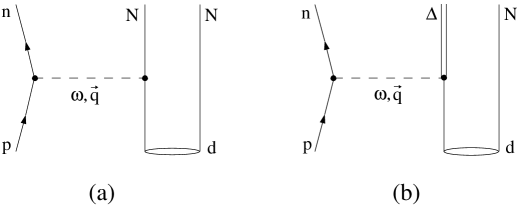
FIG. 1.: Impulse approximation diagrams for the ²H$(p,n)$ reaction. Here (a) shows the nucleon excitation and (b) the $\Delta$ excitation.

FIG. 2.: Direct term (a) and exchange term (b) of the $\Delta N$ potential $V_{\Delta\Delta}$. The mesons taken into account are the pion ($\pi$), the rho ($\rho$), the omega ($\omega$), and the sigma ($\sigma$).

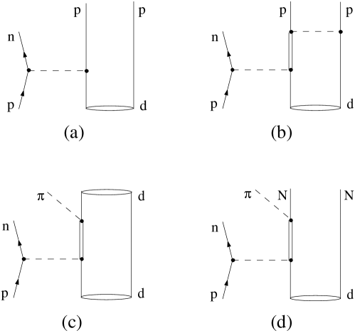
FIG. 3.: Reaction mechanisms of the different contributions to the inclusive cross section in our analysis. Only the lowest–order diagrams are shown. They represent: (a) quasi–elastic scattering, (b) p–wave rescattering, (c) coherent pion production, (d) quasifree $\Delta$ decay.

FIG. 4.: Differential cross section for the reaction ¹H$(p,n)\Delta^{++}$ at $T_{p}=790$ MeV and at scattering angles $\theta_{n}=0^{o}$,$7.5^{o}$, and $15^{o}$, respectively. The theoretical calculation uses the parameterization of $t_{NN,N\Delta}$ as given in App. A. Experimental data are from Ref. [32].

FIG. 5.: Zero degree neutron spectrum for the reaction ²H$(p,n)$ at $T_{p}=790$ MeV. The theoretical calculation (solid line) includes contributions from quasifree $\Delta$ decay (QF, dashed), coherent pion production (CP, dotted), and two–nucleon breakup of the deuteron (BU, dashed–dotted). Experimental data are from Ref. [32].

FIG. 6.: Full calculation with inclusion of baryonic exchange currents (solid line) in comparison with the “spectator approximation” result where $V_{\Delta\Delta}=V_{N\Delta}=0$ (dashed line). Experimental data are from Ref. [32].

FIG. 7.: Separation of the inclusive cross section into spin–longitudinal (LO, $\sim\vec{\sigma}\cdot\hat{q}$) and spin–transverse components (TR, $\sim\vec{\sigma}\times\hat{q}$). Experimental data are from Ref. [33].

FIG. 8.: Neutron spectra for the reaction ²H$(p,n)$ at $T_{p}=790$ MeV at scattering angles of $\theta_{n}=7.5^{o}$ and $\theta_{n}=15^{o}$, respectively. Experimental data are from Ref. [32].

FIG. 9.: Effects on coherent pion production ²H$(p,n\pi^{+})^{2}$H resulting from the direct (dir) and the exchange (ex) contribution of the $\pi$ meson to $V_{\Delta\Delta}$ (solid lines). The line labeled (dir+ex) shows the sum of direct and exchange contributions of the $\pi$. Note the apparent shift as compared to the dashed line which represents the spectator approximation $V_{\Delta\Delta}=0$.

FIG. 10.: Effects on coherent pion production ²H$(p,n\pi^{+})^{2}$H resulting from the $\pi$, $\rho$, $\omega$, and $\sigma$ meson contributions to $V_{\Delta\Delta}$ (solid lines). The line labeled ($\pi+\rho+\omega+\sigma$) represents the full model calculation. The dashed line shows the spectator approximation $V_{\Delta\Delta}=0$.

FIG. 11.: Effects of $V_{\Delta\Delta}$ on the exclusive cross section for coherent pion production (CP), quasifree $\Delta$ decay (QF), and deuteron breakup (BU). Calculations with (solid lines) and without $V_{\Delta\Delta}$ (dashed lines). Note the different scalings of the vertical axis.

FIG. 12.: Decomposition of the exclusive cross sections into contributions from unnatural parity states (UP) and natural parity states (NP). Calculations with (solid lines) and without $V_{\Delta\Delta}$ (dashed lines). Note the different scalings of the vertical axis.

FIG. 13.: Multipole decomposition of the zero–degree spectrum for the exclusive ²H$(p,n\pi^{+})^{2}$H reaction. Calculations with (solid lines) and without $V_{\Delta\Delta}$ (dashed lines) for three characteristical partial waves of the $\Delta N$ system are shown. Note the different scalings of the vertical axis.

FIG. 14.: Triple differential cross section for the ²H$(p,n\pi^{+})^{2}$H reaction at $\omega_{\text{lab}}=300$ MeV and $\theta_{n}=0^{o}$. The cross section is shown as a function of $\theta_{\pi}$ which is the angle between the outgoing $\pi^{+}$ and the momentum transfer $\vec{q}$ on the deuteron target.

FIG. 15.: Triple differential cross section for the ²H$(p,n\pi^{+})^{2}$H reaction in the spin–longitudinal (LO) and the spin–transversal (TR) channel. $M_{i}$ ($M_{f}$) refers to the spin–projection of the deuteron in the initial (final) state, hence the dashed curves labeled $M_{i}=M_{f}$ show a calculation where spin flips of the deuteron have been excluded.

REFERENCES

- [1] D. Contardo et al., Phys. Lett. B 168, 331 (1986).
- [2] D. A. Lind, Can. J. Phys. 65, 637 (1987).
- [3] C. Gaarde, Annu. Rev. Nucl. Part. Sci. 41, 187 (1991).
- [4] C. Gaarde, Nucl. Phys. A606, 227 (1996).
- [5] D. L. Prout et al., Phys. Rev. Lett. 76, 4488 (1996).
- [6] E. Oset, H. Toki, and W. Weise, Phys. Rep. 83, 281 (1982).
- [7] T. Udagawa, S. W. Hong, and F. Osterfeld, Phys. Lett. B 245, 1 (1990).
- [8] J. Delorme and P. A. M. Guichon, Phys. Lett. B 263, 157 (1991).
- [9] F. Osterfeld, Rev. Mod. Phys. 64, 491 (1992).
- [10] T. Udagawa, P. Oltmanns, F. Osterfeld, and S. W. Hong, Phys. Rev. C 49, 3162 (1994).
- [11] J. Chiba et al., Phys. Rev. Lett. 67, 1982 (1991).
- [12] T. Hennino et al., Phys. Lett. B 303, 236 (1993).
- [13] P. Oltmanns, F. Osterfeld, and T. Udagawa, Phys. Lett. B 299, 194 (1993).
- [14] B. Körfgen, F. Osterfeld, and T. Udagawa, Phys. Rev. C 50, 1637 (1994).
- [15] P. F. de Cordoba, J. Nieves, E. Oset, and M. J. Vicente-Vacas, Phys. Lett. B 319, 416 (1993).
- [16] P. F. de Cordoba, E. Oset, and M. J. Vicente-Vacas, Nucl. Phys. A592, 472 (1995).
- [17] O. V. Maxwell, W. Weise, and M. Brack, Nucl. Phys. A348, 388 (1980).
- [18] W. Leidemann and H. Arenhövel, Nucl. Phys. A465, 573 (1987).
- [19] J. A. Niskanen and P. Wilhelm, Phys. Lett. B 359, 295 (1995).
- [20] P. Wilhelm and H. Arenhövel, Nucl. Phys. A593, 435 (1995).
- [21] P. Wilhelm and H. Arenhövel, Nucl. Phys. A609, 469 (1996).
- [22] R. Schmidt, H. Arenhövel, and P. Wilhelm, Z. Phys. A355, 421 (1996).
- [23] S. S. Kamalov, L. Tiator, and C. Bennhold, Phys. Rev. C 55, 88 (1997).
- [24] A. M. Green, in Mesons in Nuclei, edited by M. Rho and D. H. Wilkinson (North–Holland Publishing Company, Amsterdam, 1979), Chap. 6, p. 258.
- [25] J. A. Niskanen, Nucl. Phys. A298, 417 (1978).
- [26] T.-S. H. Lee, Phys. Rev. C 29, 195 (1984).
- [27] T.-S. H. Lee and A. Matsuyama, Phys. Rev. C 36, 1459 (1987).
- [28] H. Pöpping, P. U. Sauer, and X.-C. Zhang, Nucl. Phys. A474, 557 (1987).
- [29] M. T. Peña, H. Garcilazo, U. Oelfke, and P. U. Sauer, Phys. Rev. C 45, 1487 (1992).
- [30] L. D. Fadeev, Zh. Eksp. Teor. Fiz. 12, 1014 (1961).
- [31] F. Blaazer, B. L. G. Bakker, and H. J. Boersma, Nucl. Phys. A590, 750 (1995).
- [32] D. L. Prout (private communication).
- [33] D. L. Prout et al., Nucl. Phys. A577, 233c (1994).
- [34] B. K. Jain and A. B. Santra, Phys. Rep. 230, 1 (1993).
- [35] Y. Jo and C.-Y. Lee, Phys. Rev. C 54, 952 (1996).
- [36] M. Lacombe et al., Phys. Rev. C 21, 861 (1980).
- [37] M. Lacombe et al., Phys. Lett. B 101, 139 (1981).
- [38] R. Machleidt, K. Holinde, and C. Elster, Phys. Rep. 149, 1 (1987).
- [39] G. E. Brown and W. Weise, Phys. Rep. C22, 281 (1975).
- [40] G. F. Chew and F. E. Low, Phys. Rev. 101, 1570 (1956).
- [41] C. A. Mosbacher, diploma thesis, University of Bonn, 1995 (unpublished).
- [42] X. Y. Chen et al., Phys. Rev. C 47, 2159 (1993).
- [43] H. Esbensen and T.-S. H. Lee, Phys. Rev. C 32, 1966 (1985).
- [44] G. Glass et al., Phys. Lett. B 129, 27 (1983).
- [45] C. Ellegaard et al., Phys. Lett. B 231, 365 (231).
- [46] J. S. O’Connell et al., Phys. Rev. C 35, 1063 (1987).
- [47] S. Boffi, C. Giusti, and F. D. Pacatti, Phys. Rev. 226, 1 (1993).
- [48] J. W. V. Orden and T. W. Donnelly, Ann. Phys. 131, 451 (1981).
- [49] C.-Y. Lee, Phys. Rev. C 55, 349 (1997).
- [50] T. Ericson and W. Weise, Pions and Nuclei (Clarendon Press, Oxford, 1988).
- [51] A. R. Edmonds, Angular Momentum in Quantum Mechanics (Princeton University Press, Princeton, 1957).