The longitudinal and transverse responses
in the inclusive electron scattering:
a functional approach

Abstract

The splitting between the charge-longitudinal and spin-transverse responses is explained in a model whose inputs are the effective interactions in the particle-hole channels in the frame of the first order boson loop expansion. It is shown that the interplay between $\omega$-meson exchange and box diagrams (two-meson exchange with simultaneous excitation of one or two nucleons to $\Delta$’s) mainly rules the longitudinal response, while in the transverse one the direct $\Delta$ excitations almost cancel the one-loop correction and the response is mainly governed by the $\rho$-meson rescattering inside the nucleus. It is also shown that a small variation in the nuclear densities may explain the observed discrepancies between different nuclei.

PACS 21.65, 25.30
Preprint GEF-TH-2/97

1 Short introduction

We will be concerned in this paper with the separation between longitudinal and transverse response in the inclusive electron scattering off nuclei. We shall present here a microscopic approach which naturally displays a depletion of the longitudinal and an enhancement of the transverse response.

Before entering the details of the model, some introductory words are required both concerning the experimental situation and the present status of the theoretical approaches – and we shall do that in sect. 2 – and the philosophy that provided us the guideline in constructing our theoretical frame. The latter topic, together with the modifications the phenomenology suggested in our line of thought, is resumed in sect. 3.

Next the bosonic loop expansion formalism, although already described in [1], will be resumed, for ease of the reader, in sect. 4. There particular emphasis is put on the presence of $\Delta$’s inside the diagrams.

Section 5 describes the mean field approach. While in the charge longitudinal channel this approximation level is too poor both for its disagreement with the data and for its poor dynamical content, in the transverse one it is able to provide us information about the effective interaction in the isovector spin-longitudinal effective interaction, that is one of the phenomenological inputs of our model, and this because of an accidental almost complete cancellation of the 1-loop corrections in this channel.

In sect. 6 the one-loop corrections are described and it is shown how the presence of the $\Delta$’s can distinguish the response in the two channels.

Finally in sect. 7 our conclusions are drawn.

2 The experimental and theoretical situations

The experimental outcomes in the quasi-elastic peak (QEP) region are at present still controversial both on the experimental and theoretical point of view. Starting from the usual relation

$$\frac{d^{2}\sigma}{d\Omega d\epsilon}=\sigma_{M}\left\{v_{L}R_{L}(q,\omega)+v_{T}R_{T}(q,\omega)\right\}$$ (1)

the Saclay experimentalists [2, 3] where first able to perform the Rosenbluth separation, thus getting both $R_{L}$ and $R_{T}$. The outcomes are known: the longitudinal response, to whom a great amount of work has been devoted in these last years (see for instance ref. [4] for a wide review of the current literature), came out to be drastically quenched with respect to the Free Fermi Gas (FFG) model, while the transverse one was remarkably increased, a fact, this last, which instead has been less emphasized.

The first difficulties with this Rosenbluth separation came from the non-fulfillment of the Coulomb sum rule and the connected problem of the so-called missing strength. In fact, the integrated longitudinal response, expected to provide the nuclear charge, was quenched by a, say, 10% in case of Carbon but by a 40% in the case of Calcium. More recent data from Saclay, taken on Lead, showed and even enforced the same trend, the sum rule being reduced to about a 40% of the total charge [5].

Few years ago the Rosenbluth separation has also been performed on the data taken in two different experiments at Bates and the longitudinal responses have been published [6]. The quenching of the sum rule for the ${}^{40}Ca$ turns out to be, in this case, of about a 10%, in sharp contrast with the Saclay data.

Very recently, by reviewing the world data of inclusive electron scattering, Jourdan [7] outlined that the Rosenbluth separation is not free from theoretical ambiguities, and other are introduced in deriving the sum rule: just to exemplify, the one-photon approximation is questionable for heavy nuclei and the distortion of the outgoing electron must be correctly accounted for, before separating the longitudinal and transverse channels; furthermore, relativity prevents us to define the Coulomb sum rule in a natural way [8] and some ad hoc relativistic corrections are required; moreover the contributions from experimentally unexplored or physically unaccessible regions in the high energy tail of the response must be correctly accounted for. By considering all these topics (and others neglected here for sake of brevity) Jourdan showed that the corrected sum rule derived from world set of data is compatible with $Z$ within a 1% incertitude.

This outcome is, in principle, not strongly contradictory with the Saclay results: the nonrelativistic Coulomb sum rule in fact properly reads

$$\int\limits_{0}^{\infty}\frac{RE_{L}(q,\omega)}{G_{E}^{2}(q^{2})}\simeq S_{L}(q)=Z+\frac{2Z}{\rho}g(q)\;,$$ (2)

$g(q)$ being the pair correlation function, and the outcome of [7] only states that $g(q)$ is compatible with 0 at, say, $q=$570 MeV/c (the largest transferred momentum examined there). In ref. [9] it is shown indeed that at lower momenta still a sizeable quenching (even if less pronounced than in [2, 3]) survives.

Waiting for new experimental data that would (hopefully) solve the present contradiction, we followed, as a guideline, the Saclay data, plotting however, if available, also the data from Bates and those derived from the world data set according to [7, 9].

To better explain this choice, let us anticipate a little the topics of sects. 3 and 4: in order to determine a form for the effective interaction and then to perform numerical calculations we need to refer to some phenomenological inputs. In this respect Saclay data display a wide range of transferred momenta both in the longitudinal and transverse channel, while those from Bates are limited, up to our knowledge, to the longitudinal response only and cannot be used to set our inputs. We will see, instead, that the data of refs. [7, 9] can also be obtained by slightly alter our parametrization, but without destroying the physical picture we are going to derive in the following. The physical interpretation however will change significantly. We defer to the conclusion a more complete discussion about this point.

Coming now to the theoretical side of the problem, to our knowledge the longitudinal response has been extensively investigated, while the transverse still requires much attention.

Concerning the former, all theoretical approaches, based on a variety of dynamical models, agree in providing a more or less pronounced depletion of the QEP in the longitudinal channel [10, 11, 12, 13]. The different physical inputs and even the different languages present in the quoted (and many other) papers seem however to prevent a clear comparison between them.

The transverse response has been instead less investigated. The common trend seems to be the need of including at least two particles-two holes excitations to describe the QEP and dip region together [13, 14, 15]. In particular ref. [13] seems to be (up to our knowledge) the only attempt to explain simultaneously the two responses within the same frame, namely that of continuum RPA plus two-body currents. Still, both responses seem to be slightly overestimated. Further, as in finite nucleus calculations, the use of the phenomenological Skyrme interaction obscures the link with the underlying dynamics. On the other hand the dynamically richest approach is provided in our opinion by the FHNC calculations [10] but in this case the possibility of exploiting the transverse response is precluded by the difficulty (only for the moment, we hope [16, 17, 18]) of embedding pions and $\Delta$’s in a variational approach, which in turns forbids the inclusion in the calculation, at least in a natural way, of the Meson Exchange Currents (MEC).

Furthermore, the exact preservation of the sum rules, gauge invariance and other general theorems is not in general ensured by the usual many-body techniques. Thus some more efforts in explaining the two responses are still required.

3 The theoretical frame

Having shortly revisited the experimental and theoretical situation, let us spend a few words about the philosophy underlying our approach [1, 19].

Our starting point in [20] was to build up a well-behaved approximation scheme for a system of nucleons and pions.

By one side ”well-behaved scheme” means an expansion of the physical quantities we are looking for, whatever they are, in powers of a given parameter. This because the unicity of the Taylor expansion automatically preserves all those sum rules and general theorems that can be expressed by the action of linear operators (integrations, Fourier transforms, functional derivatives and any other) over the generating functional (see, e.g., [21]).

On the other side, a system of nucleons and pions seemed to us a good laboratory to study how a renormalizable quantum-field-theoretical model embeds into a many-body problem.

The idea of bosonization arose quite naturally there, as it was obtained by representing the generating functional of the system by means of a Feynman path integral and by explicitly integrating over the fermionic degrees of freedom. Then the system turned out to be described by the bosonic effective action

$$S_{B}^{\rm eff}=\frac{1}{2}\int d^{4}x\,d^{4}y\,\phi(x)\left[D_{0}\right]^{-1}(x-y)\phi(y)$$

$$-\sum_{n=2}^{\infty}\int d^{4}x_{1}\dots d^{4}x_{n}\frac{1}{n}\Pi^{(n)}(x_{1},\dots,x_{n})\phi(x_{1})\dots\phi(x_{n})\;,$$

$\phi$ denoting the pion field (isospin is neglected for simplicity), $D_{0}$ its free propagator and the highly non-local vertices $\Pi^{(n)}(x_{1},\dots,x_{n})$, that keep memory of the fermion dynamics, being shown diagrammatically in fig. 1.

Figure 1: The bosonic effective action. Dots denote the external points $x_{i}$ while solid lines stand for in medium free nucleon propagators.

This action generates a new class of approximations – or a recipe to collect classes of Feynman diagrams together – when the semiclassical expansion is carried out. This scheme is also referred to as boson loop expansion (BLE). Its renormalizability has been proved in [22].

The practical recipe to classify a Feynman diagram according to its order in BLE is to shrink to a point all its fermion lines and to count the number of boson loops left out.

Thus the mean field level of the theory just coincides with the RPA (or, better, with the ring approximation, without antisymmetrization). This can be seen either diagrammatically, according to the above rule, or observing that the quadratic part of the action just contains the inverse ring propagator, namely $\frac{1}{2}D_{0}^{-1}-\frac{1}{2}\Pi^{(2)}\;.$ Note that $\Pi^{(2)}$ coincides, up to factors, with the Lindhard function. The present unusual notation is chosen to agree with refs. [23, 24].

Figure 2: First order diagrams in the BLE. Recall that the dashed lines always describe RPA-dressed bosons

At the linear response level the mean field is thus described by the RPA-dressed polarization propagator if the probe has the same quantum numbers of the pion or, if not, by the bare Lindhard function.

At the one-loop order the only possible diagrams (we neglect here the MEC, since we shall not be concerned with them in the rest of the paper) are those of fig. 2. We remind once more that all bosonic lines have to be seen as RPA-dressed.

To be more specific, the full response at the one-loop order is given (up to factors) by the imaginary part of the diagrams of fig. 3, where the black bubble denotes the sum of all the diagrams of fig. 2.

Figure 3: Diagrams pertaining to the response function at the one-loop level. The black bubble summarizes the 5 diagrams of fig.2; we explicitly indicated the RPA dressing of the bare meson propagators (dashed lines).

It is evident from fig. 2 that only fermion loops with at most four external legs intervene at the one-boson-loop order. This fact is of overwhelming relevance since analytical expressions are available for them [23, 24], at least in the nonrelativistic kinematic.

This occurrence makes the calculation feasible and in ref. [25] we got some preliminary results for the longitudinal response on the QEP, the only dynamics being there the pion exchange. A very tricky technicality forced us to consider static pions only. We are not able at present to perform a relativistic calculation because the outcomes of [23, 24] cannot be fully translated to a relativistic frame. It is well known that the pion branch in the RPA scheme is coupled to the particle-hole mode. Within a nonrelativistic nucleon kinematics, in a momentum range around 1.6 GeV/$c$, the pion branch enters the particle-hole (p-h) continuum, because the former is relativistic and the latter is not. This originates wild oscillations which are by one side absolutely unphysical, but on the other numerically unavoidable. Thus we were forced to accept a static version of the pion exchange potential – at least for the moment: some promising work is in progress to overcome this limitation.

Further, the pion condensation is unavoidably met in the RPA scheme if we only allow pion exchange without accounting for short range correlations (SRC). Since pion condensation, if any, occurs very far from nuclear matter stability region, we are again forced to forbid its occurrence by phenomenologically embedding SRC in our model by means of the Landau parameter $g^{\prime}$, which resumes all the complicated short range p-h interactions in the pion channel.

To adhere to phenomenology we are thus forced to change somehow our approach, both in the formalism and the underlying philosophy.

Concerning the former we must give up a field theory and adopt a potential frame. The derivation of the response at the one loop level is given in detail in ref. [1] and will not be repeated here. We only remind the reader that a Hubbard-Stratonovitch transformation [26, 27, 28] bosonizes a potential theory, leading to an effective action coincident with (3) up to a redefinition of the symbols: $D_{0}^{-1}$ is replaced by the inverse potential in the given p-h channel and the field $\phi$ is reinterpreted as an auxiliary field. The topology of the diagrams remains unchanged.

To exemplify we used in [25] the effective interaction

$$D_{0}(q)\longrightarrow V_{\pi}(q)={f^{2}_{\pi NN}\over m_{\pi}^{2}}\left\{g^{\prime}_{L}({\bf q})-{{\bf q}^{2}\over m^{2}_{\pi}+{\bf q}^{2}}\right\}v_{\pi}^{2}(q^{2})\;,$$ (4)

where the function $g^{\prime}_{L}({\bf q})$ embodies the SRC.

Leaving aside technicalities (discussed, on the other hand, in [1, 25]) eq. (4) deserves some conceptual comments. Not only in fact we were forced to abandon a field-theoretical model, but the parametrization of SRC also implies the replacement of a realistic potential with an effective one, ruled by the Landau parameter $g^{\prime}_{L}$.

The usual scheme where the Landau-Migdal parameters are used is, in our language, the mean field level; this approximation underlies also the phenomenological analyses used to substantiate them (see for instance [29]). We are working now at a deeper level, namely the one-boson-loop one. Here the need of the Landau-Migdal parameters still survives, but they cannot be directly derived from the same phenomenology. The occurrence in a diagram of two subsequent Landau parameters renormalizes their value. Thus we are not linked to preserve the same values as at the mean field level but we should look to them as to free parameters able to reproduce the experimental data.

In practice we attempted, as far as possible, to maintain some connection with the known phenomenological analyses. This should be mandatory in a purely nucleonic scheme because if the loop expansion is convergent, then the parameters redetermined at the 1-loop order should be not so different from their corresponding mean field values. The presence of intermediate states with one or more nucleons excited to $\Delta$’s changes qualitatively the previous statement, as is the case for the so-called “box diagrams”. We will discuss better this point in the following. Thus ultimately we introduced as phenomenological ingredients of our models the effective interactions in the various channels to reproduce reasonably well the longitudinal and transverse response functions, nevertheless trying to preserve some adherence to the Landau parameters as fixed at the mean field level when no other indications are available.

However, in going from the mean field to the one loop level, a qualitative change is met. In fact in the former case not too high momenta (i.e., of the order of the momentum of the probe) enter the dynamics, while in the latter the bosonic loop momentum is integrated over and the high momentum behaviour of the effective interaction rules the convergence of the integral (see, e.g., [30] for a more detailed discussion). This is exploited in (4) by forcing a $q$-dependence in $g^{\prime}_{L}$ such that

$$g^{\prime}_{L}(q)\stackrel{{\scriptstyle q\to\infty}}{{\longrightarrow}}1\;,$$ (5)

in order to account for SRC. But this in turn requires the introduction of a further cut-off related to the SRC range that becomes the crucial parameter ruling the one loop corrections.

These last considerations set the philosophy underlying our approach. To resume, the effective interaction is a phenomenological input, to be fixed, as far as possible, on the experimental data. Two quantities characterize the effective interaction, namely $g^{\prime}$ (taken at $q\to 0$), which mainly governs the response at the mean field level, and the cut-off which sets the behaviour of the effective interaction at high momenta, which instead determines the size of the one-loop corrections.

So far we have only discussed a system of nucleons and only one effective interaction. Needless to say, the dynamics required to describe the nuclear responses is by far richer. Formally our approach remains unchanged and other channels are accounted for by simply interpreting the dashed lines in figs. 2 as a sum over all the allowed channels, as we shall discuss in the next section.

Also, the excitation of the nucleons to a resonance (in the present paper we will be concerned with the $\Delta_{33}$ only) can be allowed by interpreting each solid line as a nucleon or as a $\Delta$ and again summing over all possible cases. Remarkably the topology of the diagrams does never change. Simply, conservation laws will kill some of them.

4 The dynamical model

To substantiate the theoretical frame discussed in the previous section, we need to define the dynamics we are going to consider. In this respect, three topics, namely the effective interactions, the diagrammology – with particular attention to the excitation of a $\Delta$-resonance – and the external current characterize the model.

In the above we confined ourselves, just to simplify the exposition, to a very poor scheme, because the extension to a richer dynamics is formally trivial. The same cannot be said however about the physical content.

In ref. [25] we evaluated the longitudinal response using the effective interaction (4) in the pion channel. The results were qualitatively unsatisfactory, but they went in the right direction. A more sophisticated approach was pursued in [1]: the formalism is the same, but other channels are considered. We focused there our attention on the pion channel, the $\rho$ channel and the transverse $\omega$ channel. We neglected the scalar channels following the indications of Speth et al. [29] that suggest there a weak or vanishing effective interaction. Of course this outcome is questionable and was adopted in [1] only for sake of simplicity. The statement of ref. [29] refers in fact to the mean field level, while at the one loop order effective interactions may exist able to lead, owing to cancellations between them and to the interference with the mean field level, to the same phenomenological outcome of ref. [29]. At the mean field level, in fact, the statement that the effective interaction in a given spin–isospin channel is small means that the linear response in the chosen channel is close to the one of the FFG. At the one loop level instead the effective interaction in a given channel can affect the responses in all the other ones. Thus we must build up a coherent set of effective interactions in all the channels such that, for instance, in the scalar channels the global effect of the mean field and of the one loop corrections cancel together, being however both not necessarily small. Further, the excitation of a nucleon to a $\Delta$-resonance was only partially accounted for (and largely underestimated) in [1]. It will play instead a central role in the present paper.

We shall consider here the (correlated) exchange of $\pi$, $\rho$ and $\omega$-mesons. In each particle-hole channel the interaction will read

$$V_{m}(q)={f^{2}_{\pi BB^{\prime}}\over m_{\pi}^{2}}\left\{g^{\prime}_{m}({\bf q})-C_{m}{{\bf q}^{2}\over m^{2}_{m}+{\bf q}^{2}}\right\}v_{m}^{2}(q^{2})\;,$$ (6)

where the index $m$ runs over the accounted channels and $B=N$ or $\Delta$.

Concerning the pion, it propagates in the isovector spin-longitudinal channel. Since the pion exchange is not far from being perturbative, its coupling constant is not assumed to be renormalized in the medium and hence, by definition, $C_{\pi}=1$.

A vector meson interact with the nucleons by means of the relativistic lagrangian

$$g\overline{\psi}\gamma_{\mu}\psi\phi^{\mu}+\frac{f}{4m}\overline{\psi}\sigma_{\mu\nu}\psi(\partial^{\mu}\phi^{\nu}-\partial^{\nu}\phi^{\mu})$$ (7)

where the first term is a standard coupling to a current while the second term describes an “anomalous magnetic moment”. According to the analyses of ref. [31] this last term is absent in the $\omega$ case but dominates the $\rho$-exchange.

Obviously the interaction (7) generates a convective and a spin current coupled to the 3-vector part of the mesonic field plus a scalar coupling to its time component. Customarily the convective current is neglected. Thus we are left with an interaction in the spin-transverse channel coming from the spin current and one in the scalar channel coming from the coupling to $\phi^{0}$. Since the “anomalous magnetic moment” is absent in the $\omega$ case, the coupling constants of these two interactions would coincide, while the scalar component of the $\rho$ is coupled much more weakly than its 3-vector part.

Coming now to the effective interactions to be put in our machinery, we adopted for the $\rho$ case the same coupling constants as in the Bonn potential [31], corresponding to a $C_{\rho}\sim 2.3$ in the isovector spin-transverse channel and to $C_{\rho}\sim 0.05$ in the scalar isovector one, and this because, in spite of its large coupling the $\rho$-exchange is perturbative too due to the high mass of the $\rho$ itself. Further, in the spin-transverse channel we need to introduce SRC, because in the Landau limit the effective interaction must equal the one of the spin-longitudinal channel, and this makes by far non-perturbative the whole effective interaction. We shall see later that the particular form of this interaction plays a crucial role in explaining the responses. We shall also account for the interaction of the $\rho$ meson with the nuclear medium other than ph and $\Delta$h excitations (we means for instance $\rho\to\pi\pi$ with further interaction of pions with the medium) by attributing to the $\rho$ (in the spin-transverse channel only) an effective mass to be specified later. In the scalar isovector channel no Landau parameter has been added and the mass is left unchanged.

Coming to the $\omega$ mesons, we have left the interaction in the isoscalar spin-transverse channel unchanged, since it is weak, but the scalar isoscalar channel needs to be renormalized drastically, because there the effective interaction is made by the exchange of many $\omega$ mesons. Since we have no sufficiently striking experimental information on the details of this effective interaction we have simply taken the corresponding $C_{\omega}$ as a free parameter, without changing nor the functional form neither its range. In order to avoid uncontrolled complications no Landau parameters have been added in these two channels.

The Landau parameter $g^{\prime}$ is thus present in the isovector spin-transverse and spin longitudinal channels only, where it has been parametrized according to

$$g^{\prime}_{L,T}(q)=C_{m}+(g_{0}^{\prime}-C_{m})\left[{q_{c\,{L,T}}^{2}\over q_{c\,{L,T}}^{2}+q^{2}}\right]^{2}$$ (8)

in such a way that for $q\to 0$ $g^{\prime}_{L,T}(q)\to g^{\prime}_{0}$ and for $q\to\infty$ a proper generalization of condition (5) is respected, namely

$$g^{\prime}_{L,T}(q)\stackrel{{\scriptstyle q\to\infty}}{{\longrightarrow}}C^{T=1}_{L,T}\;.$$ (9)

The further cut-offs are called here $q_{c\,{L,T}}$. The form we assumed for the effective interaction is not qualitatively different from other widely employed in the literature (see for instance [32, 33]), the only true change being that the value at ${\bf q}=0$ is in our approach free. Up to our knowledge there is no experimental input to fix $q_{c\,L}$, but it is commonly assumed of the same order of the $\omega$ mass (and hence of the inverse radius of the repulsive core in the nucleon-nucleon interaction) and many calculations using this value have been performed successfully [34, 35]. No indications are available instead for $q_{c\,T}$. Some possible choices are discussed in [19], but since the interaction in the $\rho$-channel dominates the responses, as we shall see below, we defer its description to the subsequent sections.

The vertex function present in (5) is customarily assumed to be

$$v_{m}(q^{2})={\Lambda_{m}^{2}-m_{m}^{2}\over\Lambda_{m}^{2}+{\bf q^{2}}-q_{0}^{2}}$$ (10)

but in our calculation has been assumed as static too for sake of coherence.

Next we come to the role of the $\Delta$-resonance. The diagrammology, as far as its topological content is concerned, follows quite simply from fig. 2, by allowing each line to be either a nucleon or a $\Delta$. Isospin conservation rule cuts some diagram but too many of them survive. They are displayed in figs. 4 to 6.

Figure 4: The self-energy diagrams with inclusion of $\Delta$-resonances. The $\Delta$’s are described by thick lines

Fig. 4 expands the first and second diagram of fig. 2 (self-energy terms), fig. 5 expand the third one (exchange) and fig. 6 the last two diagrams (correlation terms). Note that these are obtained by expanding both the two bubbles present there. Since each bubble translates into 7 possible diagrams, then 49 of them arise for each of the two terms accounted for.

Figure 5: The exchange diagrams with inclusion of $\Delta$-resonances. The $\Delta$’s are described by thick lines

In figs. 4 to 6 only the isospin conservation law has been considered.

Figure 6: The correlations diagrams with inclusion of $\Delta$-resonances. The diagrams are obtained by combining each component of the upper line with each piece of the lower one. The $\Delta$’s are described by thick lines

The above shown diagrammology deserves some comments concerning the feasibility of the calculation. There are in fact a total of 125 Feynman diagrams (14 self-energy, 15 exchange and 98 correlation diagrams). Since we consider five different effective interaction, any dashed line should be counted 5 times, giving thus a total a 2595 diagrams. To understand the relevance of the results of refs. [23, 24] in enabling us to truly evaluate all of them consider the following: the usual way of computing them is to reduce each one to Goldstone diagrams by explicitly performing the frequency integration. In the present case the integration over the bosonic frequency cannot be simply performed, due to its RPA-dressing. Would it be even possible, due to the all the occurring time ordering that must be accounted for, one should end up with 1767480 (!) diagrams almost all containing 9-dimensional integrals with extremely complicated boundaries. In any case, a hopeless task.

Refs. [23, 24] tell us that the integrals over the fermionic loops can be performed analytically provided we sum up all the Goldstone diagrams, i.e., at the Feynman diagram level. This not only shortcuts the number of diagrams, coming back to the 2595 ones quoted before, but it reduces the numerical integrations to the bosonic loop only. Since here one integration is trivial we are left out in practice with 2595 3-dimensional integrals, a tedious but not impossible job (as an aside, further tricks have been of course used so to reduce both the computing time and the structure of the calculation by parallelizing the integration procedure and by exploiting the regularities of the diagrams, so to reduce the codes to a manageable form and the computing time to a reasonable order – to say, one day for a complete calculation with one set of parameters on a last generation $\alpha$-VAX).

Still the Feynman rules have not been fully determined.

First we need to define the $\Delta$ propagator, and this is done by setting

$$G_{\Delta}(p)=\frac{1}{p_{0}-\frac{{\bf p}^{2}}{2M_{\Delta}}-\delta M+i\eta}$$ (11)

($\delta M$ being the mass difference between $\Delta$ and nucleon), without accounting for the $\Delta$ width. This is correct for two reasons: first, the width is frequency and momentum dependent and it has of course a threshold at the pion mass in the $\Delta$ rest frame and since the $\Delta$ lives almost always below this threshold, the width is coherently set to 0; second, in the BLE the $\Delta$ width comes out – at least partially – from a one-boson-loop correction, like, e.g., in the diagram 1e) of fig. 4 and, if any, is already accounted for.

A second need in order to evaluate the Feynman diagrams is to define the vertices. They carry in fact some spin-isospin matrices: in the $N$-$N$ vertex a spin-longitudinal potential brings with it a factor ${\bf q}\cdot{\mbox{\boldmath$\sigma$}}$ while a spin-transverse one has the factor ${\bf q}\times{\mbox{\boldmath$\sigma$}}$ and of course an isovector potentials adds to them a factor $\tau_{i}$; in a $N$-$\Delta$ vertex the Pauli matrices $\sigma$ and $\tau_{i}$ are replaced by the corresponding transition matrices $\bf S$ and $T_{i}$ [36] and finally in the case of the $\Delta$-$\Delta$ vertex we need the less known 3/2–3/2 spin matrices, denoted here by $\cal S$ and ${\cal T}_{i}$. They are displayed in appendix A.

As a matter of fact we do not need their explicit expression, but only the trace of at most four of them. The traces needed to evaluate the spin-isospin part of our diagrams are also given in the appendix A. The traces have to be evaluated for each of the 2595 Feynman diagrams and for the longitudinal and transverse isoscalar and isovector responses: actually the job is not so tedious as it could seem, owing to the many symmetries in the diagrams: the main ingredients needed to construct them are given in appendix B. These factors have been anyway checked out for maximum safety with an analytical calculation performed with the Mathematica code.

The last topic we need to discuss in order to complete the description of the model is the form of the e.m. current. It acts on three different sectors, namely the $N$-$N$, the $N$-$\Delta$ and the $\Delta$-$\Delta$ ones and can be separated into the longitudinal and transverse channel and, further, in its isoscalar and isovector components.

In the longitudinal channel, the simplest one, we account for the $N$-$N$ and $\Delta$-$\Delta$ charge operators but of corse not for $N$-$\Delta$ transitions. We have chosen the following form for the matrix elements of the charge operators:

$$<N|\rho|N> = \frac{1}{2}\tilde{G}_{E}^{T=0}+\frac{1}{2}\tau_{3}\tilde{G}_{E}^{T=1}$$ (12)

$$<\Delta|\rho|\Delta> = \frac{1}{2}\left(1+{\cal T}_{3}\right)\tilde{G}_{E}^{\Delta}\;.$$ (13)

Here the $\tilde{G}_{E}$ are defined as

$$\tilde{G}_{E}=\frac{G_{E}}{\sqrt{1+\tau}}$$ (14)

to account for the recoil, according to [37]. In the nucleon case the familiar Sachs form factors are employed, while in the $\Delta$ case no experimental evidence can be invoked to select between different theoretical models. We have chosen here for $G_{E}^{\Delta}$, as a reasonable compromise, the dipole form, which should better account for the high momentum tail, with the radius coming from the constituent quark model [38], where it comes out to be a 27% higher than the one of the nucleon. We correspondingly increase the cut-off in the dipole form factor of the same amount.

The current matrix elements instead has a more complicated structure. In the nucleonic sector we are forced to the shortcut of dropping the convective part of the current by putting

$$<N|{\bf j}|N>=i\frac{{{\mbox{\boldmath$\sigma$}}}\times{\bf q}}{2m}G_{M}\;.$$ (15)

The transition current for the single nucleon is written very simply in the centre-of-mass frame. We retain the $M1$ component only, so that the current reads

$$<N|{\bf j}|\Delta>\bigm{|}_{\rm c.of.m.}=i\mu_{N\Delta}T_{3}\frac{{\bf S}\cdot{\bf q}\times{{\mbox{\boldmath$\epsilon$}}}}{2m}G_{M}^{\Delta}\;;$$ (16)

we need however in our calculations, to be able to use the results of refs. [23, 24], an equivalent expression in the laboratory frame. The transformation of (16) to the laboratory frame generates a convection part, which is forcedly neglected, and, to the lowest order in the non-relativistic expansion, the replacement

$${\bf q}\to\frac{m}{m+\omega}{\bf q}\;.$$ (17)

Finally the current in the $\Delta$ sector is written as

$$<\Delta|{\bf j}|\Delta>=i\mu_{\Delta}\frac{1+{\cal T}_{3}}{2}\frac{{{\mbox{\boldmath$\cal S$}}}\times{\bf q}}{2m}G_{M}^{\Delta}$$ (18)

where $\mu_{\Delta}=2.95$ according to [38] and again, both in (16) and (18) we have taken $G_{M}^{\Delta}$ in dipole form with the same radius as $G_{E}^{\Delta}$.

A relevant issue of the present work is that the transition current is present in the magnetic channel but not in the charge-longitudinal one. This seemingly trivial consideration implies the highly nontrivial consequence that many of the displayed diagrams are killed in the charge-longitudinal channel. More explicitly only the diagrams 1a), 1c) and 1g) survive in fig. 4 (and the same happens to the second self-energy diagram of fig. 2), in the exchange diagram only 3a), 3h), 3k) remain and finally in the correlation diagrams only the combinations of 4a), 4c) and 4g) with 4a’), 4c’) and 4g’) are allowed. This means that 21 diagrams (including self-energy and exchange) survive in the longitudinal channel while all 127 diagrams survive in the transverse one.

Thus we realize in practice what argued in ref. [39], where it was outlined that the so called “swollen nucleon” hypothesis, which is channel-insensitive in a bag model, becomes channel-dependent when the mesonic cloud is accounted for. Here the channel dependence comes out at the one-loop level and is represented by the many diagrams allowed only in the transverse response. They individually could well contribute by a very small amount, but their large number provides at the end of the calculation a non-negligible result.

5 The mean field level

The mean field level in a coherent discussion is expected to precede the first order corrections, and we shall follow this aptitude in the present exposition. The situation at hand is particularly unlucky however, because the mean field level is inextricably linked in the present case to the one-loop corrections. In fact:

1. In the charge-longitudinal channel the mean field is mainly dominated by the $\omega$ exchange, which is repulsive and so entails a quenching of the response. As a simple mathematics shows, this implies also a hardening of the response [40] not observed in the data. Further, we neglect the $\sigma$-meson exchange, which is known from the Dirac phenomenology [41, 42, 43] to be attractive and that cancels to a large amount with the $\omega$ exchange. In our approach, in the same line of thought of the Bonn potential,[31, 44] the $\sigma$-meson is replaced by the box diagrams, i.e., two meson exchange with simultaneous excitation of one or two nucleons to a $\Delta$ resonance. These diagrams are contained indeed in our correlation diagrams, which are however at the one-loop level.

2. In the following section we will show that in the transverse channel the one-loop corrections are strongly suppressed (we shall see there that the $\Delta$-excitation makes this job). Thus the mean field becomes dominant in explaining the response and it is conversely ruled by the effective interaction in the $\rho$ channel. Thus, owing to this outcome, we can directly extract information about the effective interaction from the data, at least in this spin–isospin channel.

Let us now shortly review the present phenomenology and compare it with a FFG calculation.

Figure 7: Mean field calculation for the charge longitudinal response on ${}^{12}C$ at different transferred momenta. Solid line: mean field; dashed line: Free Fermi Gas. Data from [2, 3] (circles) and from [7, 9] (triangles). In the calculations we assumed ${k_{F}}=1.10$ fm^-1

We displayed in fig. 7 the mean field previsions for the charge longitudinal response for ${}^{12}C$ at different transferred momenta and the same is done for ${}^{40}Ca$ in fig. 8

Figure 8: Mean field calculation for the charge longitudinal response on ${}^{40}Ca$ at different transferred momenta. Solid line: mean field; dashed line: Free Fermi Gas. Data from [2, 3] (circles), from [7, 9] (triangles) and from [6] (boxes). In the calculations we assumed ${k_{F}}=1.2$ fm^-1

A common trend comes out clearly, namely that the FFG is not able to explain the responses at low $q$. The RPA dressing is carried out with $C_{\omega}$=0.15 and $C_{\rho}$=0.05: its effect is clearly weak, but induces a remarkable hardening of the response. At higher $q$ instead the FFG becomes more and more suitable. We interpret this outcome as an evidence that correlations (both short-ranged and RPA-induced) are fading away, in agreement with our theoretical previsions – again, as we shall see in sect. 6.

The situation of ${}^{40}Ca$ deserves a further comment. The FFG fails to reproduce the data at $500MeV/c$, those data being taken at Saclay. Remarkably in the Rosenbluth separation of Jourdan[9] there is a qualitative agreement with the results of Saclay at $300MeV/c$ while at higher momentum transfer the longitudinal response significant discrepancies arise. And in fact the Jourdan data on ${}^{40}Ca$ at $570MeV/c$ are in good agreement with the free Fermi gas model, thus following the same trend of ${}^{12}C$.

The situation is drastically different in the transverse channel. There the effective interaction is carried by $\rho$-meson exchange (attractive) plus SRC (repulsive). It is evident from figs. 10 and 11 that the FFG fails badly even at high momentum transfer. Here we do not expect a big contribution from the MEC (that part of them, at least, which is not yet embodied in our model, like, e.g., direct $\Delta$ excitation) at least in the left side of the QEP. This onset is supported by the occurrence of the $y$-scaling in this region. The pion-in-flight contribution is in fact associated to the breaking of $y$-scaling, and experiments show its occurrence only in the right side of the QEP (see for instance the review [45]). Thus the deformation of one half of the peak has to be attributed either to the effective interaction in the channel of the $\rho$ or to one-loop corrections. Let us assume, for the moment without proof, that the former case occurs.

If so, the transverse response has the form

$$R_{T}=-\frac{1}{\pi}\Im\frac{\Pi_{T}^{T=1}}{1-V_{\rm eff}^{T=1}\Pi_{T}^{T=1}}$$ (19)

(we have neglected here the $T=0$ for sake of simplicity, since it represent at most a 3% of the total; in our calculations however this component is also accounted for). $\Pi_{T}$ denotes the transverse component of

$$\Pi_{\mu\nu}(x,y)=<\Psi_{0}|T\left\{j_{\mu}(x),j_{\nu}(y)\right\}|\Psi_{0}>$$ (20)

and $V_{\rm eff}^{T=1}$ is the effective interaction in the $\rho$-channel. It is well known [40] that an attractive effective interaction enhances the response, while a repulsive one depletes it. Experimental data shows, in the case of ${}^{12}C$, that for $q=300~{}MeV/c$ the FFG is roughly sufficient to describe the data, while at higher values it systematically underextimate them. Thus in order to meet the experimental situation an effective interaction is required such to vanish around $q=300~{}MeV/c$ and to be attractive in higher $q$-regions.

In the form we have chosen the attractive part of the effective interaction comes from the true $\rho$-exchange and the repulsive one from the SRC. We must keep in mind however that this is simply a parametrization for the effective interaction, which is instead an unknown as a whole. To maintain the form (6) and reasonable values for $g^{\prime}_{T}$ and $C_{\rho}$ we have slightly changed the $\rho$-mass, attributing to it an effective value of $600~{}MeV$. This by one hand is not unreasonable, as the $\rho$ itself, either directly or when it lives as a pion pair, feels the effect of the nuclear medium, which consequently renormalizes is mass. On the other hand, however, we want to stress that unusual parameters in (6) could look badly, but they do not disturb too much provided the whole effective interaction looks reasonable.

The parameters which seem to better describe the transverse response are: $m_{\rho}=600~{}MeV$, $g^{\prime}_{0}=0.35$, $q_{c,T}=1.3~{}GeV/c$, $C_{\rho}=2.3$, $\Lambda=1.75~{}GeV/c$ (making here the universal choice, i.e., keeping all the $C_{\rho}$ equal). With this choice the tail of the interaction is quickly decreasing so that the expected enhancement of the response at high transferred momenta is missing, but a milder behaviour of the tail would overemphasize the one loop corrections.

The effective interaction in the $\rho$ channel is shown in fig. 9, together with the one we employed in ref. [19] ($m_{\rho}=770~{}MeV$, $g^{\prime}_{0}=0.5$, $q_{c,T}=1.4~{}GeV/c$, $C_{\rho}=2.2$, $\Lambda=2.5~{}GeV/c$). We remark, as already outlined in [19], that this effective interaction is qualitatively analogous to the one used by Oset and coworkers [33, 46]. The main difference, which is now linked to a phenomenological outcome, is the point where the effective interaction changes sign, which is, in view of the quoted experimental data, set around 300 $MeV/c$. It is understood that a refinement of experimental data, strongly asked for, hopefully at CEBAF, could lead to a corresponding change in our parametrization of the effective interaction.

Figure 9: The effective interaction in the isovector spin-transverse channel. Parameters of the solid line: $m_{\rho}=770~{}MeV$, $g^{\prime}_{0}=0.5$, $q_{c,T}=1.4~{}GeV/c$, $C_{\rho}=2.2$, $\Lambda=2.5~{}GeV/c$; parameters of the dashed line: $m_{\rho}=600~{}MeV$, $g^{\prime}_{0}=0.35$, $q_{c,T}=1.4~{}GeV/c$, $C_{\rho}=2.3$, $\Lambda=2~{}GeV/c$.

Still a drawback seems to arise from the used parameters, namely the low value of $g^{\prime}_{0}$. This is not particularly worrying in the transverse channel, but seems to have dramatic consequences in the longitudinal one. In fact both $g^{\prime}_{L}(q)$ and $g^{\prime}_{T}(q)$ must have the same Landau limit $g^{\prime}_{0}$, and a low value of it should immediately lead to the occurrence of a pion condensate. This is not true, however, because pion condensation, if any, occurs typically at momenta of a few hundreds $MeV/c$, where our $g^{\prime}_{L}(q)$ is sensibly increased with respect to $g^{\prime}_{0}$.

Now we come to the comparison between the mean field calculation and the available data. They are displayed in fig. 10 for ${}^{12}C$ and in fig. 11 for ${}^{40}Ca$.

Figure 10: Mean field calculation for the transverse response on ${}^{12}C$ at different transferred momenta. Data from [2, 3] (circles) and from [7, 9] (triangles). Solid line: Mean field calculation with $m_{\rho}=600~{}MeV$; dashed line: mean field calculation with $m_{\rho}=770~{}MeV$; dotted line: FFG calculation.

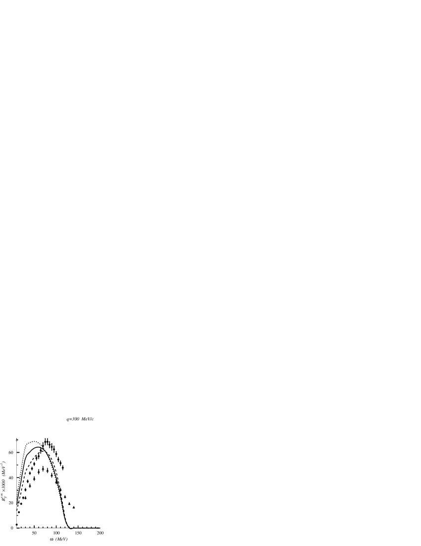
Figure 11: Mean field calculation for the transverse response on ${}^{40}Ca$ at different transferred momenta. Data from [2, 3] (circles) and from [7, 9] (triangles). Solid line: Mean field calculation with $m_{\rho}=600~{}MeV$; dashed line: mean field calculation with $m_{\rho}=770~{}MeV$; dotted line: FFG calculation.

Assuming as the most reliable data the one provided by [7, 9] the agreement between mean field and experiment is not completely satisfactory, but nevertheless less dramatic than in the case of Saclay data. It is clear how the assumption of an effective mass for the $\rho$ improves the agreement.

As an aside, without showing the figures for sake of brevity, we observe that Iron display the same trend as the Calcium.

6 The one-loop corrections

We finally come to the one-loop corrections, namely the ultimate goal of this paper.

First, let us define once forever the sets of parameters we shall use. We remark however that this same set of parameters is used in all the calculations presented in this paper.

1. The mass of the $\rho$-meson has been set to 600 $MeV$ in the spin-transverse channel, while in the scalar-isovector has been left unchanged ($m_{\rho}=770~{}MeV$)

2. The mass of the $\omega$ has been left unchanged too ($m_{\omega}=770~{}MeV$)

3. The pion coupling constant have been assumed, as usual, as $\frac{f^{2}_{\pi NN}}{4\pi}=0.08$, $\frac{f^{2}_{\pi N\Delta}}{4\pi}=0.32$ and $\frac{f^{2}_{\pi\Delta\Delta}}{4\pi}=0.016$. The last value comes from the quark model and is of course quite uncertain.

4. We assumed $C_{\rho NN}=C_{\rho N\Delta}=C_{\rho\Delta\Delta}=2.3$ in the spin-transverse channel and $=0.05$ in the scalar-isovector one. Further, $C_{\omega NN}=C_{\omega\Delta\Delta}=0.15$ in the scalar-isoscalar channel and $=1.5$ in the isoscalar spin-transverse one.

5. $g_{0}^{\prime}$ is set to 0.35.

6. The many-body cut-off of SRC are put to $q_{c,L}=800Mev/c$ and $q_{c,T}=1300Mev/c$.

7. The pion cut-off at the vertices are set to $\Lambda_{\pi NN}=1300Mev/c$, $\Lambda_{\pi N\Delta}=\Lambda_{\pi\Delta\Delta}=1000Mev/c$.

8. The $\rho NN$ cut-off at the vertex in the spin-transverse channel is $\Lambda_{\rho NN}=1750Mev/c$.

9. All the remaining cut-offs at the vertices are set to $1000Mev/c$.

The one-loop corrections to the response stem from many diagrams, corresponding to different physical effects. We start with the longitudinal response and we examine, as a guideline, the case of Carbon at a transferred momentum of $300~{}MeV/c$.

First let us examine the case of pure nucleon dynamics (no $\Delta$’s) and let us also drop the RPA dressing in the mean field (pure Lindhard function) as well as in the external legs of the one-loop corrections (this means that we examine only the contribution stemming from the black bubble of fig. 3, corresponding to the five diagrams of fig. 2). There are three contributions there, that we called self-energy, exchange and correlation terms. They correspond respectively to the first two diagrams of the first line of fig. 2, to the third diagram of the first line of fig. 2 and to the two diagrams of the second line of fig. 2. With the present choice of the parameters the main effects come from the isovector spin-longitudinal and spin-transverse channels, that turn out to be rather similar, while the other channels give a negligible contribution. In fig. 13 these one-loop corrections are shown, and clearly, while going in the right direction, are still not sufficient to explain the quenching of the peak. In passing we observe that exchange and correlation contribution display a trend opposite to the one of self-energy diagrams, thus corroborating our initial statement that in the loop expansion cancellations are realized order-by-order.

Figure 12: The one-loop corrections to the longitudinal response for ${}^{12}C$ without RPA dressing of the mean field and without $\Delta$’s. Dash-dotted line: FFG; dashed line: FFG plus self-energy diagrams; dotted line: FFG plus self-energy and exchange diagrams; solid line: FFG plus self-energy, exchange and correlation diagrams.

The next step is to introduce the $\Delta$-resonance. On physical grounds we expect that box diagrams will dominate the response. They are equivalent to the combination of the subdiagrams 4c) with 4a^′), 4a with 4c^′) and 4c with 4c^′) in fig. 6. They are shown in fig. 13 together with a complete calculation, i.e., with all possible diagrams. It appears that the box diagrams are dominant indeed and that they make the job the $\sigma$-meson is expected to do, namely to strongly enhance the peak. There is an important consideration to outline here, namely the fact that the peak is now softened.

Figure 13: The one-loop corrections to the longitudinal response for ${}^{12}C$ without RPA dressing of the mean field. Dash-dotted line: FFG; dashed line: diagrams without $\Delta$; dotted line: box diagrams only added; solid line: all diagrams.

Since in going to the complete treatment of the response we need the real part too of the diagrams, we show in fig. 14 the real part of the polarization propagator corresponding to the diagrams of fig. 13.

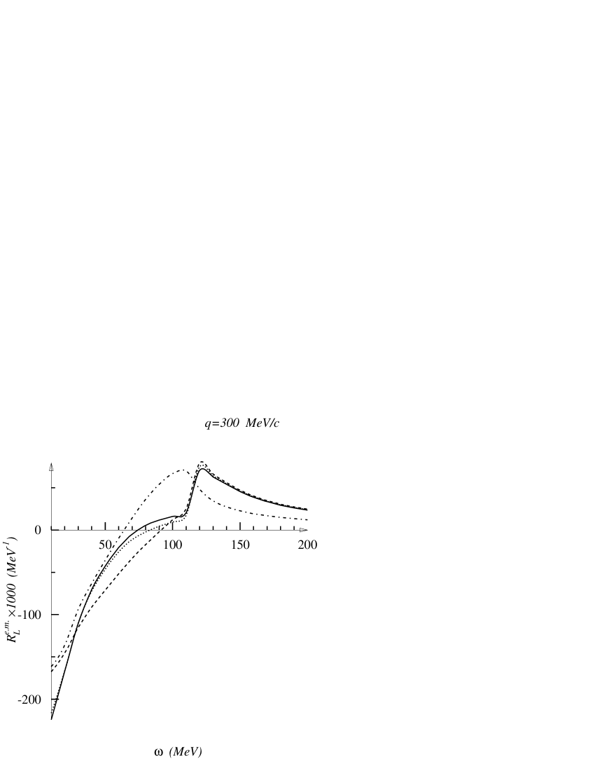
Figure 14: The one-loop corrections to the real part of the polarization propagator. Diagrams and lines as in fig. 13.

Finally in fig. 15 we plot the complete graph, with the inclusion of the RPA dressing everywhere.

Figure 15: The longitudinal response on ${}^{12}C$. Solid line: full response; dashed line: all diagrams without RPA; dotted line: diagrams without $\Delta$’s only but with RPA; dash-dotted line: mean field; dash-dotted-dotted line: FFG

From the figure it is clearly evident the compensation between two different effects - the hardening coming from the box diagram contributions and the softening deriving by RPA dressing at the mean field level: they correspond in a mean field description to the compensation between $\sigma$- and $\omega$-meson, as expected from Dirac phenomenology [41, 42, 43]. The final effect is to go back to the experimental data.

Next we examine the transverse response, following the same path as before.

Figure 16: The one-loop corrections to the spin-transverse response for ${}^{12}C$ without RPA dressing of the mean field and without $\Delta$’s. Dash-dotted line: FFG; dashed line: FFG plus self-energy diagrams; dotted line: FFG plus self-energy and exchange diagrams; solid line: FFG plus self-energy, exchange and correlation diagrams.

In fig. 16 the one-loop corrections are drawn, without RPA dressing of the mean field and without $\Delta$’s. The path is clearly similar to that of fig. 12 and is even more pronounced, but in the wrong direction, however. This can be understood in this way: the main effect, as both figures display, come from the self-energy diagrams, that deplete the peak, the only difference being a factor 2 which emphasizes the depletion in the transverse channel. Thus there is no way of reproducing the experimental data (that on the other hand are nicely described, up to a shift, by the simple FFG curve) without invoking other effects, as the $\Delta$ dynamics and the RPA-dressing effects.

Figure 17: The one-loop corrections to the spin-transverse response for ${}^{12}C$ without RPA dressing of the mean field. Dash-dotted line: FFG; dashed line: diagrams without $\Delta$; dotted line: box diagrams only added; solid line: all diagrams.

The contribution of the $\Delta$ diagrams to the transverse response is then shown in fig. 17, again without RPA-dressing. This time an important difference arises, concerning the contribution of the box diagrams, that are almost irrelevant. The origin of this seemingly contradictory behaviour stems from the spin traces, shown in table 7. It appears there that the spin traces for the case of a scalar probe and two spin-transverse particle exchanged are proportional to $1+\cos^{2}\theta_{pq}$ (see appendix B for notations) while for a spin-transverse probe the traces are proportional to $\pm\left(\frac{3}{2}-\frac{1}{2}\cos^{2}\theta_{kq}-\frac{1}{2}\cos^{2}\theta_{kp}-\frac{1}{2}\cos^{2}\theta_{pq}\right)$, thus ensuring large cancellation in the latter case, while in the former the two terms sum up together. In fig. 17 it is evident indeed that the box diagrams contribute very poorly to the response, but this time isospin selection rule does not forbid any of the remaining diagrams, which instead cancel almost completely the depletion induced by the self-energy diagrams. In conclusion the one-loop corrections are almost negligible in the transverse channel.

Finally in fig. 18 the whole calculation is reported.

Figure 18: The transverse response on ${}^{12}C$. Solid line: full response; dashed line: all diagrams without RPA; dotted line: diagrams without $\Delta$’s only but with RPA; dash-dotted line: mean field; dash-dotted-dotted line: FFG

Here the physical insight are clear: since one-loop corrections are negligible, we are now sensitive to the RPA-dressing of the $\rho$-meson channel (the dominant one): we require here an effective interaction near to vanish, in order to not further deplete the peak. The one we have chosen is still a little bit repulsive: clearly the momentum region between 300 and 400 MeV/c is the most sensitive to the details of the effective interaction. As a matter of fact our results stay more or less between Saclay’s and Jourdan’s data.

A more complete survey of our results for ${}^{12}C$ is presented in fig. 19 for the longitudinal and in fig. 20 for the transverse case.

Figure 19: Full calculation for the longitudinal response on ${}^{12}C$ at different transferred momenta. Data from [2, 3] (circles) and from [7, 9] (triangles). Solid line: full calculation; dashed line: Mean field calculation; dotted line: FFG calculation.

Figure 20: Full calculation for the transverse response on ${}^{12}C$ at different transferred momenta. Data from [2, 3] (circles) and from [7, 9] (triangles). Solid line: full calculation; dashed line: Mean field calculation; dotted line: FFG calculation.

The figures 21 and 22 present instead the results of our calculation ons ${}^{40}Ca$. In this case we have assumed an higher value for ${k_{F}}$, namely ${k_{F}}$=1.2 fm^-1, which better describes a medium nucleus. The interplay between RPA dressing of the external legs of the diagrams and the one-boson-loop corrections, which also alter the real part of the diagram (a density-dependent effect) leads to a more pronounced depletion of the longitudinal response, in agreement with the Saclay data. This results is relevant in our opinion and deserves a comment. First of all we stress once more that our approach is semi-phenomenological and that we have adjusted the free parameters of the model in such a way to agree with the Saclay data and other more refined experimental results are expected before to draw definite conclusions. For a long time the apparent discrepancy between the Saclay data on Carbon and Calcium, that provide so different Coulomb sum rule, led some people to question about the Calcium data. We have shown here that such a discrepancy may be explained as a density effect in the frame of a well defined theoretical model (the boson loop expansion), without violating the Coulomb sum rule. In fact it is clear from figs. 18 and 20 that the one-loop corrections are washed out when the transferred momentum increases and since the effective interaction in the spin-scalar channels is also vanishing at high $q$ then the mean field result also reduces in this limit to the FFG result: then the Coulomb sum rule is automatically fulfilled .

Figure 21: Full calculation for the longitudinal response on ${}^{40}Ca$ at different transferred momenta. Data from [2, 3] (circles) and from [7, 9] (triangles). Solid line: full calculation; dashed line: Mean field calculation; dotted line: FFG calculation.

Figure 22: Full calculation for the transverse response on ${}^{40}Ca$ at different transferred momenta. Data from [2, 3] (circles) and from [7, 9] (triangles). Solid line: full calculation; dashed line: Mean field calculation; dotted line: FFG calculation.

Still our results display a drawback. In the ${}^{40}Ca$ data ad low transferred momenta we have not displayed our results in the tail of the QEP. There an instability is already apparent in the ${}^{12}C$ data (where it could be regularized by interpolation procedure used in drawing the curves) and becomes more pronounced in Calcium. This could be unpleasant, but it is in our opinion consistent with our approach. The main difficulty of the boson loop expansion is that it is impossible at a given finite order in the number of loops to account for the shift of the QEP. This comes out in fact from the sum of the whole Dyson series in the fermionic lines of the particle-hole propagator, that in turn amounts to consider an infinite order in the loop expansion. The self-energy term in the one-boson loop correction tries to simulate the shift of the QEP by reshaping it, so that this diagram is particularly effective on the edges of the peak. On the other hand we know that our approach preserves all general theorems and sum rules (like, e.g., the $f^{\prime}$ sum rule) thus forcing, on the whole, a cancellation between different contributions, and in fact exchange and correlation terms have opposite sign with respect to the self-energy. The cancellation is ensured however at the level of the integrated response, while in the details some mismatches can survive were the corrections are more pronounced. Coherently with our approach this happens exactly where the one-boson-loop approximation must fail, i.e., on the edges of the QEP where its shift cannot be accounted for. Remarkably the RPA dressing of the external legs emphasizes the effect.

Finally, we want to discuss the discrepancies between Saclay and Jourdan data. These are particularly emphasized in the transverse response. Recalling our previous discussion, the Jourdan data seem to require a less pronounced attraction in the isovector spin-transverse effective interaction. Since we decreased in our calculations the $\rho$-mass just to emphasize the attractive part of the interaction we reproduce in fig. 23 our results both with $m_{\rho}$=770 MeV and with $m_{\rho}$=600 MeV. The figure seems to suggest that a value more or less in between the two we have displayed should better agree with the Jourdan data. Considering however that still the uncertainty in the experimental situation survives and that no microscopical calculations are presently available for the $\rho$-meson mass in the nuclear medium, further discussions on this topic are still premature.

Figure 23: Transverse response for ${}^{40}Ca$ with all diagrams with different $\rho$-masses. Solid line: $m_{\rho}=770$ MeV, dashed line: $m_{\rho}=600$ MeV.

7 Conclusions

Having presented in the previous section our numerical results we can now try to critically examine our approach and to draw some conclusions.

As emphasized in sect. 3 we changed somehow our philosophy during the completion of this program and ultimately we arrived to see our approach as an improvement upon the Landau-Migdal theory of nuclear matter.

As is well known, in fact, concerning the nuclear responses, the Landau-Migdal theory amounts to parametrize (usually with a constant) the effective interaction in a given channel and to explain the responses in terms of RPA, nothing but our mean field level.

The boson loop expansion first of all embodies the Landau-Migdal theory in a well behaved theoretical frame, thus opening the way to explore its microscopical content. In the present approach however we limited ourselves still to a semi-phenomenological theory by fitting the input in such a way to reproduce experimental outcome, but setting it at the one-loop order instead of at the mean field level.

The advantages of this procedure are physically relevant. As already explained the one-loop corrections are in fact sensitive to the momentum dependence of the effective interaction, while the mean field is not (at least up to a large extent). Furthermore degrees of freedom like $\Delta$-resonances can be explicitly handled in the internal lines, their contribution being relevant, as our results show.

Further, all sum rules are preserved at the one-loop order. In particular our results show that at sufficiently high $q$ (of the order of 600 MeV) no significant discrepancy from Coulomb sum rule is observed. $f^{\prime}$ sum rule is not examined here, but we will devote to it a future paper. As noted in ref. [1] however, with a poorer dynamical saturation of $f^{\prime}$ sum rule already occurred.

The phenomenological input of our model is represented by the effective particle-hole interactions. They follow, as far as possible, the standard schemes of meson-exchange models, but contain a parameter, stemming from many-body mechanisms, that fixes their range and is of central importance in ruling the size of the one-loop corrections. We have seen that the most relevant effective interaction, namely the isovector spin-transverse one, is also almost unknown. However, the one-loop corrections in this channels are so weak that the experimental data can be directly used to fix it.

The detailed analysis given above shows then a completely different dynamics in the longitudinal and transverse channels. The longitudinal channel is heavily affected by the $\sigma$-$\omega$ (the former being described by the box diagrams) interplay, that not only depletes, but also reshapes the peak, while the transverse one by one side is unaffected by $\sigma$ and $\omega$ exchange, and on the other displays major corrections coming from the direct $\Delta$-excitations, that tends to cancel all the one-loop effects.

It is obvious that the full determination of the effective interaction is a task that can be done only when the approximation scheme is given and that, in this sense, the present work could be seen as an essentially more complicated fit to the effective interaction itself. This is partly true, at least because we must redetermine the parameters at the 1-loop order. But the critical point is that this procedure could not be carried on at the mean field level, as it was shown in sect. 5, or, at least, it cannot be performed with reasonable choices for the parameters determining the effective interaction: this means, conversely, that the 1-loop corrections introduced into the calculation some non trivial and channel dependent momentum and/or energy dependences into the responses; these behaviours cannot be convincingly explained (or simulated) at the mean field level. We distinguish here two different regimes. First, we repeatedly stated that the most critical parameters are those ruling the medium/high momentum behaviour of the effective interaction, namely are $q_{c\,L}$ and $q_{c\,T}$, i.e., exactly those parameters which cannot be fixed at the mean field level. Secondly , the low momentum parts of the effective interaction is ruled by the Landau-Migdal parameters, and they are conceptually different at the mean field level and at 1-loop level. In the former case in fact they account also for the non-nucleonic dynamics, while in the latter the box diagrams have been disentagled from the Landau-Migdal parameters and explicitly accounted for. As a consequence the contrast between the value of the Landau-Migdal parameters and the corresponding microscopic interactions is dramatic at the mean field level, while is qualitatively weakened in going to the 1-loop level – an encouraging achievement.

In this context a seemingly disturbing feature is the value of $g^{\prime}(0)$, which turns out to be .35; we want to outline that a conventional value like $g^{\prime}(0)=g^{\prime}_{0}\simeq.7$ was primarily motivated by the need of preventing the unwanted and unobserved pion condensation: this requirement truly fixes a lower bound on $g^{\prime}(q\simeq 2k_{F})$, which coincides with $g^{\prime}_{0}$ only in the pure Landau-Migdal theory. In our momentum dependent description of $g^{\prime}_{L}$ we obtain, in fact, $g^{\prime}(q\simeq 2k_{F})\simeq 0.7$.

Having so characterized our approach it is now clear why we have adapted our parameters on the Saclay’s results: simply it was the only complete set of data available. When the transverse response from Bates will become available too, the same procedure can be repeated and reasonably a different effective interaction could be found able to explain these data. Clearly this possibility does not alter our theoretical frame. Needless to say, the physical information will change, because ultimately we can interpret the search for the parameters of our model as a way to get information about the effective interactions. Thus we complain once more the present ambiguities of the experimental data, because it precludes the possibility of attributing a safe physical meaning to the effective interaction derived in this work. To further exemplify this topic, let us remind that while Saclay data seem to suggest an in-medium-mass for the $\rho$-meson around 600 $MeV$, the analyses of Jourdan are more compatible with a somehow higher $\rho$-mass. Again this outcome stresses the relevance of a reliable set of experimental data.

To conclude this paper, we also want to outline the persisting weaknesses of our approach. It is apparent in fact that the transverse response comes out to be too large with respect to experimental data and, if one looks carefully, the same seems to be true for the longitudinal one at high transferred momentum. Furthermore the $q$-dependence of the corrections could be somehow overemphasized, as they seems to be more pronounced at low $q$’s and to fade out too quickly (not dramatically, however). This last topic suggests a careful analysis of the nuclear densities we have chosen. In fact, for dimensional reasons, the fading out of the corrections is expected to vary with $k_{F}/q$ and a lower value of $k_{F}$ could both narrow the peak and spread over a larger range the fading of the 1-loop corrections.

We used in this paper $k_{F}=1.1fm^{-1}$ for ${}^{12}C$ and $k_{F}=1.2fm^{-1}$ for ${}^{40}Ca$, very traditional figures for the Fermi momentum of medium/light nuclei. They come however from old analyses carried out at rather low momenta. Many accidents could make this choice questionable: the relativistic kinematics first of all, and then the need in light nuclei of a local density approach (equivalent in some sense to a lower average density) an so on. Last but least the effect of the $\Delta$ tail in the QEP region should also be accounted for before extracting from QEP a phenomenological value for $k_{F}$.

All these considerations suggest, before going on with an improved dynamics (we mean at least energy-dependent meson propagators), to carefully re-examine the responses in the region where, as our calculations show, the FFG is quite sufficient to explain the data, i.e, above – roughly – 600 $MeV/c$. Thus a non-trivial task, to be pursued in a near future, should be a careful re-derivation of the FFG parameters in the relativistic regime. In these conditions it is known [47] that the nuclear and nucleon physics are inextricably linked. Curiously enough, the solution of this last problem becomes a fundamental input for the models that should explain the dynamics at lower energy and momentum domains.

Appendix A The matrices $\cal S$

The matrices $\cal S$ are defined as

$${\cal S}_{1}=\left(\matrix{0&\sqrt{3}&0&0\cr\sqrt{3}&0&2&0\cr 0&2&0&\sqrt{3}\cr 0&0&\sqrt{3}&0}\right)\qquad{\cal S}_{2}=\left(\matrix{0&-i\sqrt{3}&0&0\cr i\sqrt{3}&0&-2i&0\cr 0&2i0&-i\sqrt{3}\cr 0&0&i\sqrt{3}&0}\right)$$

$${\cal S}_{3}=\left(\matrix{3&0&0&0\cr 0&1&0&0\cr 0&0&-1&0\cr 0&0&0&-3}\right)$$ (21)

The traces we need are listed below:

$${\rm Tr}(\sigma_{i}\sigma_{j}) = 2\delta_{ij}$$ (22)

$${\rm Tr}(\sigma_{i}\sigma_{j}\sigma_{k}) = 2i\epsilon_{ijk}$$ (23)

$${\rm Tr}(\sigma_{i}\sigma_{j}\sigma_{k}\sigma_{l} = 2(\delta_{ij}\delta_{kl}-\delta_{ik}\delta{jl}+\delta_{il}\delta_{jk})$$ (24)

$${\rm Tr}(S^{\dagger}_{i}S_{j}) = \frac{4}{3}\delta_{ij}$$ (25)

$${\rm Tr}(S^{\dagger}_{i}S_{j}\sigma_{k}) = -\frac{2}{3}i\epsilon_{ijk}$$ (26)

$${\rm Tr}(S^{\dagger}_{i}{\cal S}_{j}S_{k}) = \frac{10}{3}i\epsilon_{ijk}$$ (27)

$${\rm Tr}(\sigma_{i}\sigma_{j}S^{\dagger}_{k}S_{l}) = \frac{4}{3}\delta_{ij}\delta_{kl}+\frac{2}{3}\delta_{ik}\delta{jl}-\frac{2}{3}\delta_{il}\delta_{jk}$$ (28)

$${\rm Tr}(S^{\dagger}_{i}S_{j}S^{\dagger}_{k}S_{l}) = \frac{8}{9}\delta_{ij}\delta_{kl}-\frac{2}{9}\delta_{ik}\delta{jl}+\frac{2}{9}\delta_{il}\delta_{jk}$$ (29)

$${\rm Tr}(S^{\dagger}_{i}{\cal S}_{j}S_{k}\sigma_{l}) = -\frac{2}{3}\delta_{ij}\delta_{kl}+\frac{8}{3}\delta_{ik}\delta{jl}-\frac{2}{3}\delta_{il}\delta_{jk}$$ (30)

$${\rm Tr}(S^{\dagger}_{i}{\cal S}_{j}{\cal S}_{k}S_{l}) = -\frac{2}{3}\delta_{ij}\delta_{kl}-\frac{22}{3}\delta_{ik}\delta{jl}+\frac{28}{3}\delta_{il}\delta_{jk}$$ (31)

Appendix B Evaluation of the traces

The traces of the diagrams are composed by a spin and an isospin part. Further, we must examine the diagrams 1, 3 and 4 (the traces of the diagrams 2 and 5 are equal to those of 1 and 4). To fix the kinematic, we denote with $\bf k$ the momentum of the probe, and with $\bf q$ the integrated momentum flowing through the bosonic loop and with $\bf p$ the sum ${\bf p}={\bf k}+{\bf q}$. Further, we denote with $\theta_{xy}$ the angles between the vectors $\bf x$ and $\bf y$. The spin structure of the vertices is assumed to be $1$ for a scalar interaction, ${\mbox{\boldmath$\hat{h}$}}\cdot{\mbox{\boldmath$\sigma$}}$ for a spin-longitudinal interaction and ${\mbox{\boldmath$\hat{h}$}}\times{\mbox{\boldmath$\sigma$}}$ for a spin-transverse interaction, $\bf h$ being the momentum entering the vertex.

B.1 Diagrams 1 and 2

B.1.1 Isospin part

The coefficient are resumed in the table 1. The first column labels the diagrams as in fig. 4. SS denotes isoscalar probe and isoscalar interaction, SV denotes isoscalar probe and isovector interaction, VS denotes isovector probe and isoscalar interaction, VV denotes isovector probe and and isovector interaction.

SS SV VS VV a 2 6 2 6 b 0 0 4/3 4 c 0 4 0 4 d 0 0 0 8/3 e 0 0 0 4/3 f 0 0 0 4/3 g 0 4 0 20

Table 1: Isospin coefficients of the diagrams of fig. 4

B.1.2 Spin part

For the spin part the coefficients are given in table 2. Their analytic structure is $\alpha+\beta\cos^{2}\theta_{kq}$ Diagrams are labelled as in table 1. On the top row the first letter characterizes the probe and the second the interaction, with the convention: S = scalar channel, L = spin-longitudinal channel, T = spin-transverse channel. In each entry the quantity $\alpha$ is reported. If $\beta$ is non-vanishing, it is also reported after a semicolon. Finally, the in the spin-transverse channel the trace is taken only over the spin part of the diagram and not on its spatial part, which still keeps the form $\delta_{ij}-k_{i}k_{j}/k^{2}$. The spatial traces then carry an extra factor 2.

SS SL ST LS LL LT TS TL TT a 2 2 4 2 2 4 2 2 4 b 0 0 0 4/3 4/3 8/3 4/3 4/3 8/3 c 0 4/3 8/3 0 4/3 8/3 0 4/3 8/3 d 0 0 0 0 8/9 16/9 0 8/9 16/9 e 0 0 0 0 2/9;2/3 10/9;-2/3 0 5/9;-1/3 7/9;1/3 f 0 0 0 4/3 28/3;-8 32/3;8 4/3 16/3;4 44/3;-4 g 0 4/3 8/3 0 28/3;-8 32/3;8 0 16/3;4 44/3;-4

Table 2: Spin coefficients of the diagrams of fig. 4

B.2 Diagram 3

The spin and isospin parts of the traces have the same structure as for the diagrams 1 and 2. The isospin coefficients are listed in table 3 while the spin coefficients are listed in table 4.

SS SV VS VV a 2 6 2 -2 b,c,d,e 0 0 0 8/3 f,j 0 0 4/3 20/3 g,i 0 0 0 4/9 h,k 0 4 0 20/3 l,m,n,o 0 0 0 -40/3

Table 3: Isospin coefficients of the diagrams of fig. 5

SS SL ST LS LL LT TS TL TT a 2 2 4 2 -2;4 0;-4 2 0;-2 -2;2 b,c,d,e 0 0 0 0 2/3;2/3 2;-2/3 0 1;-1/3 5/3;1/3 f,j 0 0 0 1/3 5/3;-1/3 4;4/3 4/3 2;2/3 14/3;-2/3 g,i 0 0 0 0 -2/9;10/9 2/3;-10/9 0 1/3;-5/9 1/9;5/9 h,k 0 4/3 8/3 0 5/3;-1/3 4;4/3 0 2;2/3 14/3;-2/3 l,m,n,o 0 0 0 0 -22/3;26/3 -6;-26/3 0 -3;-13/3 -31/3;13/3 g 0 4/3 8/3 0 28/3;-8 32/3;8 0 16/3;4 44/3;-4

Table 4: Spin coefficients of the diagrams of fig. 5

B.3 Diagrams 4 and 5

In these diagrams spin-isospin traces have 3 components. As fig. 6 clearly explain, the diagrams are obtained by connecting two fermionic loops (in this subsection we shall call them subdiagrams): we have to take the spin-isospin traces of the two subdiagrams, that depend upon the spin-isospin character of the probe and of the exchanged particles (first two factors), the traces however may generate two tensor in the isospin or configuration space, to be then saturated together, thus giving rise to the third factor (we shall call it “connecting factor”).

The spin-isospin traces of the subdiagrams depend only upon the scalar or vector character of the probe and of the exchanged particles as far as the numerical coefficient is concerned, and amount to evaluate the traces of two or three generalized Pauli matrices, listed in appendix A. The difference between spin-longitudinal and spin-transverse channel instead only affects the connecting factor. Thus in table 3 we give the numerical coefficients in the various cases.

a b c d e f g SSS 2 0 0 0 0 0 0 SVV 2 0 4/3 0 0 4/3 0 VVS 2 4/3 0 0 0 0 4/3 VSV 2 0 0 4/3 4/3 0 0 VVV 2 -2/3 -2/3 /-2/3 10/3 10/3 10/3

Table 5: Numerical coefficient of the traces of the subdiagrams of diagrams 4 and 5. In the first column the scalar (S) or vector (V) character of the probe, the first (upper) and second (lower) exchanged particle are reported in the given order. The channels not reported here have vanishing coefficients.

The spin-isospin traces are thus obtained by multiplying the entries of table 5 corresponding to the required subdiagrams by the connecting factors given in table 7 for the isospin and in table 7 for the spin. The tensors arising from the spatial part of the traces are also listed.

probe upper part. lower part. tensor coeff. S S S I 1 S S V 0 S V S 0 S V V $\delta_{ij}$ 3 V S S 0 V S V $\delta_{i3}$ 1 V V S $\delta_{i3}$ 1 V V V $i\epsilon_{ij3}$ $\mp 2$

Table 6: Connecting coefficients of the isospin traces.

probe upper part. lower part. tensor S S S 1 1 0 0 0 S S L 0 0 0 0 0 S S T 0 0 0 0 0 S L S 0 0 0 0 0 S L L $\delta_{ij}p_{i}q_{j}\delta_{kl}p_{k}q_{l}$ 0 0 0 1 S L T $\delta_{ij}p_{i}\delta_{kl}p_{k}\tilde{q}_{jl}$ 1 0 0 -1 S T S 0 0 0 0 0 S T L $\delta_{ij}q_{j}\delta_{kl}q_{l}\tilde{p}_{ik}$ 1 0 0 -1 S T T $\delta_{ij}\delta_{kl}\tilde{p}_{ik}\tilde{q}_{jl}$ 1 0 0 1 L S S 0 0 0 0 0 L S L $\delta_{ij}k_{i}q_{j}\delta_{kl}k_{k}q_{l}$ 0 1 0 0 L S T $\delta_{ij}k_{i}\delta_{kl}k_{k}\tilde{q}_{jl}$ 1 -1 0 0 L L S $\delta_{ij}k_{i}p_{j}\delta_{kl}k_{k}p_{l}$ 0 0 1 0 L L L $i\epsilon_{ijk}k_{i}p_{j}q_{k}i\epsilon_{lmn}k_{l}p_{m}q_{n}$ 0 0 0 0 L L T $i\epsilon_{ijk}k_{i}p_{j}i\epsilon_{lmn}k_{l}p_{m}\tilde{q}_{kn}$ $\mp 1$ 0 $\pm 1$ 0 L T S $\delta_{ij}k_{i}\delta_{kl}k_{k}\tilde{p}_{jl}$ 1 0 -1 0 L T L $i\epsilon_{ijk}k_{i}q_{k}i\epsilon_{lmn}k_{l}q_{n}\tilde{p}_{jm}$ $\mp 1$ $\pm 1$ 0 0 L T T $i\epsilon_{ijk}k_{i}i\epsilon_{lmn}k_{l}\tilde{p}_{jm}\tilde{q}_{ln}$ 0 $\mp 1$ $\mp 1$ 0 T S S 0 0 0 0 0 T S L $\delta_{ij}q_{j}\delta_{kl}q_{l}\frac{1}{2}\tilde{k}_{ik}$ $\frac{1}{2}$ $-\frac{1}{2}$ 0 0 T S T $\delta_{ij}\delta_{kl}\frac{1}{2}\tilde{k}_{ik}\tilde{q}_{jl}$ $\frac{1}{2}$ $\frac{1}{2}$ 0 0 T L S $\delta_{ij}p_{j}\delta_{kl}p_{l}\frac{1}{2}\tilde{k}_{ik}$ $\frac{1}{2}$ 0 $-\frac{1}{2}$ 0 T L L $i\epsilon_{ijk}p_{j}q_{k}i\epsilon_{lmn}p_{l}q_{n}\frac{1}{2}\tilde{k}_{ik}$ $\mp\frac{1}{2}$ 0 0 $\pm\frac{1}{2}$ T L T $i\epsilon_{ijk}p_{j}i\epsilon_{lmn}p_{m}\frac{1}{2}\tilde{k}_{ik}\tilde{q}_{kn}$ 0 0 $\mp\frac{1}{2}$ $\mp\frac{1}{2}$ T T S $\delta_{ij}\delta_{kl}\frac{1}{2}\tilde{k}_{ik}\tilde{p}_{jl}$ $\pm\frac{1}{2}$ 0 $\pm\frac{1}{2}$ 0 T T L $i\epsilon_{ijk}q_{k}i\epsilon_{lmn}q_{n}\frac{1}{2}\tilde{k}_{il}\tilde{p}_{jm}$ 0 $\mp\frac{1}{2}$ 0 $\mp\frac{1}{2}$ T T T $i\epsilon_{ijk}i\epsilon_{lmn}\frac{1}{2}\tilde{k}_{il}\tilde{p}_{jm}\tilde{q}_{kn}$ $\mp\frac{3}{2}$ $\pm\frac{1}{2}$ $\pm\frac{1}{2}$ $\pm\frac{1}{2}$

Table 7: Connecting factors of the spatial traces. S, L and T refer respectively to scalar, spin-longitudinal and spin-transverse particles. The $\pm$ sign, when occurs, refers to diagram 4 (upper sign) and 5 (lower sign). The four last entries are respectively the constant term, the coefficient of $\cos^{2}\theta_{kq}$, $\cos^{2}\theta_{kp}$ and $\cos^{2}\theta_{pq}$.

References

- [1] R. Cenni and P. Saracco. Phys. Rev., C50:1851, 1994.
- [2] Z. E. Meziani et al. Phys. Rev. Lett., 52:2180, 1984.
- [3] Z. E. Meziani et al. Phys. Rev. Lett., 54:1233, 1985.
- [4] S. Boffi, C. Giusti and F. D. Pacati. Phys. Rep., 226C:1, 1993.
- [5] A. Zghiche et al. Nucl. Phys., A572:513, 1994.
- [6] T. C. Yates et. al. Phys. Lett., 312B:382, 1993.
- [7] J. Jourdan. Phys. Lett., B353:189, 1995.
- [8] M. B. Barbaro et al. Nucl. Phys., B569:701, 1994.
- [9] J. Jourdan. Nucl. Phys., A603:117, 1996.
- [10] S. Fantoni and V. R. Pandharipande. Nucl. Phys., A473:234, 1987.
- [11] G. P. Cò, K. F. Quader, R. D. Smith and J. Wambach. Nucl. Phys., A485:61, 1988.
- [12] M. Barbaro et al. To be published on Nucl. Phys. A.
- [13] V. Van der Sluys, J. Rickebusch and M. Waroquier. To be published on Phys. Rev. C.
- [14] W. M. Alberico, M. Ericson and A. Molinari. Ann. Phys., 154:356, 1984.
- [15] J. E. Amaro, G. Cò and A. M. Lallena. Nucl. Phys., A578:365, 1994.
- [16] R. Cenni and S. Fantoni. Phys. Lett., B314:260, 1993.
- [17] T. S. Walhout, R. Cenni, A. Fabrocini and S. Fantoni. Phys. Rev., C54:1622, 1996.
- [18] A. Fabrocini. ”To be published on the proceedings of the “Workshop on electron nucleus scattering” - Marciana Marina, Elba, July 1-5 1996”.
- [19] R. Cenni, F. Conte and P. Saracco. J. Phys. G, 22:L71, 1996.
- [20] W. M. Alberico, R. Cenni, A. Molinari and P. Saracco. Ann. of Phys., 174:131, 1987.
- [21] R. Cenni. volume 6 of Condensed Matter Theories. Plenum Press, New York and London, 1990. Edited by S. Fantoni and S. Rosati.
- [22] W. M. Alberico, R. Cenni, A. Molinari and P. Saracco. Phys. Rev., C38:2389, 1988.
- [23] R. Cenni and P. Saracco. Nucl. Phys., A487:279, 1988.
- [24] R. Cenni, F. Conte, A. Cornacchia and P. Saracco. La Rivista del Nuovo Cimento, 15 n. 12, 1992.
- [25] W. M. Alberico, R. Cenni, A. Molinari and P. Saracco. Phys. Rev. Lett., 65:1845, 1990.
- [26] G. Morandi, E. Galleani d’Agliano, F. Napoli and C. Ratto. Adv. Phys., 23:867, 1974.
- [27] H. Keiter. Phys. Rev., 2B:3777, 1970.
- [28] H. Kleinert. Fort. Phys., 26:565, 1978.
- [29] J. Speth, E. Werner and J. Wild. Phys. Rep., 33:127, 1977.
- [30] R. Cenni. In J. Arvieux and E. De Sanctis, editor, The ELFE project: an Electron Laboratory for Europe p. 437 – Mainz, October 1992, page 437, 1993.
- [31] R. Machleidt, K. Holinde and Ch. Elster. Phys. Rep., C149:1, 1987.
- [32] E. Oset G. E. Brown, S. O. Bäckman and W. Weise. Nucl. Phys., A286:191, 1977.
- [33] E. Oset and L. L. Salcedo. Nucl. Phys., A468:631, 1987.
- [34] E. Oset and W. Weise. Nucl. Phys., A319:365, 1979.
- [35] E. Oset and W. Weise. Nucl. Phys., A329:47, 1979.
- [36] G. E. Brown and W. Weise. Phys. Rep., C22:281, 1975.
- [37] T. De Forest, jr. Nucl. Phys., A414:347, 1984.
- [38] M. M. Giannini. Rep. Prog. Phys., 54:453, 1990.
- [39] M. Ericson and M. Rosa-Clot. Zeit. Phys., A324:373, 1986.
- [40] W. M. Alberico, R. Cenni, and A. Molinari. Prog. in Part. and Nucl. Phys., 23:171, 1989.
- [41] J. D. Walecka. Ann. Phys., 83:491, 1974.
- [42] B. C. Clark, S. Hama and R. L. Mercer. In H. O. Meyer, editor, The Interaction Between Medium Energy Nucleons in Nuclei, page 260. AIP Conference Proceedings, 1982.
- [43] B. C. Clark. In M. B. Johnson and A. Picklesimer, editor, Relativistic Dynamics and Quark-Nuclear Physics, page 302, New York, 1986. J. Wiley & Sons.
- [44] K. Holinde. Phys. Rep., C68:121, 1981.
- [45] D. B. Day, J. S. McCarthy, T. W. Donnelly and I. Sick. Ann. Rev. Nucl. Part. Sci., 40:357, 1990.
- [46] R. C. Carrasco and E. Oset. Nucl. Phys., A536:445, 1992.
- [47] R. Cenni, T. W. Donnelly and A. Molinari. Submitted to Phys. Rev. C.