Electroproduction of $\phi$ meson from proton
and the strangeness in the nucleon

Abstract

We analyze the process $e\,p\to e\,p\,\phi$ near the threshold within $uud$-$s\bar{s}$ cluster model as a probe of the strangeness content of proton. Our consideration is based on the relativistic harmonic oscillator quark model which takes into account the Lorentz-contraction effect of the hadron wavefunctions. We find that the knockout mechanisms are comparable to the diffractive production of vector-meson-dominance model when only (3–5)% strange quark admixture is assumed, which should be compared with (10–20)% of the nonrelativistic quark model prediction. The cross sections of the $uud$- and $s\bar{s}$-knockout processes have qualitatively different dependence on the four-momentum transfer squared to the proton and may be distinguished experimentally. We also briefly discuss a way to determine the strangeness content of proton in 5-quark cluster model.

I Introduction

Conventional phenomenological quark models widely used for describing low-energy properties of baryons treat nucleon as consisting of only up and down quarks; intrinsically, there is no strange quark in the nucleon. Considering the success of the constituent quark models [1], it may come as a surprise when some recent measurements and theoretical analyses indicate a possible existence of a significant strange quark content in the nucleon.

For example, analyses of the sigma term [2] in pion-nucleon scattering suggest that about one third of the rest mass of the proton comes from $s\bar{s}$ pairs inside the proton. The EMC measurement of the proton spin structure functions in deep-inelastic muon scattering [3, 4] has been interpreted as an indication of the strange quark sea $s\bar{s}$ strongly polarized opposite to the nucleon spin, leading to the conclusion that the total quark spin contributes little to the total spin of the proton. A similar conclusion has been drawn from the BNL elastic neutrino-proton scattering [5, 6]. This has stimulated a set of new experimental proposals [8] to measure the neutral weak form factors of the nucleon which might be sensitive to the strange quarks of the nucleon.

One of the intriguing idea associated with a direct probe of the strangeness content of proton is to use $\phi$ meson production from proton [9, 10, 11, 12]. Since $\phi$ meson is nearly 100% $s\bar{s}$-state because of the $\omega$-$\phi$ ideal mixing, its coupling to the proton is suppressed by the OZI rule. The main idea of this proposal, called OZI “evasion” process, is to determine the amount of the $s\bar{s}$-admixture of nucleon, if any, by isolating its contribution in $\phi$ production processes. For example, $s\bar{s}$ admixture in the proton wavefunction allows contributions from “shakeout” and “rearrangement” diagrams in $\phi$ production from $p\bar{p}$ and $pp$ collisions [12]. Another idea is to use $\phi$-meson lepto- and electroproduction from proton target as advocated by Henley et al. [9, 10]. In this case, in addition to the diffractive production mechanism of the vector-meson–dominance model (VDM) we have contributions from the direct “knockout” mechanism.

If we consider $s\bar{s}$ admixture of proton, we can parameterize the Fock-space decomposition of the proton wavefunction as

$$|p\rangle=A_{0}|uud\rangle+\sum_{X}A_{X}|uudX\rangle+\sum_{X}B_{X}|uuds\bar{s}X\rangle,$$ (1)

where $X$ denotes any combination of gluons and light quark pairs of $u$ and $d$ quarks. Analyses of the $\phi$ production experiments can give estimates on $B_{X}$. For instance, investigation of $p\bar{p}$ annihilation by connected quark line diagrams estimates that the $s\bar{s}$ sea quark contribution to the proton wavefunction is between 1% and 19% [13]. In Ref. [10], by using the $\phi$ electroproduction its upper bound is estimated to be about 10-20%. To obtain this estimation, the authors used nonrelativistic quark model (NRQM) and calculated the cross section of the $s\bar{s}$-knockout process. Because of the paucity of experimental data [14, 15], it was compared with the VDM predictions. However, as was pointed out by our previous publication [17] where a preliminary result was reported, the knockout contributions are closely related to the hadron form factors and in the considered kinematical region of $\phi$ production, the minimum value of $\mathchoice{{\hbox{\boldmath$\displaystyle q$}}}{{\hbox{\boldmath$\textstyle q$}}}{{\hbox{\boldmath$\scriptstyle q$}}}{{\hbox{\boldmath$\scriptscriptstyle q$}}}^{2}$ is about 3.6 GeV², where $\textstyle q$ is the three-momentum transferred to the hadron system. So it is clear that the value of the momentum transfer in this process is too large to use the NRQM because its predictions on hadron form factors are in poor agreement with experiment at $\mathchoice{{\hbox{\boldmath$\displaystyle q$}}}{{\hbox{\boldmath$\textstyle q$}}}{{\hbox{\boldmath$\scriptstyle q$}}}{{\hbox{\boldmath$\scriptscriptstyle q$}}}^{2}\geq 0.3$ GeV².

In this paper, we improve the work of Ref. [10] by including relativistic effects based on the relativistic harmonic oscillator model (RHOM) [18, 19, 20, 21, 22, 23, 24] which describes successfully the proton form factors in a wide range of $\mathchoice{{\hbox{\boldmath$\displaystyle q$}}}{{\hbox{\boldmath$\textstyle q$}}}{{\hbox{\boldmath$\scriptstyle q$}}}{{\hbox{\boldmath$\scriptscriptstyle q$}}}^{2}$. We also carry out the calculations for the $uud$-knockout and its interference with the $s\bar{s}$-knockout which were argued to be suppressed and left out in Ref. [10] as well as for the $s\bar{s}$-knockout. The calculations are done both in NRQM and in RHOM for a comparison. As in Ref. [10], we will compare the cross sections of the knockout processes with the VDM predictions. However, this does not mean that the knockout mechanism should replace the VDM mechanism. The latter is present as a background of the knockout mechanism and our purpose is to determine a theoretical upper bound of $B_{X}^{2}$ using $\phi$ electroproduction process.

This paper is organized as follows. In the next section, we briefly review the general structure of the knockout and VDM differential cross sections and introduce the kinematical variables for $\phi$ meson electroproduction. Then in Sect. III we discuss the proton wavefunction of 5-quark cluster model. Section IV is devoted to the evaluation of the knockout process matrix elements within the non-relativistic harmonic oscillator quark model. In Sect. V we perform the calculations based on the RHOM which provides an explanation of the dipole-like $Q^{2}$ dependence of the elastic nucleon form factor. This model, though probably it has not underlying physical significance, has the pleasant feature that basically all quantities of interest can be worked out analytically, and, in many cases, it allows understanding of the qualitative picture of the reaction. The nontrivial role of the relativistic Lorentz-contraction effect is also discussed. In Sec. VI we briefly discuss a way to extract out the strangeness content of proton in an extended quark model. Section VII contains a summary and some details in the calculation are given in Appendix.

II Kinematics and cross sections

The one-photon exchange diagram for $\phi$ electroproduction is shown in Fig. 1. The four momenta of the initial electron and proton, final electron and proton, the produced $\phi$ meson, and the virtual photon are denoted by $k$, $p$, $k^{\prime}$, $p^{\prime}$, $q_{\phi}$, and $q$, respectively. In the laboratory frame, we write $k\equiv(E_{e},\mathchoice{{\hbox{\boldmath$\displaystyle k$}}}{{\hbox{\boldmath$\textstyle k$}}}{{\hbox{\boldmath$\scriptstyle k$}}}{{\hbox{\boldmath$\scriptscriptstyle k$}}})$, $k^{\prime}\equiv(E_{e}^{\prime},\mathchoice{{\hbox{\boldmath$\displaystyle k$}}}{{\hbox{\boldmath$\textstyle k$}}}{{\hbox{\boldmath$\scriptstyle k$}}}{{\hbox{\boldmath$\scriptscriptstyle k$}}}^{\prime})$, $p\equiv(E_{p},\mathchoice{{\hbox{\boldmath$\displaystyle p$}}}{{\hbox{\boldmath$\textstyle p$}}}{{\hbox{\boldmath$\scriptstyle p$}}}{{\hbox{\boldmath$\scriptscriptstyle p$}}})=(M_{N},\mathchoice{{\hbox{\boldmath$\displaystyle 0$}}}{{\hbox{\boldmath$\textstyle 0$}}}{{\hbox{\boldmath$\scriptstyle 0$}}}{{\hbox{\boldmath$\scriptscriptstyle 0$}}})$, where $M_{N}$ is the nucleon mass, $p^{\prime}\equiv(E_{p}^{\prime},\mathchoice{{\hbox{\boldmath$\displaystyle p$}}}{{\hbox{\boldmath$\textstyle p$}}}{{\hbox{\boldmath$\scriptstyle p$}}}{{\hbox{\boldmath$\scriptscriptstyle p$}}}^{\prime})$, $q_{\phi}\equiv(\omega_{\phi},\mathchoice{{\hbox{\boldmath$\displaystyle q$}}}{{\hbox{\boldmath$\textstyle q$}}}{{\hbox{\boldmath$\scriptstyle q$}}}{{\hbox{\boldmath$\scriptscriptstyle q$}}}_{\phi})$, and $q\equiv(\nu,\mathchoice{{\hbox{\boldmath$\displaystyle q$}}}{{\hbox{\boldmath$\textstyle q$}}}{{\hbox{\boldmath$\scriptstyle q$}}}{{\hbox{\boldmath$\scriptscriptstyle q$}}})$, respectively. The electron scattering angle $\theta$ is defined by $\cos\theta=\mathchoice{{\hbox{\boldmath$\displaystyle k$}}}{{\hbox{\boldmath$\textstyle k$}}}{{\hbox{\boldmath$\scriptstyle k$}}}{{\hbox{\boldmath$\scriptscriptstyle k$}}}\cdot\mathchoice{{\hbox{\boldmath$\displaystyle k$}}}{{\hbox{\boldmath$\textstyle k$}}}{{\hbox{\boldmath$\scriptstyle k$}}}{{\hbox{\boldmath$\scriptscriptstyle k$}}}^{\prime}/\left|\mathchoice{{\hbox{\boldmath$\displaystyle k$}}}{{\hbox{\boldmath$\textstyle k$}}}{{\hbox{\boldmath$\scriptstyle k$}}}{{\hbox{\boldmath$\scriptscriptstyle k$}}}\right|\left|\mathchoice{{\hbox{\boldmath$\displaystyle k$}}}{{\hbox{\boldmath$\textstyle k$}}}{{\hbox{\boldmath$\scriptstyle k$}}}{{\hbox{\boldmath$\scriptscriptstyle k$}}}^{\prime}\right|$. We also denote the electron mass and $\phi$ mass by $M_{e}$ and $M_{\phi}$, respectively. The other invariant kinematical variables are $\nu\equiv p\cdot q/M_{N}=E_{e}-E_{e}^{\prime}$, the minus of photon mass squared $Q^{2}\equiv-q^{2}$, the four-momentum transfer squared to the proton $t\equiv(p-p^{\prime})^{2}$, the proton–virtual-photon center-of-mass energy $W^{2}=(p+q)^{2}$, and the total energy squared in the CM system $s=(p+k)^{2}$. We also use dimensionless invariant variables $\eta$, $y$ and $z$ defined as

$$\eta=\frac{Q^{2}}{4M_{N}^{2}},\quad y=\frac{-t}{4M_{N}^{2}},\quad z=\frac{W^{2}-M_{N}^{2}}{4M_{N}^{2}}.$$ (2)

So, in the laboratory frame we have

$$\mathchoice{{\hbox{\boldmath$\displaystyle q$}}}{{\hbox{\boldmath$\textstyle q$}}}{{\hbox{\boldmath$\scriptstyle q$}}}{{\hbox{\boldmath$\scriptscriptstyle q$}}}^{2}=4M_{N}^{2}[(\eta+z)^{2}+\eta],\quad\nu=2M_{N}(\eta+z),$$ (3)

$$E_{p}^{\prime}=M_{N}+2M_{N}y,\quad\omega_{\phi}=\nu-2M_{N}y,\quad s\simeq M_{N}(2E_{e}+M_{N}).$$ (4)

In terms of the conventional $T$-matrix elements $T_{fi}$, the differential cross section is given as

$${\rm d}\sigma_{fi}=(2\pi)^{4}\delta(p+q-p^{\prime}-q_{\phi})\frac{2E_{p}E_{e}}{\sqrt{\lambda(s,M_{e}^{2},M_{N}^{2})}}{\overline{|T_{fi}|^{2}}}\frac{{\rm d}\mathchoice{{\hbox{\boldmath$\displaystyle k$}}}{{\hbox{\boldmath$\textstyle k$}}}{{\hbox{\boldmath$\scriptstyle k$}}}{{\hbox{\boldmath$\scriptscriptstyle k$}}}^{\prime}}{(2\pi)^{3}}\frac{{\rm d}\mathchoice{{\hbox{\boldmath$\displaystyle p$}}}{{\hbox{\boldmath$\textstyle p$}}}{{\hbox{\boldmath$\scriptstyle p$}}}{{\hbox{\boldmath$\scriptscriptstyle p$}}}^{\prime}}{(2\pi)^{3}}\frac{{\rm d}\mathchoice{{\hbox{\boldmath$\displaystyle q$}}}{{\hbox{\boldmath$\textstyle q$}}}{{\hbox{\boldmath$\scriptstyle q$}}}{{\hbox{\boldmath$\scriptscriptstyle q$}}}_{\phi}}{(2\pi)^{3}},$$ (6)

and

$$\overline{|T_{fi}|^{2}}=\frac{1}{4}\sum\limits_{{m_{i},m_{f},m_{\phi},}\atop{m_{e},m_{e^{\prime}}}}|T_{fi}|^{2},$$ (7)

where $m_{i,f}$ ($m_{e,e^{\prime}}$) and $m_{\phi}$ are the spin projections of the incoming and outgoing proton (electron) and outgoing $\phi$ meson, respectively, and

$$\lambda(x,y,z)=x^{2}+y^{2}+z^{2}-2(xy+yz+zx).$$ (8)

Upon integrating Eq. (II) over non-fixed kinematical variables we find the triple-differential cross section of the $\phi$ electroproduction in the laboratory frame in the form of

$$\frac{{{\rm d}}^{3}\sigma}{{\rm d}W{\rm d}Q^{2}{\rm d}t}=\frac{WE_{e}^{\prime}E_{p}^{\prime}\omega_{\phi}}{4M_{N}^{2}|\mathchoice{{\hbox{\boldmath$\displaystyle k$}}}{{\hbox{\boldmath$\textstyle k$}}}{{\hbox{\boldmath$\scriptstyle k$}}}{{\hbox{\boldmath$\scriptscriptstyle k$}}}||\mathchoice{{\hbox{\boldmath$\displaystyle q$}}}{{\hbox{\boldmath$\textstyle q$}}}{{\hbox{\boldmath$\scriptstyle q$}}}{{\hbox{\boldmath$\scriptscriptstyle q$}}}|}\frac{1}{(2\pi)^{3}}\overline{\overline{|T_{fi}|^{2}}},$$ (10)

where

$$\overline{\overline{|T_{fi}|^{2}}}=\int\overline{|T_{fi}|^{2}}\frac{{\rm d}\varphi_{p^{\prime}}}{2\pi}\frac{{\rm d}\varphi_{q}}{2\pi},$$ (11)

and $\varphi_{p^{\prime},q}$ are the corresponding azimuthal angles, respectively.

The tree diagrams that could contribute to $\phi$ electroproduction are illustrated in Fig. 2. In Fig. 2(a), the virtual photon turns into the $\phi$ meson and then scatters diffractively with the proton through the exchange of a Pomeron. This VDM of diffractive production has been widely used to describe vector-meson photo- and electro-productions. It generally reproduces well the $Q^{2}$ dependence of the cross sections for fixed $W$, but is not successful to account for the experimentally observed rapid decrease in the cross sections with increasing $W$. The double differential cross section predicted by the VDM is [15]

$$\frac{{\rm d}^{2}\sigma_{\rm dif}}{{\rm d}W{\rm d}Q^{2}}=(2\pi)\Gamma_{W}(Q^{2},W)\sigma_{\rm dif}(Q^{2},W),$$ (12)

where

$$\Gamma_{W}(Q^{2},W)=\frac{e^{2}}{32\pi^{3}}\frac{W}{M_{N}E_{e}^{2}}\frac{W^{2}-M_{N}^{2}}{M_{N}Q^{2}}\frac{1}{1-\epsilon},$$ (13)

which is related to the flux of transverse virtual photons in the laboratory frame $(2\pi)\Gamma_{T}(\theta,E_{e}^{\prime})$ (for fixed $\theta$ and $E_{e}^{\prime}$) by $\Gamma_{W}=J\Gamma_{T}$, with $J$ being the Jacobian $J(\cos\theta,E_{e}^{\prime};Q^{2},W)=W/(2M_{N}E_{e}E_{e}^{\prime})$. Here, $\epsilon$ is the virtual-photon polarization parameter

$$\epsilon=\frac{1}{\{1+2[(Q^{2}+\nu^{2})/Q^{2}]\tan^{2}(\theta/2)\}}.$$ (14)

As in Refs. [10, 15], we will work with the cross section $\sigma(Q^{2},W)$, which is predicted by VDM as [15]

$$\sigma_{\rm dif}(Q^{2},W)=\frac{\sigma_{\phi}(0,W)}{(1+Q^{2}/M_{\phi}^{2})^{2}}\frac{p_{\gamma}^{*}(0)}{p_{\gamma}^{*}(Q^{2})}(1+\epsilon R_{\phi})\exp(-b_{\phi}|t_{\rm max}(Q^{2})-t_{\rm max}(0)|),$$ (15)

where $\sigma_{\phi}(0,W)$ is the photoproduction cross section. The range of $t$ ($t_{\rm min}<t<t_{\rm max}$) can be obtained from $\cos\theta_{qp^{\prime}}=(\mathchoice{{\hbox{\boldmath$\displaystyle p$}}}{{\hbox{\boldmath$\textstyle p$}}}{{\hbox{\boldmath$\scriptstyle p$}}}{{\hbox{\boldmath$\scriptscriptstyle p$}}}^{\prime 2}+\mathchoice{{\hbox{\boldmath$\displaystyle q$}}}{{\hbox{\boldmath$\textstyle q$}}}{{\hbox{\boldmath$\scriptstyle q$}}}{{\hbox{\boldmath$\scriptscriptstyle q$}}}^{2}-\mathchoice{{\hbox{\boldmath$\displaystyle q$}}}{{\hbox{\boldmath$\textstyle q$}}}{{\hbox{\boldmath$\scriptstyle q$}}}{{\hbox{\boldmath$\scriptscriptstyle q$}}}_{\phi}^{2})/(2|\mathchoice{{\hbox{\boldmath$\displaystyle p$}}}{{\hbox{\boldmath$\textstyle p$}}}{{\hbox{\boldmath$\scriptstyle p$}}}{{\hbox{\boldmath$\scriptscriptstyle p$}}}^{\prime}||\mathchoice{{\hbox{\boldmath$\displaystyle q$}}}{{\hbox{\boldmath$\textstyle q$}}}{{\hbox{\boldmath$\scriptstyle q$}}}{{\hbox{\boldmath$\scriptscriptstyle q$}}}|)=\pm 1$. The first part of (15) represents the photoproduction cross section extrapolated to $Q^{2}$ by the square of the $\phi$ propagator. The second represents a correction to the virtual photon flux where $p_{\gamma}^{*}$ is the virtual photon momentum in $\gamma^{*}p$ CM frame. Explicitly it is written as [26]

$$\frac{p_{\gamma}^{*}(0)}{p_{\gamma}^{*}(Q^{2})}=\sqrt{\frac{(W-M_{N})^{2}(W+M_{N})^{2}}{[(W-M_{N})^{2}+Q^{2}][(W+M_{N})^{2}+Q^{2}]}},$$ (16)

which can be approximated to unity in the large $W$ limit. This term is a measure of the ambiguity in the model predictions [15, 26], and comes from a choice made in the definition of the transverse photon flux. The $(1+\epsilon R_{\phi})$ term corrects the cross section for the longitudinal component which is missing at $Q^{2}=0$, and the exponential factor corrects for the fact that for a given $W$ the physical range of $t$ is smaller when $Q^{2}>0$ than its range at $Q^{2}=0$. We fix the parameters following Refs. [14, 15] as $b_{\phi}=3.46$ GeV², $R_{\phi}=\xi^{2}Q^{2}/M_{\phi}^{2}$ with $\xi^{2}=0.33$, and $\sigma_{\phi}(0,W)=0.22$ $\mu$b, which is fitted for $W=2.1$ GeV.

The $t$-dependence of the cross section can be obtained by assuming $\exp(b_{\phi}t)$ dependence. This gives

$$\sigma_{\rm dif}(Q^{2},W,t)=\sigma_{\rm dif}(Q^{2},W)\,b_{\phi}\,{\rm e}^{b_{\phi}[t-t_{\rm max}(Q^{2})]},$$ (17)

provided that $\exp(b_{\phi}t_{\rm min})$ is negligible [10].

Figure 2(b) corresponds to the process where an $s\bar{s}$ pair is directly knocked out by the photon and Fig. 2(c) to the direct $uud$-knockout. It is also possible that the system would have some hadronic intermediate states like $N$ and $N^{\ast}$ before and after the $\phi$ meson is emitted as shown in Fig. 3. These diagrams represent some of the rescattering effects and deserves to be studied. However, we will focus only on the direct knockout mechanism of Fig. 2(b,c) in this paper and leave the other for future study. Instead of triple and double differential electroproduction cross sections ${\rm d}^{3}\sigma/{\rm d}W{\rm d}Q^{2}{\rm d}t$ and ${\rm d}^{2}\sigma/{\rm d}W{\rm d}Q^{2}$ for the knockout process, respectively, we will work with the cross sections $\sigma(Q^{2},W)$ and $\sigma(Q^{2},W,t)$ defined as

$$\sigma(Q^{2},W,t) = \frac{1}{2\pi\Gamma_{W}(Q^{2},W)}\frac{{\rm d}^{3}\sigma}{{\rm d}W{\rm d}Q^{2}{\rm d}t},$$ (18)

$$\sigma(Q^{2},W) = \frac{1}{2\pi\Gamma_{W}(Q^{2},W)}\frac{{\rm d}^{2}\sigma}{{\rm d}W{\rm d}Q^{2}}.$$ (19)

The knockout amplitude $T_{fi}$ in the one-photon exchange approximation may be written in the most general form as

$$-{\rm i}(2\pi)^{4}\delta^{4}(p+q-p^{\prime}-q_{\phi})T_{fi}=\left\langle h_{f}|\hat{J}^{h}_{\mu}|h_{i}\right\rangle\frac{g^{\mu\nu}}{q^{2}}\left\langle k^{\prime}|\hat{J}^{e}_{\nu}|k\right\rangle,$$ (20)

where $\left\langle f|\hat{J}^{h,e}_{\nu}|i\right\rangle$ are the hadron and electron electromagnetic (e.m.) current matrix elements, respectively. The electron matrix element is given by

$$\left\langle k^{\prime}|\hat{J}^{e}_{\nu}|k\right\rangle\equiv\sqrt{\frac{M_{e}^{2}}{E_{e}E_{e}^{\prime}}}\,j^{e}_{\nu}=\sqrt{\frac{M_{e}^{2}}{E_{e}E_{e}^{\prime}}}\,\overline{u}_{m_{e^{\prime}}}(k^{\prime})e\gamma_{\nu}u_{m_{e}}(k),$$ (21)

where $u_{m_{e}}(k)$ is the plane wave electron Dirac spinor ($m_{e}$ denotes the spin projection) normalized as $\overline{u}u=1$. The hadron e.m. current matrix element depends on the model for description of the initial and final hadron states $|h_{i,f}\rangle$ and the form of the e.m. current operator $\hat{J}^{h}_{\mu}$. The additivity of the e.m. current in the quark model enables one to write the amplitude $T_{fi}$ as

$$T_{fi}=T_{fi}^{s\bar{s}}+T_{fi}^{uud},$$ (22)

where the first term describes the interaction of the e.m. field with the $s$ and $\bar{s}$ quarks, i.e., the $s\bar{s}$-cluster knockout, while the second one corresponds to the $uud$-knockout.

Then the squared amplitude consists of three terms which are the contributions of the $s\bar{s}$- and $uud$-cluster knockout and the interference:

$$\overline{\overline{|T_{fi}|^{2}}}=\overline{\overline{|T_{fi}^{s\bar{s}}|^{2}}}+\overline{\overline{|T_{fi}^{uud}|^{2}}}+\overline{\overline{|T_{fi}^{\rm int}|^{2}}}.$$ (23)

III Proton wavefunction

For simplicity and for our qualitative study, we approximate the proton wavefunction (1) as

$$|p\rangle=A|uud\rangle+B|uuds\bar{s}\rangle,$$ (24)

by absorbing the contributions from $A_{X}$ terms into the coefficient $A$ and keeping the leading order term in $B_{X}$ types. The $A_{X}$-type terms must be present in the proton wavefunction. However, as we shall see, the cross sections of the knockout mechanism for $\phi$ electroproduction depends on $(AB)^{2}$, so that such an approximation may be justifiable in this process. We can further decompose the wavefunction as

$$|p\rangle=A|[uud]^{1/2}\rangle+B\left\{a_{0}|\mathchoice{{\hbox{\boldmath$\displaystyle[$}}}{{\hbox{\boldmath$\textstyle[$}}}{{\hbox{\boldmath$\scriptstyle[$}}}{{\hbox{\boldmath$\scriptscriptstyle[$}}}[uud]^{1/2}\otimes[s\bar{s}]^{0}\mathchoice{{\hbox{\boldmath$\displaystyle]$}}}{{\hbox{\boldmath$\textstyle]$}}}{{\hbox{\boldmath$\scriptstyle]$}}}{{\hbox{\boldmath$\scriptscriptstyle]$}}}^{1/2}\rangle+a_{1}|\mathchoice{{\hbox{\boldmath$\displaystyle[$}}}{{\hbox{\boldmath$\textstyle[$}}}{{\hbox{\boldmath$\scriptstyle[$}}}{{\hbox{\boldmath$\scriptscriptstyle[$}}}[uud]^{1/2}\otimes[s\bar{s}]^{1}\mathchoice{{\hbox{\boldmath$\displaystyle]$}}}{{\hbox{\boldmath$\textstyle]$}}}{{\hbox{\boldmath$\scriptstyle]$}}}{{\hbox{\boldmath$\scriptscriptstyle]$}}}^{1/2}\rangle\right\},$$ (25)

where the superscripts denote the spin of each cluster. Then $B^{2}$ is the strangeness admixture of the proton and $a_{0}^{2}$ and $a_{1}^{2}$ correspond to the spin-0 and spin-1 fractions of $s\bar{s}$ cluster, respectively. They are constrained to $A^{2}+B^{2}=a_{0}^{2}+a_{1}^{2}=1$ by the normalization of the wavefunction. The symbol $\otimes$ represents a possible orbital angular momentum between the two clusters. In the simplest picture, the $s$ and $\bar{s}$ quarks are in a relative $1s$ state with respect to each other with negative intrinsic parity. The $uud$ cluster is also in a relative $1s$ state with respective to the CM of the cluster. We also neglect a possible hidden color components, which was shown to be negligible in SU(2) 5-quark model [25]. Therefore, the configuration (25) corresponds to $\eta_{s}$ and $\phi$ meson “in the air” in proton wavefunction, where $\eta_{s}$ (=$s\bar{s}$) is the mixture of $\eta$ and $\eta^{\prime}$.

Then to describe positive parity proton, the $s\bar{s}$ cluster should be in a relative $P$-wave about the CM with the $uud$ cluster that is the “bare” proton. More complicated configurations are possible by allowing complex combinations. But we expect that the above two components give major contribution to the $\phi$ electroproduction. Also excluded is the higher spin states of $uud$ cluster. For example, we may include spin 3/2 $uud$ cluster. However, since the isospin of $\phi$ is zero, the $uud$ cluster should have isospin 1/2. Experimentally observed states with $i=1/2$, $j=3/2$ are $N^{*}(\frac{3}{2}^{-})$ and $N^{*}(\frac{3}{2}^{+})$ at 1520 MeV and 1720 MeV, respectively. Because of their heavier mass, their role is expected to be small and excluded in our study as in Ref. [10].

The spin-orbital wavefunction can be obtained by noting that the total spin $\textstyle J$ (with $j=1/2$) is

$$\mathchoice{{\hbox{\boldmath$\displaystyle J$}}}{{\hbox{\boldmath$\textstyle J$}}}{{\hbox{\boldmath$\scriptstyle J$}}}{{\hbox{\boldmath$\scriptscriptstyle J$}}}=\mathchoice{{\hbox{\boldmath$\displaystyle J$}}}{{\hbox{\boldmath$\textstyle J$}}}{{\hbox{\boldmath$\scriptstyle J$}}}{{\hbox{\boldmath$\scriptscriptstyle J$}}}_{c}+\mathchoice{{\hbox{\boldmath$\displaystyle J$}}}{{\hbox{\boldmath$\textstyle J$}}}{{\hbox{\boldmath$\scriptstyle J$}}}{{\hbox{\boldmath$\scriptscriptstyle J$}}}_{s\bar{s}}=\mathchoice{{\hbox{\boldmath$\displaystyle J$}}}{{\hbox{\boldmath$\textstyle J$}}}{{\hbox{\boldmath$\scriptstyle J$}}}{{\hbox{\boldmath$\scriptscriptstyle J$}}}_{uud}+\mathchoice{{\hbox{\boldmath$\displaystyle L$}}}{{\hbox{\boldmath$\textstyle L$}}}{{\hbox{\boldmath$\scriptstyle L$}}}{{\hbox{\boldmath$\scriptscriptstyle L$}}}+\mathchoice{{\hbox{\boldmath$\displaystyle J$}}}{{\hbox{\boldmath$\textstyle J$}}}{{\hbox{\boldmath$\scriptstyle J$}}}{{\hbox{\boldmath$\scriptscriptstyle J$}}}_{s\bar{s}},$$ (26)

where $\mathchoice{{\hbox{\boldmath$\displaystyle J$}}}{{\hbox{\boldmath$\textstyle J$}}}{{\hbox{\boldmath$\scriptstyle J$}}}{{\hbox{\boldmath$\scriptscriptstyle J$}}}_{uud}$ is the spin of the $uud$ cluster $(j_{uud}=1/2)$, $\mathchoice{{\hbox{\boldmath$\displaystyle J$}}}{{\hbox{\boldmath$\textstyle J$}}}{{\hbox{\boldmath$\scriptstyle J$}}}{{\hbox{\boldmath$\scriptscriptstyle J$}}}_{s\bar{s}}$ of the $s\bar{s}$ cluster ($j_{s\bar{s}}=$0,1), and $\textstyle L$ the relative orbital angular momentum $(\ell=1)$. Therefore, we can write the spin wavefunction as

$$\textstyle|j=\frac{1}{2},m_{i}\rangle={\displaystyle\sum_{\mbox{$m$'s}}}\langle\frac{1}{2}\,m^{\prime}\,\,1\,m_{\lambda}|j_{c}\,m_{c}\rangle\langle j_{c}\,m_{c}\,\,j_{s\bar{s}}\,m_{s\bar{s}}|\frac{1}{2}\,m_{i}\rangle|\frac{1}{2}\,m^{\prime}\rangle_{uud}|j_{s\bar{s}}\,m_{s\bar{s}}\rangle_{s\bar{s}}|1\,m_{\lambda}\rangle_{\ell}.$$ (27)

For $j_{s\bar{s}}=0$, we have $j_{c}=\frac{1}{2}$ and

$$\textstyle|\frac{1}{2},m_{i};j_{s\bar{s}}=0\rangle={\displaystyle\sum_{\mbox{$m$'s}}}\langle\frac{1}{2}\,m^{\prime}\,\,1\,m_{\lambda}|\frac{1}{2}\,m_{i}\rangle|\frac{1}{2}\,m_{i}\rangle_{uud}|0\,0\rangle_{s\bar{s}}|1\,m_{\lambda}\rangle_{\ell}.$$ (28)

And for $j_{s\bar{s}}=1$, since $j_{c}$ can be either 1/2 or 3/2, we have

$${\textstyle|\frac{1}{2},m_{i};j_{s\bar{s}}=1\rangle} = \sum_{j_{c}}b_{2j_{c}}\sum_{\mbox{$m$'s}}\textstyle\langle\frac{1}{2}\,m^{\prime}\,\,1\,m_{\lambda}|j_{c}\,m_{c}\rangle\langle j_{c}\,m_{c}\,\,1\,m_{s\bar{s}}|\frac{1}{2}\,m_{i}\rangle|\frac{1}{2}\,m^{\prime}\rangle_{uud}|1\,m_{s\bar{s}}\rangle_{s\bar{s}}|1\,m_{\lambda}\rangle_{\ell},$$ (29)

with $b_{1}^{2}+b_{3}^{2}=1$. Finally, the spin-orbital wavefunction reads

$$\textstyle|\frac{1}{2},m_{i}\rangle=A|\frac{1}{2},m_{i}\rangle\!\rangle+B\{a_{0}|\frac{1}{2},m_{i};j_{s\bar{s}}=0\rangle+a_{1}|\frac{1}{2},m_{i};j_{s\bar{s}}=1\rangle\},$$ (31)

where $|\frac{1}{2},m_{i}\rangle\!\rangle$ denotes the bare proton wavefunction. When combined with the flavor, spatial and color wavefunctions, this completes our proton wavefunction.

IV Non-relativistic quark model

A The model

For the spatial wavefunctions of hadrons, we use the nonrelativistic harmonic oscillator quark potential model in this Section. If we consider the proton wavefunction in 5 quark configurations, the spatial wavefunction is obtained from the Hamiltonian

$$H^{(5)}=\sum_{i=1}^{5}\left(-\frac{\mathchoice{{\hbox{\boldmath$\displaystyle\nabla$}}}{{\hbox{\boldmath$\textstyle\nabla$}}}{{\hbox{\boldmath$\scriptstyle\nabla$}}}{{\hbox{\boldmath$\scriptscriptstyle\nabla$}}}_{i}^{2}}{2M_{i}}\right)+k\sum_{i\neq j=1}^{3}(\mathchoice{{\hbox{\boldmath$\displaystyle x$}}}{{\hbox{\boldmath$\textstyle x$}}}{{\hbox{\boldmath$\scriptstyle x$}}}{{\hbox{\boldmath$\scriptscriptstyle x$}}}_{i}-\mathchoice{{\hbox{\boldmath$\displaystyle x$}}}{{\hbox{\boldmath$\textstyle x$}}}{{\hbox{\boldmath$\scriptstyle x$}}}{{\hbox{\boldmath$\scriptscriptstyle x$}}}_{j})^{2}+k^{s}(\mathchoice{{\hbox{\boldmath$\displaystyle x$}}}{{\hbox{\boldmath$\textstyle x$}}}{{\hbox{\boldmath$\scriptstyle x$}}}{{\hbox{\boldmath$\scriptscriptstyle x$}}}_{4}-\mathchoice{{\hbox{\boldmath$\displaystyle x$}}}{{\hbox{\boldmath$\textstyle x$}}}{{\hbox{\boldmath$\scriptstyle x$}}}{{\hbox{\boldmath$\scriptscriptstyle x$}}}_{5})^{2}+k^{\prime}\sum_{{i=1,2,3}\atop{j=4,5}}(\mathchoice{{\hbox{\boldmath$\displaystyle x$}}}{{\hbox{\boldmath$\textstyle x$}}}{{\hbox{\boldmath$\scriptstyle x$}}}{{\hbox{\boldmath$\scriptscriptstyle x$}}}_{i}-\mathchoice{{\hbox{\boldmath$\displaystyle x$}}}{{\hbox{\boldmath$\textstyle x$}}}{{\hbox{\boldmath$\scriptstyle x$}}}{{\hbox{\boldmath$\scriptscriptstyle x$}}}_{j})^{2},$$ (32)

where the labels $i=1,2,3$ refer to the particles in the $uud$-cluster and $i=4,5$ to the $s\bar{s}$-cluster, and $M_{i}$ is the mass of $i$-th quark. In this work, we use $M_{q}\equiv M_{u}=M_{d}=330$ MeV and $M_{s}=500$ MeV. This Hamiltonian can be diagonalized by introducing Jacobian coordinates as

$$\mathchoice{{\hbox{\boldmath$\displaystyle\xi$}}}{{\hbox{\boldmath$\textstyle\xi$}}}{{\hbox{\boldmath$\scriptstyle\xi$}}}{{\hbox{\boldmath$\scriptscriptstyle\xi$}}}_{1}=\frac{1}{\sqrt{6}}(\mathchoice{{\hbox{\boldmath$\displaystyle x$}}}{{\hbox{\boldmath$\textstyle x$}}}{{\hbox{\boldmath$\scriptstyle x$}}}{{\hbox{\boldmath$\scriptscriptstyle x$}}}_{2}+\mathchoice{{\hbox{\boldmath$\displaystyle x$}}}{{\hbox{\boldmath$\textstyle x$}}}{{\hbox{\boldmath$\scriptstyle x$}}}{{\hbox{\boldmath$\scriptscriptstyle x$}}}_{3}-2\mathchoice{{\hbox{\boldmath$\displaystyle x$}}}{{\hbox{\boldmath$\textstyle x$}}}{{\hbox{\boldmath$\scriptstyle x$}}}{{\hbox{\boldmath$\scriptscriptstyle x$}}}_{1}),\qquad\mathchoice{{\hbox{\boldmath$\displaystyle\xi$}}}{{\hbox{\boldmath$\textstyle\xi$}}}{{\hbox{\boldmath$\scriptstyle\xi$}}}{{\hbox{\boldmath$\scriptscriptstyle\xi$}}}_{2}=\sqrt{\frac{1}{2}}(\mathchoice{{\hbox{\boldmath$\displaystyle x$}}}{{\hbox{\boldmath$\textstyle x$}}}{{\hbox{\boldmath$\scriptstyle x$}}}{{\hbox{\boldmath$\scriptscriptstyle x$}}}_{3}-\mathchoice{{\hbox{\boldmath$\displaystyle x$}}}{{\hbox{\boldmath$\textstyle x$}}}{{\hbox{\boldmath$\scriptstyle x$}}}{{\hbox{\boldmath$\scriptscriptstyle x$}}}_{2}),\qquad\mathchoice{{\hbox{\boldmath$\displaystyle\rho$}}}{{\hbox{\boldmath$\textstyle\rho$}}}{{\hbox{\boldmath$\scriptstyle\rho$}}}{{\hbox{\boldmath$\scriptscriptstyle\rho$}}}=\sqrt{3}(\mathchoice{{\hbox{\boldmath$\displaystyle x$}}}{{\hbox{\boldmath$\textstyle x$}}}{{\hbox{\boldmath$\scriptstyle x$}}}{{\hbox{\boldmath$\scriptscriptstyle x$}}}_{5}-\mathchoice{{\hbox{\boldmath$\displaystyle x$}}}{{\hbox{\boldmath$\textstyle x$}}}{{\hbox{\boldmath$\scriptstyle x$}}}{{\hbox{\boldmath$\scriptscriptstyle x$}}}_{4}),$$ (33)

$$\mathchoice{{\hbox{\boldmath$\displaystyle\chi$}}}{{\hbox{\boldmath$\textstyle\chi$}}}{{\hbox{\boldmath$\scriptstyle\chi$}}}{{\hbox{\boldmath$\scriptscriptstyle\chi$}}}=\frac{1}{3}(\mathchoice{{\hbox{\boldmath$\displaystyle x$}}}{{\hbox{\boldmath$\textstyle x$}}}{{\hbox{\boldmath$\scriptstyle x$}}}{{\hbox{\boldmath$\scriptscriptstyle x$}}}_{1}+\mathchoice{{\hbox{\boldmath$\displaystyle x$}}}{{\hbox{\boldmath$\textstyle x$}}}{{\hbox{\boldmath$\scriptstyle x$}}}{{\hbox{\boldmath$\scriptscriptstyle x$}}}_{2}+\mathchoice{{\hbox{\boldmath$\displaystyle x$}}}{{\hbox{\boldmath$\textstyle x$}}}{{\hbox{\boldmath$\scriptstyle x$}}}{{\hbox{\boldmath$\scriptscriptstyle x$}}}_{3})-\frac{1}{2}(\mathchoice{{\hbox{\boldmath$\displaystyle x$}}}{{\hbox{\boldmath$\textstyle x$}}}{{\hbox{\boldmath$\scriptstyle x$}}}{{\hbox{\boldmath$\scriptscriptstyle x$}}}_{4}+\mathchoice{{\hbox{\boldmath$\displaystyle x$}}}{{\hbox{\boldmath$\textstyle x$}}}{{\hbox{\boldmath$\scriptstyle x$}}}{{\hbox{\boldmath$\scriptscriptstyle x$}}}_{5}),\qquad\mathchoice{{\hbox{\boldmath$\displaystyle R$}}}{{\hbox{\boldmath$\textstyle R$}}}{{\hbox{\boldmath$\scriptstyle R$}}}{{\hbox{\boldmath$\scriptscriptstyle R$}}}=(\sum_{i}M_{i}\mathchoice{{\hbox{\boldmath$\displaystyle x$}}}{{\hbox{\boldmath$\textstyle x$}}}{{\hbox{\boldmath$\scriptstyle x$}}}{{\hbox{\boldmath$\scriptscriptstyle x$}}}_{i})/M_{5},$$ (34)

where $M_{5}=\sum_{i}M_{i}=3M_{q}+2M_{s}$.

Then the spatial wavefunction $\Psi^{\text{SP}}_{\mathchoice{{\hbox{\boldmath$\displaystyle P$}}}{{\hbox{\boldmath$\textstyle P$}}}{{\hbox{\boldmath$\scriptstyle P$}}}{{\hbox{\boldmath$\scriptscriptstyle P$}}},\lambda}(\mathchoice{{\hbox{\boldmath$\displaystyle r$}}}{{\hbox{\boldmath$\textstyle r$}}}{{\hbox{\boldmath$\scriptstyle r$}}}{{\hbox{\boldmath$\scriptscriptstyle r$}}}_{1},\mathchoice{{\hbox{\boldmath$\displaystyle r$}}}{{\hbox{\boldmath$\textstyle r$}}}{{\hbox{\boldmath$\scriptstyle r$}}}{{\hbox{\boldmath$\scriptscriptstyle r$}}}_{2},\mathchoice{{\hbox{\boldmath$\displaystyle r$}}}{{\hbox{\boldmath$\textstyle r$}}}{{\hbox{\boldmath$\scriptstyle r$}}}{{\hbox{\boldmath$\scriptscriptstyle r$}}}_{3},\mathchoice{{\hbox{\boldmath$\displaystyle r$}}}{{\hbox{\boldmath$\textstyle r$}}}{{\hbox{\boldmath$\scriptstyle r$}}}{{\hbox{\boldmath$\scriptscriptstyle r$}}}_{4},\mathchoice{{\hbox{\boldmath$\displaystyle r$}}}{{\hbox{\boldmath$\textstyle r$}}}{{\hbox{\boldmath$\scriptstyle r$}}}{{\hbox{\boldmath$\scriptscriptstyle r$}}}_{5})$ with momentum $\textstyle P$ and the projection $\lambda$ of the orbital angular momentum $\ell$(=1), has the form

$$\Psi^{\rm SP}_{\mathchoice{{\hbox{\boldmath$\displaystyle P$}}}{{\hbox{\boldmath$\textstyle P$}}}{{\hbox{\boldmath$\scriptstyle P$}}}{{\hbox{\boldmath$\scriptscriptstyle P$}}},\lambda}(\mathchoice{{\hbox{\boldmath$\displaystyle r$}}}{{\hbox{\boldmath$\textstyle r$}}}{{\hbox{\boldmath$\scriptstyle r$}}}{{\hbox{\boldmath$\scriptscriptstyle r$}}}_{1},\mathchoice{{\hbox{\boldmath$\displaystyle r$}}}{{\hbox{\boldmath$\textstyle r$}}}{{\hbox{\boldmath$\scriptstyle r$}}}{{\hbox{\boldmath$\scriptscriptstyle r$}}}_{2},\mathchoice{{\hbox{\boldmath$\displaystyle r$}}}{{\hbox{\boldmath$\textstyle r$}}}{{\hbox{\boldmath$\scriptstyle r$}}}{{\hbox{\boldmath$\scriptscriptstyle r$}}}_{3},\mathchoice{{\hbox{\boldmath$\displaystyle r$}}}{{\hbox{\boldmath$\textstyle r$}}}{{\hbox{\boldmath$\scriptstyle r$}}}{{\hbox{\boldmath$\scriptscriptstyle r$}}}_{4},\mathchoice{{\hbox{\boldmath$\displaystyle r$}}}{{\hbox{\boldmath$\textstyle r$}}}{{\hbox{\boldmath$\scriptstyle r$}}}{{\hbox{\boldmath$\scriptscriptstyle r$}}}_{5})={\rm e}^{{\rm i}\mathchoice{{\hbox{\boldmath$\displaystyle P$}}}{{\hbox{\boldmath$\textstyle P$}}}{{\hbox{\boldmath$\scriptstyle P$}}}{{\hbox{\boldmath$\scriptscriptstyle P$}}}\cdot\mathchoice{{\hbox{\boldmath$\displaystyle R$}}}{{\hbox{\boldmath$\textstyle R$}}}{{\hbox{\boldmath$\scriptstyle R$}}}{{\hbox{\boldmath$\scriptscriptstyle R$}}}}\psi^{uud}(\mathchoice{{\hbox{\boldmath$\displaystyle\xi$}}}{{\hbox{\boldmath$\textstyle\xi$}}}{{\hbox{\boldmath$\scriptstyle\xi$}}}{{\hbox{\boldmath$\scriptscriptstyle\xi$}}}_{1},\mathchoice{{\hbox{\boldmath$\displaystyle\xi$}}}{{\hbox{\boldmath$\textstyle\xi$}}}{{\hbox{\boldmath$\scriptstyle\xi$}}}{{\hbox{\boldmath$\scriptscriptstyle\xi$}}}_{2})\psi^{s\bar{s}}(\mathchoice{{\hbox{\boldmath$\displaystyle\rho$}}}{{\hbox{\boldmath$\textstyle\rho$}}}{{\hbox{\boldmath$\scriptstyle\rho$}}}{{\hbox{\boldmath$\scriptscriptstyle\rho$}}})\psi_{\lambda}(\mathchoice{{\hbox{\boldmath$\displaystyle\chi$}}}{{\hbox{\boldmath$\textstyle\chi$}}}{{\hbox{\boldmath$\scriptstyle\chi$}}}{{\hbox{\boldmath$\scriptscriptstyle\chi$}}})={\rm e}^{{\rm i}\mathchoice{{\hbox{\boldmath$\displaystyle P$}}}{{\hbox{\boldmath$\textstyle P$}}}{{\hbox{\boldmath$\scriptstyle P$}}}{{\hbox{\boldmath$\scriptscriptstyle P$}}}\cdot\mathchoice{{\hbox{\boldmath$\displaystyle R$}}}{{\hbox{\boldmath$\textstyle R$}}}{{\hbox{\boldmath$\scriptstyle R$}}}{{\hbox{\boldmath$\scriptscriptstyle R$}}}}\psi(\mathchoice{{\hbox{\boldmath$\displaystyle\xi$}}}{{\hbox{\boldmath$\textstyle\xi$}}}{{\hbox{\boldmath$\scriptstyle\xi$}}}{{\hbox{\boldmath$\scriptscriptstyle\xi$}}}_{1})\psi(\mathchoice{{\hbox{\boldmath$\displaystyle\xi$}}}{{\hbox{\boldmath$\textstyle\xi$}}}{{\hbox{\boldmath$\scriptstyle\xi$}}}{{\hbox{\boldmath$\scriptscriptstyle\xi$}}}_{2})\psi(\mathchoice{{\hbox{\boldmath$\displaystyle\rho$}}}{{\hbox{\boldmath$\textstyle\rho$}}}{{\hbox{\boldmath$\scriptstyle\rho$}}}{{\hbox{\boldmath$\scriptscriptstyle\rho$}}})\psi_{\lambda}(\mathchoice{{\hbox{\boldmath$\displaystyle\chi$}}}{{\hbox{\boldmath$\textstyle\chi$}}}{{\hbox{\boldmath$\scriptstyle\chi$}}}{{\hbox{\boldmath$\scriptscriptstyle\chi$}}}),$$ (36)

where the normalized radial wavefunctions are

$$\psi(\mathchoice{{\hbox{\boldmath$\displaystyle u$}}}{{\hbox{\boldmath$\textstyle u$}}}{{\hbox{\boldmath$\scriptstyle u$}}}{{\hbox{\boldmath$\scriptscriptstyle u$}}}_{i}) = \left(\frac{\Omega_{i}}{\pi}\right)^{3/4}{\rm e}^{-\frac{1}{2}\Omega_{i}\mathchoice{{\hbox{\boldmath$\displaystyle u$}}}{{\hbox{\boldmath$\textstyle u$}}}{{\hbox{\boldmath$\scriptstyle u$}}}{{\hbox{\boldmath$\scriptscriptstyle u$}}}_{i}^{2}},$$ (37)

$$\psi_{\lambda}(\mathchoice{{\hbox{\boldmath$\displaystyle\chi$}}}{{\hbox{\boldmath$\textstyle\chi$}}}{{\hbox{\boldmath$\scriptstyle\chi$}}}{{\hbox{\boldmath$\scriptscriptstyle\chi$}}}) = \sqrt{2\Omega_{\chi}}\left(\frac{\Omega_{\chi}}{\pi}\right)^{3/4}\chi_{\lambda}{\rm e}^{-\frac{1}{2}\Omega_{\chi}\mathchoice{{\hbox{\boldmath$\displaystyle\chi$}}}{{\hbox{\boldmath$\textstyle\chi$}}}{{\hbox{\boldmath$\scriptstyle\chi$}}}{{\hbox{\boldmath$\scriptscriptstyle\chi$}}}^{2}},$$ (38)

where $\mathchoice{{\hbox{\boldmath$\displaystyle u$}}}{{\hbox{\boldmath$\textstyle u$}}}{{\hbox{\boldmath$\scriptstyle u$}}}{{\hbox{\boldmath$\scriptscriptstyle u$}}}_{i}=\mathchoice{{\hbox{\boldmath$\displaystyle\xi$}}}{{\hbox{\boldmath$\textstyle\xi$}}}{{\hbox{\boldmath$\scriptstyle\xi$}}}{{\hbox{\boldmath$\scriptscriptstyle\xi$}}}_{1},\mathchoice{{\hbox{\boldmath$\displaystyle\xi$}}}{{\hbox{\boldmath$\textstyle\xi$}}}{{\hbox{\boldmath$\scriptstyle\xi$}}}{{\hbox{\boldmath$\scriptscriptstyle\xi$}}}_{2},\mathchoice{{\hbox{\boldmath$\displaystyle\rho$}}}{{\hbox{\boldmath$\textstyle\rho$}}}{{\hbox{\boldmath$\scriptstyle\rho$}}}{{\hbox{\boldmath$\scriptscriptstyle\rho$}}}$ and $\Omega_{i}$ represents $\Omega_{u_{i}}$. They are normalized as $\int d^{3}\mathchoice{{\hbox{\boldmath$\displaystyle u$}}}{{\hbox{\boldmath$\textstyle u$}}}{{\hbox{\boldmath$\scriptstyle u$}}}{{\hbox{\boldmath$\scriptscriptstyle u$}}}_{i}\,|\psi(\mathchoice{{\hbox{\boldmath$\displaystyle u$}}}{{\hbox{\boldmath$\textstyle u$}}}{{\hbox{\boldmath$\scriptstyle u$}}}{{\hbox{\boldmath$\scriptscriptstyle u$}}}_{i})|^{2}=\int d^{3}\mathchoice{{\hbox{\boldmath$\displaystyle\chi$}}}{{\hbox{\boldmath$\textstyle\chi$}}}{{\hbox{\boldmath$\scriptstyle\chi$}}}{{\hbox{\boldmath$\scriptscriptstyle\chi$}}}|\psi_{\lambda}(\mathchoice{{\hbox{\boldmath$\displaystyle\chi$}}}{{\hbox{\boldmath$\textstyle\chi$}}}{{\hbox{\boldmath$\scriptstyle\chi$}}}{{\hbox{\boldmath$\scriptscriptstyle\chi$}}})|^{2}=1$, and $\chi_{0}=\chi_{z}$, $\chi_{\pm 1}=\mp(\chi_{x}\pm{\rm i}\chi_{y})/\sqrt{2}$. The dimensional parameters are

$$\Omega^{2}_{\xi_{1}}=\Omega^{2}_{\xi_{2}}\equiv\Omega^{2}_{\xi}=2(3k+2k^{\prime})M_{q},\qquad\Omega_{\rho}^{2}=(k^{s}+{\textstyle\frac{3}{2}}k^{\prime})M_{s},\qquad\Omega_{\chi}=12M_{\chi}k^{\prime},$$ (39)

with $M_{\chi}=(6M_{q}M_{s})/M_{5}$. The spatial wavefunctions of the bare proton and $\phi$ meson have the similar structure.

We fix the dimensional parameters as in Ref. [10] by using the fact that they are related to the hadron rms radii. The wavefunctions (IV A) give

$$\langle r_{uud}^{2}\rangle=\frac{1}{\Omega_{\xi}},\qquad\langle r_{s\bar{s}}^{2}\rangle=\frac{3}{8}\frac{1}{\Omega_{\rho}},\qquad\langle\chi^{2}\rangle=\frac{5}{2}\frac{1}{\Omega_{\chi}},$$ (40)

and we assume that $\Omega_{\xi}^{0}$ of the bare proton and $\Omega_{\rho}^{0}$ of the $\phi$ are equal to $\Omega_{\xi}$ and $\Omega_{\rho}$, respectively. By making use of the empirical values of $\sqrt{\langle r_{p}^{2}\rangle}$ ($=0.83$ fm) and $\sqrt{\langle r_{\phi}^{2}\rangle}$ ($=0.45$ fm) and by introducing scaling factor $c$ (=1.5) [10], we get

$$\sqrt{\Omega_{\xi}}=1.81\mbox{ fm}^{-1},\qquad\sqrt{\Omega_{\rho}}=2.04\mbox{ fm}^{-1},\qquad\sqrt{\Omega_{\chi}}=2.43\mbox{ fm}^{-1}.$$ (41)

To obtain $\Omega_{\chi}$ we assumed that the spring constant of $\chi$ coordinate is the same as that of $\phi$ meson.

We also use the additive form of the NRQM e.m. current;

$$\hat{J}_{0}^{h}=\sum_{k=1}^{5}\hat{J}_{k,0}^{h},\hskip 28.45274pt\hat{\!\!\mathchoice{{\hbox{\boldmath$\displaystyle J$}}}{{\hbox{\boldmath$\textstyle J$}}}{{\hbox{\boldmath$\scriptstyle J$}}}{{\hbox{\boldmath$\scriptscriptstyle J$}}}}^{h}=\sum_{k=1}^{5}\,\,\hat{\!\!\mathchoice{{\hbox{\boldmath$\displaystyle J$}}}{{\hbox{\boldmath$\textstyle J$}}}{{\hbox{\boldmath$\scriptstyle J$}}}{{\hbox{\boldmath$\scriptscriptstyle J$}}}}_{k}^{h},$$ (42)

where

$$\langle p_{k}^{\prime}|\hat{J}_{k,0}^{h}|p_{k}\rangle = e_{k}\delta^{3}(\mathchoice{{\hbox{\boldmath$\displaystyle p$}}}{{\hbox{\boldmath$\textstyle p$}}}{{\hbox{\boldmath$\scriptstyle p$}}}{{\hbox{\boldmath$\scriptscriptstyle p$}}}^{\prime}_{k}-\mathchoice{{\hbox{\boldmath$\displaystyle p$}}}{{\hbox{\boldmath$\textstyle p$}}}{{\hbox{\boldmath$\scriptstyle p$}}}{{\hbox{\boldmath$\scriptscriptstyle p$}}}_{k})$$ (43)

$$\langle p_{k}^{\prime}|\,\,\hat{\!\!\mathchoice{{\hbox{\boldmath$\displaystyle J$}}}{{\hbox{\boldmath$\textstyle J$}}}{{\hbox{\boldmath$\scriptstyle J$}}}{{\hbox{\boldmath$\scriptscriptstyle J$}}}}_{k}^{h}|p_{k}\rangle = \frac{e_{k}}{2M_{k}}\left\{\mathchoice{{\hbox{\boldmath$\displaystyle p$}}}{{\hbox{\boldmath$\textstyle p$}}}{{\hbox{\boldmath$\scriptstyle p$}}}{{\hbox{\boldmath$\scriptscriptstyle p$}}}_{k}^{\prime}+\mathchoice{{\hbox{\boldmath$\displaystyle p_{k}$}}}{{\hbox{\boldmath$\textstyle p_{k}$}}}{{\hbox{\boldmath$\scriptstyle p_{k}$}}}{{\hbox{\boldmath$\scriptscriptstyle p_{k}$}}}+i\mathchoice{{\hbox{\boldmath$\displaystyle\sigma$}}}{{\hbox{\boldmath$\textstyle\sigma$}}}{{\hbox{\boldmath$\scriptstyle\sigma$}}}{{\hbox{\boldmath$\scriptscriptstyle\sigma$}}}_{k}\times(\mathchoice{{\hbox{\boldmath$\displaystyle p$}}}{{\hbox{\boldmath$\textstyle p$}}}{{\hbox{\boldmath$\scriptstyle p$}}}{{\hbox{\boldmath$\scriptscriptstyle p$}}}_{k}^{\prime}-\mathchoice{{\hbox{\boldmath$\displaystyle p$}}}{{\hbox{\boldmath$\textstyle p$}}}{{\hbox{\boldmath$\scriptstyle p$}}}{{\hbox{\boldmath$\scriptscriptstyle p$}}}_{k})\right\},$$ (44)

in momentum space, where $e_{k}$ and $M_{k}$ are the charge and mass of the $k$-th quark and $\mathchoice{{\hbox{\boldmath$\displaystyle p$}}}{{\hbox{\boldmath$\textstyle p$}}}{{\hbox{\boldmath$\scriptstyle p$}}}{{\hbox{\boldmath$\scriptscriptstyle p$}}}_{k}^{\prime}$ ($\mathchoice{{\hbox{\boldmath$\displaystyle p$}}}{{\hbox{\boldmath$\textstyle p$}}}{{\hbox{\boldmath$\scriptstyle p$}}}{{\hbox{\boldmath$\scriptscriptstyle p$}}}_{k}$) is its final (initial) momentum.

B $s\bar{s}$-knockout

The $s\bar{s}$-knockout process is depicted in Fig. 2(b). Because of the symmetric property of the spatial wavefunction and the current, it is manifest that only the $j_{s\bar{s}}=0$ part of the proton wavefunction (25) and the magnetic part of the e.m. current (44) can contribute. Then the $T$-matrix is obtained as

$$T_{s\bar{s}}^{\rm(NR)}=-{\textstyle\frac{2}{3}}A^{*}Ba_{0}\left(\frac{e\mu_{s}}{2M_{N}}\right)\sum_{\lambda}I_{\lambda}^{s\bar{s}}{\textstyle\langle\frac{1}{2}\,m_{f}\,1\,\lambda|\frac{1}{2}\,m_{i}\rangle}(-1)^{m_{\phi}}(\mathchoice{{\hbox{\boldmath$\displaystyle q$}}}{{\hbox{\boldmath$\textstyle q$}}}{{\hbox{\boldmath$\scriptstyle q$}}}{{\hbox{\boldmath$\scriptscriptstyle q$}}}\times\mathchoice{{\hbox{\boldmath$\displaystyle\cal A$}}}{{\hbox{\boldmath$\textstyle\cal A$}}}{{\hbox{\boldmath$\scriptstyle\cal A$}}}{{\hbox{\boldmath$\scriptscriptstyle\cal A$}}})_{-m_{\phi}},$$ (45)

where $\mu_{s}=M_{N}/M_{s}$ and ${\cal A}_{\mu}$ is a four-vector defined as

$${\cal A}_{\mu}=\frac{1}{Q^{2}}\sqrt{\frac{M_{e}^{2}}{E_{e}E_{e}^{\prime}}}\,\overline{u}_{m_{e^{\prime}}}(k^{\prime})e\gamma_{\mu}u_{m_{e}}(k).$$ (46)

The spatial overlap integral $I_{\lambda}^{s\bar{s}}$ in NRQM is defined as

$$I_{\lambda}^{s\bar{s}}=\gamma_{s\bar{s}}\beta_{s\bar{s}}(\mathchoice{{\hbox{\boldmath$\displaystyle q$}}}{{\hbox{\boldmath$\textstyle q$}}}{{\hbox{\boldmath$\scriptstyle q$}}}{{\hbox{\boldmath$\scriptscriptstyle q$}}})\tilde{\psi}^{\rm(NR)}_{\lambda}(\mathchoice{{\hbox{\boldmath$\displaystyle p$}}}{{\hbox{\boldmath$\textstyle p$}}}{{\hbox{\boldmath$\scriptstyle p$}}}{{\hbox{\boldmath$\scriptscriptstyle p$}}}^{\prime}),$$ (48)

where

$$\gamma_{s\bar{s}} = \int{\rm d}\mathchoice{{\hbox{\boldmath$\displaystyle\xi$}}}{{\hbox{\boldmath$\textstyle\xi$}}}{{\hbox{\boldmath$\scriptstyle\xi$}}}{{\hbox{\boldmath$\scriptscriptstyle\xi$}}}_{1}{\rm d}\mathchoice{{\hbox{\boldmath$\displaystyle\xi$}}}{{\hbox{\boldmath$\textstyle\xi$}}}{{\hbox{\boldmath$\scriptstyle\xi$}}}{{\hbox{\boldmath$\scriptscriptstyle\xi$}}}_{2}\,\psi^{uud}_{f}(\mathchoice{{\hbox{\boldmath$\displaystyle\xi$}}}{{\hbox{\boldmath$\textstyle\xi$}}}{{\hbox{\boldmath$\scriptstyle\xi$}}}{{\hbox{\boldmath$\scriptscriptstyle\xi$}}}_{1},\mathchoice{{\hbox{\boldmath$\displaystyle\xi$}}}{{\hbox{\boldmath$\textstyle\xi$}}}{{\hbox{\boldmath$\scriptstyle\xi$}}}{{\hbox{\boldmath$\scriptscriptstyle\xi$}}}_{2})\psi^{uud}_{i}(\mathchoice{{\hbox{\boldmath$\displaystyle\xi$}}}{{\hbox{\boldmath$\textstyle\xi$}}}{{\hbox{\boldmath$\scriptstyle\xi$}}}{{\hbox{\boldmath$\scriptscriptstyle\xi$}}}_{1},\mathchoice{{\hbox{\boldmath$\displaystyle\xi$}}}{{\hbox{\boldmath$\textstyle\xi$}}}{{\hbox{\boldmath$\scriptstyle\xi$}}}{{\hbox{\boldmath$\scriptscriptstyle\xi$}}}_{2}),$$ (49)

$$\beta_{s\bar{s}}(\mathchoice{{\hbox{\boldmath$\displaystyle q$}}}{{\hbox{\boldmath$\textstyle q$}}}{{\hbox{\boldmath$\scriptstyle q$}}}{{\hbox{\boldmath$\scriptscriptstyle q$}}}) = \int{\rm d}\mathchoice{{\hbox{\boldmath$\displaystyle\rho$}}}{{\hbox{\boldmath$\textstyle\rho$}}}{{\hbox{\boldmath$\scriptstyle\rho$}}}{{\hbox{\boldmath$\scriptscriptstyle\rho$}}}\,{\rm e}^{{\rm i}\mathchoice{{\hbox{\boldmath$\displaystyle q$}}}{{\hbox{\boldmath$\textstyle q$}}}{{\hbox{\boldmath$\scriptstyle q$}}}{{\hbox{\boldmath$\scriptscriptstyle q$}}}\cdot\mathchoice{{\hbox{\boldmath$\displaystyle\rho$}}}{{\hbox{\boldmath$\textstyle\rho$}}}{{\hbox{\boldmath$\scriptstyle\rho$}}}{{\hbox{\boldmath$\scriptscriptstyle\rho$}}}/2}\psi_{f}^{s\bar{s}}(\mathchoice{{\hbox{\boldmath$\displaystyle\rho$}}}{{\hbox{\boldmath$\textstyle\rho$}}}{{\hbox{\boldmath$\scriptstyle\rho$}}}{{\hbox{\boldmath$\scriptscriptstyle\rho$}}})\psi_{i}^{s\bar{s}}(\mathchoice{{\hbox{\boldmath$\displaystyle\rho$}}}{{\hbox{\boldmath$\textstyle\rho$}}}{{\hbox{\boldmath$\scriptstyle\rho$}}}{{\hbox{\boldmath$\scriptscriptstyle\rho$}}}),$$ (50)

$$\tilde{\psi}^{\rm(NR)}_{\lambda}(\mathchoice{{\hbox{\boldmath$\displaystyle p$}}}{{\hbox{\boldmath$\textstyle p$}}}{{\hbox{\boldmath$\scriptstyle p$}}}{{\hbox{\boldmath$\scriptscriptstyle p$}}}^{\prime}) = \int{\rm d}\mathchoice{{\hbox{\boldmath$\displaystyle\chi$}}}{{\hbox{\boldmath$\textstyle\chi$}}}{{\hbox{\boldmath$\scriptstyle\chi$}}}{{\hbox{\boldmath$\scriptscriptstyle\chi$}}}\,{\rm e}^{-{\rm i}\mathchoice{{\hbox{\boldmath$\displaystyle p$}}}{{\hbox{\boldmath$\textstyle p$}}}{{\hbox{\boldmath$\scriptstyle p$}}}{{\hbox{\boldmath$\scriptscriptstyle p$}}}^{\prime}\cdot\mathchoice{{\hbox{\boldmath$\displaystyle\chi$}}}{{\hbox{\boldmath$\textstyle\chi$}}}{{\hbox{\boldmath$\scriptstyle\chi$}}}{{\hbox{\boldmath$\scriptscriptstyle\chi$}}}}\psi_{\lambda}(\mathchoice{{\hbox{\boldmath$\displaystyle\chi$}}}{{\hbox{\boldmath$\textstyle\chi$}}}{{\hbox{\boldmath$\scriptstyle\chi$}}}{{\hbox{\boldmath$\scriptscriptstyle\chi$}}}).$$ (51)

By making use of

$$\sum\limits_{m_{e},m_{e^{\prime}}}{\cal A}_{\mu}{\cal A}_{\nu}^{\ast}=\frac{e^{2}}{q^{4}}\frac{1}{E_{e}E_{e}^{\prime}}[k_{\mu}k_{\nu}^{\prime}+k_{\mu}^{\prime}k_{\nu}-g_{\mu\nu}(k\cdot k^{\prime}-M_{e}^{2})],$$ (52)

for unpolarized case, we can obtain

$$\overline{\overline{|T_{s\bar{s}}^{\rm(NR)}|^{2}}}=\frac{4}{9}(ABa_{0})^{2}\frac{e^{4}}{Q^{4}}\Gamma_{s\bar{s}}F_{s\bar{s}}(\mathchoice{{\hbox{\boldmath$\displaystyle q$}}}{{\hbox{\boldmath$\textstyle q$}}}{{\hbox{\boldmath$\scriptstyle q$}}}{{\hbox{\boldmath$\scriptscriptstyle q$}}})V_{s\bar{s}}(\mathchoice{{\hbox{\boldmath$\displaystyle p$}}}{{\hbox{\boldmath$\textstyle p$}}}{{\hbox{\boldmath$\scriptstyle p$}}}{{\hbox{\boldmath$\scriptscriptstyle p$}}}^{\prime})\cos^{2}{\textstyle\frac{\theta}{2}}\left(f_{1}^{s\bar{s}}+f_{2}^{s\bar{s}}\tan^{2}{\textstyle\frac{\theta}{2}}\right),$$ (53)

where

$$f^{s\bar{s}}_{1}=\mu_{s}^{2}\eta,\qquad f^{s\bar{s}}_{2}=2\mu_{s}^{2}[\eta+(\eta+z)^{2}].$$ (54)

The spatial integrals are calculated using (IV A) as

$$\Gamma_{s\bar{s}} = \gamma_{s\bar{s}}^{2}=1,$$ (55)

$$F_{s\bar{s}}(\mathchoice{{\hbox{\boldmath$\displaystyle q$}}}{{\hbox{\boldmath$\textstyle q$}}}{{\hbox{\boldmath$\scriptstyle q$}}}{{\hbox{\boldmath$\scriptscriptstyle q$}}}) = [\beta_{s\bar{s}}(\mathchoice{{\hbox{\boldmath$\displaystyle q$}}}{{\hbox{\boldmath$\textstyle q$}}}{{\hbox{\boldmath$\scriptstyle q$}}}{{\hbox{\boldmath$\scriptscriptstyle q$}}})]^{2}=\exp\left[-\mathchoice{{\hbox{\boldmath$\displaystyle q$}}}{{\hbox{\boldmath$\textstyle q$}}}{{\hbox{\boldmath$\scriptstyle q$}}}{{\hbox{\boldmath$\scriptscriptstyle q$}}}^{2}/(8\Omega_{\rho})\right],$$ (56)

$$V_{s\bar{s}}(\mathchoice{{\hbox{\boldmath$\displaystyle p$}}}{{\hbox{\boldmath$\textstyle p$}}}{{\hbox{\boldmath$\scriptstyle p$}}}{{\hbox{\boldmath$\scriptscriptstyle p$}}}^{\prime}) = \frac{1}{3}\sum_{\lambda}|\tilde{\psi}_{\lambda}(\mathchoice{{\hbox{\boldmath$\displaystyle p$}}}{{\hbox{\boldmath$\textstyle p$}}}{{\hbox{\boldmath$\scriptstyle p$}}}{{\hbox{\boldmath$\scriptscriptstyle p$}}}^{\prime})|^{2}=\frac{2(2\pi)^{3}}{3}\left(\frac{1}{\pi\Omega_{\chi}}\right)^{3/2}\frac{\mathchoice{{\hbox{\boldmath$\displaystyle p$}}}{{\hbox{\boldmath$\textstyle p$}}}{{\hbox{\boldmath$\scriptstyle p$}}}{{\hbox{\boldmath$\scriptscriptstyle p$}}}^{\prime 2}}{\Omega_{\chi}}\,{\rm e}^{-\mathchoice{{\hbox{\boldmath$\displaystyle p$}}}{{\hbox{\boldmath$\textstyle p$}}}{{\hbox{\boldmath$\scriptstyle p$}}}{{\hbox{\boldmath$\scriptscriptstyle p$}}}^{\prime 2}/\Omega_{\chi}}.$$ (57)

This is the result derived in Ref. [10] for the $s\bar{s}$ knockout process. Since it depends on $t$ only through $\mathchoice{{\hbox{\boldmath$\displaystyle p$}}}{{\hbox{\boldmath$\textstyle p$}}}{{\hbox{\boldmath$\scriptstyle p$}}}{{\hbox{\boldmath$\scriptscriptstyle p$}}}^{\prime 2}$ of $V_{s\bar{s}}$, one can see that the cross section is maximum near $t_{\rm max}$ by noting that $\mathchoice{{\hbox{\boldmath$\displaystyle p$}}}{{\hbox{\boldmath$\textstyle p$}}}{{\hbox{\boldmath$\scriptstyle p$}}}{{\hbox{\boldmath$\scriptscriptstyle p$}}}^{\prime 2}$ increases as decreasing $t$.

C $uud$-knockout

As depicted in Fig. 2(c), the $s\bar{s}$ cluster is a spectator in this process. So only the $j_{s\bar{s}}=1$ part contribute contrary to the $s\bar{s}$ knockout. The relevant amplitude reads

$$T_{uud}^{\rm(NR)}={\rm i}A^{*}Ba_{1}\sum_{j_{c},m^{\prime},m_{c},\lambda}b_{2j_{c}}{\textstyle\langle\frac{1}{2}\,m^{\prime}\,1\,\lambda|j_{c}\,m_{c}\rangle\langle j_{c}\,m_{c}\,1\,m_{\phi}|\frac{1}{2}\,m_{i}\rangle\langle\frac{1}{2}\,m_{f}|F_{\mu}^{uud}|\frac{1}{2}\,m^{\prime}\rangle}I_{\lambda}^{uud}{\cal A}^{\mu},$$ (58)

where

$$F^{uud}_{0}=e,\qquad\mathchoice{{\hbox{\boldmath$\displaystyle F$}}}{{\hbox{\boldmath$\textstyle F$}}}{{\hbox{\boldmath$\scriptstyle F$}}}{{\hbox{\boldmath$\scriptscriptstyle F$}}}^{uud}=\displaystyle\frac{e}{2M_{N}}(2\mathchoice{{\hbox{\boldmath$\displaystyle p$}}}{{\hbox{\boldmath$\textstyle p$}}}{{\hbox{\boldmath$\scriptstyle p$}}}{{\hbox{\boldmath$\scriptscriptstyle p$}}}^{\prime}-\mathchoice{{\hbox{\boldmath$\displaystyle q$}}}{{\hbox{\boldmath$\textstyle q$}}}{{\hbox{\boldmath$\scriptstyle q$}}}{{\hbox{\boldmath$\scriptscriptstyle q$}}}+{\rm i}\mu\mathchoice{{\hbox{\boldmath$\displaystyle\sigma$}}}{{\hbox{\boldmath$\textstyle\sigma$}}}{{\hbox{\boldmath$\scriptstyle\sigma$}}}{{\hbox{\boldmath$\scriptscriptstyle\sigma$}}}\times\mathchoice{{\hbox{\boldmath$\displaystyle q$}}}{{\hbox{\boldmath$\textstyle q$}}}{{\hbox{\boldmath$\scriptstyle q$}}}{{\hbox{\boldmath$\scriptscriptstyle q$}}}),$$ (59)

with $\mu=M_{N}/M_{q}$. The overlap integral $I_{\lambda}^{uud}$ reads

$$I_{\lambda}^{uud}=\gamma_{uud}\beta_{uud}(\mathchoice{{\hbox{\boldmath$\displaystyle q$}}}{{\hbox{\boldmath$\textstyle q$}}}{{\hbox{\boldmath$\scriptstyle q$}}}{{\hbox{\boldmath$\scriptscriptstyle q$}}})\tilde{\psi}^{\rm(NR)}_{\lambda}(-\mathchoice{{\hbox{\boldmath$\displaystyle q$}}}{{\hbox{\boldmath$\textstyle q$}}}{{\hbox{\boldmath$\scriptstyle q$}}}{{\hbox{\boldmath$\scriptscriptstyle q$}}}_{\phi}),$$ (61)

where

$$\gamma_{uud} = \int{\rm d}\mathchoice{{\hbox{\boldmath$\displaystyle\rho$}}}{{\hbox{\boldmath$\textstyle\rho$}}}{{\hbox{\boldmath$\scriptstyle\rho$}}}{{\hbox{\boldmath$\scriptscriptstyle\rho$}}}\,\psi_{f}^{s\bar{s}}(\mathchoice{{\hbox{\boldmath$\displaystyle\rho$}}}{{\hbox{\boldmath$\textstyle\rho$}}}{{\hbox{\boldmath$\scriptstyle\rho$}}}{{\hbox{\boldmath$\scriptscriptstyle\rho$}}})\psi_{i}^{s\bar{s}}(\mathchoice{{\hbox{\boldmath$\displaystyle\rho$}}}{{\hbox{\boldmath$\textstyle\rho$}}}{{\hbox{\boldmath$\scriptstyle\rho$}}}{{\hbox{\boldmath$\scriptscriptstyle\rho$}}}),$$ (62)

$$\beta_{uud}(\mathchoice{{\hbox{\boldmath$\displaystyle q$}}}{{\hbox{\boldmath$\textstyle q$}}}{{\hbox{\boldmath$\scriptstyle q$}}}{{\hbox{\boldmath$\scriptscriptstyle q$}}}) = \int{\rm d}\mathchoice{{\hbox{\boldmath$\displaystyle\xi$}}}{{\hbox{\boldmath$\textstyle\xi$}}}{{\hbox{\boldmath$\scriptstyle\xi$}}}{{\hbox{\boldmath$\scriptscriptstyle\xi$}}}_{1}{\rm d}\mathchoice{{\hbox{\boldmath$\displaystyle\xi$}}}{{\hbox{\boldmath$\textstyle\xi$}}}{{\hbox{\boldmath$\scriptstyle\xi$}}}{{\hbox{\boldmath$\scriptscriptstyle\xi$}}}_{2}\,{\rm e}^{-{\rm i}\sqrt{\frac{2}{3}}\mathchoice{{\hbox{\boldmath$\displaystyle q$}}}{{\hbox{\boldmath$\textstyle q$}}}{{\hbox{\boldmath$\scriptstyle q$}}}{{\hbox{\boldmath$\scriptscriptstyle q$}}}\cdot\mathchoice{{\hbox{\boldmath$\displaystyle\xi$}}}{{\hbox{\boldmath$\textstyle\xi$}}}{{\hbox{\boldmath$\scriptstyle\xi$}}}{{\hbox{\boldmath$\scriptscriptstyle\xi$}}}_{1}}\psi_{f}^{uud}(\mathchoice{{\hbox{\boldmath$\displaystyle\xi$}}}{{\hbox{\boldmath$\textstyle\xi$}}}{{\hbox{\boldmath$\scriptstyle\xi$}}}{{\hbox{\boldmath$\scriptscriptstyle\xi$}}}_{1},\mathchoice{{\hbox{\boldmath$\displaystyle\xi$}}}{{\hbox{\boldmath$\textstyle\xi$}}}{{\hbox{\boldmath$\scriptstyle\xi$}}}{{\hbox{\boldmath$\scriptscriptstyle\xi$}}}_{2})\psi_{i}^{uud}(\mathchoice{{\hbox{\boldmath$\displaystyle\xi$}}}{{\hbox{\boldmath$\textstyle\xi$}}}{{\hbox{\boldmath$\scriptstyle\xi$}}}{{\hbox{\boldmath$\scriptscriptstyle\xi$}}}_{1},\mathchoice{{\hbox{\boldmath$\displaystyle\xi$}}}{{\hbox{\boldmath$\textstyle\xi$}}}{{\hbox{\boldmath$\scriptstyle\xi$}}}{{\hbox{\boldmath$\scriptscriptstyle\xi$}}}_{2}),$$ (63)

$$\tilde{\psi}^{\rm(NR)}_{\lambda}(-\mathchoice{{\hbox{\boldmath$\displaystyle q$}}}{{\hbox{\boldmath$\textstyle q$}}}{{\hbox{\boldmath$\scriptstyle q$}}}{{\hbox{\boldmath$\scriptscriptstyle q$}}}_{\phi}) = \int{\rm d}\mathchoice{{\hbox{\boldmath$\displaystyle\chi$}}}{{\hbox{\boldmath$\textstyle\chi$}}}{{\hbox{\boldmath$\scriptstyle\chi$}}}{{\hbox{\boldmath$\scriptscriptstyle\chi$}}}\,{\rm e}^{{\rm i}\mathchoice{{\hbox{\boldmath$\displaystyle q$}}}{{\hbox{\boldmath$\textstyle q$}}}{{\hbox{\boldmath$\scriptstyle q$}}}{{\hbox{\boldmath$\scriptscriptstyle q$}}}_{\phi}\cdot\mathchoice{{\hbox{\boldmath$\displaystyle\chi$}}}{{\hbox{\boldmath$\textstyle\chi$}}}{{\hbox{\boldmath$\scriptstyle\chi$}}}{{\hbox{\boldmath$\scriptscriptstyle\chi$}}}}\psi_{\lambda}(\mathchoice{{\hbox{\boldmath$\displaystyle\chi$}}}{{\hbox{\boldmath$\textstyle\chi$}}}{{\hbox{\boldmath$\scriptstyle\chi$}}}{{\hbox{\boldmath$\scriptscriptstyle\chi$}}}).$$ (64)

Then we have the squared amplitude as

$$\overline{\overline{|T^{\rm(NR)}_{uud}|^{2}}}=(ABa_{1})^{2}\frac{e^{4}}{Q^{4}}\Gamma_{uud}F_{uud}(\mathchoice{{\hbox{\boldmath$\displaystyle q$}}}{{\hbox{\boldmath$\textstyle q$}}}{{\hbox{\boldmath$\scriptstyle q$}}}{{\hbox{\boldmath$\scriptscriptstyle q$}}})V_{uud}(\mathchoice{{\hbox{\boldmath$\displaystyle q$}}}{{\hbox{\boldmath$\textstyle q$}}}{{\hbox{\boldmath$\scriptstyle q$}}}{{\hbox{\boldmath$\scriptscriptstyle q$}}}_{\phi})\cos^{2}{\textstyle\frac{\theta}{2}}\left(f_{1}^{uud}+f_{2}^{uud}\sin^{2}{\textstyle\frac{\theta}{2}}\right),$$ (65)

where

$$f_{1}^{uud} = \eta\mu^{2}\left\{1+\frac{1}{\eta\mu^{2}}\left(1-\frac{\nu\tilde{\nu}}{\mathchoice{{\hbox{\boldmath$\displaystyle q$}}}{{\hbox{\boldmath$\textstyle q$}}}{{\hbox{\boldmath$\scriptstyle q$}}}{{\hbox{\boldmath$\scriptscriptstyle q$}}}^{2}}\right)^{2}+\frac{c}{\mu^{2}}\right\},$$ (66)

$$f_{2}^{uud} = 2(\mu^{2}+c)[\eta+(z+\eta)^{2}],$$ (67)

with

$$\tilde{\nu}=\frac{1}{2M_{N}}(2\mathchoice{{\hbox{\boldmath$\displaystyle p$}}}{{\hbox{\boldmath$\textstyle p$}}}{{\hbox{\boldmath$\scriptstyle p$}}}{{\hbox{\boldmath$\scriptscriptstyle p$}}}^{\prime}\cdot\mathchoice{{\hbox{\boldmath$\displaystyle q$}}}{{\hbox{\boldmath$\textstyle q$}}}{{\hbox{\boldmath$\scriptstyle q$}}}{{\hbox{\boldmath$\scriptscriptstyle q$}}}-\mathchoice{{\hbox{\boldmath$\displaystyle q$}}}{{\hbox{\boldmath$\textstyle q$}}}{{\hbox{\boldmath$\scriptstyle q$}}}{{\hbox{\boldmath$\scriptscriptstyle q$}}}^{2}),\qquad c=-\frac{1}{2\mathchoice{{\hbox{\boldmath$\displaystyle q$}}}{{\hbox{\boldmath$\textstyle q$}}}{{\hbox{\boldmath$\scriptstyle q$}}}{{\hbox{\boldmath$\scriptscriptstyle q$}}}^{4}}\lambda(\mathchoice{{\hbox{\boldmath$\displaystyle q$}}}{{\hbox{\boldmath$\textstyle q$}}}{{\hbox{\boldmath$\scriptstyle q$}}}{{\hbox{\boldmath$\scriptscriptstyle q$}}}^{2},\mathchoice{{\hbox{\boldmath$\displaystyle q$}}}{{\hbox{\boldmath$\textstyle q$}}}{{\hbox{\boldmath$\scriptstyle q$}}}{{\hbox{\boldmath$\scriptscriptstyle q$}}}_{\phi}^{2},\mathchoice{{\hbox{\boldmath$\displaystyle p$}}}{{\hbox{\boldmath$\textstyle p$}}}{{\hbox{\boldmath$\scriptstyle p$}}}{{\hbox{\boldmath$\scriptscriptstyle p$}}}^{\prime 2}),$$ (68)

where $\lambda(x,y,z)$ is defined in Eq. (8). The radial wavefunctions of NRQM give

$$\Gamma_{uud} = \gamma^{2}_{uud}=1,$$ (69)

$$F_{uud}(\mathchoice{{\hbox{\boldmath$\displaystyle q$}}}{{\hbox{\boldmath$\textstyle q$}}}{{\hbox{\boldmath$\scriptstyle q$}}}{{\hbox{\boldmath$\scriptscriptstyle q$}}}) = [\beta_{uud}(\mathchoice{{\hbox{\boldmath$\displaystyle q$}}}{{\hbox{\boldmath$\textstyle q$}}}{{\hbox{\boldmath$\scriptstyle q$}}}{{\hbox{\boldmath$\scriptscriptstyle q$}}})]^{2}=\exp\left[-\mathchoice{{\hbox{\boldmath$\displaystyle q$}}}{{\hbox{\boldmath$\textstyle q$}}}{{\hbox{\boldmath$\scriptstyle q$}}}{{\hbox{\boldmath$\scriptscriptstyle q$}}}^{2}/(3\Omega_{\xi})\right],$$ (70)

$$V_{uud}(\mathchoice{{\hbox{\boldmath$\displaystyle q$}}}{{\hbox{\boldmath$\textstyle q$}}}{{\hbox{\boldmath$\scriptstyle q$}}}{{\hbox{\boldmath$\scriptscriptstyle q$}}}_{\phi}) = \frac{1}{3}\sum_{\lambda}|\tilde{\psi}_{\lambda}(-\mathchoice{{\hbox{\boldmath$\displaystyle q$}}}{{\hbox{\boldmath$\textstyle q$}}}{{\hbox{\boldmath$\scriptstyle q$}}}{{\hbox{\boldmath$\scriptscriptstyle q$}}}_{\phi})|^{2}=\frac{2(2\pi)^{3}}{3}\left(\frac{1}{\pi\Omega_{\chi}}\right)^{3/2}\frac{\mathchoice{{\hbox{\boldmath$\displaystyle q$}}}{{\hbox{\boldmath$\textstyle q$}}}{{\hbox{\boldmath$\scriptstyle q$}}}{{\hbox{\boldmath$\scriptscriptstyle q$}}}_{\phi}^{2}}{\Omega_{\chi}}\,{\rm e}^{-\mathchoice{{\hbox{\boldmath$\displaystyle q$}}}{{\hbox{\boldmath$\textstyle q$}}}{{\hbox{\boldmath$\scriptstyle q$}}}{{\hbox{\boldmath$\scriptscriptstyle q$}}}_{\phi}^{2}/\Omega_{\chi}}.$$ (71)

Then the cross section depends on $t$ only through $\mathchoice{{\hbox{\boldmath$\displaystyle q$}}}{{\hbox{\boldmath$\textstyle q$}}}{{\hbox{\boldmath$\scriptstyle q$}}}{{\hbox{\boldmath$\scriptscriptstyle q$}}}_{\phi}^{2}$ of $V_{uud}$. This shows that in contrary to the $s\bar{s}$-knockout, the $uud$-knockout process gives its main contribution near $t_{\rm min}$.

D gauge invariance

The electron e.m. current in (21) satisfies the conservation condition $q^{\mu}j^{e}_{\mu}=0$. The gauge invariance implies the same condition for the hadronic current:

$$q^{\mu}\hat{J}^{h}_{\mu}=0.$$ (72)

In general, however, this condition is not satisfied in inelastic scattering [27]. In our case, this condition is satisfied only in the $s\bar{s}$ knockout process since only the magnetic part of the e.m. current contributes. In $uud$ knockout process, however, the convection current takes part in the process and the relation (72) is not obeyed. The breakdown of the gauge invariance is crucial at small $Q^{2}$ because the matrix elements of $q_{\mu}J^{h}_{\mu}$ are proportional to $(\nu-\tilde{\nu})^{2}/Q^{2}$ as $Q^{2}\to 0$.

The most commonly used technique of enforcing gauge invariance [19, 27] in photoproduction is to project out the gauge non-invariant part as

$${F}_{\mu}\to{F}_{\mu}^{\prime}=(g_{\mu\nu}-\frac{q_{\mu}q_{\nu}}{q^{2}}){F}^{\nu}.$$ (73)

This modification, however, is not adequate for the electroproduction, where the electron e.m. current cancels the subtracted part.

A possible way for restoring the gauge invariance is to modify the longitudinal component of the current. Decomposition of the spatial component of the current (59) gives the longitudinal part as

$$\mathchoice{{\hbox{\boldmath$\displaystyle F$}}}{{\hbox{\boldmath$\textstyle F$}}}{{\hbox{\boldmath$\scriptstyle F$}}}{{\hbox{\boldmath$\scriptscriptstyle F$}}}_{\parallel}=\frac{e\tilde{\nu}}{\mathchoice{{\hbox{\boldmath$\displaystyle q$}}}{{\hbox{\boldmath$\textstyle q$}}}{{\hbox{\boldmath$\scriptstyle q$}}}{{\hbox{\boldmath$\scriptscriptstyle q$}}}^{2}}\mathchoice{{\hbox{\boldmath$\displaystyle q$}}}{{\hbox{\boldmath$\textstyle q$}}}{{\hbox{\boldmath$\scriptstyle q$}}}{{\hbox{\boldmath$\scriptscriptstyle q$}}},$$ (74)

and we modify it as

$$\mathchoice{{\hbox{\boldmath$\displaystyle F$}}}{{\hbox{\boldmath$\textstyle F$}}}{{\hbox{\boldmath$\scriptstyle F$}}}{{\hbox{\boldmath$\scriptscriptstyle F$}}}_{\parallel}\to\mathchoice{{\hbox{\boldmath$\displaystyle F$}}}{{\hbox{\boldmath$\textstyle F$}}}{{\hbox{\boldmath$\scriptstyle F$}}}{{\hbox{\boldmath$\scriptscriptstyle F$}}}^{\prime}_{\parallel}=\frac{e\nu}{\mathchoice{{\hbox{\boldmath$\displaystyle q$}}}{{\hbox{\boldmath$\textstyle q$}}}{{\hbox{\boldmath$\scriptstyle q$}}}{{\hbox{\boldmath$\scriptscriptstyle q$}}}^{2}}\mathchoice{{\hbox{\boldmath$\displaystyle q$}}}{{\hbox{\boldmath$\textstyle q$}}}{{\hbox{\boldmath$\scriptstyle q$}}}{{\hbox{\boldmath$\scriptscriptstyle q$}}}.$$ (75)

This ansatz restores the gauge invariance of the hadronic e.m. current.

The modification (75) causes a change of $f_{1}^{uud}$ in the squared $T$ matrix as

$$f_{1}^{uud}\to\tilde{f}_{1}^{uud}=\eta\mu^{2}\left(1+\frac{1}{\mu^{2}}\frac{\eta}{[\eta+(\eta+z)^{2}]^{2}}+\frac{c}{\mu^{2}},\right),$$ (76)

with others unchanged. This is equivalent to replace $\tilde{\nu}$ by $\nu$ in Eq. (67). Close inspection shows that the second and the third terms are negligible in the considered kinematical region. This leads to the conclusion that the main contribution to the $uud$ knockout process comes also from the magnetic part of the e.m. current.

E interference

From the $T$ matrices of $s\bar{s}$ knockout (45) and of $uud$ knockout (58), we can obtain the interference between the two processes;

$$\overline{\overline{|T_{\rm int}^{\rm(NR)}|^{2}}}=c_{\rm int}(AB)^{2}a_{0}a_{1}\frac{e^{4}}{Q^{4}}\Gamma_{\rm int}F_{\rm int}(\mathchoice{{\hbox{\boldmath$\displaystyle q$}}}{{\hbox{\boldmath$\textstyle q$}}}{{\hbox{\boldmath$\scriptstyle q$}}}{{\hbox{\boldmath$\scriptscriptstyle q$}}})V_{\rm int}(\mathchoice{{\hbox{\boldmath$\displaystyle p$}}}{{\hbox{\boldmath$\textstyle p$}}}{{\hbox{\boldmath$\scriptstyle p$}}}{{\hbox{\boldmath$\scriptscriptstyle p$}}}^{\prime},\mathchoice{{\hbox{\boldmath$\displaystyle q$}}}{{\hbox{\boldmath$\textstyle q$}}}{{\hbox{\boldmath$\scriptstyle q$}}}{{\hbox{\boldmath$\scriptscriptstyle q$}}}_{\phi})\cos^{2}{\textstyle\frac{\theta}{2}}\left(f_{1}^{\rm int}+f_{2}^{\rm int}\tan^{2}\textstyle{\frac{\theta}{2}}\right),$$ (77)

where

$$c_{\rm int} = \frac{4}{9\sqrt{3}}(b_{1}+2\sqrt{2}b_{3}),$$ (78)

$$f_{1}^{\rm int} = \mu\mu_{s}\eta,$$ (79)

$$f_{2}^{\rm int} = 2\mu\mu_{s}[\eta+(\eta+z)^{2}],$$ (80)

and

$$\Gamma_{\rm int} = \gamma_{s\bar{s}}\gamma_{uud}=1,$$ (81)

$$F_{\rm int}(\mathchoice{{\hbox{\boldmath$\displaystyle q$}}}{{\hbox{\boldmath$\textstyle q$}}}{{\hbox{\boldmath$\scriptstyle q$}}}{{\hbox{\boldmath$\scriptscriptstyle q$}}}) = \beta_{s\bar{s}}(\mathchoice{{\hbox{\boldmath$\displaystyle q$}}}{{\hbox{\boldmath$\textstyle q$}}}{{\hbox{\boldmath$\scriptstyle q$}}}{{\hbox{\boldmath$\scriptscriptstyle q$}}})\beta_{uud}(\mathchoice{{\hbox{\boldmath$\displaystyle q$}}}{{\hbox{\boldmath$\textstyle q$}}}{{\hbox{\boldmath$\scriptstyle q$}}}{{\hbox{\boldmath$\scriptscriptstyle q$}}})=\exp(-\frac{8\Omega_{\rho}+3\Omega_{\chi}}{48\Omega_{\rho}\Omega_{\chi}}\mathchoice{{\hbox{\boldmath$\displaystyle q$}}}{{\hbox{\boldmath$\textstyle q$}}}{{\hbox{\boldmath$\scriptstyle q$}}}{{\hbox{\boldmath$\scriptscriptstyle q$}}}^{2}),$$ (82)

$$V_{\rm int}(\mathchoice{{\hbox{\boldmath$\displaystyle p$}}}{{\hbox{\boldmath$\textstyle p$}}}{{\hbox{\boldmath$\scriptstyle p$}}}{{\hbox{\boldmath$\scriptscriptstyle p$}}}^{\prime},\mathchoice{{\hbox{\boldmath$\displaystyle q$}}}{{\hbox{\boldmath$\textstyle q$}}}{{\hbox{\boldmath$\scriptstyle q$}}}{{\hbox{\boldmath$\scriptscriptstyle q$}}}_{\phi}) = \frac{1}{3}\sum_{\lambda}\tilde{\psi}^{\rm(NR)}_{\lambda}(\mathchoice{{\hbox{\boldmath$\displaystyle p$}}}{{\hbox{\boldmath$\textstyle p$}}}{{\hbox{\boldmath$\scriptstyle p$}}}{{\hbox{\boldmath$\scriptscriptstyle p$}}}^{\prime})[\psi^{\rm(NR)}_{\lambda}(-\mathchoice{{\hbox{\boldmath$\displaystyle q$}}}{{\hbox{\boldmath$\textstyle q$}}}{{\hbox{\boldmath$\scriptstyle q$}}}{{\hbox{\boldmath$\scriptscriptstyle q$}}}_{\phi})]^{*}=-\frac{8}{3}\left(\frac{\pi}{\Omega_{\chi}}\right)^{3/2}\frac{\mathchoice{{\hbox{\boldmath$\displaystyle p$}}}{{\hbox{\boldmath$\textstyle p$}}}{{\hbox{\boldmath$\scriptstyle p$}}}{{\hbox{\boldmath$\scriptscriptstyle p$}}}^{\prime}\cdot\mathchoice{{\hbox{\boldmath$\displaystyle q$}}}{{\hbox{\boldmath$\textstyle q$}}}{{\hbox{\boldmath$\scriptstyle q$}}}{{\hbox{\boldmath$\scriptscriptstyle q$}}}_{\phi}}{\Omega_{\chi}}{\rm e}^{-(\mathchoice{{\hbox{\boldmath$\displaystyle p$}}}{{\hbox{\boldmath$\textstyle p$}}}{{\hbox{\boldmath$\scriptstyle p$}}}{{\hbox{\boldmath$\scriptscriptstyle p$}}}^{\prime 2}+\mathchoice{{\hbox{\boldmath$\displaystyle q$}}}{{\hbox{\boldmath$\textstyle q$}}}{{\hbox{\boldmath$\scriptstyle q$}}}{{\hbox{\boldmath$\scriptscriptstyle q$}}}_{\phi}^{2})/2\Omega_{\chi}}.$$ (83)

Therefore, if we assume $c_{\rm int}>0$, the interference between the two knockout processes is constructive when $a_{0}a_{1}<0$ and destructive when $a_{0}a_{1}>0$.

F results

For numerical calculations, we fix the incident electron energy $E_{e}$ as 11.5 GeV and $W=2.1$ GeV throughout this paper. We also use the parameters of VDM and NRQM as determined before. The purpose of this study is to determine the coefficients of the proton wavefunction (25), especially $B^{2}$, by comparing the cross sections of the knockout process with the VDM predictions. For our qualitative study, we set $a_{0}^{2}=a_{1}^{2}=1/2$ and $b_{1}=b_{3}=1/\sqrt{2}$. Since the interference depends on the sign of $a_{0}a_{1}$, we give only its magnitude.

Given in Fig. 4 is $\sigma(Q^{2},W)$ with (a) $B^{2}=10$% and (b) $B^{2}=20$%. The solid line is the VDM prediction and the dotted, dashed, and dot-dashed lines are the contributions from $s\bar{s}$ knockout, $uud$ knockout, and the interference, respectively. This shows that the knockout process is comparable to the VDM with $B^{2}=10$–20% at small $Q^{2}$, say, $Q^{2}<1.5$ GeV² [10]. It is also manifest that over the entire region of $Q^{2}$ the contribution of the $uud$ knockout and the interference are suppressed with respect to that of the $s\bar{s}$ knockout process. This is because of the strong suppression of the form factor $F_{uud}$ compared with $F_{s\bar{s}}$, where the former involves $\langle r_{uud}^{2}\rangle$ and the latter involves $\langle r_{s\bar{s}}^{2}\rangle$. In general, the knockout cross section in NRQM falls rapidly with $Q^{2}$ than that of VDM. This is mainly due to the strong suppression of $F_{s\bar{s},uud}$ of NRQM.

The $t$ dependences of the cross section $\sigma(Q^{2},W,t)$ at $Q^{2}=0.02$ GeV² and 0.5 GeV² are given in Figs. 5 and 6, respectively. As discussed earlier, the $s\bar{s}$ knockout cross section increases with increasing $t$, whereas the $uud$ knockout cross section decreases. One can find that at small $Q^{2}$ and $t\sim t_{\rm min}$, the three knockout cross sections have the same order of magnitude. However, except this limited region, the $s\bar{s}$ knockout process dominates the others.

V Relativistic Harmonic Oscillator quark model

A The model

The RHOM first considered in Ref. [19] enables one to take into account the Lorentz-contraction effect of the composite particle wavefunction. This effect, which is essentially relativistic, becomes important at large $Q^{2}$ and provides an explanation of the dipole-like $Q^{2}$ dependence of the elastic nucleon form factor. Due to this advantage, RHOM has been widely used for description of the hadron properties at large momentum transfers [19, 20, 21, 22, 23, 24], in spite of some theoretical difficulties which are inherent in the model [20, 28].

In RHOM, the spatial motion of a 5-quark system is described by

$$\left(\sum\limits_{i=1}^{5}\Box_{i}-\sum\limits_{i\neq j=1}^{5}\kappa_{ij}\left(x_{i}-x_{j}\right)^{2}+V_{0}\right)\Psi=0,$$ (84)

where $\kappa_{ij}$ and $V_{0}$ are the usual harmonic oscillator model parameters, and $x^{2}=x_{t}^{2}-\mathchoice{{\hbox{\boldmath$\displaystyle x$}}}{{\hbox{\boldmath$\textstyle x$}}}{{\hbox{\boldmath$\scriptstyle x$}}}{{\hbox{\boldmath$\scriptscriptstyle x$}}}^{2}$ with $\Box=\partial_{t}^{2}-\mathchoice{{\hbox{\boldmath$\displaystyle\nabla$}}}{{\hbox{\boldmath$\textstyle\nabla$}}}{{\hbox{\boldmath$\scriptstyle\nabla$}}}{{\hbox{\boldmath$\scriptscriptstyle\nabla$}}}^{2}$. This equation can be diagonalized using the relativistic Jacobian coordinates,

$${\xi_{1}}={\textstyle\frac{1}{\sqrt{6}}}(x_{2}+x_{3}-2x_{1}),\quad{\xi_{2}}={\textstyle\frac{1}{\sqrt{2}}}(x_{3}-x_{2}),\quad{\rho}={\textstyle\frac{1}{\sqrt{2}}}(x_{5}-x_{4}),$$ (85)

$${\chi}={\textstyle\sqrt{\frac{2}{15}}}(x_{1}+x_{2}+x_{3})-{\textstyle\sqrt{\frac{3}{10}}}(x_{4}+x_{5}),\quad X={\textstyle\frac{1}{\sqrt{5}}}\sum\limits_{i=1}^{5}x_{i}.$$ (86)

In the rest frame, $P=(M_{0},\mathchoice{{\hbox{\boldmath$\displaystyle 0$}}}{{\hbox{\boldmath$\textstyle 0$}}}{{\hbox{\boldmath$\scriptstyle 0$}}}{{\hbox{\boldmath$\scriptscriptstyle 0$}}})$, the ground state spatial wavefunction is written as [19]

$$\Psi^{\rm SP}_{P,\lambda}={\rm e}^{-{\rm i}M_{0}X_{t}/\sqrt{5}}\psi^{uud}(\xi_{1},\xi_{2})\psi^{s\bar{s}}(\rho)\psi_{\lambda}(\chi)={\rm e}^{-{\rm i}M_{0}X_{t}/\sqrt{5}}\psi(\xi_{1})\psi(\xi_{2})\psi(\rho)\psi_{\lambda}(\chi),$$ (87)

and

$$\psi(\upsilon) = \left(\frac{\Omega_{\upsilon}}{\pi}\right)\exp[-{\textstyle\frac{1}{2}}\Omega_{\upsilon}(\upsilon_{t}^{2}+\mathchoice{{\hbox{\boldmath$\displaystyle\upsilon$}}}{{\hbox{\boldmath$\textstyle\upsilon$}}}{{\hbox{\boldmath$\scriptstyle\upsilon$}}}{{\hbox{\boldmath$\scriptscriptstyle\upsilon$}}}^{2})],$$ (88)

$$\psi_{\lambda}(\chi) = \sqrt{2\Omega_{\chi}}\left(\frac{\Omega_{\chi}}{\pi}\right)\chi_{\lambda}\exp[-{\textstyle\frac{1}{2}}\omega_{\chi}(\chi_{t}^{2}+\mathchoice{{\hbox{\boldmath$\displaystyle\chi$}}}{{\hbox{\boldmath$\textstyle\chi$}}}{{\hbox{\boldmath$\scriptstyle\chi$}}}{{\hbox{\boldmath$\scriptscriptstyle\chi$}}}^{2})],$$ (89)

where $\upsilon=\xi_{1}$,$\xi_{2}$,$\rho$ and $\chi_{0}=\chi_{z}$ with $\chi_{\pm 1}=\mp\frac{1}{\sqrt{2}}(\chi_{x}\pm{\rm i}\chi_{y})$. They are normalized as $\int{\rm d}^{4}\upsilon|\psi(\upsilon)|^{2}=\int{\rm d}^{4}\chi|\psi_{\lambda}(\chi)|^{2}=1$. The wavefunction with arbitrary momentum $P$ can be obtained by replacing $-(\upsilon_{t}^{2}+\mathchoice{{\hbox{\boldmath$\displaystyle\upsilon$}}}{{\hbox{\boldmath$\textstyle\upsilon$}}}{{\hbox{\boldmath$\scriptstyle\upsilon$}}}{{\hbox{\boldmath$\scriptscriptstyle\upsilon$}}}^{2})$ with

$$\upsilon^{2}-2\left(\frac{P\cdot\upsilon}{M_{0}}\right)^{2}.$$ (90)

Note that in the covariant wavefunction of a state with momentum $P$, the argument of the Hermite polynomials contains the component of the space-like four vector $\upsilon_{\mu}-(P\cdot\upsilon/M^{2}_{0})P_{\mu}$. The wavefunctions of the three-quark proton and the $\phi$ meson in the final state have the similar structure.

In RHOM, the quarks are treated as spinless particles, so we have to introduce a model for the interaction of the quark spin with the external electromagnetic field. One of the commonly used methods is to use the nonrelativistic electromagnetic current [18, 29]. The next order corrections can be included by Foldy-Wouthuysen transformation, if needed. Another method is to develop relativistic generalizations [19, 20, 21] by assuming additional quark spinor structures of the intrinsic wavefunction and by keeping the additivity of the quark current. The models based on this approach, therefore, contains some specific assumptions which are not proved yet. Furthermore, we have to modify the current to satisfy the gauge invariance condition as in the previous Section. In this work, therefore, by remembering that the main relativistic effects come from the Lorentz contraction of the hadron intrinsic wavefunction [19], we use the following ansatz for the relativistic electromagnetic current,

$$\hat{J}_{\mu}^{h}=\hat{J}^{h}_{\rm min,\mu}+\hat{J}^{h}_{\rm mag,\mu},$$ (92)

with keeping the additivity of the quark current. Here $\hat{J}^{h}_{\rm min,\mu}$ is obtained by the minimal substitution and written as

$$\hat{J}^{h}_{\rm min,\mu}=C\sum_{k=1}^{5}e_{k}\left(p^{\prime}_{k,\mu}+p_{k,\mu}\right),$$ (93)

in momentum space, where $p^{\prime}_{k,\mu}$ and $p_{k,\mu}$ are the final and initial 4-momentum of the $k$-th quark, respectively. The normalization constant $C$ is determined by the condition that $J_{0}^{h}=e$ when $p_{k}^{\prime}=p_{k}$, which gives $C=5/(2M_{N})$ in our case. $\hat{J}^{h}_{\rm mag,\mu}$ takes part in the interactions of the quark spins with the external electromagnetic field and has the same form as in NRQM,

$$\hat{J}^{h}_{\rm mag,0}=0,\qquad\hat{\!\!\mathchoice{{\hbox{\boldmath$\displaystyle J$}}}{{\hbox{\boldmath$\textstyle J$}}}{{\hbox{\boldmath$\scriptstyle J$}}}{{\hbox{\boldmath$\scriptscriptstyle J$}}}}^{h}_{\rm mag}=\sum_{k=1}^{5}\frac{ie_{k}\mu_{k}}{2M_{N}}\mathchoice{{\hbox{\boldmath$\displaystyle\sigma$}}}{{\hbox{\boldmath$\textstyle\sigma$}}}{{\hbox{\boldmath$\scriptstyle\sigma$}}}{{\hbox{\boldmath$\scriptscriptstyle\sigma$}}}_{k}\times(\mathchoice{{\hbox{\boldmath$\displaystyle p$}}}{{\hbox{\boldmath$\textstyle p$}}}{{\hbox{\boldmath$\scriptstyle p$}}}{{\hbox{\boldmath$\scriptscriptstyle p$}}}_{k}^{\prime}-\mathchoice{{\hbox{\boldmath$\displaystyle p$}}}{{\hbox{\boldmath$\textstyle p$}}}{{\hbox{\boldmath$\scriptstyle p$}}}{{\hbox{\boldmath$\scriptscriptstyle p$}}}_{k}),$$ (94)

where the magnetic moment $\mu_{k}$ is defined as $\mu_{u,d}\equiv\mu=M_{N}/M_{q}$ and $\mu_{s}=M_{N}/M_{s}$ as in NRQM.

To determine the model parameters $\Omega_{i}$, we note that they are related to the hadron rms radii as

$$\langle r^{2}_{uud}\rangle=\frac{1}{\Omega_{\xi}},\qquad\langle r^{2}_{s\bar{s}}\rangle=\frac{3}{4}\frac{1}{\Omega_{\rho}}.$$ (95)

We fix $\Omega_{\xi}$ so as to reproduce the empirical proton magnetic form factor. Since this model predicts the proton magnetic form factor as

$$G^{p}_{M}(Q^{2})=\mu(1+\frac{Q^{2}}{2M_{N}^{2}})^{-2}\exp[-{\textstyle\frac{1}{6}}\Omega_{\xi}^{-2}Q^{2}(1+\frac{Q^{2}}{2M_{N}^{2}})^{-1}],$$ (96)

we can find that $\sqrt{\Omega_{\xi}}=1.89$ fm^-1 fits the empirical dipole formula up to $Q^{2}\approx 20$ GeV. This gives the relativistic scale factor $c^{\rm(RL)}=1.57$. It is interesting to note that this value is very similar to the nonrelativistic scale factor $c=1.5$ [10] used in Sec. IV. We fix $\Omega_{\rho}$ with $c^{\rm(RL)}$ as in NRQM calculation. All this process yields

$$\sqrt{\Omega_{\xi}}=1.89\mbox{ fm}^{-1},\qquad\sqrt{\Omega_{\rho}}=3.02\mbox{ fm}^{-1}.$$ (97)

The parameter $\Omega_{\chi}$ will be discussed in the next subsection.

B $s\bar{s}$-knockout

Because of the structure of the current (V A), the $s\bar{s}$ knockout amplitude has the same form as in NRQM,

$$T_{s\bar{s}}^{\rm(RL)}=-{\textstyle\frac{2}{3}}A^{*}Ba_{0}\left(\frac{e\mu_{s}}{2M_{N}}\right)\sum_{\lambda}{\cal I}_{\lambda}^{s\bar{s}}{\textstyle\langle\frac{1}{2}\,m_{f}\,1\,\lambda|\frac{1}{2}\,m_{i}\rangle}(-1)^{m_{\phi}}(\mathchoice{{\hbox{\boldmath$\displaystyle q$}}}{{\hbox{\boldmath$\textstyle q$}}}{{\hbox{\boldmath$\scriptstyle q$}}}{{\hbox{\boldmath$\scriptscriptstyle q$}}}\times\mathchoice{{\hbox{\boldmath$\displaystyle\cal A$}}}{{\hbox{\boldmath$\textstyle\cal A$}}}{{\hbox{\boldmath$\scriptstyle\cal A$}}}{{\hbox{\boldmath$\scriptscriptstyle\cal A$}}})_{-m_{\phi}}.$$ (98)

The only difference lies in the spatial overlap integrals, ${\cal I}_{\lambda}^{s\bar{s}}$, defined by

$${\cal I}_{\lambda}^{s\bar{s}}=\tilde{\gamma}_{s\bar{s}}\tilde{\beta}_{s\bar{s}}\tilde{\psi}_{\lambda}^{\rm(RL)},$$ (100)

where

$${\tilde{\gamma}}_{s\bar{s}} = \int{\rm d}^{4}\xi_{1}{\rm d}^{4}\xi_{2}\,\psi^{uud}_{f}(p^{\prime};\xi_{1},\xi_{2})\psi^{uud}_{i}(p;\xi_{1},\xi_{2}),$$ (101)

$${\tilde{\beta}}_{s\bar{s}} = \int{\rm d}^{4}\rho\,{\rm e}^{\frac{{\rm i}}{\sqrt{2}}q\cdot\rho}\psi_{f}^{s\bar{s}}(q_{\phi};\rho)\psi_{i}^{s\bar{s}}(p;\rho),$$ (102)

$${\tilde{\psi}}^{\rm(RL)}_{s\bar{s},\lambda}(\mathchoice{{\hbox{\boldmath$\displaystyle p$}}}{{\hbox{\boldmath$\textstyle p$}}}{{\hbox{\boldmath$\scriptstyle p$}}}{{\hbox{\boldmath$\scriptscriptstyle p$}}}^{\prime}) = \int{\rm d}^{4}\chi\,{\rm e}^{{\rm i}\chi\cdot(\sqrt{5/6}\,p^{\prime}-\sqrt{3/10}\,p)}\psi_{\lambda}(p;\chi).$$ (103)

In the relativistic case, the overlap integral $\tilde{\beta}_{s\bar{s}}$ depends not only on $\mathchoice{{\hbox{\boldmath$\displaystyle q$}}}{{\hbox{\boldmath$\textstyle q$}}}{{\hbox{\boldmath$\scriptstyle q$}}}{{\hbox{\boldmath$\scriptscriptstyle q$}}}^{2}(Q^{2},W)$ but also on $t$ since the intrinsic wavefunction depends on $q_{\phi}$. The integral $\tilde{\gamma}_{s\bar{s}}$ is also dependent of $t$ through $p^{\prime}$ dependence of the intrinsic wavefunction of the final state.

Then the spin-averaged amplitude squared is

$$\overline{\overline{|T_{s\bar{s}}^{\rm(RL)}|^{2}}}=\frac{4}{9}(ABa_{0})^{2}\frac{e^{4}}{Q^{4}}\tilde{\Gamma}_{s\bar{s}}\tilde{F}_{s\bar{s}}\tilde{V}_{s\bar{s}}(\mathchoice{{\hbox{\boldmath$\displaystyle p$}}}{{\hbox{\boldmath$\textstyle p$}}}{{\hbox{\boldmath$\scriptstyle p$}}}{{\hbox{\boldmath$\scriptscriptstyle p$}}}^{\prime})\cos^{2}{\textstyle\frac{\theta}{2}}\left(g_{1}^{s\bar{s}}+g_{2}^{s\bar{s}}\tan^{2}{\textstyle\frac{\theta}{2}}\right),$$ (104)

where

$$g^{s\bar{s}}_{1}=\mu_{s}^{2}\eta,\qquad g^{s\bar{s}}_{2}=2\mu_{s}^{2}[\eta+(\eta+z)^{2}],$$ (105)

which are the same as $f^{s\bar{s}}_{1,2}$ of the NRQM. The overlap integrals can be calculated as described in Appendix. From Eq. (98), we have

$$\tilde{\Gamma}_{s\bar{s}} = (\tilde{\gamma}_{s\bar{s}})^{2}=(1-\frac{t}{2M_{N}^{2}})^{-4},$$ (106)

$$\tilde{F}_{s\bar{s}} = (\tilde{\beta}_{s\bar{s}})^{2}=\left(\frac{M_{\phi}}{\omega_{\phi}}\right)^{2}\exp[-q_{1}^{2}/(4\Omega_{\rho})],$$ (107)

$$\tilde{V}_{s\bar{s}}(\mathchoice{{\hbox{\boldmath$\displaystyle p$}}}{{\hbox{\boldmath$\textstyle p$}}}{{\hbox{\boldmath$\scriptstyle p$}}}{{\hbox{\boldmath$\scriptscriptstyle p$}}}^{\prime}) = \frac{1}{3}\sum_{\lambda}|\tilde{\psi}^{\rm(RL)}_{s\bar{s}\lambda}(\mathchoice{{\hbox{\boldmath$\displaystyle p$}}}{{\hbox{\boldmath$\textstyle p$}}}{{\hbox{\boldmath$\scriptstyle p$}}}{{\hbox{\boldmath$\scriptscriptstyle p$}}}^{\prime})|^{2},$$ (108)

where

$$q_{1}^{2}=\mathchoice{{\hbox{\boldmath$\displaystyle q$}}}{{\hbox{\boldmath$\textstyle q$}}}{{\hbox{\boldmath$\scriptstyle q$}}}{{\hbox{\boldmath$\scriptscriptstyle q$}}}^{2}\frac{t}{2M_{N}\omega_{\phi}}+\nu^{2}\left(1-\frac{\mathchoice{{\hbox{\boldmath$\displaystyle q$}}}{{\hbox{\boldmath$\textstyle q$}}}{{\hbox{\boldmath$\scriptstyle q$}}}{{\hbox{\boldmath$\scriptscriptstyle q$}}}_{\phi}^{2}-\mathchoice{{\hbox{\boldmath$\displaystyle p$}}}{{\hbox{\boldmath$\textstyle p$}}}{{\hbox{\boldmath$\scriptstyle p$}}}{{\hbox{\boldmath$\scriptscriptstyle p$}}}^{\prime 2}}{\omega_{\phi}\nu}\right).$$ (109)

The momentum distribution $\tilde{V}_{s\bar{s}}(\mathchoice{{\hbox{\boldmath$\displaystyle p$}}}{{\hbox{\boldmath$\textstyle p$}}}{{\hbox{\boldmath$\scriptstyle p$}}}{{\hbox{\boldmath$\scriptscriptstyle p$}}}^{\prime})$ is related to the outgoing proton momentum as in NRQM, but the normalization is different from $V_{s\bar{s}}(\mathchoice{{\hbox{\boldmath$\displaystyle p$}}}{{\hbox{\boldmath$\textstyle p$}}}{{\hbox{\boldmath$\scriptstyle p$}}}{{\hbox{\boldmath$\scriptscriptstyle p$}}}^{\prime})$ of NRQM because of the normalization condition of the intrinsic wavefunction and an additional integration over the time component of $\chi$. In NRQM, we have the usual physical normalization, i.e., one baryon number per unit volume. We keep this condition in the relativistic case by renormalizing $\tilde{V}_{s\bar{s}}(\mathchoice{{\hbox{\boldmath$\displaystyle p$}}}{{\hbox{\boldmath$\textstyle p$}}}{{\hbox{\boldmath$\scriptstyle p$}}}{{\hbox{\boldmath$\scriptscriptstyle p$}}}^{\prime})$ as

$$\int\frac{{\rm d}\mathchoice{{\hbox{\boldmath$\displaystyle p$}}}{{\hbox{\boldmath$\textstyle p$}}}{{\hbox{\boldmath$\scriptstyle p$}}}{{\hbox{\boldmath$\scriptscriptstyle p$}}}^{\prime}}{(2\pi)^{3}}\tilde{V}_{s\bar{s}}(\mathchoice{{\hbox{\boldmath$\displaystyle p$}}}{{\hbox{\boldmath$\textstyle p$}}}{{\hbox{\boldmath$\scriptstyle p$}}}{{\hbox{\boldmath$\scriptscriptstyle p$}}}^{\prime})=1,$$ (110)

which gives the final form of $\tilde{V}_{s\bar{s}}(\mathchoice{{\hbox{\boldmath$\displaystyle p$}}}{{\hbox{\boldmath$\textstyle p$}}}{{\hbox{\boldmath$\scriptstyle p$}}}{{\hbox{\boldmath$\scriptscriptstyle p$}}}^{\prime})$ as

$$\frac{1}{(2\pi)^{3}}\tilde{V}_{s\bar{s}}(\mathchoice{{\hbox{\boldmath$\displaystyle p$}}}{{\hbox{\boldmath$\textstyle p$}}}{{\hbox{\boldmath$\scriptstyle p$}}}{{\hbox{\boldmath$\scriptscriptstyle p$}}}^{\prime})=\frac{v_{s\bar{s}}(\mathchoice{{\hbox{\boldmath$\displaystyle p$}}}{{\hbox{\boldmath$\textstyle p$}}}{{\hbox{\boldmath$\scriptstyle p$}}}{{\hbox{\boldmath$\scriptscriptstyle p$}}}^{\prime})}{\int{\rm d}\mathchoice{{\hbox{\boldmath$\displaystyle p$}}}{{\hbox{\boldmath$\textstyle p$}}}{{\hbox{\boldmath$\scriptstyle p$}}}{{\hbox{\boldmath$\scriptscriptstyle p$}}}^{\prime}v_{s\bar{s}}(\mathchoice{{\hbox{\boldmath$\displaystyle p$}}}{{\hbox{\boldmath$\textstyle p$}}}{{\hbox{\boldmath$\scriptstyle p$}}}{{\hbox{\boldmath$\scriptscriptstyle p$}}}^{\prime})},$$ (111)

with

$$v_{s\bar{s}}(\mathchoice{{\hbox{\boldmath$\displaystyle p$}}}{{\hbox{\boldmath$\textstyle p$}}}{{\hbox{\boldmath$\scriptstyle p$}}}{{\hbox{\boldmath$\scriptscriptstyle p$}}}^{\prime})=\mathchoice{{\hbox{\boldmath$\displaystyle p$}}}{{\hbox{\boldmath$\textstyle p$}}}{{\hbox{\boldmath$\scriptstyle p$}}}{{\hbox{\boldmath$\scriptscriptstyle p$}}}^{\prime 2}\exp\{-{\textstyle\frac{5}{3}}\Omega_{\chi}^{-1}(\mathchoice{{\hbox{\boldmath$\displaystyle p$}}}{{\hbox{\boldmath$\textstyle p$}}}{{\hbox{\boldmath$\scriptstyle p$}}}{{\hbox{\boldmath$\scriptscriptstyle p$}}}^{\prime 2}-{\textstyle\frac{3}{5}}M_{N}E_{p}^{\prime})\}.$$ (112)

We fix the parameter $\Omega_{\chi}$ so that $v_{s\bar{s}}(\mathchoice{{\hbox{\boldmath$\displaystyle p$}}}{{\hbox{\boldmath$\textstyle p$}}}{{\hbox{\boldmath$\scriptstyle p$}}}{{\hbox{\boldmath$\scriptscriptstyle p$}}}^{\prime})$ approaches to the NRQM result with $\mathchoice{{\hbox{\boldmath$\displaystyle p$}}}{{\hbox{\boldmath$\textstyle p$}}}{{\hbox{\boldmath$\scriptstyle p$}}}{{\hbox{\boldmath$\scriptscriptstyle p$}}}^{\prime 2}\ll M_{N}^{2}$. This gives $\Omega_{\chi}=\frac{7}{6}\Omega_{\chi}^{\rm(NR)}$ by comparing with the expression given in (57). With the value determined in Sec. IV, we get

$$\sqrt{\Omega_{\chi}}=2.63\mbox{ fm}^{-1}.$$ (113)

C $uud$-knockout

By the same way, we can obtain the amplitude of the $uud$ knockout process as

$$T_{uud}^{\rm(RL)}={\rm i}A^{*}Ba_{1}\sum_{j_{c},m^{\prime},m_{c},\lambda}b_{2j_{c}}{\textstyle\langle\frac{1}{2}\,m^{\prime}\,1\,\lambda|j_{c}\,m_{c}\rangle\langle j_{c}\,m_{c}\,1\,m_{\phi}|\frac{1}{2}\,m_{i}\rangle\langle\frac{1}{2}\,m_{f}|\tilde{F}_{\mu}^{uud}|\frac{1}{2}\,m^{\prime}\rangle}{\cal I}_{\lambda}^{uud}{\cal A}^{\mu}.$$ (114)

With the current (V A), $\tilde{F}_{\mu}^{uud}$ becomes

$$\tilde{F}^{uud}_{0}=ef_{0},\qquad{\tilde{\mathchoice{{\hbox{\boldmath$\displaystyle F$}}}{{\hbox{\boldmath$\textstyle F$}}}{{\hbox{\boldmath$\scriptstyle F$}}}{{\hbox{\boldmath$\scriptscriptstyle F$}}}}}^{uud}=e\mathchoice{{\hbox{\boldmath$\displaystyle f$}}}{{\hbox{\boldmath$\textstyle f$}}}{{\hbox{\boldmath$\scriptstyle f$}}}{{\hbox{\boldmath$\scriptscriptstyle f$}}}_{\rm min}+\frac{{\rm i}\mu e}{2M_{N}}\mathchoice{{\hbox{\boldmath$\displaystyle\sigma$}}}{{\hbox{\boldmath$\textstyle\sigma$}}}{{\hbox{\boldmath$\scriptstyle\sigma$}}}{{\hbox{\boldmath$\scriptscriptstyle\sigma$}}}\times\mathchoice{{\hbox{\boldmath$\displaystyle q$}}}{{\hbox{\boldmath$\textstyle q$}}}{{\hbox{\boldmath$\scriptstyle q$}}}{{\hbox{\boldmath$\scriptscriptstyle q$}}},$$ (115)

where

$$f_{0} = \frac{5}{6}\left(1+\frac{E_{p}^{\prime}-\omega_{\phi}}{M_{N}}+\frac{2\mathchoice{{\hbox{\boldmath$\displaystyle q$}}}{{\hbox{\boldmath$\textstyle q$}}}{{\hbox{\boldmath$\scriptstyle q$}}}{{\hbox{\boldmath$\scriptscriptstyle q$}}}\cdot\mathchoice{{\hbox{\boldmath$\displaystyle p$}}}{{\hbox{\boldmath$\textstyle p$}}}{{\hbox{\boldmath$\scriptstyle p$}}}{{\hbox{\boldmath$\scriptscriptstyle p$}}}^{\prime}}{E_{p}^{\prime}M_{N}}\right),$$ (116)

$$\mathchoice{{\hbox{\boldmath$\displaystyle f$}}}{{\hbox{\boldmath$\textstyle f$}}}{{\hbox{\boldmath$\scriptstyle f$}}}{{\hbox{\boldmath$\scriptscriptstyle f$}}}_{\rm min} = \frac{5}{6M_{N}}\left(\mathchoice{{\hbox{\boldmath$\displaystyle q$}}}{{\hbox{\boldmath$\textstyle q$}}}{{\hbox{\boldmath$\scriptstyle q$}}}{{\hbox{\boldmath$\scriptscriptstyle q$}}}-2\mathchoice{{\hbox{\boldmath$\displaystyle q$}}}{{\hbox{\boldmath$\textstyle q$}}}{{\hbox{\boldmath$\scriptstyle q$}}}{{\hbox{\boldmath$\scriptscriptstyle q$}}}_{\phi}+\frac{2\nu}{E_{p}^{\prime}}\mathchoice{{\hbox{\boldmath$\displaystyle p$}}}{{\hbox{\boldmath$\textstyle p$}}}{{\hbox{\boldmath$\scriptstyle p$}}}{{\hbox{\boldmath$\scriptscriptstyle p$}}}^{\prime}\right).$$ (117)

As in NRQM, this amplitude does not satisfy the gauge invariance. So we modify the part of $\mathchoice{{\hbox{\boldmath$\displaystyle f$}}}{{\hbox{\boldmath$\textstyle f$}}}{{\hbox{\boldmath$\scriptstyle f$}}}{{\hbox{\boldmath$\scriptscriptstyle f$}}}_{\rm min}$ which is parallel to $\textstyle q$ to satisfy $q^{\mu}{\tilde{F}}_{\mu}^{uud}=0$. This gives

$$\mathchoice{{\hbox{\boldmath$\displaystyle f$}}}{{\hbox{\boldmath$\textstyle f$}}}{{\hbox{\boldmath$\scriptstyle f$}}}{{\hbox{\boldmath$\scriptscriptstyle f$}}}_{\rm min}\to\mathchoice{{\hbox{\boldmath$\displaystyle f$}}}{{\hbox{\boldmath$\textstyle f$}}}{{\hbox{\boldmath$\scriptstyle f$}}}{{\hbox{\boldmath$\scriptscriptstyle f$}}}^{\prime}_{\rm min}=\frac{5e}{6M_{N}}\left\{-2\mathchoice{{\hbox{\boldmath$\displaystyle q$}}}{{\hbox{\boldmath$\textstyle q$}}}{{\hbox{\boldmath$\scriptstyle q$}}}{{\hbox{\boldmath$\scriptscriptstyle q$}}}_{\phi}+2\mathchoice{{\hbox{\boldmath$\displaystyle q$}}}{{\hbox{\boldmath$\textstyle q$}}}{{\hbox{\boldmath$\scriptstyle q$}}}{{\hbox{\boldmath$\scriptscriptstyle q$}}}\cdot\mathchoice{{\hbox{\boldmath$\displaystyle q$}}}{{\hbox{\boldmath$\textstyle q$}}}{{\hbox{\boldmath$\scriptstyle q$}}}{{\hbox{\boldmath$\scriptscriptstyle q$}}}_{\phi}\frac{\mathchoice{{\hbox{\boldmath$\displaystyle q$}}}{{\hbox{\boldmath$\textstyle q$}}}{{\hbox{\boldmath$\scriptstyle q$}}}{{\hbox{\boldmath$\scriptscriptstyle q$}}}}{\mathchoice{{\hbox{\boldmath$\displaystyle q$}}}{{\hbox{\boldmath$\textstyle q$}}}{{\hbox{\boldmath$\scriptstyle q$}}}{{\hbox{\boldmath$\scriptscriptstyle q$}}}^{2}}+\frac{2q_{0}}{E_{p}^{\prime}}\left(\mathchoice{{\hbox{\boldmath$\displaystyle p$}}}{{\hbox{\boldmath$\textstyle p$}}}{{\hbox{\boldmath$\scriptstyle p$}}}{{\hbox{\boldmath$\scriptscriptstyle p$}}}^{\prime}-\mathchoice{{\hbox{\boldmath$\displaystyle q$}}}{{\hbox{\boldmath$\textstyle q$}}}{{\hbox{\boldmath$\scriptstyle q$}}}{{\hbox{\boldmath$\scriptscriptstyle q$}}}\cdot\mathchoice{{\hbox{\boldmath$\displaystyle p$}}}{{\hbox{\boldmath$\textstyle p$}}}{{\hbox{\boldmath$\scriptstyle p$}}}{{\hbox{\boldmath$\scriptscriptstyle p$}}}^{\prime}\frac{\mathchoice{{\hbox{\boldmath$\displaystyle q$}}}{{\hbox{\boldmath$\textstyle q$}}}{{\hbox{\boldmath$\scriptstyle q$}}}{{\hbox{\boldmath$\scriptscriptstyle q$}}}}{\mathchoice{{\hbox{\boldmath$\displaystyle q$}}}{{\hbox{\boldmath$\textstyle q$}}}{{\hbox{\boldmath$\scriptstyle q$}}}{{\hbox{\boldmath$\scriptscriptstyle q$}}}^{2}}\right)\right\}+f_{0}q_{0}\frac{\mathchoice{{\hbox{\boldmath$\displaystyle q$}}}{{\hbox{\boldmath$\textstyle q$}}}{{\hbox{\boldmath$\scriptstyle q$}}}{{\hbox{\boldmath$\scriptscriptstyle q$}}}}{\mathchoice{{\hbox{\boldmath$\displaystyle q$}}}{{\hbox{\boldmath$\textstyle q$}}}{{\hbox{\boldmath$\scriptstyle q$}}}{{\hbox{\boldmath$\scriptscriptstyle q$}}}^{2}}.$$ (118)

The overlap integral ${\cal I}_{\lambda}^{uud}$ is defined as

$${\cal I}_{\lambda}^{uud}=\tilde{\gamma}_{uud}\tilde{\beta}_{uud}\tilde{\psi}^{\rm(RL)}_{uud,\lambda}(\mathchoice{{\hbox{\boldmath$\displaystyle q$}}}{{\hbox{\boldmath$\textstyle q$}}}{{\hbox{\boldmath$\scriptstyle q$}}}{{\hbox{\boldmath$\scriptscriptstyle q$}}}_{\phi}),$$ (120)

where

$$\tilde{\gamma}_{uud} = \int{\rm d}^{4}\rho\,\psi_{f}^{s\bar{s}}(q_{\phi};\rho)\psi_{i}^{s\bar{s}}(p;\rho),$$ (121)

$$\tilde{\beta}_{uud} = \int{\rm d}^{4}\xi_{1}{\rm d}^{4}\xi_{2}\,{\rm e}^{{\rm i}\sqrt{\frac{2}{3}}q\cdot\xi_{1}}\psi_{f}^{uud}(p^{\prime};\xi_{1},\xi_{2})\psi_{i}^{uud}(p;\xi_{1},\xi_{2}),$$ (122)

$$\tilde{\psi}^{\rm(RL)}_{uud,\lambda}(\mathchoice{{\hbox{\boldmath$\displaystyle q$}}}{{\hbox{\boldmath$\textstyle q$}}}{{\hbox{\boldmath$\scriptstyle q$}}}{{\hbox{\boldmath$\scriptscriptstyle q$}}}_{\phi}) = \int{\rm d}^{4}\chi\,{\rm e}^{{\rm i}\chi\cdot(\sqrt{5/12}\,p-\sqrt{5/6}\,q_{\phi})}\psi_{\lambda}(p;\chi).$$ (123)

The squared matrix element is, therefore,

$$\overline{\overline{|T^{\rm(RL)}_{uud}|^{2}}}=(ABa_{1})^{2}\frac{e^{4}}{Q^{4}}\tilde{\Gamma}_{uud}\tilde{F}_{uud}(\mathchoice{{\hbox{\boldmath$\displaystyle q$}}}{{\hbox{\boldmath$\textstyle q$}}}{{\hbox{\boldmath$\scriptstyle q$}}}{{\hbox{\boldmath$\scriptscriptstyle q$}}})\tilde{V}_{uud}(\mathchoice{{\hbox{\boldmath$\displaystyle q$}}}{{\hbox{\boldmath$\textstyle q$}}}{{\hbox{\boldmath$\scriptstyle q$}}}{{\hbox{\boldmath$\scriptscriptstyle q$}}}_{\phi})\cos^{2}{\textstyle\frac{\theta}{2}}\left(g_{1}^{uud}+g_{2}^{uud}\sin^{2}{\textstyle\frac{\theta}{2}}\right),$$ (124)

where

$$g_{1}^{uud} = \eta\mu^{2}\left\{1+\frac{f_{0}^{2}}{\mu^{2}}\frac{\eta}{[\eta+(\eta+z)^{2}]^{2}}+\frac{25}{9}\frac{c}{\mu^{2}}\left(1+\frac{2(\eta+z)}{1+2y}\right)\right\},$$ (125)

$$g_{2}^{uud} = 2\mu^{2}[\eta+(\eta+z)^{2}]\left\{1+\frac{25}{9}\frac{c}{\mu^{2}}\left(1+\frac{2(\eta+z)}{1+2y}\right)\right\},$$ (126)

with $c$ defined in (68). By analyzing the numerical values of $g_{1,2}^{uud}$ we can find that $g_{1,2}^{uud}\approx f_{1,2}^{uud}$. This means that the magnetic part of the e.m. current gives the main contribution as in NRQM.

By making use of the formulas given in Appendix, the overlap integrals can be calculated as

$$\tilde{\Gamma}_{uud} = (\tilde{\gamma}_{uud})^{2}=\left(\frac{M_{\phi}}{\omega_{\phi}}\right)^{2},$$ (127)

$$\tilde{F}_{uud} = (\tilde{\beta}_{uud})^{2}=(1-\frac{t}{2M_{N}^{2}})^{-4}\exp[-q_{2}^{2}/(3\Omega_{\xi})],$$ (128)

where

$$q_{2}^{2}=\mathchoice{{\hbox{\boldmath$\displaystyle q$}}}{{\hbox{\boldmath$\textstyle q$}}}{{\hbox{\boldmath$\scriptstyle q$}}}{{\hbox{\boldmath$\scriptscriptstyle q$}}}^{2}\left(1-\frac{\nu}{E_{p}^{\prime}}\right)+\nu^{2}\left(1-\frac{\mathchoice{{\hbox{\boldmath$\displaystyle p$}}}{{\hbox{\boldmath$\textstyle p$}}}{{\hbox{\boldmath$\scriptstyle p$}}}{{\hbox{\boldmath$\scriptscriptstyle p$}}}^{\prime 2}-\mathchoice{{\hbox{\boldmath$\displaystyle q$}}}{{\hbox{\boldmath$\textstyle q$}}}{{\hbox{\boldmath$\scriptstyle q$}}}{{\hbox{\boldmath$\scriptscriptstyle q$}}}_{\phi}^{2}}{\nu E_{p}^{\prime}}\right).$$ (129)

As in the $s\bar{s}$ knockout case, they depend on $t$ as well as on $Q^{2}$ and $W$. In Eq. (124), $\tilde{V}_{uud}(\mathchoice{{\hbox{\boldmath$\displaystyle q$}}}{{\hbox{\boldmath$\textstyle q$}}}{{\hbox{\boldmath$\scriptstyle q$}}}{{\hbox{\boldmath$\scriptscriptstyle q$}}}_{\phi})$ is defined as $\frac{1}{3}\sum_{\lambda}|\tilde{\psi}^{\rm(RL)}_{uud,\lambda}|^{2}$ and is normalized as in $\tilde{V}_{s\bar{s}}(\mathchoice{{\hbox{\boldmath$\displaystyle p$}}}{{\hbox{\boldmath$\textstyle p$}}}{{\hbox{\boldmath$\scriptstyle p$}}}{{\hbox{\boldmath$\scriptscriptstyle p$}}}^{\prime})$, i.e.,

$$\frac{1}{(2\pi)^{3}}\tilde{V}_{uud}(\mathchoice{{\hbox{\boldmath$\displaystyle q$}}}{{\hbox{\boldmath$\textstyle q$}}}{{\hbox{\boldmath$\scriptstyle q$}}}{{\hbox{\boldmath$\scriptscriptstyle q$}}}_{\phi})=\frac{v_{uud}(\mathchoice{{\hbox{\boldmath$\displaystyle q$}}}{{\hbox{\boldmath$\textstyle q$}}}{{\hbox{\boldmath$\scriptstyle q$}}}{{\hbox{\boldmath$\scriptscriptstyle q$}}}_{\phi})}{\int{\rm d}\mathchoice{{\hbox{\boldmath$\displaystyle q$}}}{{\hbox{\boldmath$\textstyle q$}}}{{\hbox{\boldmath$\scriptstyle q$}}}{{\hbox{\boldmath$\scriptscriptstyle q$}}}_{\phi}v_{uud}(\mathchoice{{\hbox{\boldmath$\displaystyle q$}}}{{\hbox{\boldmath$\textstyle q$}}}{{\hbox{\boldmath$\scriptstyle q$}}}{{\hbox{\boldmath$\scriptscriptstyle q$}}}_{\phi})},$$ (130)

with

$$v_{uud}(\mathchoice{{\hbox{\boldmath$\displaystyle q$}}}{{\hbox{\boldmath$\textstyle q$}}}{{\hbox{\boldmath$\scriptstyle q$}}}{{\hbox{\boldmath$\scriptscriptstyle q$}}}_{\phi})=\mathchoice{{\hbox{\boldmath$\displaystyle q$}}}{{\hbox{\boldmath$\textstyle q$}}}{{\hbox{\boldmath$\scriptstyle q$}}}{{\hbox{\boldmath$\scriptscriptstyle q$}}}^{2}_{\phi}\exp\{-{\textstyle\frac{5}{3}}\Omega_{\chi}^{-1}(\mathchoice{{\hbox{\boldmath$\displaystyle q$}}}{{\hbox{\boldmath$\textstyle q$}}}{{\hbox{\boldmath$\scriptstyle q$}}}{{\hbox{\boldmath$\scriptscriptstyle q$}}}^{2}_{\phi}-{\textstyle\frac{2}{5}}M_{N}\omega_{\phi})\}.$$ (131)

Note that it contains factor $\frac{2}{5}$ while $v_{s\bar{s}}$ has $\frac{3}{5}$.

D interference

The interference between the two knockout processes are obtained as

$$\overline{\overline{|T_{int}^{\rm(RL)}|^{2}}}=c_{\rm int}(AB)^{2}a_{0}a_{1}\frac{e^{4}}{Q^{4}}\tilde{\Gamma}_{\rm int}\tilde{F}_{\rm int}\tilde{V}_{\rm int}(\mathchoice{{\hbox{\boldmath$\displaystyle p$}}}{{\hbox{\boldmath$\textstyle p$}}}{{\hbox{\boldmath$\scriptstyle p$}}}{{\hbox{\boldmath$\scriptscriptstyle p$}}}^{\prime},\mathchoice{{\hbox{\boldmath$\displaystyle q$}}}{{\hbox{\boldmath$\textstyle q$}}}{{\hbox{\boldmath$\scriptstyle q$}}}{{\hbox{\boldmath$\scriptscriptstyle q$}}}_{\phi})\cos^{2}{\textstyle\frac{\theta}{2}}\left(g_{1}^{\rm int}+g_{2}^{\rm int}\tan^{2}\textstyle{\frac{\theta}{2}}\right),$$ (132)

where

$$c_{\rm int} = \frac{4}{9\sqrt{3}}(b_{1}+2\sqrt{2}b_{3}),$$ (133)

$$g_{1}^{\rm int} = \mu\mu_{s}\eta=f_{1}^{\rm int},$$ (134)

$$g_{2}^{\rm int} = 2\mu\mu_{s}[\eta+(\eta+z)^{2}]=f_{2}^{\rm int},$$ (135)

and

$$\tilde{\Gamma}_{\rm int} = \tilde{\gamma}_{s\bar{s}}\tilde{\gamma}_{uud}=\frac{M_{\phi}}{\omega_{\phi}}(1-\frac{t}{2M_{N}^{2}})^{-2},$$ (136)

$$\tilde{F}_{\rm int} = \beta_{s\bar{s}}\beta_{uud}=\tilde{\Gamma}_{\rm int}\exp\left(-\frac{1}{8\Omega_{\rho}}q_{1}^{2}-\frac{1}{6\Omega_{\xi}}q_{2}^{2}\right),$$ (137)

$$\tilde{V}_{\rm int}(\mathchoice{{\hbox{\boldmath$\displaystyle p$}}}{{\hbox{\boldmath$\textstyle p$}}}{{\hbox{\boldmath$\scriptstyle p$}}}{{\hbox{\boldmath$\scriptscriptstyle p$}}}^{\prime},\mathchoice{{\hbox{\boldmath$\displaystyle q$}}}{{\hbox{\boldmath$\textstyle q$}}}{{\hbox{\boldmath$\scriptstyle q$}}}{{\hbox{\boldmath$\scriptscriptstyle q$}}}_{\phi}) = -N\mathchoice{{\hbox{\boldmath$\displaystyle p$}}}{{\hbox{\boldmath$\textstyle p$}}}{{\hbox{\boldmath$\scriptstyle p$}}}{{\hbox{\boldmath$\scriptscriptstyle p$}}}^{\prime}\cdot\mathchoice{{\hbox{\boldmath$\displaystyle q$}}}{{\hbox{\boldmath$\textstyle q$}}}{{\hbox{\boldmath$\scriptstyle q$}}}{{\hbox{\boldmath$\scriptscriptstyle q$}}}_{\phi}\exp\left[-\frac{5}{6\Omega_{\chi}}\left(\mathchoice{{\hbox{\boldmath$\displaystyle p$}}}{{\hbox{\boldmath$\textstyle p$}}}{{\hbox{\boldmath$\scriptstyle p$}}}{{\hbox{\boldmath$\scriptscriptstyle p$}}}^{\prime 2}+\mathchoice{{\hbox{\boldmath$\displaystyle q$}}}{{\hbox{\boldmath$\textstyle q$}}}{{\hbox{\boldmath$\scriptstyle q$}}}{{\hbox{\boldmath$\scriptscriptstyle q$}}}_{\phi}^{2}-\frac{3}{5}E_{p}^{\prime}M_{N}-\frac{2}{5}\omega_{\phi}M_{N}\right)\right\},$$ (138)

where $N$ is the normalization constant which can be derived from the normalization conditions of $\tilde{V}_{s\bar{s}}$ and $\tilde{V}_{uud}$. As in NRQM, $\tilde{V}_{\rm int}$ has overall $(-)$ sign.

E results

The main difference between the NRQM and the RHOM lies in the overlap integrals due to the similar structure of the electromagnetic currents. In RHOM, the overlap integrals, $\tilde{\Gamma}_{s\bar{s}}$, $\tilde{\Gamma}_{uud}$ are smaller than 1 ($=\Gamma_{s\bar{s},\,uud}$) over the whole area of $t$. This effect is stronger in $\tilde{\Gamma}_{s\bar{s}}$ than in $\tilde{\Gamma}_{uud}$ and becomes larger at small (large) $t$ for $\tilde{\Gamma}_{s\bar{s}}$ ($\tilde{\Gamma}_{uud}$). This holds also for $\tilde{V}_{s\bar{s}}$ and $\tilde{V}_{uud}$. In this case, however, the suppression is stronger in $\tilde{V}_{uud}$ than in $\tilde{V}_{s\bar{s}}$. These bring some suppressions of the RHOM amplitudes.

However, such suppressions are of order of 10 at most and they are compensated and dominated by strong enhancement of $\tilde{F}_{s\bar{s},\,uud}$ that contain the wavefunctions of the struck quarks. The $Q^{2}$ dependence of the amplitudes is mainly determined by $\tilde{F}_{s\bar{s},\,uud}$. In RHOM, they depend on the effective momentum transfers, $q_{1}^{2}$ and $q_{2}^{2}$, as defined in (109) and (129). Figure 7 shows the $t$-dependence of $q_{1,2}^{2}$ at $Q^{2}=0.5$ GeV². One can find that $q_{1,2}^{2}$ are always smaller than $\mathchoice{{\hbox{\boldmath$\displaystyle q$}}}{{\hbox{\boldmath$\textstyle q$}}}{{\hbox{\boldmath$\scriptstyle q$}}}{{\hbox{\boldmath$\scriptscriptstyle q$}}}^{2}$ and the suppression becomes larger at large (small) $t$ for $q_{1}^{2}$ ($q_{2}^{2}$). This results in enhancement of $\tilde{F}_{s\bar{s}}$ and $\tilde{F}_{uud}$, which is strong enough to dominate over the suppression of the other overlap integrals. As a result, the RHOM amplitudes are enhanced as a whole.

Displayed in Fig. 8 is the RHOM predictions of $\sigma(Q^{2},W)$ with $B^{2}=3$ and 5%. We find that the RHOM prediction exceeds the NRQM ones and the difference reaches several orders of magnitude. This is mainly because of the new functional dependence of $\tilde{F}_{s\bar{s},\,uud}$ in RHOM. This relativistic modification of form factors is more crucial for $\tilde{F}_{uud}$ due to the fact that the rms radius of $uud$ cluster is larger than that of $s\bar{s}$ cluster. Only at small $Q^{2}$ the RHOM result is close to NRQM one. As in NRQM, we can find that the $s\bar{s}$ knockout process is the dominant one. The $uud$ knockout and the interference are small. As a result, we can find that because of the strong enhancement of the form factors the cross section of the knockout process is comparable to that of VDM only with $B^{2}=3\sim 5$%.

In Figs. 9–11 we present the $t$-dependence of the cross section $\sigma(Q^{2},W,t)$ at $Q^{2}=0.02$ GeV², 0.5 GeV², and 1.0 GeV², respectively. The RHOM gives strong enhancement of the $uud$ knockout cross sections. Because of the suppressions of form factors at small $t$, the $s\bar{s}$ knockout cross section is smaller than the NRQM one at small $t$ and $Q^{2}$, where the enhancement of $\tilde{F}_{s\bar{s}}$ is small. However as $Q^{2}$ increases, we can see that the $s\bar{s}$ knockout cross section is comparable to VDM one at large $t$. At small $t$, the $uud$ knockout is the dominant one and exceeds even the VDM prediction near $t_{\rm min}$. The effect of the interference is small and is suppressed as $Q^{2}$ increases.

Note that our result is based mainly on the Lorentz contraction effect of the wavefunction and is not sensitive to the models of hadron electromagnetic current in the relativistic model. For instance, if we compare $\sigma(Q^{2},W)$ of the $s\bar{s}$ knockout with that of Ref. [30] which is obtained with relativistic hadron electromagnetic current of Ref. [19], the main difference between the two comes from an additional kinematical factor of the amplitude. However, the two predictions are close to each other within the accuracy of the model.

VI Strangeness coefficients of the proton in quark model

We have seen that the $\phi$ electroproduction cross sections are very sensitive to the strangeness coefficients $B$, $a_{0}$, and $a_{1}$ of the proton wavefunction (25). The coefficient $Ba_{0}$ is directly related to the $s\bar{s}$-knockout process and $Ba_{1}$ to the $uud$-knockout. The purpose of this study is to determine theoretical upper bounds of these coefficients by comparing the cross sections of the knockout process for the $\phi$ electroproduction with the experimental data. Because of the shortage of the data, however, it will be interesting to estimate them in other phenomenologically successful models at the present stage. In this Section, we briefly discuss a way to extract the strangeness coefficients of the proton wavefunction, i.e., $B^{2}$, from an extended quark model using some results of the cloudy bag model.

When we take into account ($3q$)($q\bar{q}$) admixture in the proton wavefunction as well as the conventional $3q$-structure, we can write the physical proton wavefunction as

$$\mid\Psi_{p}\rangle=A_{0}\mid\psi_{p_{0}}\rangle+\sum_{B,M}A_{{}_{BM}}{\cal A}\mid\psi_{{}_{B}}\psi_{{}_{M}}\varphi_{{}_{BM}}\rangle,$$ (139)

where $\psi_{p_{0}}$ is the conventional 3-quark proton wavefunction, $\psi_{{}_{B}}$ and $\psi_{{}_{M}}$ are the baryonic core and mesonic cloud wavefunctions, respectively, with $\varphi_{{}_{BM}}$ describing their relative motion. ${\cal A}$ is the antisymmetrizer which guarantees the symmetry property of $\Psi_{p}$ under interchange of quark labels. Then the quantities of our interests can be obtained as

$$Ba_{0}=\langle p_{0}\eta_{s}\varphi_{p_{0}\eta_{s}}\mid\Psi_{p}\rangle,\quad Ba_{1}=\langle p_{0}\phi_{s}\varphi_{p_{0}\phi_{s}}\mid\Psi_{p}\rangle.$$ (140)

Hereafter, we use $\eta_{s}$ and $\phi_{s}$ for $[s\bar{s}]^{0}$ and $[s\bar{s}]^{1}$ of (25), respectively. Although the core and cloud wavefunctions, $\psi_{{}_{B}}$ and $\psi_{{}_{M}}$ in (139), can be any of the usual color-singlet baryon and meson or their resonances [31], we expect that the main contribution comes from the combinations of the ground states [32] on energetic grounds. In addition, there can be hidden color combinations between them; i.e., $\psi_{{}_{B}}$ can be a wavefunction of a non-color-singlet particle which form a totally color-singlet proton state with a non-color-singlet meson cloud. However, in the nonrelativistic quark model [25], it was shown that the hidden color combinations contribute little to the physical proton wavefunction. Therefore, we neglect these combinations in our simple calculation. $A_{0}$, $A_{BM}$, and $\varphi_{BM}$ may be found from phenomenological models, e.g., by diagonalizing the nonrelativistic quark model Hamiltonian [25] or from the chiral bag model. In our simple calculation, we will use the cloudy bag model [33], which has an advantage that the probabilities of the meson clouds can be read easily.

As in most versions of the cloudy bag model, we will consider only the pseudoscalar octet meson clouds. To this end, we extend the work of Ref. [34] by including the $\eta$ meson cloud as well. The probabilities of meson clouds are given in Fig. 12 as a function of the bag radius $R_{B}$. We can verify that the meson cloud effects are important at small bag radius and the roles of the $K$ and $\eta$ clouds are much smaller than that of the $\pi$ cloud; The probability of $K$ cloud is less than 4% and that of $\eta$ cloud is less than 0.5% in the region of $R_{B}\geq 0.7$ fm.

Our method to estimate the strangeness coefficients is very similar to the determination of the 6-$q$ configuration of the deuteron wavefunction [24, 35]. As a specific example, let us consider the $\Lambda K^{+}$ combination of the proton wavefunction, which can be written as

$$\psi_{5q}(\Lambda K)=\frac{1}{N}(1-\sum_{{i=1,2,3}\atop{j=4,5}}{\hat{P}}_{ij})\psi_{\Lambda}\psi_{K^{+}}\varphi_{\Lambda K^{+}},$$ (141)

where $N$ is the normalization constant and ${\hat{P}}_{ij}$ is the permutation operator exchanging the color, spin-flavor, and spatial coordinates of quarks in the core and the cloud; ${\hat{P}}_{ij}={\hat{P}}^{C}_{ij}{\hat{P}}^{SF}_{ij}{\hat{P}}^{X}_{ij}$. So the probability of $(B^{\prime}M^{\prime})$ configuration in $\psi_{5q}(\Lambda K)$ of (141) is

$${\cal P}(B^{\prime}M^{\prime}) = \frac{\mid\langle B^{\prime}M^{\prime}\varphi_{B^{\prime}M^{\prime}}\mid\psi_{5q}(\Lambda K)\rangle\mid^{2}}{\sum_{B,M}\mid\langle BM\varphi_{BM}\mid\psi_{5q}(\Lambda K)\rangle\mid^{2}}$$ (142)

$$= \frac{\mid\delta_{B^{\prime}\Lambda}\delta_{M^{\prime}K^{+}}-6\langle B^{\prime}M^{\prime}\varphi_{B^{\prime}M^{\prime}}\mid{\hat{P}}_{34}\mid\Lambda K^{+}\varphi_{\Lambda K^{+}}\rangle\mid^{2}}{\sum_{B,M}\{\mid\delta_{B\Lambda}\delta_{MK^{+}}-6\langle BM\varphi_{BM}\mid{\hat{P}}_{34}\mid\Lambda K^{+}\varphi_{\Lambda K^{+}}\rangle\mid^{2}\}}.$$ (143)

Here we shall consider the case that $(B,M)$=$(\Lambda K^{+})$,$(p_{0},\eta_{s})$,$(p_{0},\phi)$; the contributions of the other clusters are found to be negligible.

Then it is straightforward to calculate the color exchange term as

$$\langle{\hat{P}}^{C}_{34}\rangle=\textstyle\frac{1}{6},$$ (144)

for all configurations. From the spin-flavor wavefunction of the clusters [1], we obtained

$$\langle\Lambda K^{+}\mid{\hat{P}}^{SF}_{34}\mid\Lambda K^{+}\rangle = \textstyle\frac{1}{12},$$ (146)

$$\langle p_{0}\eta_{s}\mid{\hat{P}}^{SF}_{34}\mid\Lambda K^{+}\rangle = \textstyle\frac{1}{4\sqrt{6}},$$ (147)

after some exercises. For the $p_{0}\phi$ configuration, we have two types of them because $\phi$ is a vector meson. When we write $\mathchoice{{\hbox{\boldmath$\displaystyle J$}}}{{\hbox{\boldmath$\textstyle J$}}}{{\hbox{\boldmath$\scriptstyle J$}}}{{\hbox{\boldmath$\scriptscriptstyle J$}}}_{c}=\mathchoice{{\hbox{\boldmath$\displaystyle J$}}}{{\hbox{\boldmath$\textstyle J$}}}{{\hbox{\boldmath$\scriptstyle J$}}}{{\hbox{\boldmath$\scriptscriptstyle J$}}}_{B}+\mathchoice{{\hbox{\boldmath$\displaystyle L$}}}{{\hbox{\boldmath$\textstyle L$}}}{{\hbox{\boldmath$\scriptstyle L$}}}{{\hbox{\boldmath$\scriptscriptstyle L$}}}$ which forms the total spin J ($j=\frac{1}{2}$) with the meson spin $\mathchoice{{\hbox{\boldmath$\displaystyle J$}}}{{\hbox{\boldmath$\textstyle J$}}}{{\hbox{\boldmath$\scriptstyle J$}}}{{\hbox{\boldmath$\scriptscriptstyle J$}}}_{M}$, then $j_{c}$ can be either $\frac{1}{2}$ or $\frac{3}{2}$. We distinguish the two by representing $\phi_{s}^{1}$ and $\phi_{s}^{3}$ for $[s\bar{s}]^{1}$ cluster with $j_{c}=\frac{1}{2}$ and $j_{c}=\frac{3}{2}$, respectively, which leads us to

$$\langle p_{0}\phi_{s}^{1}\mid{\hat{P}}^{SF}_{34}\mid\Lambda K^{+}\rangle = \textstyle\frac{1}{4\sqrt{2}},$$ (148)

$$\langle p_{0}\phi_{s}^{3}\mid{\hat{P}}^{SF}_{34}\mid\Lambda K^{+}\rangle = 0.$$ (149)

Note that the recoupling coefficient between the $p_{0}\phi_{s}^{3}$ and $\Lambda K^{+}$ is zero because of the structure of the spin-flavor wavefunctions.

For internal wavefunctions of the clusters, we use those of the harmonic oscillator potential model:

$$\psi^{B}_{\text{int}}=\left(\frac{\Omega_{B}}{\pi}\right)^{3/2}\exp[-{\textstyle\frac{1}{2}}\Omega_{B}(\mathchoice{{\hbox{\boldmath$\displaystyle\xi$}}}{{\hbox{\boldmath$\textstyle\xi$}}}{{\hbox{\boldmath$\scriptstyle\xi$}}}{{\hbox{\boldmath$\scriptscriptstyle\xi$}}}_{1}^{2}+\mathchoice{{\hbox{\boldmath$\displaystyle\xi$}}}{{\hbox{\boldmath$\textstyle\xi$}}}{{\hbox{\boldmath$\scriptstyle\xi$}}}{{\hbox{\boldmath$\scriptscriptstyle\xi$}}}_{2}^{2})],\qquad\psi^{M}_{\text{int}}=\left(\frac{\Omega_{M}}{\pi}\right)^{3/4}\exp(-{\textstyle\frac{1}{2}}\Omega_{M}\mathchoice{{\hbox{\boldmath$\displaystyle\rho$}}}{{\hbox{\boldmath$\textstyle\rho$}}}{{\hbox{\boldmath$\scriptstyle\rho$}}}{{\hbox{\boldmath$\scriptscriptstyle\rho$}}}^{2}),$$ (150)

in terms of the Jacobian coordinates defined in (34). For simplicity, we assume that $M_{u}$=$M_{d}$=$M_{s}$ and the same $\Omega_{B}$ ($\Omega_{M}$) for baryon (meson) clusters. After performing ${\hat{P}}^{X}_{34}$, the Jacobian coordinates transform as

$$\mathchoice{{\hbox{\boldmath$\displaystyle\xi$}}}{{\hbox{\boldmath$\textstyle\xi$}}}{{\hbox{\boldmath$\scriptstyle\xi$}}}{{\hbox{\boldmath$\scriptscriptstyle\xi$}}}_{1} \to \mathchoice{{\hbox{\boldmath$\displaystyle\xi$}}}{{\hbox{\boldmath$\textstyle\xi$}}}{{\hbox{\boldmath$\scriptstyle\xi$}}}{{\hbox{\boldmath$\scriptscriptstyle\xi$}}}_{1}^{\prime}={\textstyle\frac{1}{3}}\mathchoice{{\hbox{\boldmath$\displaystyle\xi$}}}{{\hbox{\boldmath$\textstyle\xi$}}}{{\hbox{\boldmath$\scriptstyle\xi$}}}{{\hbox{\boldmath$\scriptscriptstyle\xi$}}}_{1}+{\textstyle\frac{2}{\sqrt{6}}}\mathchoice{{\hbox{\boldmath$\displaystyle\chi$}}}{{\hbox{\boldmath$\textstyle\chi$}}}{{\hbox{\boldmath$\scriptstyle\chi$}}}{{\hbox{\boldmath$\scriptscriptstyle\chi$}}}-{\textstyle\frac{1}{\sqrt{6}}}\mathchoice{{\hbox{\boldmath$\displaystyle\rho$}}}{{\hbox{\boldmath$\textstyle\rho$}}}{{\hbox{\boldmath$\scriptstyle\rho$}}}{{\hbox{\boldmath$\scriptscriptstyle\rho$}}},$$ (151)

$$\mathchoice{{\hbox{\boldmath$\displaystyle\xi$}}}{{\hbox{\boldmath$\textstyle\xi$}}}{{\hbox{\boldmath$\scriptstyle\xi$}}}{{\hbox{\boldmath$\scriptscriptstyle\xi$}}}_{2} \to \mathchoice{{\hbox{\boldmath$\displaystyle\xi$}}}{{\hbox{\boldmath$\textstyle\xi$}}}{{\hbox{\boldmath$\scriptstyle\xi$}}}{{\hbox{\boldmath$\scriptscriptstyle\xi$}}}_{2}=\mathchoice{{\hbox{\boldmath$\displaystyle\xi$}}}{{\hbox{\boldmath$\textstyle\xi$}}}{{\hbox{\boldmath$\scriptstyle\xi$}}}{{\hbox{\boldmath$\scriptscriptstyle\xi$}}}_{2},$$ (152)

$$\rho \to \mathchoice{{\hbox{\boldmath$\displaystyle\rho$}}}{{\hbox{\boldmath$\textstyle\rho$}}}{{\hbox{\boldmath$\scriptstyle\rho$}}}{{\hbox{\boldmath$\scriptscriptstyle\rho$}}}^{\prime}=\mathchoice{{\hbox{\boldmath$\displaystyle\chi$}}}{{\hbox{\boldmath$\textstyle\chi$}}}{{\hbox{\boldmath$\scriptstyle\chi$}}}{{\hbox{\boldmath$\scriptscriptstyle\chi$}}}-{\textstyle\sqrt{\frac{2}{3}}}\mathchoice{{\hbox{\boldmath$\displaystyle\xi$}}}{{\hbox{\boldmath$\textstyle\xi$}}}{{\hbox{\boldmath$\scriptstyle\xi$}}}{{\hbox{\boldmath$\scriptscriptstyle\xi$}}}_{1}+{\textstyle\frac{1}{2}}\mathchoice{{\hbox{\boldmath$\displaystyle\rho$}}}{{\hbox{\boldmath$\textstyle\rho$}}}{{\hbox{\boldmath$\scriptstyle\rho$}}}{{\hbox{\boldmath$\scriptscriptstyle\rho$}}},$$ (153)

$$\chi \to \mathchoice{{\hbox{\boldmath$\displaystyle\chi$}}}{{\hbox{\boldmath$\textstyle\chi$}}}{{\hbox{\boldmath$\scriptstyle\chi$}}}{{\hbox{\boldmath$\scriptscriptstyle\chi$}}}^{\prime}={\textstyle\frac{1}{6}}\mathchoice{{\hbox{\boldmath$\displaystyle\chi$}}}{{\hbox{\boldmath$\textstyle\chi$}}}{{\hbox{\boldmath$\scriptstyle\chi$}}}{{\hbox{\boldmath$\scriptscriptstyle\chi$}}}+{\textstyle\frac{5}{12}}\mathchoice{{\hbox{\boldmath$\displaystyle\rho$}}}{{\hbox{\boldmath$\textstyle\rho$}}}{{\hbox{\boldmath$\scriptstyle\rho$}}}{{\hbox{\boldmath$\scriptscriptstyle\rho$}}}+{\textstyle\frac{5}{6}\sqrt{\frac{2}{3}}}\mathchoice{{\hbox{\boldmath$\displaystyle\xi$}}}{{\hbox{\boldmath$\textstyle\xi$}}}{{\hbox{\boldmath$\scriptstyle\xi$}}}{{\hbox{\boldmath$\scriptscriptstyle\xi$}}}_{1}.$$ (154)

Then we have

$$\langle B^{\prime}M^{\prime}\varphi_{B^{\prime}M^{\prime}}\mid{\hat{P}}^{X}_{34}\mid\Lambda K^{+}\varphi_{\Lambda K^{+}}\rangle=\int{\rm d}\mathchoice{{\hbox{\boldmath$\displaystyle\chi$}}}{{\hbox{\boldmath$\textstyle\chi$}}}{{\hbox{\boldmath$\scriptstyle\chi$}}}{{\hbox{\boldmath$\scriptscriptstyle\chi$}}}{\rm d}\mathchoice{{\hbox{\boldmath$\displaystyle\chi$}}}{{\hbox{\boldmath$\textstyle\chi$}}}{{\hbox{\boldmath$\scriptstyle\chi$}}}{{\hbox{\boldmath$\scriptscriptstyle\chi$}}}^{\prime}\varphi_{B^{\prime}M^{\prime}}(\mathchoice{{\hbox{\boldmath$\displaystyle\chi$}}}{{\hbox{\boldmath$\textstyle\chi$}}}{{\hbox{\boldmath$\scriptstyle\chi$}}}{{\hbox{\boldmath$\scriptscriptstyle\chi$}}})K(\mathchoice{{\hbox{\boldmath$\displaystyle\chi$}}}{{\hbox{\boldmath$\textstyle\chi$}}}{{\hbox{\boldmath$\scriptstyle\chi$}}}{{\hbox{\boldmath$\scriptscriptstyle\chi$}}},\mathchoice{{\hbox{\boldmath$\displaystyle\chi$}}}{{\hbox{\boldmath$\textstyle\chi$}}}{{\hbox{\boldmath$\scriptstyle\chi$}}}{{\hbox{\boldmath$\scriptscriptstyle\chi$}}}^{\prime})\varphi_{\Lambda K^{+}}(\mathchoice{{\hbox{\boldmath$\displaystyle\chi$}}}{{\hbox{\boldmath$\textstyle\chi$}}}{{\hbox{\boldmath$\scriptstyle\chi$}}}{{\hbox{\boldmath$\scriptscriptstyle\chi$}}}^{\prime}),$$ (155)

where

$$K(\mathchoice{{\hbox{\boldmath$\displaystyle\chi$}}}{{\hbox{\boldmath$\textstyle\chi$}}}{{\hbox{\boldmath$\scriptstyle\chi$}}}{{\hbox{\boldmath$\scriptscriptstyle\chi$}}},\mathchoice{{\hbox{\boldmath$\displaystyle\chi$}}}{{\hbox{\boldmath$\textstyle\chi$}}}{{\hbox{\boldmath$\scriptstyle\chi$}}}{{\hbox{\boldmath$\scriptscriptstyle\chi$}}}^{\prime})=\left(\frac{12}{5}\right)^{3}\left(\frac{3\Omega_{M}}{(3+8g)\pi}\right)^{3/2}\exp[-h_{1}(\mathchoice{{\hbox{\boldmath$\displaystyle\chi$}}}{{\hbox{\boldmath$\textstyle\chi$}}}{{\hbox{\boldmath$\scriptstyle\chi$}}}{{\hbox{\boldmath$\scriptscriptstyle\chi$}}}^{2}+\mathchoice{{\hbox{\boldmath$\displaystyle\chi$}}}{{\hbox{\boldmath$\textstyle\chi$}}}{{\hbox{\boldmath$\scriptstyle\chi$}}}{{\hbox{\boldmath$\scriptscriptstyle\chi$}}}^{\prime 2})+h_{2}\mathchoice{{\hbox{\boldmath$\displaystyle\chi$}}}{{\hbox{\boldmath$\textstyle\chi$}}}{{\hbox{\boldmath$\scriptstyle\chi$}}}{{\hbox{\boldmath$\scriptscriptstyle\chi$}}}\cdot\mathchoice{{\hbox{\boldmath$\displaystyle\chi$}}}{{\hbox{\boldmath$\textstyle\chi$}}}{{\hbox{\boldmath$\scriptstyle\chi$}}}{{\hbox{\boldmath$\scriptscriptstyle\chi$}}}^{\prime}],$$ (156)

with $g=\Omega_{M}/\Omega_{B}$ and

$$h_{1} = \frac{6(12g^{2}+25g+3)}{25(3+8g)}\Omega_{B},$$ (157)

$$h_{2} = \frac{36(4g^{2}+1)}{25(3+8g)}\Omega_{M}.$$ (158)

Finally, using the above informations, we get

$$\mid\langle\Lambda K^{+}\mid\psi_{5q}(\Lambda K)\rangle\mid^{2} = \frac{10}{N^{2}}\mid 1-{\textstyle\frac{1}{12}}\int{\rm d}\mathchoice{{\hbox{\boldmath$\displaystyle\chi$}}}{{\hbox{\boldmath$\textstyle\chi$}}}{{\hbox{\boldmath$\scriptstyle\chi$}}}{{\hbox{\boldmath$\scriptscriptstyle\chi$}}}{\rm d}\mathchoice{{\hbox{\boldmath$\displaystyle\chi$}}}{{\hbox{\boldmath$\textstyle\chi$}}}{{\hbox{\boldmath$\scriptstyle\chi$}}}{{\hbox{\boldmath$\scriptscriptstyle\chi$}}}^{\prime}\,\varphi_{\Lambda K^{+}}(\mathchoice{{\hbox{\boldmath$\displaystyle\chi$}}}{{\hbox{\boldmath$\textstyle\chi$}}}{{\hbox{\boldmath$\scriptstyle\chi$}}}{{\hbox{\boldmath$\scriptscriptstyle\chi$}}})K(\mathchoice{{\hbox{\boldmath$\displaystyle\chi$}}}{{\hbox{\boldmath$\textstyle\chi$}}}{{\hbox{\boldmath$\scriptstyle\chi$}}}{{\hbox{\boldmath$\scriptscriptstyle\chi$}}},\mathchoice{{\hbox{\boldmath$\displaystyle\chi$}}}{{\hbox{\boldmath$\textstyle\chi$}}}{{\hbox{\boldmath$\scriptstyle\chi$}}}{{\hbox{\boldmath$\scriptscriptstyle\chi$}}}^{\prime})\varphi_{\Lambda K^{+}}(\mathchoice{{\hbox{\boldmath$\displaystyle\chi$}}}{{\hbox{\boldmath$\textstyle\chi$}}}{{\hbox{\boldmath$\scriptstyle\chi$}}}{{\hbox{\boldmath$\scriptscriptstyle\chi$}}}^{\prime})\mid^{2},$$ (160)

$$\mid\langle p_{0}\eta_{s}\mid\psi_{5q}(\Lambda K)\rangle\mid^{2} = \frac{10}{N^{2}}\mid{\textstyle\frac{1}{4\sqrt{6}}}\int{\rm d}\mathchoice{{\hbox{\boldmath$\displaystyle\chi$}}}{{\hbox{\boldmath$\textstyle\chi$}}}{{\hbox{\boldmath$\scriptstyle\chi$}}}{{\hbox{\boldmath$\scriptscriptstyle\chi$}}}{\rm d}\mathchoice{{\hbox{\boldmath$\displaystyle\chi$}}}{{\hbox{\boldmath$\textstyle\chi$}}}{{\hbox{\boldmath$\scriptstyle\chi$}}}{{\hbox{\boldmath$\scriptscriptstyle\chi$}}}^{\prime}\,\varphi_{p_{0}\eta_{s}}(\mathchoice{{\hbox{\boldmath$\displaystyle\chi$}}}{{\hbox{\boldmath$\textstyle\chi$}}}{{\hbox{\boldmath$\scriptstyle\chi$}}}{{\hbox{\boldmath$\scriptscriptstyle\chi$}}})K(\mathchoice{{\hbox{\boldmath$\displaystyle\chi$}}}{{\hbox{\boldmath$\textstyle\chi$}}}{{\hbox{\boldmath$\scriptstyle\chi$}}}{{\hbox{\boldmath$\scriptscriptstyle\chi$}}},\mathchoice{{\hbox{\boldmath$\displaystyle\chi$}}}{{\hbox{\boldmath$\textstyle\chi$}}}{{\hbox{\boldmath$\scriptstyle\chi$}}}{{\hbox{\boldmath$\scriptscriptstyle\chi$}}}^{\prime})\varphi_{\Lambda K^{+}}(\mathchoice{{\hbox{\boldmath$\displaystyle\chi$}}}{{\hbox{\boldmath$\textstyle\chi$}}}{{\hbox{\boldmath$\scriptstyle\chi$}}}{{\hbox{\boldmath$\scriptscriptstyle\chi$}}}^{\prime})\mid^{2},$$ (161)

$$\mid\langle p_{0}\phi_{s}^{1}\mid\psi_{5q}(\Lambda K)\rangle\mid^{2} = \frac{10}{N^{2}}\mid{\textstyle\frac{1}{4\sqrt{2}}}\int{\rm d}\mathchoice{{\hbox{\boldmath$\displaystyle\chi$}}}{{\hbox{\boldmath$\textstyle\chi$}}}{{\hbox{\boldmath$\scriptstyle\chi$}}}{{\hbox{\boldmath$\scriptscriptstyle\chi$}}}{\rm d}\mathchoice{{\hbox{\boldmath$\displaystyle\chi$}}}{{\hbox{\boldmath$\textstyle\chi$}}}{{\hbox{\boldmath$\scriptstyle\chi$}}}{{\hbox{\boldmath$\scriptscriptstyle\chi$}}}^{\prime}\,\varphi_{p_{0}\phi_{s}}(\mathchoice{{\hbox{\boldmath$\displaystyle\chi$}}}{{\hbox{\boldmath$\textstyle\chi$}}}{{\hbox{\boldmath$\scriptstyle\chi$}}}{{\hbox{\boldmath$\scriptscriptstyle\chi$}}})K(\mathchoice{{\hbox{\boldmath$\displaystyle\chi$}}}{{\hbox{\boldmath$\textstyle\chi$}}}{{\hbox{\boldmath$\scriptstyle\chi$}}}{{\hbox{\boldmath$\scriptscriptstyle\chi$}}},\mathchoice{{\hbox{\boldmath$\displaystyle\chi$}}}{{\hbox{\boldmath$\textstyle\chi$}}}{{\hbox{\boldmath$\scriptstyle\chi$}}}{{\hbox{\boldmath$\scriptscriptstyle\chi$}}}^{\prime})\varphi_{\Lambda K^{+}}(\mathchoice{{\hbox{\boldmath$\displaystyle\chi$}}}{{\hbox{\boldmath$\textstyle\chi$}}}{{\hbox{\boldmath$\scriptstyle\chi$}}}{{\hbox{\boldmath$\scriptscriptstyle\chi$}}}^{\prime})\mid^{2},$$ (162)

$$\mid\langle p_{0}\phi_{s}^{3}\mid\psi_{5q}(\Lambda K)\rangle\mid^{2} = 0.$$ (163)

For numerical calculations, we use the $\varphi_{BM}(r)$ of the cloudy bag model, which read

$$\varphi_{BM}(r)=\left\{\begin{array}[]{ll}\displaystyle\frac{C_{A}}{m_{M}r}\left\{\cosh(m_{M}r)-\frac{\sinh(m_{M}r)}{m_{M}r}\right\}\hskip 28.45274pt&r\leq R_{B},\\ \displaystyle\frac{C_{B}}{m_{M}r}\left(1+\frac{1}{m_{M}r}\right)e^{-m_{M}r}&r\geq R_{B},\end{array}\right.$$ (164)

where $m_{M}$ is the meson mass and the constants $C_{A}$,$C_{B}$ are fixed by the relations [36],

$$\frac{C_{B}}{C_{A}} = \frac{1}{2}\left(\frac{b-1}{b+1}e^{2b}+1\right),$$ (165)

$$C_{A} = -\frac{b\beta}{m_{M}}\left(\sinh b+\frac{C_{B}}{C_{A}}e^{-b}\right)^{-1},$$ (166)

with $b=m_{M}R_{B}$ and

$$\beta=\frac{{\cal N}^{2}}{f_{M}}j_{0}(\Omega)j_{1}(\Omega).$$ (167)

Here, ${\cal N}$ is the normalization constant of the bag, $f_{M}$ the meson decay constant, and $\Omega$ the eigenfrequency of the bag with spherical Bessel functions $j_{0}$ and $j_{1}$.

Using the radial wavefunction of (164), we can obtain the numerical results for the integrals of Eq. (VI), which leads to the probabilities of each cluster in $\psi_{5q}(\Lambda K)$ of (141) as

$${\cal P}(\Lambda K^{+}) \approx 1.0,$$ (168)

$${\cal P}(p_{0}\eta_{s}) \approx 2.7\times 10^{-7},$$ (169)

$${\cal P}(p_{0}\phi_{s}^{1}) \approx 8.0\times 10^{-7},$$ (170)

$${\cal P}(p_{0}\phi_{s}^{3}) = 0.0.$$ (171)

We also carried out the calculations for other configurations: $\Sigma K$, $p_{0}\eta$, $\Sigma^{*}K$, and $\Delta\eta$, and obtained similar results of Eq. (171); i.e., the recoupling effects are very small. Especially, the probability of $p_{0}\phi_{s}^{3}$ is zero in $\psi_{5q}(\Lambda K)$ and in $\psi_{5q}(\Sigma K)$ because of the spin-flavor structure. By the same reason we have ${\cal P}(p_{0}\phi_{s}^{1,3})=0$ in $\psi_{5q}(p\eta)$, ${\cal P}(p_{0}\eta_{s})={\cal P}(p_{0}\phi_{s}^{1})=0$ in $\psi_{5q}(\Sigma^{*}K)$, and ${\cal P}(p_{0}\eta_{s})={\cal P}(p_{0}\phi_{s}^{1,3})=0$ in $\psi_{5q}(\Delta\eta)$. All these results imply that (i) the strangeness coefficient $Ba_{0}$ is approximately equal to the amplitude $A_{p_{0}\eta}$ of (139), of which square is estimated as $\leq 0.5$% in the cloudy bag model; (ii) the coefficient $Ba_{1}$ is nearly zero when we consider only the pseudoscalar meson cloud. Therefore, to get more accurate value for $Ba_{1}$, it is necessary to know the probabilities and radial wavefunctions of the vector meson cloud. Inclusion of vector meson degrees of freedom in chiral bag, however, is still incomplete [37].

VII Summary

As a summary, we re-estimated the $\phi$ meson electroproduction from a proton target in $uud$-$s\bar{s}$ cluster model. Our calculation is based on the RHOM which takes into account the main relativistic effect, namely, the Lorentz contraction of the composite particle wavefunction.

First, we confirmed the results of Ref. [10] for the $s\bar{s}$ knockout process in NRQM. For the knockout cross section to be comparable to the VDM one, we have to assume $B^{2}=10\sim 20$%, which is regarded as an upper bound of the strange quark content of the nucleon. Then we extended the calculation to the study of the $uud$ knockout and their interference. We found that the $uud$ knockout and the interference effect are dominated by the $s\bar{s}$ knockout and the magnetic part of the hadron e.m. current gives the main contribution.

Next, we improved the model predictions by taking the RHOM which is successful in describing nucleon form factors in a wide range of $\mathchoice{{\hbox{\boldmath$\displaystyle q$}}}{{\hbox{\boldmath$\textstyle q$}}}{{\hbox{\boldmath$\scriptstyle q$}}}{{\hbox{\boldmath$\scriptscriptstyle q$}}}^{2}$. This successful description comes from the different functional dependence of the overlap integrals, which can explain the empirical dipole-type formula of the form factors. In this model we found that assuming only 3–5% admixture of the strange quarks in the nucleon can give a similar size of the cross sections for the $s\bar{s}$-knockout and diffractive contributions. The cross sections of the RHOM are enhanced compared with the NRQM ones by an order of magnitude. As in NRQM, we could find that the main contribution of the amplitudes is from the magnetic part of the current. We also found that the $t$-dependence of the cross section of $uud$ knockout is different from those of $s\bar{s}$ knockout and VDM. This strong difference may be useful in determining the ratio $a_{0}/a_{1}$ of Eq. (25) and can be checked in future experiments at CEBAF.

Finally, we examined the strangeness coefficients of the proton wavefunction in quark model using the cloudy bag model predictions on the meson clouds. We found that the amplitude $Ba_{0}$ is nearly equal to the amplitude of the $\eta$ meson cloud in the proton wavefunction, which is predicted as less than 0.5% in the cloudy bag model. We can not infer the amplitude $Ba_{1}$ unless we include vector meson clouds in the model. Nonetheless, this smaller value of $B^{2}$ may imply an important role of the VMD diffractive process of the $\phi$ electroproduction. Therefore, to distinguish the knockout and the diffractive contributions, it will be useful to study other physically measurable quantities, such as polarization measurements [10, 38].

In this Appendix, we calculate the overlap integrals in RHOM. Let us consider an overlap integral of the form

$$I=\int{\rm d}^{4}x\,{\rm e}^{{\rm i}q\cdot x}\psi_{f}(P_{f};x)\psi_{i}(P_{i};x),$$ (172)

where $\psi_{i,f}(P_{i,f};x)$ are the RHOM intrinsic wavefunctions of the composite two-particle systems with 4-momentum $P_{i,f}$,

$$\psi_{i,f}(P_{i,f},x)=\frac{\Omega_{i,f}}{\pi}\exp\Bigl{\{}\frac{\Omega_{i,f}}{2}\Bigl{[}x^{2}-2\Bigl{(}\frac{P_{i,f}\cdot x}{M_{i,f}}\Bigr{)}^{2}\Bigr{]}\Bigr{\}}.$$ (173)

For our purpose we take $\Omega_{i}=\Omega_{f}=\Omega$ and $q_{\mu}$ is an arbitrary 4-momentum. In the laboratory frame, $P_{i,\mu}=(M_{i},\mathchoice{{\hbox{\boldmath$\displaystyle 0$}}}{{\hbox{\boldmath$\textstyle 0$}}}{{\hbox{\boldmath$\scriptstyle 0$}}}{{\hbox{\boldmath$\scriptscriptstyle 0$}}})$ and $P_{f,\mu}=(E_{f},\mathchoice{{\hbox{\boldmath$\displaystyle P$}}}{{\hbox{\boldmath$\textstyle P$}}}{{\hbox{\boldmath$\scriptstyle P$}}}{{\hbox{\boldmath$\scriptscriptstyle P$}}}_{f})$. This integral can be easily evaluated in the “$k$-frame,” where

$$\mathchoice{{\hbox{\boldmath$\displaystyle P$}}}{{\hbox{\boldmath$\textstyle P$}}}{{\hbox{\boldmath$\scriptstyle P$}}}{{\hbox{\boldmath$\scriptscriptstyle P$}}}^{\prime}_{f}=-\frac{M_{f}}{M_{i}}\mathchoice{{\hbox{\boldmath$\displaystyle P$}}}{{\hbox{\boldmath$\textstyle P$}}}{{\hbox{\boldmath$\scriptstyle P$}}}{{\hbox{\boldmath$\scriptscriptstyle P$}}}^{\prime}_{i}=\frac{\mathchoice{{\hbox{\boldmath$\displaystyle k$}}}{{\hbox{\boldmath$\textstyle k$}}}{{\hbox{\boldmath$\scriptstyle k$}}}{{\hbox{\boldmath$\scriptscriptstyle k$}}}}{2},$$ (175)

with

$$\mathchoice{{\hbox{\boldmath$\displaystyle k$}}}{{\hbox{\boldmath$\textstyle k$}}}{{\hbox{\boldmath$\scriptstyle k$}}}{{\hbox{\boldmath$\scriptscriptstyle k$}}}^{2}=2M_{f}^{2}\left(\frac{E_{f}}{M_{f}}-1\right).$$ (176)

Then in the $k$-frame the integration can be carried out straightforwardly and the overlap integral becomes

$$I=(1+\frac{\mathchoice{{\hbox{\boldmath$\displaystyle k$}}}{{\hbox{\boldmath$\textstyle k$}}}{{\hbox{\boldmath$\scriptstyle k$}}}{{\hbox{\boldmath$\scriptscriptstyle k$}}}^{2}}{2M_{f}})^{-1}\exp\{-\frac{1}{4\Omega}[\mathchoice{{\hbox{\boldmath$\displaystyle{q^{\prime}}$}}}{{\hbox{\boldmath$\textstyle{q^{\prime}}$}}}{{\hbox{\boldmath$\scriptstyle{q^{\prime}}$}}}{{\hbox{\boldmath$\scriptscriptstyle{q^{\prime}}$}}}^{2}_{\perp}+({{q^{\prime}}^{2}_{0}+\mathchoice{{\hbox{\boldmath$\displaystyle{q^{\prime}}$}}}{{\hbox{\boldmath$\textstyle{q^{\prime}}$}}}{{\hbox{\boldmath$\scriptstyle{q^{\prime}}$}}}{{\hbox{\boldmath$\scriptscriptstyle{q^{\prime}}$}}}^{2}_{\parallel}})(1+\frac{\mathchoice{{\hbox{\boldmath$\displaystyle k$}}}{{\hbox{\boldmath$\textstyle k$}}}{{\hbox{\boldmath$\scriptstyle k$}}}{{\hbox{\boldmath$\scriptscriptstyle k$}}}^{2}}{2M_{f}})^{-1}]\},$$ (177)

where $\mathchoice{{\hbox{\boldmath$\displaystyle{q^{\prime}}$}}}{{\hbox{\boldmath$\textstyle{q^{\prime}}$}}}{{\hbox{\boldmath$\scriptstyle{q^{\prime}}$}}}{{\hbox{\boldmath$\scriptscriptstyle{q^{\prime}}$}}}_{\perp}$ and $\mathchoice{{\hbox{\boldmath$\displaystyle{q^{\prime}}$}}}{{\hbox{\boldmath$\textstyle{q^{\prime}}$}}}{{\hbox{\boldmath$\scriptstyle{q^{\prime}}$}}}{{\hbox{\boldmath$\scriptscriptstyle{q^{\prime}}$}}}_{\parallel}$ are the components of $\bf q^{\prime}$ in the $k$-frame, which are perpendicular and parallel to $\bf k$, respectively. Transformation to the laboratory frame gives

$$I=\frac{M_{f}}{E_{f}}\exp(-\frac{1}{4\Omega}q_{\rm eff}^{2}),$$ (178)

where

$$q^{2}_{\rm eff}=\mathchoice{{\hbox{\boldmath$\displaystyle q$}}}{{\hbox{\boldmath$\textstyle q$}}}{{\hbox{\boldmath$\scriptstyle q$}}}{{\hbox{\boldmath$\scriptscriptstyle q$}}}^{2}+q^{2}_{0}-2\frac{q_{0}}{E_{f}}\mathchoice{{\hbox{\boldmath$\displaystyle q$}}}{{\hbox{\boldmath$\textstyle q$}}}{{\hbox{\boldmath$\scriptstyle q$}}}{{\hbox{\boldmath$\scriptscriptstyle q$}}}\cdot\mathchoice{{\hbox{\boldmath$\displaystyle P$}}}{{\hbox{\boldmath$\textstyle P$}}}{{\hbox{\boldmath$\scriptstyle P$}}}{{\hbox{\boldmath$\scriptscriptstyle P$}}}_{f}.$$ (179)

Extending this result to an $n$-particle system leads us to

$$I_{n}=\left(\frac{M_{f}}{E_{f}}\right)^{n-1}\exp(-\frac{1}{4\Omega}q_{\rm eff}^{2}),$$ (180)

which is used to calculate the overlap integrals in Sec. V. In the elastic scattering limit, where $M_{i}=M_{f}=M$, $q_{\mu}=A(P_{f}-P_{i})_{\mu}$ with a constant $A$, then $E_{f}/M=1+Q^{2}/(2M^{2})$ and Eq. (180) is reduced to the well-known result [19]

$$I_{n}=(1+\frac{Q^{2}}{2M^{2}})^{1-n}\exp(-\frac{1}{4\Omega}q_{\rm eff}^{2}),\qquad q^{2}_{\rm eff}=A^{2}Q^{2}(1+\frac{Q^{2}}{2M^{2}})^{-1},$$ (181)

with $Q^{2}=-(P_{f}-P_{i})^{2}$.

FIG. 1.: Kinematics of the electroproduction of $\phi$ meson from proton, $e\,p\to e\,p\,\phi$.

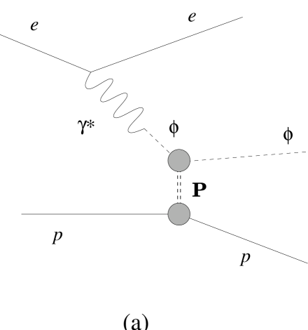
FIG. 2.: (a) Diffractive $\phi$ meson production within the vector-meson-dominance model by means of Pomeron exchange; (b) $s\bar{s}$-knockout and (c) $uud$-knockout contributions to $\phi$ meson electroproduction.

FIG. 3.: $\phi$ meson production with some intermediate hadronic exited states.

                 

FIG. 4.: The $Q^{2}$-dependence of the cross section $\sigma(Q^{2},W)$ at $W$=2.1 GeV and $E_{e}=11.5$ GeV in NRQM with (a) $B^{2}=10$ % and (b) $B^{2}=20$%. The diffractive cross section is given by the solid line, the $s\bar{s}$- and $uud$-knockout cross sections are by the dotted and dashed lines, respectively, and the interference term is by the dash-dotted line.

                 

FIG. 5.: The $t$-dependence of the cross section $\sigma(Q^{2},W,t)$ at $W$=2.1 GeV, $E_{e}=11.5$ GeV, and $Q^{2}=0.02$ GeV² with (a) $B^{2}=10$ % and (b) $B^{2}=20$%. Notations are the same as in Fig. 4.

                 

FIG. 6.: The $t$-dependence of the cross section $\sigma(Q^{2},W,t)$ at $W$=2.1 GeV, $E_{e}=11.5$ GeV, and $Q^{2}=0.5$ GeV² with (a) $B^{2}=10$ % and (b) $B^{2}=20$%. Notations are the same as in Fig. 4.

FIG. 7.: The $t$ dependence of $q_{1}^{2}$ and $q_{2}^{2}$ in the RHOM overlap integrals at $Q^{2}=0.5$ GeV². The solid line is the value of $\mathchoice{{\hbox{\boldmath$\displaystyle q$}}}{{\hbox{\boldmath$\textstyle q$}}}{{\hbox{\boldmath$\scriptstyle q$}}}{{\hbox{\boldmath$\scriptscriptstyle q$}}}^{2}$, and the dotted and dot-dashed lines are $q_{1}^{2}$ and $q_{2}^{2}$, respectively.

                 

FIG. 8.: The $Q^{2}$-dependence of the cross section $\sigma(Q^{2},W)$ at $W$=2.1 GeV and $E_{e}=11.5$ GeV in RHOM with (a) $B^{2}=3$ % and (b) $B^{2}=5$%. Notations are the same as in Fig. 4.

                 

FIG. 9.: The $t$-dependence of the cross section $\sigma(Q^{2},W,t)$ at $W$=2.1 GeV, $E_{e}=11.5$ GeV, and $Q^{2}=0.02$ GeV² with (a) $B^{2}=3$ % and (b) $B^{2}=5$%. Notations are the same as in Fig. 4.

                 

FIG. 10.: The $t$-dependence of the cross section $\sigma(Q^{2},W,t)$ at $W$=2.1 GeV, $E_{e}=11.5$ GeV, and $Q^{2}=0.5$ GeV² with (a) $B^{2}=3$ % and (b) $B^{2}=5$%. Notations are the same as in Fig. 4.

                 

FIG. 11.: The $t$-dependence of the cross section $\sigma(Q^{2},W,t)$ at $W$=2.1 GeV, $E_{e}=11.5$ GeV, and $Q^{2}=1.0$ GeV² with (a) $B^{2}=3$ % and (b) $B^{2}=5$%. Notations are the same as in Fig. 4.

FIG. 12.: Prediction of the cloudy bag model on the probabilities of meson clouds in proton as a function of bag radius $R_{B}$ (in fm). The solid line represents the probability of the bare proton, the dotted line the $\pi$ cloud, the dashed (dot-dashed) line the $K$ ($\eta$) cloud. The dashed and dot-dashed lines are exaggerated by 5 and 10 times, respectively.

REFERENCES

• [1] See, for example, F. E. Close, An Introduction to Quarks and Partons (Academic Press, London, 1979).
• [2] T. P. Cheng and R. F. Dashen, Phys. Rev. Lett. 26 (1971) 594; T. P. Cheng, Phys. Rev. D 13 (1976) 2161; J. F. Donoghue and C. R. Nappi, Phys. Lett. B 168 (1986) 105; J. Gasser, H. Leutwyler and M. E. Sainio, Phys. Lett. B 253 (1991) 252.
• [3] EM Collaboration, J. Ashman et al., Phys. Lett. B 206 (1988) 364; Nucl. Phys. B 328 (1989) 1.
• [4] For more recent measurements, see e.g., SM Collaboration, D. Adams et al., Phys. Lett. B 329 (1994) 399.
• [5] L. A. Ahrens et al., Phys. Rev. D 35 (1987) 785; G. T. Garvey, W. C. Louis and D. H. White, Phys. Rev. C 48 (1993) 761.
• [6] See, for instance, E. J. Beise and R. D. McKeown, Comments Nucl. Part. Phys. 20 (1991) 105.
• [7] M. Anselmino and M. D. Scadron, Phys. Lett. B 229 (1989) 117; H. J. Lipkin, Phys. Lett. B 256 (1991) 284; R. L. Jaffe and H. J. Lipkin, Phys. Lett. B 266 (1991) 458.
• [8] D. B. Kaplan and A. Manohar, Nucl. Phys. B 310 (1988) 527; D. H. Beck, Phys. Rev. D 39 (1989) 3248; R. D. McKeown, Phys. Lett. B 219 (1989) 140; D. B. Kaplan, Phys. Lett. B 275 (1992) 137.
• [9] E. M. Henley, G. Krein, S. J. Pollock and A. G. Williams, Phys. Lett. B 269 (1991) 31.
• [10] E. M. Henley, G. Krein and A. G. Williams, Phys. Lett. B 281 (1992) 178.
• [11] J. Ellis, E. Gabathuler and M. Karliner, Phys. Lett. B 217 (1989) 173.
• [12] J. Ellis and M. Kaliner, Invited lectures at the International School of Nucleon Spin Structure, Erice, 1995, CERN Report No. CERN-TH/95-334, (1995), hep-ph/9601280, and references therein.
• [13] J. Ellis, M. Karliner, D. E. Kharzeev and M. G. Sapozhnikov, Phys. Lett. B 353 (1995) 319; For a recent experiment, see, OBELIX Collaboration, A. Bertin et al., Phys. Lett. B 388 (1996) 450.
• [14] For old experiments on $\phi$ electroproduction, see, for instance, R. Dixon et al., Phys. Rev. Lett. 39 (1977) 516; R. Dixon et al., Phys. Rev. D 19 (1979) 3185;
• [15] D. G. Cassel et al., Phys. Rev. D 24 (1981) 2787 and references therein.
• [16] ZEUS Collaboration, M. Derrick et al., Phys. Lett. B 380 (1996) 220.
• [17] A. I. Titov, Y. Oh and S. N. Yang, Chin. J. Phys. (Taipei) 32 (1994) 1351.
• [18] H. Yukawa, Phys. Rev. 91 (1953) 416; M. A. Markov, Hyperons and K Mesons (Fizmatgiz, Moscow, 1958).
• [19] K. Fujimura, T. Kobayashi and M. Namiki, Prog. Theor. Phys. 44 (1970) 193; Prog. Theor. Phys. 43 (1970) 73.
• [20] R. P. Feynman, M. Kisslinger and F. Ravndal, Phys. Rev. D 3 (1971) 2706.
• [21] R. G. Lipes, Phys. Rev. D 5 (1972) 2849.
• [22] Y. S. Kim and M. E. Noz, Phys. Rev. D 12 (1975) 129.
• [23] Y. Kizukuri, M. Namiki and K. Okano, Prog. Theor. Phys. 61 (1979) 559.
• [24] V. V. Burov, S. M. Dorkin, V. K. Lukyanov and A. I. Titov, Z. Phys. A 306 (1982) 149.
• [25] Y. Fujiwara and K. T. Hecht, Nucl. Phys. A 444 (1985) 541; R. Müller and H. M. Hofmann, Phys. Rev. Lett. 65 (1990) 3245.
• [26] H. Fraas and D. Schildknecht, Nucl. Phys. B 14 (1969) 543; P. Joos et al., Nucl. Phys. B 113 (1976) 577.
• [27] R. H. Dalitz and D. R. Yennie, Phys. Rev. 105 (1957) 1598; C. W. Akerlof et al., Phys. Rev. 163 (1967) 1482; T. Abdullah and F. E. Close, Phys. Rev. D 5 (1972) 2332; M. Warns, H. Schröder, W. Pfeil and H. Rollnik, Z. Phys. C 45 (1990) 613.
• [28] R. P. Feynman, Photon-Hadron Interactions (W.A. Benjamin, Reading, 1972).
• [29] S. J. Brodsky and J. R. Primack, Ann. Phys. (N.Y.) 52 (1969) 315; F. E. Close and Z. Li, Phys. Rev. D 42 (1990) 2194.
• [30] A. I. Titov and S. N. Yang, in Proceedings of the 13th International Conference on Particle and Nuclei, Perugia, Italy, 1993, edited by A. Pascolini (World Scientific, Singapore, 1994), p. 625.
• [31] Jaffe and Lipkin in Ref. [7].
• [32] J. Keppler and H. M. Hofmann, Phys. Rev. D 51 (1995) 3936.
• [33] S. Théberge, A. W. Thomas and G. A. Miller, Phys. Rev. D 22 (1980) 2838; A. W. Thomas, S. Théberge and G. A. Miller, Phys. Rev. D 24 (1981) 216.
• [34] P. Żenczykowski, Phys. Rev. D 29 (1984) 577; E. A. Veit, B. K. Jennings, A. W. Thomas and R. C. Barrett, Phys. Rev. D 31 (1985) 1033.
• [35] V. A. Matveev and P. Sorba, Lett. Nuovo Cimento 20 (1977) 435; S. M. Dorkin, V. K. Lukyanov and A. I. Titov, Z. Phys. A 316 (1984) 331.
• [36] F. Myhrer, in Quarks and Nuclei, International Review of Nuclear Physics, Vol. 1, edited by W. Weise (World Scientific, Singapore, 1984).
• [37] D. Klabučar and G. E. Brown, Nucl. Phys. A 454 (1986) 589; A. Hosaka, H. Toki and W. Weise, Nucl. Phys. A 506 (1990) 501; A. Hosaka, Nucl. Phys. A 546 (1992) 493.
• [38] A. I. Titov, S. N. Yang and Y. Oh, in preparation.
Refer to caption