The Dirac-Brueckner Approach

1 Introduction

One of the most fundamental challenges pervading theoretical nuclear physics since half a century is to understand the properties of nuclei in terms of the underlying interactions between the constituents.

Historically, the first attempt was made by Heisenberg’s student H. Euler who calculated the properties of nuclear matter in second order perturbation theory [1] assuming nucleons interacting via a two-body potential of Gaussian shape. When the singular nature of the nuclear potential at short distances (’hard core’) was realized, it became apparent that conventional perturbation theory is inadequate. Special many-body methods had to be worked out. Brueckner and coworkers [2] initiated a method which was further developed by Bethe [3] and Goldstone [4]. Alternatively, Jastrow [5] suggested to take a variational approach to the nuclear many-body problem.

In the 1960’s, substantial advances in the physical understanding of Brueckner theory were made due to the work by Bethe and coworkers (see e. g. the review by Day [6]). Systematic calculations of the properties of nuclear matter applying Brueckner theory started in the late 1960’s and continued through the 1970’s [7-9] (see Ref. [10] for a more recent summary).

The results obtained using a variety of nucleon-nucleon (NN) potentials show a systematic behaviour: The predictions for nuclear matter saturation are located along a band which does not meet the empirical area, see Fig. 1 and Table 1. (Various semi-empirical sources suggest nuclear matter saturation to occur at an energy per particle ${\cal E}/A=-16\pm 1$ MeV and a density which is equivalent to a Fermi momentum of $k_{F}=1.35\pm 0.05$ fm^-1 [8, 9].) This phenomenon is denoted by the ”Coester band” [22]. The essential parameter of the Coester band is the strength of the nuclear tensor force as measured by the predicted D-state probability of the deuteron or as expressed in terms of the wound integral in nuclear matter (see Table 1) [10].

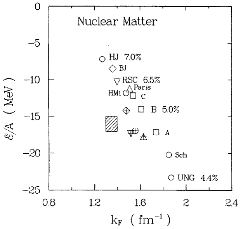
Figure 1: Nuclear matter saturation as predicted by a variety of NN potentials (cf. Table 1). Open symbols are saturation points obtained in the two-hole line approximation, symbols with a cross denote corresponding predictions with three- and four-hole lines included. %-numbers refer to the D-state probability of the deuteron as predicted by the corresponding potential. The shaded area denotes the empirical value.

Table 1: Nuclear matter saturation properties as predicted by various NN potentials.

Potential	Ref.a	$P_{D}$ (%)	$\kappa$ (%)	${\cal E}/A$ (MeV)	$k_{F}$ (fm-1)	Ref.b
HJ	11	7.0	21	–7.2	1.27	12
BJ	13	6.6	—	–8.5 [–14.2]	1.36 [1.48]	12
RSC	14	6.5	14	–10.3c [–17.3]	1.40c [1.52]	15 [12]
V14	16	6.1	12 [19]	–10.8 [–17.8]	1.47 [1.62]	17
Paris	18	5.8	11	–11.2 [–17.7]	1.51 [1.63]	18 [17]
HM1	19	5.8	11	–11.8 [–16.9]	1.48 [1.56]	19 [17]
Sch	20	4.9	8	–20.2	1.85	19
UNG	21	4.4	5	–23.3	1.87	19
Bonn C	10	5.6	8.1	–12.1	1.54	10
Bonn B	10	5.0	6.6	–14.0	1.61	10
Bonn A	10	4.4	5.4	–17.1	1.74	10
Given are the saturation energy per nucleon, ${\cal E}/A$, and Fermi momentum,
$k_{F}$, as obtained in the two-hole line approximation using the standard
choice for the single particle potential. Results including three- and four-
hole line contributions are given in square brakets. The wound integral
$\kappa$ is given at $k_{F}=1.35$ fm-1. $P_{D}$ is the predicted %-D state of the deuteron.
a References to the potentials.
b References for the nuclear matter calculations.
c Using OBEP for $J\geq 3$.

The Brueckner-Goldstone expansion is believed to be convergent in terms of the number of hole lines. Calculations by Day [12, 23, 17] have confirmed this for the case of some realistic potentials. However, three- and four-hole line diagrams contribute about 5-7 MeV to the binding energy per nucleon at saturation (cf. Table 1) and, thus, are not negligible. In Fig. 1 open symbols represent results obtained in the two-hole line approximation, symbols with a cross denote results including the contributions from three and four hole-lines. It is seen that taking into account up to four hole lines leads, indeed, to an improved Coester band as compared to the two-hole line approximation; however, the improvement is insufficient to explain the empirical saturation point [24]. Results based on the variational approach are in fair agreement with Brueckner theory predictions [17] and, thus, also fail to quantitatively explain nuclear saturation.

Since the mid 1970’s, there have been comprehensive efforts to check Brueckner theory [25]; we mention here, in particular, the work using hypernetted chain theory [25, 26]. Based on this work, there are indications that the two hole-line approximation of Brueckner-Bethe theory may not necessarily be correct. Some published variational calculations are in fair agreement with Brueckner-Bethe results if three hole-lines plus a four hole-line estimate are included [17].

Approaches discussed so far are based on the simplest model for the atomic nucleus: Nucleons obeying the non-relativistic Schrödinger equation interact through a two-body potential that fits low-energy NN scattering data and the properties of the deuteron. The failure of this model to explain nuclear saturation indicates that we may have to extend the model. One possibility is to include degrees of freedom other than the nucleon. The meson theory of the nuclear force suggests to consider, particularly, meson and isobar degrees of freedom. Characteristically, these degrees of freedom lead to medium effects on the nuclear force when inserted into the many-body problem as well as many-nucleon force contributions (see Ref. [10] for a comprehensive review on this subject). In general, the medium effects are repulsive whereas the many-nucleon force contributions are attractive. Thus, there are large cancellations and the net result is very small. The density dependence of these effects/contributions is such that the saturation properties of nuclear matter are not improved [10].

We note that the discussion of many-body force effects in the previous paragraph applies to approaches in which two- and many-body forces are treated on an equal footing; i. e. both categories of forces are based on the same meson-baryon interactions and are treated consistently. The situation is different if the three-body force is introduced on an ad hoc basis with the purpose to fit the empirical nuclear matter saturation [27]. Such a three-body potential may be large, particularly, if the two-body force used substantially underbinds nuclear matter. By construction such a three-body force improves the equation of state of nuclear matter as well as the description of light nuclei.

In the 1970’s, a relativistic approach to nuclear structure was developed by Miller and Green [28]. They studied a Dirac-Hartree model for the groundstate of nuclei which was able to reproduce the binding energies, the root-mean-square radii, and the single-particle levels, particularly, the spin-orbit splittings. Their potential consisted of a strong (attractive) scalar and (repulsive) vector component. The Dirac-Hartree(-Fock) model was further developed by Brockmann [29] and by Horowitz and Serot [30, 31]. At about that same time, Clark and coworkers applied a Dirac equation containing a scalar and vector field to proton-nucleus scattering [32]. The most significant result of this Dirac phenomenology is the quantitative fit of spin observables which were only poorly described by the Schrödinger equation [33]. This success and Walecka’s theory on highly condensed matter [34] made relativistic approaches very popular.

Inspired by these achievements, a relativistic extension of Brueckner theory has been suggested by Shakin and collaborators [35, 36], frequently called the Dirac-Brueckner approach. The advantage of a Brueckner theory is that the free NN interaction is used; thus, there are no parameters in the force which are adjusted in the many-body problem. The essential point of the Dirac-Brueckner approach is to use the Dirac equation for the single particle motion in nuclear matter. In the work done by the Brooklyn group the relativistic effect is calculated in first order perturbation theory. This approximation is avoided and a full self-consistency of the relativistic single-particle energies and wave functions is performed in the subsequent work by Brockmann and Machleidt [37, 38, 39], and by ter Haar and Malfliet [40]. Formal aspects involved in the derivation of the relativistic G-matrix, have been discussed in detail by Horowitz and Serot [41, 42].

The common feature of all Dirac-Brueckner results is that a (repulsive) relativistic many-body effect is obtained which is strongly density-dependent such that the empirical nuclear matter saturation can be explained. In most calculations a one-boson-exchange (OBE) potential is used for the nuclear force. In Ref. [43] a more realistic approach to the NN interaction is taken applying an explicit model for the 2$\pi$-exchange that involves $\Delta$-isobars, thus, avoiding the fictitious $\sigma$ boson typically used in OBE models to provide intermediate range attraction. It is found in Ref. [43] that the relativistic effect for the more realistic model is almost exactly the same as that obtained for OBE potentials. This finding seems to justify the use of the OBE model.

It is the purpose of this chapter to present a thorough introduction into the Dirac Brueckner approach including the mathematical details of the formalism involved. Furthermore, we will present results for nuclear matter, NN scattering in the nuclear medium, and finite nuclei.

2 Relativistic Two-Nucleon Scattering

2.1 Covariant Equations

Two-nucleon scattering is described covariantly by the Bethe-Salpeter (BS) equation [44]. In operator notation it may be written as

$${\cal M=V+VGM}$$ (1)

with ${\cal M}$ the invariant amplitude for the two-nucleon scattering process, ${\cal V}$ the sum of all connected two-particle irreducible diagrams and ${\cal G}$ the relativistic two-nucleon propagator. As this four-dimensional integral equation is very difficult to solve [45], so-called three-dimensional reductions have been proposed, which are more amenable to numerical solution. Furthermore, it has been shown by Gross [46] that the full BS equation in ladder approximation does not generate the desired one-body equation in the one-body limit (i. e., when one of the particles becomes very massive) in contrast to a large family of three-dimensional quasi-potential equations. These approximations to the BS equation are also covariant and satisfy relativistic elastic unitarity. However, the three-dimensional reduction is not unique, and in principal infinitely many choices exist [47]. Typically they are derived by replacing Eq. (1) by two coupled equations:

$${\cal M=W+W}g{\cal M}$$ (2)

and

$${\cal W=V+V(G}-g){\cal W}$$ (3)

where $g$ is a covariant three-dimensional propagator with the same elastic unitarity cut as ${\cal G}$ in the physical region. In general, the second term on the r.h.s. of Eq. (3) is dropped to arrive at a real simplification of the problem.

Explicitly, we can write the BS equation for an arbitrary frame (notation and conventions of Ref. [48])

$${\cal M}(q^{\prime},q|P)={\cal V}(q^{\prime},q|P)+\int d^{4}k{\cal V}(q^{\prime},k|P){\cal G}(k|P){\cal M}(k,q|P)$$ (4)

with

$${\cal G}(k|P) = \frac{i}{(2\pi)^{4}}\frac{1}{(\frac{1}{2}\not\!P+\not\!k-M+i\epsilon)^{(1)}}\frac{1}{(\frac{1}{2}\not\!P-\not\!k-M+i\epsilon)^{(2)}}$$ (5)

$$= \frac{i}{(2\pi)^{4}}\left[\frac{\frac{1}{2}\not\!P+\not\!k+M}{(\frac{1}{2}P+k)^{2}-M^{2}+i\epsilon}\right]^{(1)}\left[\frac{\frac{1}{2}\not\!P-\not\!k+M}{(\frac{1}{2}P-k)^{2}-M^{2}+i\epsilon}\right]^{(2)}$$ (6)

where $q$, $k$, and $q^{\prime}$ are the initial, intermediate, and final relative four-momenta, respectively (with e. g. $k=(k_{0},{\bf k})$), and $P=(P_{0},{\bf P})$ is the total four-momentum; $\not\!k=\gamma^{\mu}k_{\mu}$. The superscripts refer to particle (1) and (2). In general, we suppress spin (or helicity) and isospin indices.

${\cal G}$ and $g$ have the same discontinuity across the right hand cut, if

$${\rm Im}\>{\cal G}(k|P) = -\frac{2\pi^{2}}{(2\pi)^{4}}\left[\>\frac{1}{2}\not\!P+\not\!k+M\>\right]^{(1)}\;\left[\>\frac{1}{2}\not\!P-\not\!k+M\>\right]^{(2)}$$ (7)

$$\times\delta^{(+)}\left[\>\left(\,\frac{1}{2}\,P+k\right)^{2}-M^{2}\right]\;\delta^{(+)}\left[\>\left(\,\frac{1}{2}\,P-k\right)^{2}-M^{2}\right]$$

$$= {\rm Im}\>g(k|P)$$

with $\delta^{(+)}$ indicating that only the positive energy root of the argument of the $\delta$-function is to be included. From this follows easily

$${\rm Im}\>g(k|P) = -\frac{1}{8\pi^{2}}\left[\>\frac{1}{2}\not\!P+\not\!k+M\>\right]^{(1)}\;\left[\>\frac{1}{2}\not\!P-\not\!k+M\>\right]^{(2)}$$ (8)

$$\times\frac{\delta\left(\frac{1}{2}P_{0}+k_{0}-E_{\frac{1}{2}{\bf P}+{\bf k}}\right)\delta\left(\frac{1}{2}P_{0}-k_{0}-E_{\frac{1}{2}{\bf P}-{\bf k}}\right)}{4\,E_{\frac{1}{2}{\bf P}+{\bf k}}\,E_{\frac{1}{2}{\bf P}-{\bf k}}}$$

with $E_{\frac{1}{2}{\bf P}\pm{\bf k}}\equiv\sqrt{M^{2}+(\frac{1}{2}{\bf P}\pm{\bf k})^{2}}$. Using the equality

$$\delta\left(\frac{1}{2}P_{0}+k_{0}-E_{\frac{1}{2}{\bf P}+{\bf k}}\right)\delta\left(\frac{1}{2}P_{0}-k_{0}-E_{\frac{1}{2}{\bf P}-{\bf k}}\right)=$$ (9)

$$\delta\left(P_{0}-E_{\frac{1}{2}{\bf P}+{\bf k}}-E_{\frac{1}{2}{\bf P}-{\bf k}}\right)\delta\left(k_{0}-\frac{1}{2}E_{\frac{1}{2}{\bf P}+{\bf k}}+\frac{1}{2}E_{\frac{1}{2}{\bf P}-{\bf k}}\right)$$

the imaginary part of the propagator $g(k|P)$ can now be written

$${\rm Im}\>g(k|P) = -\frac{1}{8\pi^{2}}\frac{M^{2}}{E_{\frac{1}{2}{\bf P}+{\bf k}}\>E_{\frac{1}{2}{\bf P}-{\bf k}}}\Lambda_{+}^{(1)}\left(\frac{1}{2}{\bf P}+{\bf k}\right)\>\Lambda_{+}^{(2)}\left(\frac{1}{2}{\bf P}-{\bf k}\right)$$ (10)

$$\times\delta\left(P_{0}-E_{\frac{1}{2}{\bf P}+{\bf k}}-E_{\frac{1}{2}{\bf P}-{\bf k}}\right)$$

$$\times\delta\left(k_{0}-\frac{1}{2}E_{\frac{1}{2}{\bf P}+{\bf k}}+\frac{1}{2}E_{\frac{1}{2}{\bf P}-{\bf k}}\right)$$

where

$$\Lambda_{+}^{(i)}({\bf p}) = \left(\frac{\gamma^{0}E_{\bf p}-\mbox{\boldmath$\gamma$}\cdot{\bf p}+M}{2M}\right)^{(i)}$$ (11)

$$= \sum_{\lambda_{i}}\>u({\bf p},\lambda_{i})\overline{u}({\bf p},\lambda_{i})$$ (12)

represents the positive-energy projection operator for nucleon $i$ ($i=1,2$) with $u({\bf p})$ a positive-energy Dirac spinor of momentum $\bf p$; $\lambda_{i}$ denotes either the helicity or the spin projection of the respective nucleon, and $E_{\bf p}=\sqrt{M^{2}+{\bf p}^{2}}$. The projection operators imply that contributions involving virtual anti-nucleon intermediate states (‘pair terms’) are suppressed. It has been shown in Refs. [49, 50] that these contributions are small when the pseudovector coupling is used for the pion.

Note that ${\rm Im}\>g(k|P)$ is covariant, since ${\rm Im}\>g(k|P)={\rm Im}\>{\cal G}(k|P)$.

Using $\delta(P_{0}-E)=2E\delta(s-E^{2}+{\bf P}^{2})$, where $E=E_{\frac{1}{2}{\bf P}+{\bf k}}+E_{\frac{1}{2}{\bf P}-{\bf k}}$ and $s=P^{2}=P_{0}^{2}-{\bf P}^{2}$,  Eq. (10) can be re-written as

$${\rm Im}\>g(k|s) = -\frac{M^{2}}{8\pi^{2}}\,\frac{2\left(E_{\frac{1}{2}{\bf P}+{\bf k}}+E_{\frac{1}{2}{\bf P}-{\bf k}}\right)}{E_{\frac{1}{2}{\bf P}+{\bf k}}E_{\frac{1}{2}{\bf P}-{\bf k}}}\Lambda_{+}^{(1)}\left(\frac{1}{2}{\bf P}+{\bf k}\right)\Lambda_{+}^{(2)}\left(\frac{1}{2}{\bf P}-{\bf k}\right)$$ (13)

$$\times\delta\left[s-\left(E_{\frac{1}{2}{\bf P}+{\bf k}}+E_{\frac{1}{2}{\bf P}-{\bf k}}\right)^{2}+{\bf P}^{2}\right]$$

$$\times\delta\left(k_{0}-\frac{1}{2}E_{\frac{1}{2}{\bf P}+{\bf k}}+\frac{1}{2}E_{\frac{1}{2}{\bf P}-{\bf k}}\right)$$

Knowing its imaginary part, we construct $g(k|s)$ by a dispersion integral

$$g(k|s)=\frac{1}{\pi}\int^{\infty}_{4M^{2}}\frac{ds^{\prime}}{s^{\prime}-s-i\epsilon}{\rm Im}g(k|s^{\prime})$$ (14)

Inserting Eq. (13) in Eq. (14) and integrating, we obtain

$$g(k|P) = -\frac{M^{2}}{(2\pi)^{3}}\frac{2\left(E_{\frac{1}{2}{\bf P}+{\bf k}}+E_{\frac{1}{2}{\bf P}-{\bf k}}\right)}{E_{\frac{1}{2}{\bf P}+{\bf k}}E_{\frac{1}{2}{\bf P}-{\bf k}}}$$ (16)

$$\times\frac{\Lambda_{+}^{(1)}\left(\frac{1}{2}{\bf P}+{\bf k}\right)\Lambda_{+}^{(2)}\left(\frac{1}{2}{\bf P}-{\bf k}\right)}{\left(E_{\frac{1}{2}{\bf P}+{\bf k}}+E_{\frac{1}{2}{\bf P}-{\bf k}}\right)^{2}-{\bf P}^{2}-s-i\epsilon}$$

$$\times\delta(\begin{array}[]{c}k_{0}-\frac{1}{2}E_{\frac{1}{2}{\bf P}+{\bf k}}+\frac{1}{2}E_{\frac{1}{2}{\bf P}-{\bf k}}\end{array})$$

This three-dimensional propagator is known as the Blankenbecler-Sugar (BbS) choice [51, 52]. By construction, the propagator $g$ has the same discontinuity across the right-hand cut as ${\cal G}$; therefore, it preserves the unitarity relation satisfied by ${\cal M}$.

Using the angle averages $(\>\frac{1}{2}{\bf P}\pm{\bf k}\>)^{2}\approx\frac{1}{4}{\bf P}^{2}+{\bf k}^{2}$ and $(\>\frac{1}{2}{\bf P}\pm{\bf q}\>)^{2}\approx\frac{1}{4}{\bf P}^{2}+{\bf q}^{2}$, which should be a very good approximation, Eq. (15) assumes the much simpler form

$$g(k|P)=\frac{1}{(2\pi)^{3}}\frac{M^{2}}{E_{\frac{1}{2}{\bf P}+{\bf k}}}\frac{\Lambda_{+}^{(1)}\left(\frac{1}{2}{\bf P}+{\bf k}\right)\Lambda_{+}^{(2)}\left(\frac{1}{2}{\bf P}-{\bf k}\right)}{E_{\frac{1}{2}{\bf P}+{\bf q}}^{2}-E_{\frac{1}{2}{\bf P}+{\bf k}}^{2}+i\epsilon}\delta(k_{0})$$ (17)

where we used $s=4E^{2}_{\frac{1}{2}{\bf P}+{\bf q}}-{\bf P}^{2}$.

Assuming ${\cal W}={\cal V}$, the reduced Bethe-Salpeter equation, Eq. (2), is obtained in explicit form by replacing in Eq. (4) ${\cal G}$ by $g$ of Eq. (16), yielding

$${\cal M}({\bf q^{\prime}},{\bf q}|{\bf P}) = {\cal V}({\bf q^{\prime}},{\bf q}|{\bf P})+\int\frac{d^{3}k}{(2\pi)^{3}}{\cal V}({\bf q^{\prime}},{\bf k}|{\bf P})\frac{M^{2}}{E_{\frac{1}{2}{\bf P}+{\bf k}}}$$ (18)

$$\times\frac{\Lambda_{+}^{(1)}\left(\frac{1}{2}{\bf P}+{\bf k}\right)\Lambda_{+}^{(2)}\left(\frac{1}{2}{\bf P}-{\bf k}\right)}{E_{\frac{1}{2}{\bf P}+{\bf q}}^{2}-E_{\frac{1}{2}{\bf P}+{\bf k}}^{2}+i\epsilon}{\cal M}({\bf k},{\bf q}|{\bf P})$$

in which both nucleons in intermediate states are equally far off their mass shell.

Taking matrix elements between positive-energy spinors yields an equation for the scattering amplitude in an arbitrary frame

$${\cal T}({\bf q^{\prime}},{\bf q}|{\bf P}) = V({\bf q^{\prime}},{\bf q})+\int\frac{d^{3}k}{(2\pi)^{3}}V({\bf q^{\prime}},{\bf k})\frac{M^{2}}{E_{\frac{1}{2}{\bf P}+{\bf k}}}$$ (19)

$$\times\frac{1}{E_{\frac{1}{2}{\bf P}+{\bf q}}^{2}-E_{\frac{1}{2}{\bf P}+{\bf k}}^{2}+i\epsilon}{\cal T}({\bf k},{\bf q}|{\bf P})$$

where we used

$$\begin{array}[]{l}\bar{u}_{1}(\frac{1}{2}{\bf P}+{\bf q^{\prime}})\bar{u}_{2}(\frac{1}{2}{\bf P}-{\bf q^{\prime}}){\cal V}({\bf q^{\prime}},{\bf q}|{\bf P})u_{1}(\frac{1}{2}{\bf P}+{\bf q})u_{2}(\frac{1}{2}{\bf P}-{\bf q})=\end{array}$$ (22)

$$\bar{u}_{1}({\bf q^{\prime}})\bar{u}_{2}(-{\bf q^{\prime}}){\cal V}({\bf q^{\prime}},{\bf q})u_{1}({\bf q})u_{2}(-{\bf q})$$

$$\equiv V({\bf q^{\prime}},{\bf q})$$

since this is a Lorentz scalar. An analogous statement applies to ${\cal T}$. Calculations of nuclear matter and of finite nuclei are performed in the rest frames of these systems. Thus, Eq. (18) with the necessary medium modifications would be appropriate for the evaluation of the nuclear matter reaction ($G$) matrix.

In the two-nucleon c.m. frame ( i. e. for ${\bf P}=0$), the BbS propagator, Eq. (16), reduces to

$$g({\bf k},s)=\frac{1}{(2\pi)^{3}}\frac{M^{2}}{E_{\bf k}}\frac{\Lambda_{+}^{(1)}({\bf k})\Lambda_{+}^{(2)}({\bf-k})}{\frac{1}{4}s-E^{2}_{\bf k}+i\epsilon}\delta{(k_{0})}$$ (23)

which implies the scattering equation

$${\cal T}({\bf q^{\prime}},{\bf q})=V({\bf q^{\prime}},{\bf q})+\int\frac{d^{3}k}{(2\pi)^{3}}V({\bf q^{\prime}},{\bf k})\frac{M^{2}}{E_{\bf k}}\frac{1}{{\bf q}^{2}-{\bf k}^{2}+i\epsilon}{\cal T}({\bf k},{\bf q})$$ (24)

Two-nucleon scattering is considered most conveniently in the two-nucleon c.m. frame; thus, for calculations of free space two-nucleon scattering in the BbS approximation, one would use Eq. (21).

Defining

$$\hat{T}({\bf q^{\prime}},{\bf q})=\sqrt{\frac{M}{E_{q^{\prime}}}}\>{\cal T}({\bf q^{\prime}},{\bf q})\>\sqrt{\frac{M}{E_{q}}}$$ (25)

and

$$\hat{V}({\bf q^{\prime}},{\bf q})=\sqrt{\frac{M}{E_{q^{\prime}}}}\>V({\bf q^{\prime}},{\bf q})\>\sqrt{\frac{M}{E_{q}}},$$ (26)

which has become known as “minimal relativity” [53], we can rewrite Eq. (21) as

$$\hat{T}({\bf q^{\prime}},{\bf q})=\hat{V}({\bf q^{\prime}},{\bf q})+\int d^{3}k\>\hat{V}({\bf q^{\prime}},{\bf k})\>\frac{M}{{\bf q}^{2}-{\bf k}^{2}+i\epsilon}\>\hat{T}({\bf k},{\bf q})$$ (27)

which has the form of the non-relativistic Lippmann-Schwinger equation. A potential defined within an equation which is formally identical to the (non-relativistic) Lippmann-Schwinger equation, can then be applied in conventional (non-relativistic) nuclear structure physics. This is the practical relevance of Eqs. (22-24). On the other hand, for relativistic nuclear structure physics, Eq. (21) is the starting point.

The BbS propagator is the most widely used approximation. Another choice, that has been frequently applied, is the version suggested by Thompson [54]. The manifestly covariant form of Thompson’s propagator is the same as Eq. (14), but with $\int^{\infty}_{4M^{2}}ds^{\prime}/(s^{\prime}-s-i\epsilon)$ replaced by $\int^{\infty}_{2M}d\sqrt{s^{\prime}}/(\sqrt{s^{\prime}}-\sqrt{s}-i\epsilon)$. After taking the angle average for $|\>\frac{1}{2}{\bf P}\pm{\bf k}\>|$ and $|\>\frac{1}{2}{\bf P}\pm{\bf q}\>|$, this propagator reads

$$g(k|P)=\frac{1}{(2\pi)^{3}}\frac{M^{2}}{E_{\bf k}E_{\frac{1}{2}{\bf P}+{\bf k}}}\frac{\Lambda_{+}^{(1)}\left(\frac{1}{2}{\bf P}+{\bf k}\right)\Lambda_{+}^{(2)}\left(\frac{1}{2}{\bf P}-{\bf k}\right)}{2E_{\bf q}-2E_{\bf k}+i\epsilon}\delta(k_{0})$$ (28)

The equation for the scattering amplitude in an arbitrary frame is

$${\cal T}({\bf q^{\prime}},{\bf q}|{\bf P}) = V({\bf q^{\prime}},{\bf q})+\int\frac{d^{3}k}{(2\pi)^{3}}V({\bf q^{\prime}},{\bf k})\frac{M^{2}}{E_{\bf k}\>E_{\frac{1}{2}{\bf P}+{\bf k}}}$$ (29)

$$\times\frac{1}{2E_{\bf q}-2E_{\bf k}+i\epsilon}{\cal T}({\bf k},{\bf q}|{\bf P})$$

For calculations in the rest frame of nuclear matter or finite nuclei, this equation together with the necessary medium modifications ($M\longmapsto\tilde{M}$, Pauli projector $Q$) is appropriate (see Eq. (95) below). In our actual calculations in nuclear matter, we replace $E_{\bf k}$ by $E_{\frac{1}{2}{\bf P}+{\bf k}}$ and $E_{\bf q}$ by $E_{\frac{1}{2}{\bf P}+{\bf q}}$ in the denominator of Eq. (26). This replacement makes possible an interpretation of the energy denominator in terms of differences between single particle energies which are typically defined in the rest frame of the many-body system. This allows for a consistent application of this equation in nuclear matter and finite nuclei [55]. The change of the numerical results by this replacement is negligibly small (less than 0.1 MeV for the energy per nucleon at nuclear matter denisty), since the factor $\frac{M^{2}}{E_{\bf k}\>E_{\frac{1}{2}{\bf P}+{\bf k}}}$ is slightly reduced, while the term $(2E_{\bf q}-2E_{\bf k}+i\epsilon)^{-1}$ is slightly enhanced.

In the two-nucleon c.m. frame (${\bf P}=0$), the Thompson equation is

$${\cal T}({\bf q^{\prime}},{\bf q})=V({\bf q^{\prime}},{\bf q})+\int\frac{d^{3}k}{(2\pi)^{3}}V({\bf q^{\prime}},{\bf k})\frac{M^{2}}{E_{\bf k}^{2}}\frac{1}{2E_{\bf q}-2E_{\bf k}+i\epsilon}{\cal T}({\bf k},{\bf q}),$$ (30)

This equation is usefull for free-space two-nucleon scattering. In the calculations of this chapter, always Thompson’s equations are used.

Again, we may introduce some special definitions. In the case of the Thompson equation, it is convenient to define

$$\check{T}({\bf q^{\prime}},{\bf q})={\frac{M}{E_{q^{\prime}}}}\>{\cal T}({\bf q^{\prime}},{\bf q})\>{\frac{M}{E_{q}}}$$ (31)

and

$$\check{V}({\bf q^{\prime}},{\bf q})={\frac{M}{E_{q^{\prime}}}}\>V({\bf q^{\prime}},{\bf q})\>{\frac{M}{E_{q}}}\>.$$ (32)

With this, we can rewrite Eq. (27) as

$$\check{T}({\bf q^{\prime}},{\bf q})=\check{V}({\bf q^{\prime}},{\bf q})+\int d^{3}k\>\check{V}({\bf q^{\prime}},{\bf k})\frac{1}{2E_{q}-2E_{k}+i\epsilon}\check{T}({\bf k},{\bf q})$$ (33)

which looks like a Lippmann-Schwinger equation with relativistic energies in the propagator.

Since both nucleons are equally off-shell in the BbS or Thompson equation, the exchanged bosons tranfer three-momentum only, i. e. the meson propagator is (for a scalar exchange)

$$\frac{i}{-({\bf q^{\prime}-q})^{2}-m_{\alpha}^{2}};$$ (34)

this is also referred to as a static (or non-retarded) propagator.

Many more choices for $g$ have been suggested in the literature. For most of the other choices, the three-dimensional two-nucleon propagator is either of the BbS or the Thompson form. However, there may be differences in the $\delta$ function in Eqs. (20) and (25). For example, Schierholz [20] and Erkelenz [56] propose $\delta(k_{0}+\frac{1}{2}\sqrt{s}-E_{k})$, restricting one particle to its mass shell. It implies the meson propagator

$$\frac{i}{(E_{{\bf q}^{\prime}}-E_{{\bf q}})^{2}-({\bf q^{\prime}-q})^{2}-m_{\alpha}^{2}}.$$ (35)

However, it has been shown [57] (see also Appendix E.1 of Ref. [58]) that the term $(E_{{\bf q}^{\prime}}-E_{{\bf q}})^{2}$ in this propagator has an effect which is opposite to the one obtained when treating meson retardation properly. Also, the medium effect on meson propagation in nuclear matter which, when calculated correctly, is repulsive [59], comes out attractive when using the form Eq. (32) [60]. Thus, in spite of its suggestive appearance and in spite of early believes, the meson propagator Eq. (32) has nothing to do with genuine meson retardation and, therefore, should be discarded. This remark applies to the scattering of two particles of equal mass. If one particle is much heavier than the other one, it may, however, be appropriate to put one particle (namely, the more massive one) on its mass shell.

A thorough discussion of the Bethe-Salpeter equation and/or a systematic study of a large family of possible relativistic three-dimensional reductions can be found in Refs. [61, 62, 63]. Tjon and coworkers have compared results obtained by solving the full four-dimensional Bethe-Salpeter equation applying a full set of OBE diagrams with those from the BbS and some other three-dimensional equations; for BbS they find only small differences as compared to full BS [49, 50]. This is also true for the Thompson choice, since it differs little from BbS.

Notice that the quantity $\cal T$ in Eqs. (21) and (27) is invariant, while $\hat{T}$ of Eq. (24) and $\check{T}$ of Eq. (30) are not. $\hat{T}$ is equivalent to the familiar non-relativistic $T$-matrix.

The relationship of the invariant $\cal T$ to the $S$-matrix is

$$\langle p_{1}^{\prime}p_{2}^{\prime}|S|p_{1}p_{2}\rangle=\langle p_{1}^{\prime}p_{2}^{\prime}|p_{1}p_{2}\rangle-2\pi i\delta^{(4)}(p_{1}^{\prime}+p_{2}^{\prime}-p_{1}-p_{2})\frac{M^{2}}{E_{q}^{2}}{\cal T}({\bf q^{\prime},q})$$

with $p_{i}$ the initial and $p_{i}^{\prime}$ ($i=1,2$) the final four momenta of the two interacting nucleons. The normalization is $\langle p^{\prime}|p\rangle=\delta^{(3)}({\bf p^{\prime}-p})$.

2.2 R-Matrix Equation and Helicity State Basis

On a computer, real analysis is much faster than complex analysis. It is therefore desirable to deal with real quantities whenever possible. The scattering amplitude below particle production threshold can be expressed in terms of the real $R$-matrix (better known as the ‘$K$-matrix’) which is defined by

$$T=R-i\pi R\delta(E-H_{0})T$$ (37)

The equation for the real $\hat{R}$-matrix corresponding to the complex $\hat{T}$-matrix of Eq. (24) is

$$\hat{R}({\bf q^{\prime}},{\bf q})=\hat{V}({\bf q^{\prime}},{\bf q})+{\cal P}\int d^{3}k\>\hat{V}({\bf q^{\prime}},{\bf k})\>\frac{M}{{\bf q}^{2}-{\bf k}^{2}}\>\hat{R}({\bf k},{\bf q})$$ (38)

where ${\cal P}$ denotes the principal value.

Now, we also need to consider the spin of the nucleons explicitly. The easiest way to treat the spin-projections of spin-$\frac{1}{2}$ particles in a covariant way is to use the helicity representation. In our further developments, we will therefore use a helicity state basis (cf. Appendix C of Ref. [58] which is based upon Refs. [64, 65].

The helicity $\lambda_{i}$ of particle $i$ (with $i=1$ or 2) is the eigenvalue of the helicity operator $\frac{1}{2}{\bf\sigma}_{i}\cdot{\bf p}_{i}/|{\bf p}_{i}|$ which is $\pm\frac{1}{2}$.

Using helicity states, the $\hat{R}$-matrix equation reads, after partial wave decomposition,

$$\langle\lambda_{1}^{\prime}\lambda_{2}^{\prime}|\hat{R}^{J}(q^{\prime},q)|\lambda_{1}\lambda_{2}\rangle = \langle\lambda_{1}^{\prime}\lambda_{2}^{\prime}|\hat{V}^{J}(q^{\prime},q)|\lambda_{1}\lambda_{2}\rangle$$ (39)

$$\mbox{}+\sum_{h_{1},h_{2}}{\cal P}\int^{\infty}_{0}dk\>k^{2}\frac{M}{q^{2}-k^{2}}\langle\lambda_{1}^{\prime}\lambda_{2}^{\prime}|\hat{V}^{J}(q^{\prime},k)|h_{1}h_{2}\rangle$$

$$\mbox{}\times\langle h_{1}h_{2}|\hat{R}^{J}(k,q)|\lambda_{1}\lambda_{2}\rangle$$

where $J$ denotes the total angular momentum of the two nucleons. Here and throughout the rest of this chapter, momenta denoted by non-bold letters are the magnitudes of three-momenta, e. g. $q\equiv|{\bf q}|$, $k\equiv|{\bf k}|$, etc.; $h_{1}$ and $h_{2}$ are the helicities in intermediate states for nucleon 1 and 2, respectively. Equation (39) is a system of coupled integral equations which needs to be solved to obtain the desired matrix elements of $\hat{R}^{J}$.

Ignoring anti-particles, there are $4\times 4=16$ helicity amplitudes for $\hat{R}^{J}$. However, time-reversal invariance, parity conservation, and the fact that we are dealing with two identical fermions imply that only six amplitudes are independent. For these six amplitudes, we choose the following set:

$$\hat{R}^{J}_{1}(q^{\prime},q) \equiv \langle++|\hat{R}^{J}(q^{\prime},q)|++\rangle$$

$$\hat{R}^{J}_{2}(q^{\prime},q) \equiv \langle++|\hat{R}^{J}(q^{\prime},q)|--\rangle$$

$$\hat{R}^{J}_{3}(q^{\prime},q) \equiv \langle+-|\hat{R}^{J}(q^{\prime},q)|+-\rangle$$

$$\hat{R}^{J}_{4}(q^{\prime},q) \equiv \langle+-|\hat{R}^{J}(q^{\prime},q)|-+\rangle$$ (40)

$$\hat{R}^{J}_{5}(q^{\prime},q) \equiv \langle++|\hat{R}^{J}(q^{\prime},q)|+-\rangle$$

$$\hat{R}^{J}_{6}(q^{\prime},q) \equiv \langle+-|\hat{R}^{J}(q^{\prime},q)|++\rangle$$

where $\pm$ stands for $\pm\frac{1}{2}$. Notice that

$$\hat{R}^{J}_{5}(q^{\prime},q)=\hat{R}^{J}_{6}(q,q^{\prime}).$$ (41)

We have now six coupled equations. To partially decouple this system, it is usefull to introduce the following linear combinations of helicity amplitudes:

$${}^{0}\hat{R}^{J} \equiv \hat{R}^{J}_{1}-\hat{R}^{J}_{2}$$

$${}^{1}\hat{R}^{J} \equiv \hat{R}^{J}_{3}-\hat{R}^{J}_{4}$$

$${}^{12}\hat{R}^{J} \equiv \hat{R}^{J}_{1}+\hat{R}^{J}_{2}$$ (42)

$${}^{34}\hat{R}^{J} \equiv \hat{R}^{J}_{3}+\hat{R}^{J}_{4}$$

$${}^{55}\hat{R}^{J} \equiv 2\hat{R}^{J}_{5}$$

$${}^{66}\hat{R}^{J} \equiv 2\hat{R}^{J}_{6}$$

We also introduce corresponding definitions for $\hat{V}^{J}$. (Of course, analogous definitions exist for $R,\check{R},V,\mbox{ and }\check{V}$.) Using these definitions, Eq. (39) decouples into the following three sub-systems of integral equations:
Spin singlet

$${}^{0}\hat{R}^{J}(q^{\prime},q)=\>^{0}\hat{V}^{J}(q^{\prime},q)+{\cal P}\int^{\infty}_{0}dk\>k^{2}\frac{M}{q^{2}-k^{2}}\>^{0}\hat{V}^{J}(q^{\prime},k)\>^{0}\hat{R}^{J}(k,q)$$ (43)

Uncoupled spin triplet

$${}^{1}\hat{R}^{J}(q^{\prime},q)=\>^{1}\hat{V}^{J}(q^{\prime},q)+{\cal P}\int^{\infty}_{0}dk\>k^{2}\frac{M}{q^{2}-k^{2}}\>^{1}\hat{V}^{J}(q^{\prime},k)\>^{1}\hat{R}^{J}(k,q)$$ (44)

Coupled triplet states

$${}^{12}\hat{R}^{J}(q^{\prime},q) = {}^{12}\hat{V}^{J}(q^{\prime},q)+{\cal P}\int^{\infty}_{0}dk\>k^{2}\frac{M}{q^{2}-k^{2}}[\>^{12}\hat{V}^{J}(q^{\prime},k)\>^{12}\hat{R}^{J}(k,q)$$

$$\mbox{}+\>^{55}\hat{V}^{J}(q^{\prime},k)\>^{66}\hat{R}^{J}(k,q)]$$

$${}^{34}\hat{R}^{J}(q^{\prime},q) = {}^{34}\hat{V}^{J}(q^{\prime},q)+{\cal P}\int^{\infty}_{0}dk\>k^{2}\frac{M}{q^{2}-k^{2}}[\>^{34}\hat{V}^{J}(q^{\prime},k)\>^{34}\hat{R}^{J}(k,q)$$

$$\mbox{}+\>^{66}\hat{V}^{J}(q^{\prime},k)\>^{55}\hat{R}^{J}(k,q)]$$

$${}^{55}\hat{R}^{J}(q^{\prime},q) = {}^{55}\hat{V}^{J}(q^{\prime},q)+{\cal P}\int^{\infty}_{0}dk\>k^{2}\frac{M}{q^{2}-k^{2}}[\>^{12}\hat{V}^{J}(q^{\prime},k)\>^{55}\hat{R}^{J}(k,q)$$

$$\mbox{}+\>^{55}\hat{V}^{J}(q^{\prime},k)\>^{34}\hat{R}^{J}(k,q)]$$

$${}^{66}\hat{R}^{J}(q^{\prime},q) = {}^{66}\hat{V}^{J}(q^{\prime},q)+{\cal P}\int^{\infty}_{0}dk\>k^{2}\frac{M}{q^{2}-k^{2}}[\>^{34}\hat{V}^{J}(q^{\prime},k)\>^{66}\hat{R}^{J}(k,q)$$

$$\mbox{}+\>^{66}\hat{V}^{J}(q^{\prime},k)\>^{12}\hat{R}^{J}(k,q)]$$

More common in nuclear physics is the representation of two-nucleon states in terms of an $|LSJM\rangle$ basis, where $S$ denotes the total spin, $L$ the total orbital angular momentum, and $J$ the total angular momentum with projection $M$. In this basis, we will denote the $\hat{R}$ matrix elements by $\hat{R}^{JS}_{L^{\prime},L}\equiv\langle L^{\prime}SJM|\hat{R}|LSJM\rangle$. These are obtained from the helicity state matrix elements by the following unitary transformation:
Spin singlet

$$\hat{R}^{J0}_{J,J}\>=\>^{0}\hat{R}^{J}$$ (46)

Uncoupled spin triplet

$$\hat{R}^{J1}_{J,J}\>=\>^{1}\hat{R}^{J}$$ (47)

Coupled triplet states

$$\hat{R}^{J1}_{J-1,J-1} = \frac{1}{2J+1}\left[J\>^{12}\hat{R}^{J}+(J+1)\>^{34}\hat{R}^{J}+\sqrt{J(J+1)}(\>^{55}\hat{R}^{J}+\>^{66}\hat{R}^{J})\right]$$

$$\hat{R}^{J1}_{J+1,J+1} = \frac{1}{2J+1}\left[(J+1)\>^{12}\hat{R}^{J}+J\>^{34}\hat{R}^{J}-\sqrt{J(J+1)}(\>^{55}\hat{R}^{J}+\>^{66}\hat{R}^{J})\right]$$

$$\hat{R}^{J1}_{J-1,J+1} = \frac{1}{2J+1}\left[\sqrt{J(J+1)}(\>^{12}\hat{R}^{J}-\>^{34}\hat{R}^{J})-J\>^{55}\hat{R}^{J}+(J+1)\>^{66}\hat{R}^{J})\right]$$

$$\hat{R}^{J1}_{J+1,J-1} = \frac{1}{2J+1}\left[\sqrt{J(J+1)}(\>^{12}\hat{R}^{J}-\>^{34}\hat{R}^{J})+(J+1)\>^{55}\hat{R}^{J}-J\>^{66}\hat{R}^{J})\right]$$

Analogous transformations exist for $\hat{V},R,\check{R},V,\mbox{ and }\check{V}$.

Instead of solving the coupled system in the form Eq. (LABEL:22.7), one can also first apply the transformation Eq. (LABEL:22.12) to $\hat{V}$ and $\hat{R}$ in Eq. (LABEL:22.7) yielding a system of four coupled integral equations for $\hat{R}$ in $LSJ$ representation,

$$\hat{R}^{J1}_{++}(q^{\prime},q) = \hat{V}^{J1}_{++}(q^{\prime},q)+{\cal P}\int^{\infty}_{0}dk\>k^{2}\>\frac{M}{q^{2}-k^{2}}[\>\hat{V}^{J1}_{++}(q^{\prime},k)\>\hat{R}^{J1}_{++}(k,q)$$

$$\mbox{}+\>\hat{V}^{J1}_{+-}(q^{\prime},k)\>\hat{R}^{J1}_{-+}(k,q)]$$

$$\hat{R}^{J1}_{--}(q^{\prime},q) = \hat{V}^{J1}_{--}(q^{\prime},q)+{\cal P}\int^{\infty}_{0}dk\>k^{2}\>\frac{M}{q^{2}-k^{2}}[\>\hat{V}^{J1}_{--}(q^{\prime},k)\>\hat{R}^{J1}_{--}(k,q)$$

$$\mbox{}+\>\hat{V}^{J1}_{-+}(q^{\prime},k)\>\hat{R}^{J1}_{+-}(k,q)]$$

$$\hat{R}^{J1}_{+-}(q^{\prime},q) = \hat{V}^{J1}_{+-}(q^{\prime},q)+{\cal P}\int^{\infty}_{0}dk\>k^{2}\>\frac{M}{q^{2}-k^{2}}[\>\hat{V}^{J1}_{++}(q^{\prime},k)\>\hat{R}^{J1}_{+-}(k,q)$$

$$\mbox{}+\>\hat{V}^{J1}_{+-}(q^{\prime},k)\>\hat{R}^{J1}_{--}(k,q)]$$

$$\hat{R}^{J1}_{-+}(q^{\prime},q) = \hat{V}^{J1}_{-+}(q^{\prime},q)+{\cal P}\int^{\infty}_{0}dk\>k^{2}\>\frac{M}{q^{2}-k^{2}}[\>\hat{V}^{J1}_{--}(q^{\prime},k)\>\hat{R}^{J1}_{-+}(k,q)$$

$$\mbox{}+\>\hat{V}^{J1}_{-+}(q^{\prime},k)\>\hat{R}^{J1}_{++}(k,q)]$$

where we used the abbreviations
$\hat{R}^{J1}_{++}\equiv\hat{R}^{J1}_{J+1,J+1},\;\hat{R}^{J1}_{--}\equiv\hat{R}^{J1}_{J-1,J-1},\;\hat{R}^{J1}_{+-}\equiv\hat{R}^{J1}_{J+1,J-1},\;\hat{R}^{J1}_{-+}\equiv\hat{R}^{J1}_{J-1,J+1}$.
Conventionally, the coupled triplet channels in NN scattering are considered in this form. It can also be obtained by decomposing Eq. (38) directly into $LSJ$ states. In a non-relativistic consideration, it is the tensor force which couples triplet states with $L=J\pm 1$.

So far, we have never mentioned the total isospin of the two-nucleon system, $T$ (which is either 0 or 1). The reason for this is simply that $T$ is not an independent quantum number. Namely, due to the antisymmetry of the two-fermion state, the quantum numbers $L,S\mbox{ and }T$ have to fulfill the condition

$$(-1)^{L+S+T}=-1\>.$$ (50)

Thus, for given $L$ and $S$, $T$ is fixed.

On-Shell R-Matrix and Phase Shifts.

Phase shifts are a parametrization of the unitary $S$-matrix which for uncoupled cases is given by

$$S_{J}=e^{2i\delta_{J}}.$$ (51)

Using the above and Eqs. (LABEL:21.25) and (37) in partial wave decomposition, one can relate the on-energy-shell $R$-matrix to the phase shifts as follows:
Spin singlet

$$\tan\>^{0}\delta^{J}(E_{lab})=-\frac{\pi}{2}qM\>^{0}\hat{R}^{J}(q,q)$$ (52)

Uncoupled spin triplet

$$\tan\>^{1}\delta^{J}(E_{lab})=-\frac{\pi}{2}qM\>^{1}\hat{R}^{J}(q,q)$$ (53)

For the coupled states, a unitary transformation is needed to diagonalize the two-by-two coupled $R$-matrix. This requires an additional parameter, known as the ‘mixing parameter’ $\epsilon_{J}$. Using the convention introduced by Blatt and Biedenharn [66], the eigenphases for the coupled channels are, in terms of the on-shell $\hat{R}$-matrix,

$$\tan\>\delta^{J}_{\mp}(E_{lab}) = -\frac{\pi}{4}qM\left[\hat{R}^{J}_{--}+\hat{R}^{J}_{++}\pm\frac{\hat{R}^{J}_{--}-\hat{R}^{J}_{++}}{\cos 2\epsilon_{J}}\right]$$

$$\tan 2\epsilon_{J}(E_{lab}) = \frac{2\hat{R}^{J}_{+-}}{\hat{R}^{J}_{--}-\hat{R}^{J}_{++}}\>.$$

All $\hat{R}$-matrix elements in these formulae carry the arguments $(q,q)$ where $q$ denotes the c.m. on-energy-shell momentum that is related to the energy in the laboratory system, $E_{lab}$, by

$$E_{lab}={2q^{2}}/{M}.$$ (55)

An alternative convention for the phase parameters has been introduced by Stapp et al. [67], known as ‘bar’ phase shifts. These are related to the Blatt-Biedenharn parameters by

$$\bar{\delta}^{J}_{+}+\bar{\delta}^{J}_{-} = \delta^{J}_{+}+\delta^{J}_{-}$$

$$\sin(\bar{\delta}^{J}_{-}-\bar{\delta}^{J}_{+}) = {\tan 2\bar{\epsilon}_{J}}/{\tan 2\epsilon_{J}}$$ (56)

$$\sin(\delta^{J}_{-}-\delta^{J}_{+}) = {\sin 2\bar{\epsilon}_{J}}/{\sin 2\epsilon_{J}}$$

We use the ‘bar’ convention.

Using the transformation Eq. (LABEL:22.12), the phase parameters for the coupled case can also be expressed directly in terms of the helicity-state $\hat{R}$-matrix elements; one obtains

$$\tan\>\delta^{J}_{\mp}(E_{lab}) = -\frac{\pi}{4}qM\left[\>{}^{12}\hat{R}^{J}+\>^{34}\hat{R}^{J}\mp\frac{{}^{12}\hat{R}^{J}-\>^{34}\hat{R}^{J}-4\sqrt{J(J+1)}\>^{55}\hat{R}^{J}}{(2J+1)\cos 2\epsilon_{J}}\right]$$

$$\tan 2\epsilon_{J}(E_{lab}) = -2\frac{\sqrt{J(J+1)}(\>^{12}\hat{R}^{J}-\>^{34}\hat{R}^{J})+\>^{55}\hat{R}^{J}}{{}^{12}\hat{R}^{J}-\>^{34}\hat{R}^{J}-4\sqrt{J(J+1)}\>^{55}\hat{R}^{J}}\;.$$

Effective Range Parameters.

For low-energy $S$-wave scattering, $q\cot\delta$ can be expanded as a function of $q$

$$\frac{q}{\tan\delta}=q\cot\delta\approx-\frac{1}{a}+\frac{1}{2}rq^{2}$$ (58)

where $a$ is called the scattering length and $r$ the effective range.

Rewriting this equation for two different (small) on-shell momenta $q_{1}$ and $q_{2}$ (with $E^{(i)}_{lab}={2q_{i}^{2}}/{M}$ and phase shifts $\delta_{i}$, $i=1,2$), we can determine the two unknown constants $a$ and $r$,

$$r=\frac{4}{M}\>\frac{\frac{q_{1}}{\tan\delta_{1}}-\frac{q_{2}}{\tan\delta_{2}}}{E^{(1)}_{lab}-E^{(2)}_{lab}}$$ (59)

and

$$\frac{1}{a}=\frac{M}{4}\>r\>E^{(i)}_{lab}-\frac{q_{i}}{\tan\delta_{i}}$$ (60)

with $i=1$ or 2.

Using Thompson’s Equation.

The Thompson equation, Eq. (27), is solved most conveniently in ‘check’ notation, Eqs. (31)-(33). The corresponding equations for the $\check{R}$-matrix are obtained from Eqs. (43)-(LABEL:22.7) by replacing

$$\frac{M}{q^{2}-k^{2}}\longmapsto\frac{1}{2E_{q}-2E_{k}}=\frac{\frac{1}{2}(E_{q}+E_{k})}{q^{2}-k^{2}}$$ (61)

and

$$\hat{R}\longmapsto\check{R}$$ (62)

This is easily understood by comparing Eq. (27) with Eq. (33). $\check{R}$ is defined in analogy to Eq. (31).
The phase shift relation is

$$\tan\>^{0}\delta^{J}(E_{lab})=-\frac{\pi}{2}qE_{q}\>^{0}\check{R}^{J}(q,q)$$ (63)

and similarly for the other channels.

3 One-Boson-Exchange Potentials

3.1 Interaction Lagrangians and OBE Amplitudes

We use the following Lagrangians for meson-nucleon coupling

$${\cal L}_{pv} = -\frac{f_{ps}}{m_{ps}}\bar{\psi}\gamma^{5}\gamma^{\mu}\psi\partial_{\mu}\varphi^{(ps)}$$ (64)

$${\cal L}_{s} = +g_{s}\bar{\psi}\psi\varphi^{(s)}$$ (65)

$${\cal L}_{v} = -g_{v}\bar{\psi}\gamma^{\mu}\psi\varphi^{(v)}_{\mu}-\frac{f_{v}}{4M}\bar{\psi}\sigma^{\mu\nu}\psi(\partial_{\mu}\varphi_{\nu}^{(v)}-\partial_{\nu}\varphi_{\mu}^{(v)})$$ (66)

with $\psi$ the nucleon and $\varphi^{(\alpha)}_{(\mu)}$ the meson fields (notation and conventions as in Ref. [48]). For isospin 1 mesons, $\varphi^{(\alpha)}$ is to be replaced by $\tau\cdot\varphi^{(\alpha)}$, with $\tau^{l}$ ($l=1,2,3$) the usual Pauli matrices. $ps$, $pv$, $s$, and $v$ denote pseudoscalar, pseudovector, scalar, and vector coupling/field, respectively.

The one-boson-exchange potential (OBEP) is defined as a sum of one-particle-exchange amplitudes of certain bosons with given mass and coupling. We use the six non-strange bosons with masses below 1 GeV/c². Thus,

$$V_{OBEP}=\sum_{\alpha=\pi,\eta,\rho,\omega,\delta,\sigma}V^{OBE}_{\alpha}$$ (67)

with $\pi$ and $\eta$ pseudoscalar, $\sigma$ and $\delta$ scalar, and $\rho$ and $\omega$ vector particles. The contributions from the iso-vector bosons $\pi,\delta$ and $\rho$ contain a factor $\tau_{1}\cdot\tau_{2}$.

The above Lagrangians imply the following OBE amplitudes:

$$\langle{\bf q^{\prime}}\lambda_{1}^{\prime}\lambda_{2}^{\prime}|V^{OBE}_{pv}|{\bf q}\lambda_{1}\lambda_{2}\rangle$$ (68)

$$= \frac{1}{(2\pi)^{3}}\frac{f^{2}_{ps}}{m_{ps}^{2}}\bar{u}({\bf q^{\prime}},\lambda_{1}^{\prime})\gamma^{5}\gamma^{\mu}i(q^{\prime}-q)_{\mu}u({\bf q},\lambda_{1})\bar{u}({\bf-q^{\prime}},\lambda_{2}^{\prime})\gamma^{5}\gamma^{\mu}i(q^{\prime}-q)_{\mu}u({\bf-q},\lambda_{2})$$

$$/[({\bf q^{\prime}-q})^{2}+m_{ps}^{2}]$$

$$= \frac{f^{2}_{ps}}{(2\pi)^{3}}\frac{4M^{2}}{m_{ps}^{2}}\{\bar{u}({\bf q^{\prime}},\lambda_{1}^{\prime})\gamma^{5}u({\bf q},\lambda_{1})\bar{u}({\bf-q^{\prime}},\lambda_{2}^{\prime})\gamma^{5}u({\bf-q},\lambda_{2})$$

$$+[(E^{\prime}-E)/(2M)]^{2}\bar{u}({\bf q^{\prime}},\lambda_{1}^{\prime})\gamma^{5}\gamma^{0}u({\bf q},\lambda_{1})\bar{u}({\bf-q^{\prime}},\lambda_{2}^{\prime})\gamma^{5}\gamma^{0}u({\bf-q},\lambda_{2})$$

$$+[(E^{\prime}-E)/(2M)][\bar{u}({\bf q^{\prime}},\lambda_{1}^{\prime})\gamma^{5}u({\bf q},\lambda_{1})\bar{u}({\bf-q^{\prime}},\lambda_{2}^{\prime})\gamma^{5}\gamma^{0}u({\bf-q},\lambda_{2})$$

$$+\bar{u}({\bf q^{\prime}},\lambda_{1}^{\prime})\gamma^{5}\gamma^{0}u({\bf q},\lambda_{1})\bar{u}({\bf-q^{\prime}},\lambda_{2}^{\prime})\gamma^{5}u({\bf-q},\lambda_{2})]\}$$

$$/[({\bf q^{\prime}-q})^{2}+m_{ps}^{2}];$$

$$\langle{\bf q^{\prime}}\lambda_{1}^{\prime}\lambda_{2}^{\prime}|V^{OBE}_{s}|{\bf q}\lambda_{1}\lambda_{2}\rangle$$ (69)

$$= -\frac{g^{2}_{s}}{(2\pi)^{3}}\bar{u}({\bf q^{\prime}},\lambda_{1}^{\prime})u({\bf q},\lambda_{1})\bar{u}({\bf-q^{\prime}},\lambda_{2}^{\prime})u({\bf-q},\lambda_{2})/[({\bf q^{\prime}-q})^{2}+m_{s}^{2}];$$

$$\langle{\bf q^{\prime}}\lambda_{1}^{\prime}\lambda_{2}^{\prime}|V^{OBE}_{v}|{\bf q}\lambda_{1}\lambda_{2}\rangle$$ (70)

$$= \frac{1}{(2\pi)^{3}}\{g_{v}\bar{u}({\bf q^{\prime}},\lambda_{1}^{\prime})\gamma_{\mu}u({\bf q},\lambda_{1})+\frac{f_{v}}{2M}\bar{u}({\bf q^{\prime}},\lambda_{1}^{\prime})\sigma_{\mu\nu}i(q^{\prime}-q)^{\nu}u({\bf q},\lambda_{1})\}$$

$$\times\{g_{v}\bar{u}({\bf-q^{\prime}},\lambda_{2}^{\prime})\gamma^{\mu}u({\bf-q},\lambda_{2})-\frac{f_{v}}{2M}\bar{u}({\bf-q^{\prime}},\lambda_{2}^{\prime})\sigma^{\mu\nu}i(q^{\prime}-q)_{\nu}u({\bf-q},\lambda_{2})\}$$

$$/[({\bf q^{\prime}-q})^{2}+m_{v}^{2}]$$

$$= \frac{1}{(2\pi)^{3}}\{(g_{v}+f_{v})\bar{u}({\bf q^{\prime}},\lambda_{1}^{\prime})\gamma_{\mu}u({\bf q},\lambda_{1})$$

$$-\frac{f_{v}}{2M}\bar{u}({\bf q^{\prime}},\lambda_{1}^{\prime})[(q^{\prime}+q)_{\mu}+(E^{\prime}-E)(g^{0}_{\mu}-\gamma_{\mu}\gamma^{0})]u({\bf q},\lambda_{1})\}$$

$$\times\{(g_{v}+f_{v})\bar{u}({\bf-q^{\prime}},\lambda_{2}^{\prime})\gamma^{\mu}u({\bf-q},\lambda_{2})$$

$$-\frac{f_{v}}{2M}\bar{u}({\bf-q^{\prime}},\lambda_{2}^{\prime})[(q^{\prime}+q)_{\mu}+(E^{\prime}-E)(g^{\mu 0}-\gamma^{\mu}\gamma^{0})]u({\bf-q},\lambda_{2})\}$$

$$/[({\bf q^{\prime}-q})^{2}+m_{v}^{2}].$$

Working in the two-nucleon c.m. frame, the momenta of the two incoming (outgoing) nucleons are ${\bf q}$ and $-{\bf q}$ (${\bf q^{\prime}}$ and $-{\bf q^{\prime}}$). $E\equiv\sqrt{M^{2}+{\bf q}^{2}}$ and $E^{\prime}\equiv\sqrt{M^{2}+{\bf q^{\prime}}^{2}}$. Using the BbS or Thompson equation, the four-momentum transfer between the two nucleons is $(q^{\prime}-q)=(0,{\bf q^{\prime}-q})$. The Dirac equation is applied repeatedly in the evaluations of the $pv$-coupling, the Gordon identity [48] is used in the case of the $v$-coupling. (Note that in Eq. (70), second line from the bottom, the term $(q^{\prime}+q)_{\mu}$ carries $\mu$ as a subscript to ensure the correct sign of the space component of that term.) The propagator for vector bosons is

$$i\frac{-g_{\mu\nu}+(q^{\prime}-q)_{\mu}(q^{\prime}-q)_{\nu}/m_{v}^{2}}{-({\bf q^{\prime}-q})^{2}-m_{v}^{2}}$$ (71)

where we drop the $(q^{\prime}-q)_{\mu}(q^{\prime}-q)_{\nu}$-term which vanishes on-shell, anyhow, since the nucleon current is conserved. The off-shell effect of this term was examined in Ref. [68] and found to be unimportant.

The Dirac spinors in helicity representation are given by

$$u({\bf q},\lambda_{1}) = \sqrt{\frac{E+M}{2M}}\left(\begin{array}[]{c}1\\ \frac{2\lambda_{1}q}{E+M}\end{array}\right)|\lambda_{1}\rangle$$ (74)

$$u(-{\bf q},\lambda_{2}) = \sqrt{\frac{E+M}{2M}}\left(\begin{array}[]{c}1\\ \frac{2\lambda_{2}q}{E+M}\end{array}\right)|\lambda_{2}\rangle$$ (77)

with

$$|\lambda_{1}\rangle=\chi_{\lambda_{1}}\;,\;\;\;\;|\lambda_{2}\rangle=\chi_{-\lambda_{2}}\;,$$ (78)

where $\chi$ denotes the conventional Pauli spinor.

We normalize Dirac spinors covariantly, that is

$$\bar{u}({\bf q},\lambda)u({\bf q},\lambda)=1,$$ (79)

with $\bar{u}=u^{\dagger}\gamma^{0}$.

At each meson-nucleon vertex, a form factor is applied which has the analytical form

$${\cal F}_{\alpha}[({\bf q}^{\prime}-{\bf q})^{2}]=\left(\frac{\Lambda^{2}_{\alpha}-m^{2}_{\alpha}}{\Lambda^{2}_{\alpha}+({\bf q}^{\prime}-{\bf q})^{2}}\right)^{n_{\alpha}}$$ (80)

with $m_{\alpha}$ the mass of the meson involved, $\Lambda_{\alpha}$ the so-called cutoff mass, and $n_{\alpha}$ an exponent. Thus, the OBE amplitudes Eqs. (68)-(70) are multiplied by ${\cal F}_{\alpha}^{2}$.

In practice it is desirable to have the potential represented in partial waves, since scattering phase shifts are defined in such a representation and nuclear structure calculations are conventionally performed in an $LSJ$ basis. We will turn to this in the next subsection.

3.2 Partial Wave Decomposition

The OBE amplitudes are decomposed into partial waves according to

$$\langle\lambda_{1}^{\prime}\lambda_{2}^{\prime}|V^{J}(q^{\prime},q)|\lambda_{1}\lambda_{2}\rangle=2\pi\int^{+1}_{-1}d(\cos\theta)\>d^{J}_{\lambda_{1}-\lambda_{2},\lambda_{1}^{\prime}-\lambda_{2}^{\prime}}(\theta)\langle{\bf q}^{\prime}\lambda_{1}^{\prime}\lambda_{2}^{\prime}|V|{\bf q}\lambda_{1}\lambda_{2}\rangle$$

(81)

where $\theta$ is the angle between ${\bf q}$ and ${\bf q}^{\prime}$; $d^{J}_{m,m^{\prime}}(\theta)$ are the conventional reduced rotation matrices.

The $d^{J}_{m,m^{\prime}}(\theta)$ are expressed in terms of Legendre polynominals, $P_{J}(\cos\theta)$. The following types of integrals will occur repeatedly:

$$I^{(0)}_{J} \equiv \int_{-1}^{+1}dt\>\frac{P_{J}(t)}{({\bf q}^{\prime}-{\bf q})^{2}+m^{2}_{\alpha}}\>{\cal F}_{\alpha}^{2}[({\bf q}^{\prime}-{\bf q})^{2}]$$

$$I^{(1)}_{J} \equiv \int_{-1}^{+1}dt\>\frac{tP_{J}(t)}{({\bf q}^{\prime}-{\bf q})^{2}+m^{2}_{\alpha}}\>{\cal F}_{\alpha}^{2}[({\bf q}^{\prime}-{\bf q})^{2}]$$

$$I^{(2)}_{J} \equiv \frac{1}{J+1}\int_{-1}^{+1}dt\>\frac{JtP_{J}(t)+P_{J-1}(t)}{({\bf q}^{\prime}-{\bf q})^{2}+m^{2}_{\alpha}}\>{\cal F}_{\alpha}^{2}[({\bf q}^{\prime}-{\bf q})^{2}]$$

$$I^{(3)}_{J} \equiv \sqrt{\frac{J}{J+1}}\int_{-1}^{+1}dt\>\frac{tP_{J}(t)-P_{J-1}(t)}{({\bf q}^{\prime}-{\bf q})^{2}+m^{2}_{\alpha}}\>{\cal F}_{\alpha}^{2}[({\bf q}^{\prime}-{\bf q})^{2}]$$ (82)

$$I^{(4)}_{J} \equiv \int_{-1}^{+1}dt\>\frac{t^{2}P_{J}(t)}{({\bf q}^{\prime}-{\bf q})^{2}+m^{2}_{\alpha}}\>{\cal F}_{\alpha}^{2}[({\bf q}^{\prime}-{\bf q})^{2}]$$

$$I^{(5)}_{J} \equiv \frac{1}{J+1}\int_{-1}^{+1}dt\>\frac{Jt^{2}P_{J}(t)+tP_{J-1}(t)}{({\bf q}^{\prime}-{\bf q})^{2}+m^{2}_{\alpha}}\>{\cal F}_{\alpha}^{2}[({\bf q}^{\prime}-{\bf q})^{2}]$$

$$I^{(6)}_{J} \equiv \sqrt{\frac{J}{J+1}}\int_{-1}^{+1}dt\>\frac{t^{2}P_{J}(t)-tP_{J-1}(t)}{({\bf q}^{\prime}-{\bf q})^{2}+m^{2}_{\alpha}}\>{\cal F}_{\alpha}^{2}[({\bf q}^{\prime}-{\bf q})^{2}]$$

where $t\equiv\cos\theta$. Notice that these integrals are functions of $q^{\prime},q,m_{\alpha},\Lambda_{\alpha},\mbox{and }n_{\alpha}$.

We state the final expressions for the partial wave OBE amplitudes in terms of the combinations of helicity amplitudes defined in Eq. (42). More details concerning their derivation are to be found in Appendix E of Ref. [58].

Pseudo-scalar bosons ($\eta$ and $\pi$ meson; for $\pi$ apply an additional factor of ${\bf\tau}_{1}\cdot{\bf\tau}_{2}$):
Pseudo-vector coupling (pv)

$${}^{0}V^{J}_{pv} = C_{pv}\>(F^{(0)}_{pv}\>I^{(0)}_{J}+F^{(1)}_{pv}\>I^{(1)}_{J})$$

$${}^{1}V^{J}_{pv} = C_{pv}\>(-F^{(0)}_{pv}\>I^{(0)}_{J}-F^{(1)}_{pv}\>I^{(2)}_{J})$$

$${}^{12}V^{J}_{pv} = C_{pv}\>(F^{(1)}_{pv}\>I^{(0)}_{J}+F^{(0)}_{pv}\>I^{(1)}_{J})$$ (83)

$${}^{34}V^{J}_{pv} = C_{pv}\>(-F^{(1)}_{pv}\>I^{(0)}_{J}-F^{(0)}_{pv}\>I^{(2)}_{J})$$

$${}^{55}V^{J}_{pv} = C_{pv}\>F^{(2)}_{pv}\>I^{(3)}_{J}$$

$${}^{66}V^{J}_{pv} = -C_{pv}\>F^{(2)}_{pv}\>I^{(3)}_{J}$$

with

$$F^{(0)}_{pv} = E^{\prime}E-M^{2}+(E^{\prime}-E)^{2}(E^{\prime}E+3M^{2})/(4M^{2})$$

$$F^{(1)}_{pv} = -q^{\prime}q+q^{\prime}q(E^{\prime}-E)^{2}/(4M^{2})$$ (84)

$$F^{(2)}_{pv} = -(E^{\prime}-E)[\begin{array}[]{c}\frac{1}{4}(E^{\prime}-E)^{2}+E^{\prime}E\end{array}]/M$$ (86)

and

$$C_{pv}=\frac{f^{2}_{ps}}{4\pi}\>\frac{2}{\pi m^{2}_{\alpha}}\>.$$ (87)

For the coupling constant, the following relation holds:

$$g_{ps}=f_{ps}\>\frac{2M}{m_{ps}}\>.$$ (88)

Scalar coupling (s) ($\sigma$ and $\delta$ boson; for $\delta$ apply an additional factor of ${\bf\tau}_{1}\cdot{\bf\tau}_{2}$ ):

$${}^{0}V^{J}_{s} = C_{s}\>(F^{(0)}_{s}\>I^{(0)}_{J}+F^{(1)}_{s}\>I^{(1)}_{J})$$

$${}^{1}V^{J}_{s} = C_{s}\>(F^{(0)}_{s}\>I^{(0)}_{J}+F^{(1)}_{s}\>I^{(2)}_{J})$$

$${}^{12}V^{J}_{s} = C_{s}\>(F^{(1)}_{s}\>I^{(0)}_{J}+F^{(0)}_{s}\>I^{(1)}_{J})$$ (89)

$${}^{34}V^{J}_{s} = C_{s}\>(F^{(1)}_{s}\>I^{(0)}_{J}+F^{(0)}_{s}\>I^{(2)}_{J})$$

$${}^{55}V^{J}_{s} = C_{s}\>F^{(2)}_{s}\>I^{(3)}_{J}$$

$${}^{66}V^{J}_{s} = C_{s}\>F^{(2)}_{s}\>I^{(3)}_{J}$$

with

$$C_{s}=\frac{g^{2}_{s}}{4\pi}\>\frac{1}{2\pi M^{2}}$$ (90)

and

$$F^{(0)}_{s} = -(E^{\prime}E+M^{2})$$

$$F^{(1)}_{s} = q^{\prime}q$$ (91)

$$F^{(2)}_{s} = M(E^{\prime}+E).$$

Table 2: Parameters of the relativistic OBEPs used in this work.

		Potential A		Potential B		Potential C
Meson Parameters
	$m_{\alpha}$(MeV)	$g^{2}_{\alpha}/4\pi$	$\Lambda_{\alpha}$(GeV)	$g^{2}_{\alpha}/4\pi$	$\Lambda_{\alpha}$(GeV)	$g^{2}_{\alpha}/4\pi$	$\Lambda_{\alpha}$(GeV)
$\pi$	138.03	14.9	1.05	14.6	1.2	14.6	1.3
$\eta$	548.8	7	1.5	5	1.5	3	1.5
$\rho$	769	0.99	1.3	0.95	1.3	0.95	1.3
$\omega$	782.6	20	1.5	20	1.5	20	1.5
$\delta$	983	0.7709	2.0	3.1155	1.5	5.0742	1.5
$\sigma$	550	8.3141	2.0	8.0769	2.0	8.0279	1.8
Deuteron
$-\epsilon_{d}$ (MeV)		2.22459		2.22468		2.22450	[2.224575(9)]
$P_{D}$ (%)		4.47		5.10		5.53	[—]
$Q_{d}$ (fm2)		0.274 a		0.279 a		0.283 a	[0.2860(15)]
$\mu_{d}$ ($\mu_{N}$)		0.8543 a		0.8507 a		0.8482 a	0.857406(1)]
$A_{S}$ (fm-1/2)		0.8984		0.8968		0.8971	[0.8846(8)]
$D/S$		0.0255		0.0257		0.0260	[0.0264(12)]
Low Energy Scattering
$a_{np}$ (fm)		-23.752		-23.747		-23.740	[-23.748(10)]
$r_{np}$ (fm)		2.69		2.67		2.66	[2.75(5)]
$a_{t}$ (fm)		5.482		5.474		5.475	[5.419(7)]
$r_{t}$ (fm)		1.829		1.819		1.821	[1.754(8)]
The meson parameters define the potentials. The deuteron and low energy scattering
parameters are predictions by these potentials. The experimental values are given in square
brakets. For notation and references to the empirical values see Table 4.2 of Ref. [10]..
It is always used: $f_{\rho}/g_{\rho}=6.1$ and $f_{\omega}/g_{\omega}=0.0$.
a Meson-exchange current contributions not included.

Figure 2: Neutron-proton phase shifts as predicted by the three potentials defined in Table 2. The solid, dashed, and dotted lines refer to Potentials C, B, and A, respectively. The open circles represent the phase shift analysis by Arndt et al. [70]; the full dots and the full square are from two analyses by Bugg, Refs. [71] and [72], respectively.

Vector bosons (v) ($\omega$ and $\rho$ meson; for $\rho$ apply an additional factor of ${\bf\tau}_{1}\cdot{\bf\tau}_{2}$ ):
Vector-vector coupling

$${}^{0}V^{J}_{vv} = C_{vv}\>(2E^{\prime}E-M^{2})\>I^{(0)}_{J}$$

$${}^{1}V^{J}_{vv} = C_{vv}\>(E^{\prime}E\>I^{(0)}_{J}+q^{\prime}q\>I^{(2)}_{J})$$

$${}^{12}V^{J}_{vv} = C_{vv}\>(2q^{\prime}q\>I^{(0)}_{J}+M^{2}\>I^{(1)}_{J})$$ (92)

$${}^{34}V^{J}_{vv} = C_{vv}\>(q^{\prime}q\>I^{(0)}_{J}+E^{\prime}E\>I^{(2)}_{J})$$

$${}^{55}V^{J}_{vv} = -C_{vv}\>ME\>I^{(3)}_{J}$$

$${}^{66}V^{J}_{vv} = -C_{vv}\>ME^{\prime}\>I^{(3)}_{J}$$

with

$$C_{vv}=\frac{g^{2}_{v}}{4\pi}\>\frac{1}{\pi M^{2}}\>.$$ (93)

Tensor-tensor coupling

$${}^{0}V^{J}_{tt} = C_{tt}\>\{(q^{\prime 2}+q^{2})(3E^{\prime}E+M^{2})\>I^{(0)}_{J}$$

$$+[q^{\prime 2}+q^{2}-2(3E^{\prime}E+M^{2})]q^{\prime}q\>I^{(1)}_{J}-2q^{\prime 2}q^{2}\>I^{(4)}_{J}\}$$

$${}^{1}V^{J}_{tt} = C_{tt}\>\{[4q^{\prime 2}q^{2}+(q^{\prime 2}+q^{2})(E^{\prime}E-M^{2})]\>I^{(0)}_{J}$$ (94)

$$+2(E^{\prime}E+M^{2})q^{\prime}q\>I^{(1)}_{J}$$

$$-(q^{\prime 2}+q^{2}+4E^{\prime}E)q^{\prime}q\>I^{(2)}_{J}-2q^{\prime 2}q^{2}\>I^{(5)}_{J}\}$$

$${}^{12}V^{J}_{tt} = C_{tt}\>\{[4M^{2}-3(q^{\prime 2}+q^{2})]q^{\prime}q\>I^{(0)}_{J}$$

$$+[6q^{\prime 2}q^{2}-(q^{\prime 2}+q^{2})(E^{\prime}E+3M^{2})]\>I^{(1)}_{J}+2(E^{\prime}E+M^{2})q^{\prime}q\>I^{(4)}_{J}\}$$

$${}^{34}V^{J}_{tt} = C_{tt}\>\{-(q^{\prime 2}+q^{2}+4E^{\prime}E)q^{\prime}q\>I^{(0)}_{J}-2q^{\prime 2}q^{2}\>I^{(1)}_{J}$$

$$+[4q^{\prime 2}q^{2}+(q^{\prime 2}+q^{2})(E^{\prime}E-M^{2})]\>I^{(2)}_{J}+2(E^{\prime}E+M^{2})q^{\prime}q\>I^{(5)}_{J}\}$$

$${}^{55}V^{J}_{tt} = C_{tt}\>M\{[E^{\prime}(q^{\prime 2}+q^{2})+E(3q^{\prime 2}-q^{2})]\>I^{(3)}_{J}-2(E^{\prime}+E)q^{\prime}q\>I^{(6)}_{J}\}$$

$${}^{66}V^{J}_{tt} = C_{tt}\>M\{[E(q^{\prime 2}+q^{2})+E^{\prime}(3q^{2}-q^{\prime 2})]\>I^{(3)}_{J}-2(E^{\prime}+E)q^{\prime}q\>I^{(6)}_{J}\}$$

with

$$C_{tt}=\frac{f^{2}_{v}}{4\pi M^{2}}\>\frac{1}{8\pi M^{2}}$$ (95)

Vector-tensor coupling

$${}^{0}V^{J}_{vt} = C_{vt}\>M[(q^{\prime 2}+q^{2})\>I^{(0)}_{J}-2q^{\prime}q\>I^{(1)}_{J}]$$

$${}^{1}V^{J}_{vt} = C_{vt}\>M[-(q^{\prime 2}+q^{2})\>I^{(0)}_{J}+2q^{\prime}q\>I^{(2)}_{J}]$$

$${}^{12}V^{J}_{vt} = C_{vt}\>M[6q^{\prime}q\>I^{(0)}_{J}-3(q^{\prime 2}+q^{2})\>I^{(1)}_{J}]$$ (96)

$${}^{34}V^{J}_{vt} = C_{vt}\>M[2q^{\prime}q\>I^{(0)}_{J}-(q^{\prime 2}+q^{2})\>I^{(2)}_{J}]$$

$${}^{55}V^{J}_{vt} = C_{vt}\>(E^{\prime}q^{2}+3Eq^{\prime 2})\>I^{(3)}_{J}$$

$${}^{66}V^{J}_{vt} = C_{vt}\>(Eq^{\prime 2}+3E^{\prime}q^{2})\>I^{(3)}_{J}$$

with

$$C_{vt}=\frac{g_{v}f_{v}}{4\pi M}\>\frac{1}{2\pi M^{2}}$$ (97)

We use units such that $\hbar=c=1$. Energies, masses and momenta are in MeV. The potential is in units of MeV^-2. The conversion factor is $\hbar c=197.327$ MeV fm. If the user wants to relate our units and conventions to those used in the work of other researchers, he/she should compare our Eq. (43) and our phase shift relation Eq. (52) with the corresponding equations in other works. A computer code for the relativistic OBE potential is published in Ref. [69].

We note that when, in the nuclear medium (nuclear matter), the free Dirac spinors, Eq. (69), are replaced by the in-medium Dirac spinors, Eq. (92), then all $E$ and $E^{\prime}$ in the above expressions are replaced by $\tilde{E}$ and $\tilde{E}^{\prime}$, respectively, and all $M$ by $\tilde{M}$; an exception from this rule are the factors $C_{tt}$, Eq. (86), and $C_{vt}$, Eq. (88), which are in the medium:

$$C_{tt}=\frac{f^{2}_{v}}{4\pi M^{2}}\>\frac{1}{8\pi\tilde{M}^{2}}\;,\>\>\>\>\;\;\;\;\;\;\;\;\;C_{vt}=\frac{g_{v}f_{v}}{4\pi M}\>\frac{1}{2\pi\tilde{M}^{2}}\;;$$

notice that the factor $f_{v}/M$ comes from the Lagrangian, Eq. (63), and we assume here that it does not change in the medium.

3.3 Meson Parameters and Two-Nucleon Predictions

We give here three examples for relativistic momentum-space OBEPs, which have become known as the Bonn A, B, and C potentials. They are presented in Appendix A, Table A.2, of Ref. [10]. These potentials use the pseudovector coupling for $\pi$ and $\eta$ and are constructed in the framework of the Thompson equation, Eqs. (27-30).

In Table 2 we give the meson parameters as well as the predictions for the deuteron and the low-energy scattering parameters. Phase shifts for neutron-proton scattering are displayed in Fig. 2.

4 The Dirac-Brueckner Approach

As mentioned in the Introduction, the essential point of the Dirac-Brueckner approach is to use the Dirac equation for the single-particle motion in nuclear matter

$$(\not\!p-M-U)\tilde{u}({\bf p},s)=0$$ (98)

or in Hamiltonian form

$$(\mbox{\boldmath$\alpha$}\cdot{\bf p}+\beta M+\beta U)\tilde{u}({\bf p},s)=\epsilon_{p}\tilde{u}({\bf p},s)$$ (99)

with

$$U=U_{S}+\gamma^{0}U_{V}$$ (100)

where $U_{S}$ is an attractive scalar and $U_{V}$ (the time-like component of) a repulsive vector field. (Notation as in Ref. [48]; $\beta=\gamma^{0}$, $\alpha^{l}=\gamma^{0}\gamma^{l}$.) $M$ is the mass of the free nucleon.

The fields, $U_{S}$ and $U_{V}$, are in the order of several hundred MeV and strongly density dependent (numbers will be given below). In nuclear matter they can be determined self-consistently. The resulting fields are in close agreement with those obtained in the Dirac phenomenology of scattering.

The solution of Eq. (89) is

$$\tilde{u}({\bf p},s)=\sqrt{\frac{\tilde{E}_{p}+\tilde{M}}{2\tilde{M}}}\left(\begin{array}[]{c}1\\ \frac{\mbox{\boldmath$\sigma\cdot p$}}{\tilde{E}_{\bf p}+\tilde{M}}\end{array}\right)\chi_{s}$$ (101)

with

$$\tilde{M}=M+U_{S},$$ (102)

$$\tilde{E}_{\bf p}=\sqrt{\tilde{M}^{2}+{\bf p}^{2}},$$ (103)

and $\chi_{s}$ a Pauli spinor. The covariant normalization is $\bar{\tilde{u}}({\bf p},s)\tilde{u}({\bf p},s)=1$. Notice that the Dirac spinor Eq. (92) is obtained from the free Dirac spinor by replacing $M$ by $\tilde{M}$.

As in conventional Brueckner theory, the basic quantity in the Dirac-Brueckner approach is a $G$-matrix, which satisfies an integral equation. In this relativistic approach, a relativistic three-dimensional equation is chosen. Following the basic philosophy of traditional Brueckner theory, this equation is applied to nuclear matter in strict analogy to free scattering.

Including the necessary medium effects, the Thompson equation in the nuclear matter rest frame reads [cf. Eq. (26)]

$$\tilde{G}({\bf q^{\prime},q|P},\tilde{z})=\tilde{V}({\bf q^{\prime}},{\bf q})+\int\frac{d^{3}k}{(2\pi)^{3}}\tilde{V}({\bf q^{\prime}},{\bf k})\frac{\tilde{M}^{2}}{\tilde{E}_{\frac{1}{2}{\bf P}+{\bf k}}^{2}}\frac{Q({\bf k,P})}{\tilde{z}-2\tilde{E}_{\frac{1}{2}{\bf P}+{\bf k}}}\tilde{G}({\bf k,q|P},\tilde{z})$$ (104)

with

$$\tilde{z}=2\tilde{E}_{\frac{1}{2}{\bf P}+{\bf q}}.$$ (105)

${\bf P}$ is the c.m. momentum, and ${\bf q,k}$ and ${\bf q^{\prime}}$ are the initial, intermediate and final relative momenta, respectively, of the two particles interacting in nuclear matter. The Pauli operator $Q$ projects onto unoccupied states. In Eq. (95) we suppressed the $k_{F}$ dependence as well as spin (helicity) and isospin indices. For $|\frac{1}{2}{\bf P\pm q}|$ and $|\frac{1}{2}{\bf P\pm k}|$ the angle average is used.

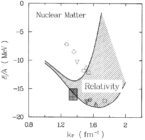
Figure 3: The repulsive relativistic effect in nuclear matter as obtained in a Dirac-Brueckner-Hartree-Fock calculation using Potential B. Saturation points from conventional calculations are displayed in the background (cf. Fig. 1). The checked rectangle represents the empirical value for nuclear matter saturation.

Table 3: Results of a relativistic Dirac-Brueckner calculation in comparison to the corresponding non-relativistic one using Potential B.

	relativistic						non-relativistic
$k_{F}$	${\cal E}/A$	$\tilde{M}/M$	$U_{S}$	$U_{V}$	$\kappa$		${\cal E}/A$	$\tilde{M}/M$	$U_{0}$a	$\kappa$
(fm-1)	(MeV)		(MeV)	(MeV)	(%)		(MeV)		(MeV)	(%)
0.8	–7.02	0.855	–136.2	104.0	23.1		–7.40	0.876	–33.0	26.5
0.9	–8.58	0.814	–174.2	134.1	18.8		–9.02	0.836	–41.0	21.6
1.0	–10.06	0.774	–212.2	164.2	16.1		–10.49	0.797	–49.0	18.5
1.1	–11.18	0.732	–251.3	195.5	12.7		–11.69	0.760	–58.1	14.2
1.2	–12.35	0.691	–290.4	225.8	11.9		–13.21	0.725	–68.5	12.9
1.3	–13.35	0.646	–332.7	259.3	12.5		–14.91	0.687	–80.5	13.1
1.35	–13.55	0.621	–355.9	278.4	13.0		–15.58	0.664	–86.8	13.2
1.4	–13.53	0.601	–374.3	293.4	13.8		–16.43	0.651	–93.2	13.5
1.5	–12.15	0.559	–413.6	328.4	14.4		–17.61	0.618	–106.1	13.0
1.6	–8.46	0.515	–455.2	371.0	15.8		–18.14	0.579	–119.4	12.7
1.7	–1.61	0.477	–491.5	415.1	18.4		–18.25	0.545	–133.2	13.2
1.8	+9.42	0.443	–523.4	463.6	21.9		–17.65	0.489	–147.2	14.3
1.9	25.26	0.418	–546.7	513.5	25.2		–16.41	0.480	–160.7	15.0
2.0	47.56	0.400	–563.6	568.6	27.5		–13.82	0.449	–173.6	15.3
2.1	77.40	0.381	–581.3	640.9	30.2		–9.70	0.411	–186.3	15.7
2.2	114.28	0.370	–591.2	723.5	33.3		–3.82	0.373	–198.1	16.3
As a funtion of the Fermi momentum $k_{F}$, we list: the energy per nucleon ${\cal E}/A$,
$\tilde{M}/M$, the single-particle scalar and vector potentials $U_{S}$ and $U_{V}$, and the wound
integral $\kappa$.
a $U_{0}$ is to be compared to $U_{S}+U_{V}$, cf. Eq. (104).

Table 4: Partial wave contributions to the energy in nuclear matter (in MeV) for a non-relativistic and a relativistic calculation using Potential B.

	$k_{F}=1.1$ fm-1			$k_{F}=1.35$ fm-1			$k_{F}=1.6$ fm-1
State	non-rel.	relativ.		non-rel.	relativ.		non-rel.	relativ.
${}^{1}\!S_{0}$	–10.79	–11.18		–16.01	–16.42		–21.51	–20.36
${}^{3}\!P_{0}$	–2.07	–1.48		–3.74	–1.34		–5.61	+2.17
${}^{1}\!P_{1}$	1.73	1.77		3.25	3.45		5.33	6.08
${}^{3}\!P_{1}$	4.71	5.27		9.77	12.33		17.69	26.65
${}^{3}\!S_{1}$	–15.41	–14.16		–20.10	–17.10		–23.77	–17.03
${}^{3}\!D_{1}$	0.59	0.57		1.38	1.29		2.64	2.25
${}^{1}\!D_{2}$	–0.95	–0.91		–2.28	–2.01		–4.57	–3.39
${}^{3}\!D_{2}$	–1.70	–1.62		–4.00	–3.56		–7.71	–5.99
${}^{3}\!P_{2}$	–3.10	–2.92		–7.06	–6.28		–13.31	–10.73
${}^{3}\!F_{2}$	–0.19	–0.18		–0.54	–0.44		–1.19	–0.67
${}^{1}\!F_{3}$	0.32	0.31		0.80	0.75		1.60	1.40
${}^{3}\!F_{3}$	0.56	0.55		1.51	1.43		3.20	2.87
${}^{3}\!D_{3}$	–0.01	0.00		–0.03	0.00		–0.11	–0.02
${}^{3}\!G_{3}$	0.06	0.06		0.20	0.18		0.49	0.41
$J\geq 4$	–0.34	–0.33		–1.07	–0.98		–2.57	–2.13
Total
potential energy	–26.61	–24.25		–37.93	–28.72		–49.38	–18.51
Kinetic energy	14.91	13.07		22.35	15.16		31.23	10.05
Total energy	–11.69	–11.18		–15.58	–13.55		–18.14	–8.46

Table 5: Energy per particle, ${\cal E}/A$, Fermi momentum, $k_{F}$, and kompression modulus, $K$, at saturation for nuclear matter with and without relativistic effects.

		relativistic				non-relativistic
Potential		${\cal E}/A$	$k_{F}$	K		${\cal E}/A$	$k_{F}$	K
		(MeV)	(fm-1)	(MeV)		(MeV)	(fm-1)	(MeV)
A		–15.59	1.40	290		–23.55	1.85	204
B		–13.60	1.37	249		–18.30	1.66	160
C		–12.26	1.32	185		–15.75	1.54	143

The energy per nucleon in nuclear matter, which is the objective of these calculations, is considered in the nuclear matter rest frame. Thus, the $G$-matrix is needed for the nuclear matter rest frame. Equation (95) gives this nuclear matter $G$-matrix directly in that rest frame. Alternatively, one can calculate the $G$-matrix first in the two-nucleon center-of-mass (c.m.) system (as customary in calculations of the $\cal T$-matrix in two-nucleon scattering), and then perform a Lorentz transformation to the rest frame. This method, which is described in detail in Ref. [42], is, however, complicated, involved, and cumbersome. The advantage of our procedure is that it avoids this complication. Further treatments of Eq. (95) can follow the lines established from conventional Brueckner theory, as e. g.  the use of the angle averaged Pauli projector etc.. Numerically the equation can be solved by standard methodes of momentum space Brueckner calculations [7].

The essential difference to standard Brueckner theory is the use of the potential $\tilde{V}$ in Eq. (95). Indicated by the tilde, this meson-theoretic potential is evaluated by using the spinors of Eq. (92) instead of the free spinors applied in scattering as well as in conventional (’non-relativistic’) Brueckner theory. Since $U_{S}$ (and $\tilde{M}$) are strongly density dependent, so is the potential $\tilde{V}$. $\tilde{M}$ decreases with density. The essential effect in nuclear matter is a suppression of the (attractive) $\sigma$-exchange; this suppression increases with density, providing additional saturation. It turns out (see figures below) that this effect is so strongly density-dependent that the empirical saturation and incompressibility can be reproduced. Furthermore, the prediction for the Landau parameter $f_{0}$ is considerably improved without deteriorating the other parameters (see Table 6 below). Note, that sum rules require $f_{0}>-1$ at nuclear matter density [73].

The single-particle potential

$$U(m)=\frac{\tilde{M}}{\tilde{E_{m}}}\langle m|U|m\rangle=\frac{\tilde{M}}{\tilde{E_{m}}}\langle m|U_{S}+\gamma^{0}U_{V}|m\rangle=\frac{\tilde{M}}{\tilde{E_{m}}}U_{S}+U_{V}$$ (106)

is the self-energy of the nucleon which is defined in terms of the $G$-matrix formally in the usual way

$$U(m)=Re\sum_{n\leq k_{F}}\frac{\tilde{M}^{2}}{\tilde{E_{n}}\tilde{E_{m}}}\langle mn|\tilde{G}(\tilde{z})|mn-nm\rangle$$ (107)

where $m$ denotes a state below or above the Fermi surface (continuous choice). The constants $U_{S}$ and $U_{V}$ are determined from Eqs. (97) and (98). Note that Eq. (91) is an approximation, since the scalar and vector fields are in general momentum dependent; however, it has been shown that this momentum dependence is very weak [38].

The energy per nucleon in nuclear matter is

$$\frac{{\cal E}}{A}=\frac{1}{A}\sum_{m\leq k_{F}}\frac{\tilde{M}}{\tilde{E_{m}}}\langle m|\mbox{\boldmath$\gamma$}\cdot{\bf p}_{m}+M|m\rangle+\frac{1}{2A}\sum_{m,n\leq k_{F}}\frac{\tilde{M}^{2}}{\tilde{E}_{m}\tilde{E}_{n}}\langle mn|\tilde{G}(\tilde{z})|mn-nm\rangle-M\;.$$ (108)

In Eqs. (98) and (99) we use

$$\tilde{z}=\tilde{E}_{m}+\tilde{E}_{n}.$$ (109)

The expression for the energy, Eq. (99), is denoted by the Dirac-Brueckner-Hartree-Fock (DBHF) approximation. If $\tilde{M}$ is replaced by $M$, we will speak of the Brueckner-Hartree-Fock (BHF) approximation, since this case, qualitatively and quantitatively, corresponds to conventional non-relativistic Brueckner theory. Thus, we will occasionally denote the DBHF calculation by ‘relativistic’ and the BHF calculation by ‘non-relativistic’ (though, strictly speaking, all our calculations are relativistic).

In Equations. (97-99) the states $|m\rangle$ and $|n\rangle$ are represented by Dirac spinors of the kind Eq. (92) and an appropriate isospin wavefunction, $\langle m|$ and $\langle n|$ are the adjoint Dirac spinors $\bar{\tilde{u}}=\tilde{u}^{\dagger}\gamma^{0}$ with $\bar{\tilde{u}}\tilde{u}=1$; $\tilde{E_{m}}\equiv\sqrt{\tilde{M}^{2}+{\bf p}^{2}_{m}}$. The states of the nucleons in nuclear matter, $w$, are to be normalized by $w^{\dagger}w=1$. This is achieved by defining $w\equiv\sqrt{\tilde{M}/\tilde{E}}\times\tilde{u}$ which explains factors of $\tilde{M}/\tilde{E}$ in Eqs. (97-99).

The first term on the r.h.s. of Eq. (99) — the ‘kinetic energy’ — is in more explicit form

$$\frac{1}{A}\sum_{m\leq k_{F}}\frac{M\tilde{M}+{\bf p}_{m}^{2}}{\tilde{E_{m}}}.$$ (110)

The single particle energy is

$$\epsilon_{m} = \frac{\tilde{M}}{\tilde{E_{m}}}\langle m|\mbox{\boldmath$\gamma$}\cdot{\bf p}_{m}+M|m\rangle+U(m)$$ (111)

$$= \tilde{E_{m}}+U_{V}$$ (112)

$$= \tilde{E_{m}}-\tilde{M}+M+U_{0}.$$ (113)

5 Results for Nuclear Matter

Table 6: Landau parameters at various densities from a non-relativistic and a relativistic nuclear matter calculation using Potential B.

$k_{F}$
(fm-1)	density		$f_{0}$	$f_{0}^{\prime}$	$g_{0}$	$g_{0}^{\prime}$
1.0	$0.4\rho_{0}$	relativistic	–1.37	0.57	0.22	0.66
		non-relativisic	–1.50	0.62	0.16	0.66
1.35	$\rho_{0}$	relativistic	–0.79	0.35	0.28	0.67
		non-relativisic	–1.27	0.38	0.15	0.67
1.7	$2\rho_{0}$	relativistic	0.56	0.29	0.36	0.68
		non-relativisic	–0.99	0.20	0.14	0.69
2.0	$3.25\rho_{0}$	relativistic	2.21	0.37	0.38	0.69
		non-relativisic	–0.71	0.09	0.11	0.71
(empirical)			($0\pm 0.2$)	($\approx 0.8$)	($\approx 0.2$)	($\approx 0.9$)

Table 7: Nuclear matter results of a relativistic Dirac-Brueckner calculation applying Potential A. Notation as in Table 3.

	relativistic						non-relativistic
$k_{F}$	${\cal E}/A$	$\tilde{M}/M$	$U_{S}$	$U_{V}$	$\kappa$		${\cal E}/A$
(fm-1)	(MeV)		(MeV)	(MeV)	(%)		(MeV)
0.8	–7.27	0.857	–134.3	101.6	22.6		–7.60
0.9	–8.97	0.817	–172.1	131.1	18.1		–9.38
1.0	–10.62	0.777	–209.8	160.6	15.2		–11.01
1.1	–11.96	0.736	–248.5	191.1	11.5		–12.44
1.2	–13.44	0.692	–288.8	222.0	10.6		–14.24
1.3	–14.86	0.647	–331.6	255.0	11.0		–16.35
1.35	–15.32	0.621	–355.7	274.7	11.5		–17.28
1.4	–15.59	0.601	–374.9	289.8	12.1		–18.41
1.5	–14.88	0.557	–416.3	325.7	12.7		–20.25
1.6	–11.96	0.511	–459.6	368.6	14.2		–21.64
1.7	–5.88	0.470	–497.2	412.8	16.9		–22.76
1.8	+4.44	0.435	–530.4	461.6	20.4		–23.38
1.9	19.72	0.409	–554.8	512.0	23.7		–23.54
2.0	41.62	0.390	–572.4	567.5	26.3		–22.60
2.1	71.20	0.371	–590.2	640.3	29.1		–20.42
2.2	106.52	0.366	–595.0	732.5	31.9		–16.74

Table 8: Nuclear matter results of a relativistic Dirac-Brueckner calculation applying Potential C. Notation as in Table 3.

	relativistic						non-relativistic
$k_{F}$	${\cal E}/A$	$\tilde{M}/M$	$U_{S}$	$U_{V}$	$\kappa$		${\cal E}/A$
(fm-1)	(MeV)		(MeV)	(MeV)	(%)		(MeV)
0.8	–6.80	0.851	–140.3	108.6	23.0		–7.21
0.9	–8.30	0.812	–176.6	137.2	19.1		–8.79
1.0	–9.69	0.773	–212.9	165.8	16.9		–10.20
1.1	–10.64	0.732	–252.1	197.5	13.6		–11.15
1.2	–11.57	0.688	–292.8	229.8	13.0		–12.46
1.3	–12.25	0.644	–334.0	262.8	13.8		–13.87
1.35	–12.24	0.620	–356.6	281.8	14.5		–14.35
1.4	–11.99	0.601	–374.2	296.4	15.3		–15.02
1.5	–10.06	0.561	–411.8	330.9	16.0		–15.73
1.6	–5.72	0.519	–451.7	373.2	17.5		–15.65
1.7	+1.81	0.482	–486.3	416.6	20.2		–15.01
1.8	13.50	0.450	–516.8	464.6	23.7		–13.50
1.9	29.85	0.426	–538.8	513.8	26.9		–11.22
2.0	52.48	0.409	–554.6	567.7	29.2		–7.39
2.1	82.54	0.391	–571.8	639.4	31.8		–1.75
2.2	119.89	0.379	–583.0	717.7	34.9		+5.88

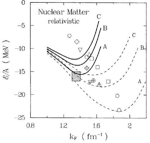
Figure 4: Results from calculations with a family of relativistic potentials revealing a new Coester band which meets the empirical area; solid lines: relativistic, dashed lines: non-relativistic calculations. For comparison, saturation points from conventional calculations are displayed in the background (cf. Fig. 1). The shaded square denotes the empirical value for nuclear matter saturation.

We apply now the three OBE potentials presented in Sect. 3.3 to nuclear matter. We stress again, that our potentials use for $\pi NN$ the coupling of derivative (pseudovector) type. This is improtant because the pseudoscalar $\pi NN$ coupling leads to an unrealistcally large attractive medium effect [38].

The main difference between the three potentials applied here, is the strength of the tensor force as reflected in the predicted D-state probability of the deuteron, $P_{D}$. With $P_{D}=4.5\%$, Potential A has the weakest tensor force. Potential B and C predict 5.1% and 5.5%, respectively (cf. Table 2). It is well-known [10] that the strength of the tensor force determines the location of the nuclear matter saturation point on the Coester band [22]. To find out the structure of the Coester band, predictions from more than one potential are needed.

All results presented in this section are obtained either in the Bruckner-Hartree-Fock (BHF) or the Dirac-Brueckner-Hartree-Fock (DBHF) approximation; as mentioned before, occasionally, we will denote these two methods also as the ‘non-relativistic’ and the ‘relativistic’ calculation, respectively.

The repulsive relativistic effect in nuclear matter as created by the DBHF method in shown in Fig. 3. In addition, in Table 3, we list the following quantities as a function of the Fermi momentum $k_{F}$: the energy per nucleon, ${\cal E}/A$, the ratio $\tilde{M}/M$, the single-particle scalar and vector potentials $U_{S}$ and $U_{V}$, and the wound integral $\kappa$. (For the definition of $\kappa$ and for explicit formulae appropriate for the momentum-space framework, see section 5 of Ref. [7].) $\kappa$ can be understood as the expansion parameter for the hole-line series.

As mentioned in Sect. 4, the suppression of the $\sigma$ contribution can be understood in simple terms by considering the covariant one-$\sigma$-exchange amplitude, for ${\bf q^{\prime}}={\bf q}$ and $\lambda_{i}=\lambda_{i}^{\prime}$ (as used in the Hartree approximation), in which case, due to the covariant normalization of the Dirac spinors, the numerator becomes ${\bf 1}$. Since the physical states of the nucleons in nuclear matter, $w$, are to be normalized by $w^{\dagger}w=1$ implying $w\equiv\sqrt{\tilde{M}/\tilde{E}}\times\tilde{u}$, the sigma (as any other) contribution gets the (scalar density) factor $(\tilde{M}/\tilde{E})^{2}$ (see second term on the r.h.s. of Eq. (99)) which decreases with decreasing $\tilde{M}$ (i. e. increasing density). A corresponding consideration for the time-like ($\gamma_{0}$) component of $\omega$-exchange would lead to no changes for that contribution. However, due to the exchange term and correlations there is a small enhancement of the repulsion created by the $\omega$ with density.

¿From the numbers given in Table 3 it is seen that the relativistic effect on the energy per nucleon, $\Delta({\cal E}/A)_{rel}$ (i. e. the difference between the relativistic and non-relativistic calculation), is well fitted by the ansatz

$$\Delta({\cal E}/A)_{rel}\approx 2\mbox{ MeV}\times(\rho/\rho_{0})^{8/3},$$ (114)

which is suggested by an estimate by Keister and Wiringa [74].

Furthermore, Table 3 shows that up to nuclear matter density the wound integral $\kappa$ is slightly smaller for the relativistic approach than for the non-relativistic one. This implies that in this region the relativistic many-body scheme should be slightly better convergent. Beyond nuclear matter density, the situation is reversed. In addition, it is amusing to note that for all values of $k_{F}$ the ratio $\tilde{M}/M$ is almost the same for the non-relativistic and the relativistic approach. Low values for $\tilde{M}/M$ have often been critizised. However, they are not a consequence of the relativistic approach but are due to the Brueckner-Hartree-Fock approximation. Higher order corrections will enhance this quantity. For a recent discussion of the effective mass in relativistic and non-relativistic approaches see Refs. [75, 76].

The representation of nucleons by Dirac spinors with an effective mass, $\tilde{M}$, can be interpreted, as taking virtual nucleon-antinucleon excitations in the many-body environment (many-body Z-graphs) effectively into account [77]. This can be made plausible by expanding the spinors Eq. (92) in terms of (a complete set of) spinor solutions of the free Dirac equation which will necessarily also include solutions representing negative energy (antiparticle) states [35].

In Table 4, we compare the contributions in various partial-wave states as obtained in a relativistic calculation to that from the corresponding non-relativistic one. Detailed investigations have shown that the repulsive relativistic effect seen in that table for the $P$-wave contributions is essentially due to $\sigma$ suppression together with a signature of spin-orbit force enhancement. The change of the ${}^{1}\!S_{0}$ contribution is so small, because of a cancelation of effects due to $\sigma$ and $\rho$. Apart from $\sigma$ reduction, the repulsive effect in ${}^{3}\!S_{1}$ is due to a suppression of the twice iterated one-pion exchange for reasons quite analogous to the sigma suppression.

A comparison between relativistic and non-relativistic Brueckner-Hartree-Fock calculations for all three potentials is shown in Fig. 4. For the non- relativistic approach, the three saturation points are clearly on the Coester band. However, using the relativistic method, the saturation points are located on a new band which is shifted towards lower Fermi momenta (densities) and even meets the empirical area. This is a very desirable effect. The reason for this shift of the Coester band is the additional strongly density dependent repulsion which the relativistic approach gives rise to. In Table 5, the saturation points for the different potentials are given for the relativistic as well as the non-relativistic calculation. In the relativistic case, the incompressibility of nuclear matter using Potential B is about 250 MeV which is in satisfactory agreement with the empirical value of $210\pm 30$ MeV [78]. Note that in the relativistic Walecka model, 540 MeV is obtained for the compression modulus [31].

For completeness, we present in Table 6 the Landau parameters at various densities as obtained in a relativistic as well as a non-relativistic nuclear matter calculation. Based on the nuclear matter G-matrix, the effective particle-hole interaction at the Fermi surface is calculated and, multiplied by the density of states $k_{F}M/(\hbar^{2}\pi^{2})$, parametrized by: $F=f+f^{\prime}\tau_{1}\cdot\tau_{2}+g\sigma_{1}\cdot\sigma_{2}+g^{\prime}\sigma_{1}\cdot\sigma_{2}\tau_{1}\cdot\tau_{2}$. ¿From an expansion of the parameters in terms of Legendre polynominals, $P_{l}$, we give in Table 6 the coefficient for $l=0$. For more details and the empirical values see Ref. [79]. Notice that the prediction for the Landau parameter $f_{0}$ is considerably improved in the relativistic calculation without deteriorating the other parameters. Sum rules require $f_{0}>-1$ at nuclear matter density [73]. Finally, Tables 7 and 8 contain more results for Potentials A and C.

Concerning nuclear matter at higher densities and neutron matter, we like to refer the interested reader to Ref. [76].

6 In-Medium NN Cross Sections

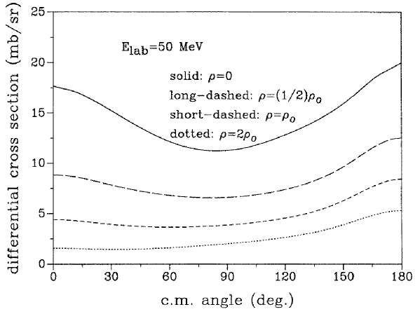
Figure 5: In-medium $np$ differential cross sections at 50 MeV laboratory kinetic energy, as obtained for various densities.

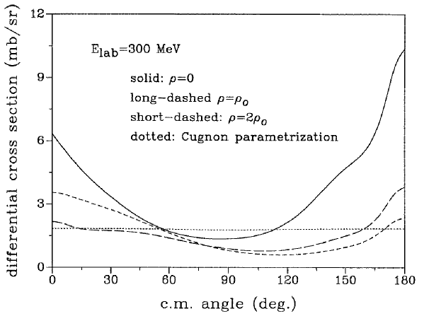
Figure 6: In-medium $np$ differential cross sections at 300 MeV laboratory kinetic energy, as obtained for various densities using the Bonn A potential (solid, long-dashed, and short-dashed lines). The dotted line shows the parametrisation by Cugnon et al. [92].

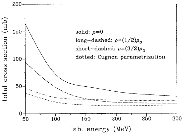
Figure 7: In-medium $np$ total cross sections as obtained for various densities using the Bonn A potential (solid, long-dashed, and short-dashed lines). The dotted line shows the parametrisation by Cugnon et al. [92].

The investigation of in-medium NN scattering is of interest for intermediate-energy heavy-ion reactions. Experimentally, nucleus-nucleus collisions at intermediate energies provide a unique opportunity to form a piece of nuclear matter in the laboratory with a density up to 2-3$\rho_{0}$ (with $\rho_{0}$, in the range of 0.15 to 0.19 fm^-3, the saturation density of normal nuclear matter; in this section we use $\rho_{0}$=0.18 fm^-3) [80, 81]. Thus it is possible to study the properties of hadrons in a dense medium. Since this piece of dense nuclear matter exists only for a very short time (typically $10^{-23}$ -$10^{-22}$ s), it is necessary to use transport models to simulate the entire collision process and to deduce the properties of the intermediate stage from the known initial conditions and the final-state observables. At intermediate energies, both the mean field and the two-body collisions play an equally important role in the dynamical evolution of the colliding system; they have to be taken into account in the transport models on an equal footing, together with a proper treatment of the Pauli blocking for the in-medium two-body collisions. The Boltzmann-Uehling-Uhlenbeck (BUU) equation [82, 83] and quantum molecular dynamics (QMD) [84, 85], as well as their relativistic extensions (RBUU and RQMD) [86, 87, 88, 89], are promising transport models for the description of intermediate-energy heavy-ion reactions. In addition to the mean field [90], the in-medium NN cross sections are also important ingredients of these transport models. Specifically, in-medium total as well as differential NN cross sections are needed by these models in dealing with the in-medium NN scattering using a Monte Carlo method.

In this section, we will calculate the elastic in-medium NN cross sections in a microscopic way. We base our investigation on the Bonn potentials presented in Sect. 3 and the Dirac-Brueckner approach explained in Sect. 4. The original, detailed paper on this subject is Ref. [91].

In-medium NN cross sections can be calculated from the in-medium $\tilde{G}$ matrix. Here, we evaluate the $\tilde{G}$-matrix in the center-of-mass (c.m.) frame of the two interacting nucleons, i. e., we use Eq. (95) with ${\bf P}=0$. For the starting energy, Eq. (96), we have now: $\tilde{z}=2\tilde{E}_{q}=2\sqrt{\tilde{m}^{2}+q^{2}}$, where $q$ is related to the kinetic energy of the incident nucleon in the “laboratory system” ($E_{lab}$), in which the other nucleon is at rest, by: $E_{lab}=2q^{2}/m$. Thus, we consider two colliding nucleons in nuclear matter. The Pauli projector is represented by one Fermi sphere as in conventional nuclear matter calculations. This Pauli-projector, which is originally defined in the nuclear matter rest frame, must be boosted to the c.m. frame of the two interacting nucleons. For a detailed discussion of this and the explicit formulae, see Refs. [40, 42].

In Fig. 5 we show the results for the in-medium $np$ differential cross sections as a function of the c.m. angle at $E_{lab}$=50 MeV and in Fig. 6 at 300 MeV. We consider the medium densities $\rho$=0 (free-space scattering), (1/2)$\rho_{0}$, $\rho_{0}$, and $2\rho_{0}$. The results are obtained by using the Bonn A potential. At low incident energies (Fig. 5), the $np$ differential cross section always decreases with increasing density, at both forward and backward angles. At high incident energies (Fig. 6), the np differential cross section for forward angles decreases when going from $\rho$=0 to $\rho_{0}$ and then increases for higher densities. The differential cross section at backward angles always decreases with density. While the free np differential cross sections are highly anisotropic, the in-medium cross sections become more isotropic with increasing density.

We have also calculated the in-medium cross sections using other potentials (Bonn B and C) and found very little difference as compared to Bonn A. Thus, there is fortunately little model dependence in our predictions.

It is also interesting to compare the results obtained in this work with the parametrized NN cross sections proposed by Cugnon et al. [82, 92] which are often used in transport models such as BUU and QMD. This comparison is included in Fig. 6. It is clearly seen that, while the Cugnon parametrization is almost isotropic, the microscopic results still have some anisotropy at all densities considered. The anisotropy in the present results decreases with increasing density. There is also density dependence in the microscopic differential cross section, while the Cugnon parametrization is density independent.

We mention that Cugnon et al. [92] have parametrized the free $pp$ cross sections. This explains the almost-isotropy in their differential cross sections as well as the lack of the density dependence. Note that in the work of Cugnon et al., [92], no difference is made between proton and neutron; thus, the $pp$ cross sections are also used for $np$ scattering. There are, however, well-known differences between $pp$ and $np$ cross sections which in the more accurate microscopic calculations of the near future may be relevant. The difference between the (in-medium) $np$ and $pp$ cross sections is discussed in detail in Ref. [93]. In this section, we restrict our discussion of “NN cross sections” to $np$ cross sections.

The np differential cross section in free space can be well parametrized by the following simple expression:

$${d\sigma\over d\Omega}(E_{lab},\theta)={17.42\over 1.0+0.05(E_{lab}^{0.7}-15.5)}exp[b(cos^{2}\theta+sin^{2}{\theta\over 7}-1.0)]$$ (115)

with

$$b=0.0008(E_{lab}^{0.54}-4.625)~{}{\rm for}~{}~{}E_{lab}\leq 100{\rm MeV}$$

and

$$b=0.0006(36.65-E_{lab}^{0.58})~{}{\rm for}~{}~{}E_{lab}>100{\rm MeV}.$$

with $E_{lab}$ in the units of MeV.

It would be useful to parametrize the in-medium $np$ differential cross section as well. However, the complicated dependence of the in-medium differential cross sections on angles, energy, and especially density makes this very difficult. Instead, we have prepared a data file, containing in-medium differential cross section as a function of angle for a number of densities and energies, from which the differential cross sections for all densities in the range 0-3$\rho_{0}$ and all energies in the range 0-300 MeV can be interpolated. This data file is available from one of the authors (R. M.) upon request.

In addition to the in-medium NN differential cross sections which enter the transport models to determine the direction of the outgoing nucleons, the in-medium total NN cross sections, $\sigma_{NN}$, are also of interest. They provide a criterion for whether a pair of nucleons will collide or not by comparing their closest distance to $\sqrt{\sigma_{NN}/\pi}$. We show in Fig. 7 the in-medium total cross sections as function of the incident energy $E_{lab}$ and density. It is seen that the in-medium total cross sections decrease substantially with increasing density, particularly for low incident energies.

Figure 7 also includes a comparison with the total cross sections used by Cugnon et al. [82, 92] (dotted line in Fig. 7). It is seen that at low energies and low densities, the Cugnon parametrization underestimates the microscopic results, while at higher energies and higher density it is the other way around. Note that the Cugnon parametrization is not density dependent, and, thus, predicts the same for all densities.

Finally, we propose a parametrization for the total $np$ cross section as a function of the incident energy $E_{lab}$ and density $\rho$

$$\sigma_{np}(E_{lab},\rho)=(31.5+0.092{\rm abs}(20.2-E_{lab}^{0.53})^{2.9}){1.0+0.0034E_{lab}^{1.51}\rho^{2}\over 1.0+21.55\rho^{1.34}}$$ (116)

where $E_{lab}$ and $\rho$ are in the units of MeV and fm^-3, respectively.

The major conclusions of the present microscopic calculations are:

• There is strong density dependence for the in-medium cross sections. With the increase of density, the cross sections decrease. This indicates that a proper treatment of the density-dependence of the in-medium NN cross sections is important.

• Our microscopic predictions differ from the commonly used parametrizations of the differential and the total cross sections developed by Cugnon et al. [82, 92]. The Cugnon parametrization underestimates the anisotropy of the in-medium np differential cross sections. In the case of the total cross sections, the Cugnon parametrization either underestimates or overestimates the microscopic results, depending on energy and density.

More details of this investigation can be found in Refs. [91, 93].

7 Finite Nuclei

Encouraged by the good results for nuclear matter, one may now try to describe finite nuclei starting from the free-space nucleon-nucleon interaction. A straightforward way would be to solve the relativistic Brueckner-Hartree-Fock equations for finite systems. This is, however, an extremely difficult task [55, 98]. Therefore, it might be a reasonable next step to incorporate the DBHF results in a relativistic Hartree framework where the coupling constants are made density dependent so as to reproduce the nuclear matter results. This relativistic density dependent Hartree (RDDH) approach is similar in spirit to the work by Negele in the nonrelativistic approach [95].

The working basis of the RDDH approach for finite nuclei is the relativistic Hartree Lagrangian [29] (sigma-omega model Lagrangian of Walecka [34]). Writing explicitly the density dependence of the coupling constants,we have

$$\cal{L}_{\hbox{\scriptsize RDDH}} = \bar{\psi}\left(i\gamma_{\mu}\partial^{\mu}-M-g_{\sigma}(\rho)\sigma-g_{\omega}(\rho)\gamma_{\mu}\omega^{\mu}\right)\psi$$ (117)

$$+\frac{1}{2}\left(\partial^{\mu}\sigma\right)^{2}-\frac{1}{2}m_{\sigma}^{2}\sigma^{2}-\frac{1}{4}\left(\partial_{\mu}\omega_{\nu}-\partial_{\nu}\omega_{\mu}\right)^{2}+\frac{1}{2}m_{\omega}^{2}\omega_{\mu}^{2}\;,$$

in conventional notation [48]. In Hartree approximation (mean field approximation), the nucleon self-energy in nuclear matter is given by

$$\Sigma_{\hbox{\scriptsize RDDH}}(\rho) = \hbox{U}_{s}(\rho)+\hbox{U}_{v}(\rho)\gamma_{0}\;.$$ (118)

Here, the scalar and the vector potentials are expressed in terms of the coupling constants g${}_{\sigma}(\rho)$ and g${}_{\omega}(\rho)$ through

$$\hbox{U}_{s}(\rho) = -\frac{{g_{\sigma}}^{2}(\rho)}{m_{\sigma}^{2}}\rho_{s}$$

$$\hbox{U}_{v}(\rho) = \frac{{g_{\omega}}^{2}(\rho)}{m_{\omega}^{2}}\rho_{v}\;,$$ (119)

where $\rho_{s}$ and $\rho_{v}$ are the scalar and the vector densities, respectively:

$$\rho_{s} = <\bar{\psi}\psi>\;=\;4\int\limits_{0}^{k_{\hbox{\scriptsize F}}}\frac{d^{3}k}{(2\pi)^{3}}\,\frac{M^{*}}{E^{*}}\;,$$

$$\rho_{v} = <\bar{\psi}\gamma_{0}\psi>\;=\;4\int\limits_{0}^{k_{\hbox{\scriptsize F}}}\frac{d^{3}k}{(2\pi)^{3}}\;.$$ (120)

The scalar potential is related to the effective mass by $M^{*}\,=\,M+\hbox{U}_{s}(\rho)$. The connection of the RDDH approach to the DBHF theory is made through the nucleon self-energy in nuclear matter, Eq. (109). In fact, one can express the DBHF self-energy in nuclear matter in this form [37] using the symmetry requirements and redefinition of various terms through the use of the Dirac equation [96]. The density dependent coupling constants are then obtained through Eqs. (110) and (111), where U${}_{s}(\rho)$ and U${}_{v}(\rho)$ are the results of the DBHF calculations of nuclear matter.

We write the equations of motion for finite nuclei for completeness. The normal modes of the nucleon are calculated with the Dirac equation,

$$\left(-i\mbox{\boldmath$\alpha\cdot\nabla$}+\beta M^{*}(r)+V(r)\right)\psi_{i}({\bf r}) = E_{i}\psi_{i}({\bf r})$$ (121)

with $M^{*}(r)\,=\,M+g_{\sigma}(r)\sigma(r)$ and $\hbox{V}(r)\,=\,g_{\omega}(r)\omega^{0}(r)+e\frac{1-\tau_{3}}{2}A^{0}(r)$.

The Klein-Gordon equations for $\sigma$, $\omega^{0}$, and $A^{0}$ are

$$\left(-\triangle+m_{\sigma}^{2}\right)\sigma(r) = -g_{\sigma}(r)\rho_{s}(r)$$

$$\left(-\triangle+m_{\omega}^{2}\right)\omega^{0}(r) = g_{\omega}(r)\rho_{v}(r)$$

$$-\triangle A^{0}(r) = e\rho_{p}(r),$$ (122)

where $\rho_{s}$, $\rho_{v}$ and $\rho_{p}$ are the scalar, vector and proton densities, respectively, which are obtained through the Dirac wavefunctions. We solve the coupled differential equations self-consistently. The center of mass corrections are applied in the same way as in Ref. [97].

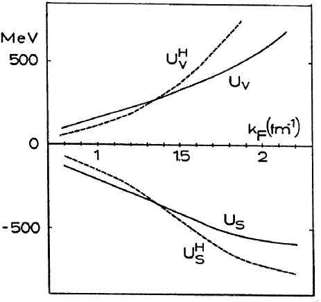
Figure 8: Vector and scalar potentials for relativistic density dependent Hartree (full lines) and relativistic Hartree only (dashed lines) as a function of k_F.

In Fig. 8, the vector and the scalar potentials, U_v and U_s are depicted as a function of k_F. At normal matter density, k_F = 1.35 fm^-1, U_v = 274.7 MeV and U_s = –355.7 MeV. As a comparison, the vector and scalar mean-field potentials are shown using constant (density independent) couplings; i.e. the scalar and vector potential parameters are the ones of Potential A. This comparison clearly indicates that one needs density dependent coupling constants in order to reproduce the nuclear matter results within the relativistic Hartree framework.

Now we fit the coupling constants g${}_{\sigma}(\rho)$ and g${}_{\omega}(\rho)$ to the self-energies U_s and U_v with the choice that m_σ and m_ω are the masses in Potential A as a standard choice; m_σ = 550 MeV and m_ω = 782.6 MeV. As can be seen from Eq. (110), the relevant quantities are g${}_{\sigma}^{2}$ and g${}_{\omega}^{2}$. At k_F = 0.8, 1.1, 1.5 we obtain g${}_{\sigma}^{2}$/4$\pi$ = 12.3, 8.91, 6.23 and g${}_{\omega}^{2}$/4$\pi$ = 18.63, 13.48, 9.06, respectively. This shows that the coupling constants at the surface are more than 40% bigger than in the interior. At nuclear matter density (k_F = 1.35fm${}^{-}1$) the coupling constants are not modified as one can see from Fig. 8. But at smaller densities both coupling constants are growing. We note here that U_s and U_v are, in principle, dependent not only on the density but also on the momentum of the nucleon. We neglect this weak momentum dependence in our study of finite nuclei.

We calculate ¹⁶O and ⁴⁰Ca as examples for finite nuclei within the RDDH approach. The calculated results on the binding energies, single particle energies and charge radii (using the Bonn A potential) are tabulated in Table 9. For comparison, results of nonrelativistic Brueckner-Hartree-Fock calculations for ¹⁶O with the same potential (Bonn A) are shown in the column N-BHF [98]. It is interesting to find that the RDDH results are very close to experiment. The improvements, as compared to N-BHF, are remarkable. The root mean square charge radius is almost perfect, while the binding energy is slightly smaller than experiment. If we compare relativistic and nonrelativistic results, we find that the radius of the relativistic calculation is larger. This is natural since, e. g., the lower component of the relativistic 1p3/2 - wavefunction looks like a nonrelativistic 1d3/2 - wavefuction. This shifts part of the density to the surface and leads to a larger radius in the relativistic case. This has also consequences for the binding energy per nucleon. Using the Bethe-Weizsaecker mass formula, we can estimate that surface and Coulomb effects lead to 2 to 3 MeV less repulsion for the relativistic calculation since the radius is larger. Although the volume effect is 1 to 2 MeV more repulsive in the relativistic case which has been determined in nuclear matter in Ref. [39], the relativistic description of finite nuclei yields altogether more binding energy per nucleon. This shows that relativistic effects lead off the Coester band, which exists for finite nuclei, too.

Table 9: The binding energy per nucleon, root-mean-square charge radius and single particle energies are displayed for the relativistic density dependent Hartree(RDDH) approach, the nonrelativistic Brueckner-Hartree-Fock(N–BHF) method and experiment, respectively. The Bonn A potential is used. The upper part of the table is for ¹⁶O and the lower one for ⁴⁰Ca.

${}^{16}O$	RDDH	N–BHF	Experiment
BE/A [MeV]	–7.5	–5.95	–7.98
rc [fm]	2.66	2.31	$2.70\pm 0.05$
$\epsilon$(1s1/2) [MeV]	–43.5	–56.6	$-40\pm 8$
$\epsilon$(1p3/2) [MeV]	–21.8	–25.7	–18.4
$\epsilon$(1p1/2) [MeV]	–16.5	–17.4	–12.1

${}^{40}Ca$	RDDH	N–BHF	Experiment
BE/A [MeV]	–8.0	–8.29	–8.5
rc [fm]	3.36	2.64	3.5
$\epsilon$(1s1/2) [MeV]	–53.3	–	$-50\pm 8$
$\epsilon$(1p3/2) [MeV]	–36.0	–	$-34\pm 5$
$\epsilon$(1p1/2) [MeV]	–32.5	–	$-34\pm 5$
$\epsilon$(1d5/2) [MeV]	–19.3	–30.2	$-14\pm 2$
$\epsilon$(2s1/2) [MeV]	–14.3	–24.5	$-10\pm 1$
$\epsilon$(1d3/2) [MeV]	–13.6	–16.5	$-7\pm 1$

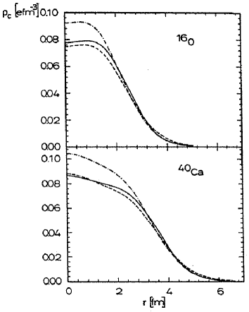
Figure 9: Comparison of the densities in relativistic density dependent Hartree and experiment for ¹⁶O and ⁴⁰Ca, respectively. The results with the Bonn A potential are shown by the dash-dotted curve, while the corresponding ones for Bonn C are depicted by the dashed one.

In Fig. 9, we show a comparison with experimental charge density distributions obtained from elastic electron scattering [97]. The RDDH results with the Bonn A potential (dash-dotted curve) compare fairly well with the experimental data. Looking more closely, the central density comes out to be higher than experiment and the density falls off slightly faster than experiment. This observation of the density and the slightly smaller binding discussed above, seems to be the reflection of the equation of state of nuclear matter as shown in Fig. 4. In fact, when we take the DBHF results from the Bonn C potential, whose saturation density is almost perfect but the saturation energy is about 4 MeV above the experimental value, the charge density distributions are found to be very good as can be seen in Fig. 9 (dashed curve). In this case, however, the binding energies of finite nuclei are found to be too small; i.e. E/A = - 5.9 MeV for ¹⁶O and E/A = - 6.0 MeV for ⁴⁰Ca.

Another issue is the density-dependence of meson masses; this is discussed in Ref. [99].

8 Summary and Outlook

In this chapter we have presented the formalism for a relativistic approach to two-nucleon scattering and nuclear structure. The latter is based upon a relativistic extension of Brueckner theory. The essential idea of this approach is to use the Dirac equation for the single particle motion. The nucleon self-energy in nuclear matter obtained in this framework consists of a large (attractive) scalar and (repulsive) vector field. The size of these potentials (several hundred MeV) motivates the use of the Dirac equation.

Furthermore, we have applied relativistic meson-exchange potentials appropriate for this approach. The one-boson-exchange (OBE) model includes the six non-strange bosons with masses below 1 GeV/c², $\pi,\eta,\sigma,\delta,\omega,$ and $\rho$. The potentials describe low energy NN scattering and the properties of the deuteron quantitatively. Thus, they are suitable for (parameter-free) microscopic nuclear structure calculations. Apart from the usual interaction Lagrangians for heavy mesons, these potentials apply the pseudovector (gradient) coupling for the $\pi NN$ (and $\eta NN$) vertex. For a relativistic approach, it is necessary to apply this coupling for the pseudoscalar mesons, since the commonly used pseudoscalar coupling leads to unrealistically attractive contributions. This has its origin in chiral symmetry.

The consideration of the two-nucleon system is based upon the relativistic three-dimensional reduction of the Bethe-Salpeter equation introduced by Thompson. We derive and present the Thompson equation for an arbitrary frame. In two-nucleon scattering, this equation is applied in the two-nucleon c.m. system, while in nuclear matter, the nuclear matter rest frame is used. Thus, we calculate the nuclear matter $G$-matrix directly in the nuclear matter rest frame in which it is needed to obtain the energy of the many-body system. The advantage of this method is that, in the nuclear medium, the rather involved and tedious transformation between the two-nucleon c.m. frame and the nuclear matter rest frame is avoided.

Using the framework outlined, the properties of nuclear matter are calculated in the Dirac-Brueckner-Hartree-Fock (DBHF) approximation. The single particle scalar and vector fields as well as the single particle wave functions (Dirac spinors) are determined fully self-consistently. The strong attractive scalar field leads to a reduction of the nucleon mass in the medium, which increases with density. One consequence of this is a suppression of the (attractive) scalar-boson exchange. This strongly density-dependent effect improves nuclear saturation considerably such that the empirical saturation energy and density can be explained correctly. Our calculations include also the saturation mechanisms of conventional (non-relativistic) many-body theory (i. e. Pauli and dispersion effects). The predictions for the compression modulus of nuclear matter as well as the Landau parameters are in satisfactory agreement with empirical information.

In spite of the success of the present calculations, several critical questions can be raised. First, there will be contributions of higher order in the conventional hole-line expansion. For non-relativistic Brueckner theory, Day found an increase in the binding energy per nucleon of 5–7 MeV from the three- and four-hole line contributions. Note that in the work of Day the standard choice (‘gap’ choice) for the single-particle potential is used (this is true for all results displayed in Table 1 and Fig. 1).. However, in the calculations of our work the continuous choice for the single-particle potential, Eq. (98), is applied. In the two-hole line approximation, this choice leads to about 4 MeV more binding energy per nucleon as compared to the gap choice. Investigations by the Liège group [100] suggest that a lowest order calculation with the continuous choice effectively includes the three-hole line contributions. In the light of this result, the contributions of higher order in the hole-line expansion, missing in our work, may be believed to be small.

In a recent study, a special class of ring-diagrams has been summed up to infinite orders using our relativistic G-matrix. Only a minor change of the present DBHF result is found [101] which, however, further improves the saturation density.

Secondly, one may question the OBE model. The weakest part of that model is the scalar isoscalar $\sigma$ boson. However, as mentioned, Dirac-Brueckner calculations have also been performed with more realistic meson models, in which the fictitious $\sigma$ is replaced by an explicit description of the $2\pi$-exchange contribution to the NN interaction. In those calculations, it is found that the relativistic effect comes out almost exactly the same as in the OBE model [43]. This is not too surprising since it has been known for a long time that the $2\pi$-exchange part of the nuclear potential is well approximated by the exchange of a single scalar isoscalar boson of intermediate mass.

One may also criticize that the present approach is restricted to positive-energy nucleons. At a first glance, this may appear rather inconsistent in a relativistic framework. However, calculations done for two-nucleon scattering have shown that the contributions from virtual anti-nucleon intermediate states (pair-terms) are extremely small (when the pseudovector coupling is used for the pion) [49, 50]. Thus, the medium effects on this small contributions will be even smaller. This has been confirmed by the relativistic $G$-matrix calculations including antiparticle intermediate states by Amorim and Tjon [102].

Since higher orders in the hole-line expansion are attractive, while corrections from the Dirac sea (of anti-nucleons) have (as far as calculations exist) yielded additional repulsion [42], cancelations may occur between many-body contributions missing in the present approach. Thus, it is not unlikely that DBHF may ultimately turn out to be a reasonable approximation to this very complex (relativistic) many-body problem.

We have also calculated cross sections for NN scattering in the nuclear medium. We find strong density dependence for the in-medium cross sections. The results from our microscopic derivation differ substantially from simple cross section parametrizations that are commonly used in heavy ion reaction calculations. Our in-medium cross sections together with our momentum-dependent mean field [90], which are both derived on an equal footing, can now be used as input for consistent transport model calculations of heavy ion reactions.

Moreover, we developed a relativistic density-dependent Hartree approach for finite nuclei, where the coupling constants of the relativistic Hartree-Lagrangian are made density-dependent and are obtained from the relativistic Brueckner-Hartree-Fock results of nuclear matter. The results on binding energies and root-mean-square radii of ¹⁶O and ⁴⁰Ca agree very well with experiment.

Further applications of our approach to the nucleon mean free path and proton-nucleus scattering are presented in Refs. [103, 104].

On a more fundamental level, one may raise the critical question how serious and reliable the meson model is. Notice that the relativistic effects obtained in Dirac approaches are intimately linked to the meson model for the nuclear force. In the meson-exchange model for the NN interaction, the isoscalar vector meson $\omega$ and the isoscalar $\sigma$ boson provide the largest contributions. In our many-body framework, they are responsible for the large effective scalar and vector fields obtained for the single particle potential (nucleon self-energy) in the many-body system. Assuming that quantum-chromodynamics (QCD) is the fundamental theory of strong interactions, one of the greatest challenges we have to face is the simple question: why do these meson models work so well — for two as well as many nucleons? Chiral symmetry may provide the key to the answer.

This work was supported in part by the U. S. National Science Foundation under Grant No. PHY-9211607 and by the Deutsche Forschungsgemeinschaft (SFB 201).

References

- [1] H. Euler, Z. Physik 105, 553 (1937).
- [2] K. A. Brueckner, C. A. Levinson, and H. M. Mahmoud, Phys. Rev. 95, 217 (1954).
- [3] H. A. Bethe, Phys. Rev. 103, 1353 (1956).
- [4] J. Goldstone, Proc. Roy. Soc. (London) A239, 267 (1957).
- [5] R. Jastrow, Phys. Rev. 98, 1479 (1955).
- [6] B. D. Day, Rev Mod. Phys. 39, 719 (1967).
- [7] M. I. Haftel and F. Tabakin, Nucl. Phys. A158, 1 (1970).
- [8] H. A. Bethe, Ann. Rev. Nucl. Sci. 21, 93 (1971).
- [9] D. W. L. Sprung, Adv. Nucl. Phys. 5, 225 (1972).
- [10] R. Machleidt, Adv. Nucl. Phys. 19, 189 (1989).
- [11] T. Hamada and I. D. Johnston, Nucl. Phys. 34, 382 (1962).
- [12] B. D. Day, Phys. Rev. Lett. 47, 226 (1981).
- [13] H. A. Bethe and M. B. Johnson, Nucl. Phys. A230, 1 (1974).
- [14] R. V. Reid, Ann. Phys. (N. Y.) 50, 411 (1968).
- [15] R. Machleidt, Ph. D. thesis, University of Bonn (1973).
- [16] R. B. Wiringa, R. A. Smith, and T. L. Ainsworth, Phys. Rev. C 29, 1207 (1984).
- [17] B. D. Day and R. B. Wiringa, Phys. Rev C 32, 1057 (1985).
- [18] M. Lacombe et al., Phys. Rev. C 21, 861 (1980).
- [19] K. Holinde and R. Machleidt, Nucl. Phys. A247, 495 (1975).
- [20] G. Schierholz, Nucl. Phys. B40, 335 (1972).
- [21] T Ueda, M. Nack, and A. E. S. Green, Phys. Rev. C 8, 2061 (1973).
- [22] F. Coester, S. Cohen, B. D. Day, and C. M. Vincent, Phys. Rev. C 1, 769 (1970).
- [23] B. D. Day, Phys. Rev. C 24, 1203 (1981).
- [24] B. D. Day, Commments Nucl. Part. Phys. 11, 115 (1983).
- [25] For reviews see, e. g., B. D. Day, Rev. Mod. Phys. 50, 495 (1978) and A. D. Jackson, Ann. Rev. Nucl. Part. Sci. 33, 105 (1983), and references therein.
- [26] O. Benhar, C. Ciofi degli Atti, S. Fantoni, and S. Rosati, Nucl. Phys. A238, 127 (1979); V. R. Pandharipande and R. B. Wiringa, Rev. Mod. Phys. 51, 821 (1979); and references therein.
- [27] B. Friedman and V. R. Pandharipande, Nucl. Phys. A361, 502 (1981).
- [28] L. D. Miller and A. E. S. Green, Phys. Rev. C 5, 241 (1972).
- [29] R. Brockmann, Phys. Rev. C 18, 1510 (1978); R. Brockmann and W. Weise, Nucl. Phys. A355, 365 (1981).
- [30] C. J. Horowitz and B. D. Serot, Nucl. Phys. A368, 503 (1981).
- [31] B. D. Serot and J. D. Walecka, Adv. Nucl. Phys. 16, 1 (1986).
- [32] L. G. Arnold, B. C. Clark, and R. L. Mercer, Phys. Rev. C 19, 917 (1979).
- [33] S. J. Wallace, Ann. Rev. Nucl. Part. Sci. 37, 267 (1987).
- [34] J. D. Walecka, Ann. Phys. (N. Y.) 83, 491 (1974).
- [35] M. R. Anastasio, L. S. Celenza, W. S Pong, and C. M. Shakin, Phys. Reports 100, 327 (1983).
- [36] L. S. Celenza and C. M. Shakin, Relativistic Nuclear Physics: Theories of Structure and Scattering, Lecture Notes in Physics Vol. 2 (World Scientific, Singapore, 1986).
- [37] R. Brockmann and R. Machleidt, Phys. Lett. 149B, 283 (1984).
- [38] R. Machleidt and R. Brockmann, Proc. Los Alamos Workshop on Dirac Approaches in Nuclear Physics, eds. J. R. Shepard, C. Y. Cheung, and R. L. Boudrie (LA-10438-C, Los Alamos, New Mexico, 1985) p. 328.
- [39] R. Brockmann and R. Machleidt, Phys. Rev. C 42,1965 (1990).
- [40] B. ter Haar and R. Malfliet, Phys. Reports 149, 207 (1987).
- [41] C. J. Horowitz and B. D. Serot, Phys. Lett. 137B, 287 (1984).
- [42] C. J. Horowitz and B. D. Serot, Nucl. Phys. A464, 613 (1987).
- [43] R. Machleidt and R. Brockmann, Phys. Lett. 160B, 364 (1985).
- [44] E. E. Salpeter and H. A. Bethe, Phys. Rev. 84, 1232 (1951).
- [45] J. Fleischer and J. A. Tjon, Nucl. Phys. B84, 375 (1975).
- [46] F. Gross, Phys. Rev. C 26, 2203 (1982).
- [47] R. J. Yaes, Phys. Rev. D 3, 3086 (1971).
- [48] J. D. Bjorken and S. D. Drell, Relativistic Quantum Mechanics (McGraw-Hill, New York, 1964); C. Itzykson and J. B. Zuber, Quantum Field Theory (McGraw-Hill, New York, 1980).
- [49] J. Fleischer and J. A. Tjon, Phys. Rev. D 21, 87 (1980).
- [50] M. J. Zuilhof and J. A. Tjon, Phys. Rev. C 24, 736 (1981).
- [51] R. Blankenbecler and R. Sugar, Phys. Rev. 142, 1051 (1966).
- [52] M. H. Partovi and E. L. Lomon, Phys. Rev. D 2, 1999 (1970).
- [53] G. E. Brown, A. D. Jackson, and T. T. S. Kuo, Nucl. Phys. A133, 481 (1969).
- [54] R. H. Thompson, Phys. Rev. D 1, 110 (1970).
- [55] H. Muether, R. Machleidt, and R. Brockmann, Phys. Rev. C 42, 1981 (1990).
- [56] K. Erkelenz, Phys. Reports 13C, 191 (1974).
- [57] R. Machleidt, unpublished (1982).
- [58] R. Machleidt, K. Holinde, and C. Elster, Phys. Reports 149, 1 (1987).
- [59] See Fig. 10.7 of Ref. [10].
- [60] See dash-dot curve in Fig. 16 of Ref. [42].
- [61] N. Nakanishi, Prog. Theor. Phys. (Kyoto), Suppl. 43, 1 (1969).
- [62] R. Woloshyn and A. D. Jackson, Nucl. Phys. B64, 269 (1973).
- [63] G. E. Brown and A. D. Jackson, The Nucleon-Nucleon Interaction (North-Holland, Amsterdam, 1976).
- [64] M. Jacob and G. C. Wick, Ann. Phys. (N.Y.) 7, 404 (1959).
- [65] K. Erkelenz, R. Alzetta, and K. Holinde, Nucl. Phys. A176, 413 (1971).
- [66] J. Blatt and L. Biedenharn, Phys. Rev. 86, 399 (1952).
- [67] H. P. Stapp, T. J. Ypsilantis, and N. Metropolis, Phys. Rev. 105, 302 (1957).
- [68] K. Holinde and R. Machleidt, Nucl. Phys. A247, 495 (1975).
- [69] R. Machleidt, in Computational Nuclear Physics 2—Nuclear Reactions, Vol. II, K. Langanke, J. A. Maruhn, and S. E. Koonin, eds. (Springer, New York, 1993), Chapter 1, p. 1.
- [70] R. A. Arndt et al., Phys. Rev. D 28, 97 (1983).
- [71] R. Dubois et al., Nucl. Phys. A377, 554 (1982).
- [72] D. V. Bugg, Phys. Rev. C 41, 2708 (1990).
- [73] A. B. Migdal, Theory of Finite Fermi Systems and Applications to Atomic Nuclei (Wiley, New York, 1967).
- [74] B. Keister and R. B. Wiringa, Phys. Lett. B173, 5 (1986).
- [75] M. Jaminon and C. Mahaux, Phys. Rev. C 40, 354 (1989).
- [76] G. Q. Li, R. Machleidt, and R. Brockmann, Phys. Rev. C 45, 2782 (1992).
- [77] G. E. Brown et al., Comments Nucl. Part. Phys. 17, 39 (1987).
- [78] J. P. Blaizot, Phys. Reports 65, 171 (1980).
- [79] S. Krewald, K. Nakayama, and J. Speth, Phys. Rep. 161, 103 (1988).
- [80] R. Stock, Phys. Rep. 135 (1986) 259
- [81] H. Stöcker and W. Greiner, Phys. Rep. 137 (1986) 278
- [82] G. F. Bertsch and S. Das Gupta, Phys. Rep. 160, 189 (1988)
- [83] W. Cassing, W. Metag, U. Mosel, K. Niita, Phys. Rep. 188, 363 (1990)
- [84] J. Aichelin and H. Stöcker, Phys. Lett. 176B, 14 (1986)
- [85] J. Aichelin, Phys. Rep. 202, 235 (1991)
- [86] C. M. Ko, Q. Li and R. C. Wang, Phys. Rev. Lett. 59 (1987) 1084
- [87] B. Blättel, V. Koch, W. Cassing and U. Mosel, Phys. Rev. C38 (1988) 1767
- [88] H. Sorge, H. Stöcker and W. Greiner, Ann. Phys. 192 (1989) 266
- [89] T. Maruyama, S. W. Huang, N. Ohtsuka, G. Q. Li, A. Faessler and J. Aichelin, Nucl. Phys. A534 (1991) 720
- [90] G. Q. Li and R. Machleidt, Phys. Rev. C 48, 2707 (1993).
- [91] G. Q. Li and R. Machleidt, Phys. Rev. C 48, 1702 (1993).
- [92] J. Cugnon, T. Mizutani and J. Vandermeulen, Nucl. Phys. A352 (1981) 505
- [93] G. Q. Li and R. Machleidt, Phys. Rev. C 49, 566 (1994).
- [94] P. J. Siemens, Nucl. Phys. A141, 225 (1970); see also Fig. 9.7 and Table 9.2 of Ref. [10].
- [95] J. W. Negele, Phys. Rev. C 1,1260 (1970).
- [96] M. Jaminon, Nucl. Phys. A 402, 366 (1983); Lett. Nuovo Cimento 36, 481(1983).
- [97] P.-G. Reinhard, M. Rufa, J. Maruhn, W. Greiner and J. Friedrich, Z. Phys. A 323, 13 (1986).
- [98] R. Fritz, H. Müther, and R. Machleidt, Phys. Rev. Lett. 71, 46 (1993).
- [99] R. Brockmann and H. Toki, Phys. Rev. Lett. 68, 3408 (1990).
- [100] P. Grangé and A. Lejeune, Nucl. Phys. A327, 335 (1979); C. Mahaux, Nucl. Phys. A328, 24 (1979).
- [101] M. F. Jiang, R. Machleidt, and T. T. S. Kuo, Phys. Rev. C 47, 2661 (1993).
- [102] A. Amorim and J. A. Tjon, Phys. Rev. Lett. 68 (1992).
- [103] G. Q. Li, R. Machleidt, Y. Z. Zhuo, Phys. Rev. C 48, 1062 (1993); ibid. 49, 570 (1994).
- [104] G. Q. Li, R. Machleidt, R. Fritz, H. Müther, and Y. Z. Zhuo, Phys. Rev. C 48, 2443 (1993).