Chiral Phase Transition at Finite Temperature
in the Linear Sigma Model

Abstract

We study the chiral phase transition at finite temperature in the linear sigma model by employing a self-consistent Hartree approximation. This approximation is introduced by imposing self-consistency conditions on the effective meson mass equations which are derived from the finite temperature one-loop effective potential. It is shown that in the limit of vanishing pion mass, namely when the chiral symmetry is exact, the phase transition becomes a weak first order accompanying a gap in the order parameter as a function of temperature. This is caused by the long range fluctuations of meson fields whose effective masses become small in the transition region. It is shown, however, that with an explicit chiral symmetry breaking term in the Lagrangian which generates the realistic finite pion mass the transition is smoothed out irrespective of the choice of coupling strength.

PACS numbers: 25.75.-q,11.30.Rd,12.39.-x

I Introduction

Chiral symmetry plays a vital role in low energy phenomenology of pion-pion and pion-nucleon interactions[2]. The symmetry is manifest in the underlying QCD Lagrangian in the limit of vanishing quark mass, but it must be broken spontaneously in the QCD vacuum. Historically, the profound implication of this phenomenon to the very existence of the pion was first conjectured by Nambu[3], long before the advent of QCD, in analogy to the BCS theory of superconductivity, and it led Goldstone[4] to explore more general consequences of the broken symmetry discovering his celebrated theorem.

There are many reasons to believe that this hidden chiral symmetry becomes manifest at high enough temperatures. One can take an analogy to the spin systems in statistical mechanics, like the Ising or Heisenberg models, where the spontaneous magnetization disappears as the temperature of the system is raised above the critical temperature: this is a prototype of the phenomena generally known as the order-disorder phase transition[5]. Field theoretical analog of the order-disorder phase transition at finite temperature was first investigated by Kirzhnits and Linde[6] in the context of electro-weak interaction in cosmological setting, and then a systematic method of computation was developed by Dolan and Jackiw[7] and others [8].

A great amount of works have appeared in the literature on the problem of the chiral symmetry restoration at high temperatures and at high baryon density. Lee and Wick[9] conjectured the possible existence of “abnormal state” of dense cold nuclear matter where the chiral symmetry is restored. Baym and Grinstein[10] studied the chiral phase transition at finite temperature by applying the approximation methods developed earlier in many-body theory. These early expositions of the problem used the linear $\sigma$ model [11] which is suited for studying the role of the quantum fluctuation since the model is renormalizabile at least at the level of perturbative computation[12]. Non-perturbative aspects of QCD at finite temperature have been studied more recently by the Monte Carlo method for the Euclidean path integral formulations of QCD on finite size lattice; such studies have shown that the chiral transition is abrupt and closely related to the quark-liberating deconfining transition[13]. There are many other works based on various phenomenological chiral models such as the four-fermion (quark) interaction model of Nambu-Jona-Lasinio (NJL) type [3, 14]; the non-linear sigma model of Weinberg[15, 16] which may be considered as an effective theory of QCD at low energies.

Recent renewed interests in the problem are partially due to the suggestion by Bjorken[17] and others[18] that there may be some observable consequences of the chiral symmetry breaking transition if it occurs in the course of a highly relativistic collision of hadrons or nuclei; a chiral condensate may occasionally grow in the wrong direction as a fluctuation during the rapid cooling of the dense hadronic matter (quark-gluon plasma) produced in such a collision and this may result in a significant fluctuation in the number ratio of charged and neutral pions.

In this paper we re-examine the chiral phase transition at finite temperatures in terms of the linear sigma model. Our purpose is to describe the phase transition in static equilibrium in a simple self-consistent approximation, which is well-known in the many-body theory as the Hartree approximation. We will not address more difficult problem of describing the dynamics of the phase transition[19, 20] in the present work.

We adopt the linear sigma model since its simplicity to represent the chiral symmetry is most suited for our purpose of investigating the symmetry aspect of the phase transition. The model has an advantage of being renormalizable at least in the perturbative sense. The Lagrangian density is given by[21]

$${\cal L}={\cal L}_{s}+{\cal L}_{sb}$$ (1)

with

$${\cal L}_{s} = \overline{\psi}[i\gamma\cdot\partial+g(\sigma+i{\vec{\pi}}\cdot{\vec{\tau}}\gamma^{5})]\psi+\frac{1}{2}((\partial\sigma)^{2}+(\partial\vec{\pi})^{2})-\frac{m^{2}}{2}(\sigma^{2}+\vec{\pi}^{2})$$ (2)

$$- \frac{\lambda}{4!}(\sigma^{2}+\vec{\pi}^{2})^{2},$$ (3)

$${\cal L}_{sb} = -\epsilon\sigma$$ (4)

where $\psi$, $\sigma$, and $\pi$ represent the nucleon, sigma, and pion fields, respectively. The term ${\cal L}_{s}$ is symmetric and invariant under an $SU(2)_{L}\times SU(2)_{R}$ chiral group. The right and left combination $\psi^{R}=\frac{1}{2}(1+\gamma^{5})\psi$, $\psi^{L}=\frac{1}{2}(1-\gamma^{5})\psi$ transform respectively according to the representation $(1/2,0)$ and $(0,1/2)$ while the sets $(\sigma,\vec{\pi})$ belong to the (1/2,1/2) representation. ${\cal L}_{sb}$ is the symmetry breaking term. Two Noether’s currents associated with (2), namely the vector current and the axial vector current, are given by

$$\vec{V}_{\mu} = \overline{\psi}\gamma_{\mu}\frac{\vec{\tau}}{2}\psi+\vec{\pi}\times\partial_{\mu}\vec{\pi},$$

$$\vec{A}_{\mu} = \overline{\psi}\gamma_{\mu}\gamma_{5}\frac{\vec{\tau}}{2}\psi+\sigma\partial_{\mu}\vec{\pi}-\vec{\pi}\partial_{\mu}\sigma$$

respectively. The equations of motion for the fields derived from the Lagrangian density (2) give the PCAC relations

$$\partial_{\mu}\vec{A}^{\mu}=\epsilon\vec{\pi}.$$ (5)

In the following investigation, we concentrate on the finite temperature behavior of the theory at zero net baryon density or zero chemical potential for baryonic charge and we will focus on the meson sector of the Lagrangian (2) which is $O(4)$ invariant under the rotation of the meson multiplet $(\sigma,{\bar{\pi}})$. This may be justified at low temperature where the thermal creation of baryon-antibaryon pairs is suppressed due to the large baryon mass. This may not be the case, however, in the transition region where the effective baryon mass becomes small[22]. Inclusion of baryonic fluctuation is straightforward but we omit it here for the consistency of our approximation scheme (see Appendix A).

All informations concerning the equilibrium properties of the system are contained in the thermal (imaginary-time) Green’s functions defined by the ensemble average of the “time ordered” products of the quantum fields in the imaginary-time Heisenberg representation, $\hat{\phi}(x)\equiv\hat{\phi}({\bf r},\tau)=e^{\tau\hat{H}}\hat{\phi}({\bf r})e^{-\tau\hat{H}}$[23]:

$$G_{\beta}^{(m)}(x_{1},\cdots,x_{m})\equiv\langle T_{\tau}\hat{\phi}(x_{1})\cdots\hat{\phi}(x_{m})\rangle=\frac{{\rm Tr}\ [e^{-\beta\hat{H}}T_{\tau}\hat{\phi}(x_{1})\cdots\hat{\phi}(x_{m})]}{{\rm Tr}\ e^{-\beta\hat{H}}}$$ (6)

where $\hat{H}$ is the Hamiltonian of the system and $\beta=1/k_{B}T$ is the inverse temperature. The time ordering operator $T_{\tau}$ rearranges the field operator with the smallest value of $\tau$ ($0<\tau<\beta$) at the right of the sequence. The thermal Green’s function can be expressed in the Euclidean path integral form[24, 22]:

$$G_{\beta}^{(m)}(x_{1},\cdots,x_{m})=Z_{\beta}^{-1}\int{\cal D}[\phi]\phi(x_{1})\cdots\phi(x_{m})\exp[\int_{\beta}d^{4}x{\cal L}(\phi,\partial\phi)]$$ (7)

where ${\cal L}(\phi,\partial\phi)$ is the Lagrangian density of the system in the Euclidean metric, obtained by the substitution, $\partial\phi(x)/\partial t\to i\partial\phi(x)/\partial\tau$, and

$$Z_{\beta}={\rm Tr}\ e^{-\beta\hat{H}}=\int{\cal D}[\phi]\exp[\int_{\beta}d^{4}x{\cal L}(\phi,\partial\phi)]$$ (8)

is the partition function of the system. Here we have introduced a short hand notation for the Euclidean space-time integral: $\int_{\beta}d^{4}x\equiv\int d^{3}r\int_{0}^{\beta}d\tau$. In the above expression the functional integration over the classical field variable $\phi({\bf r},\tau)$ defined in the range $0<\tau<\beta$ is performed with periodic boundary condition: $\phi({\bf r},0)=\phi({\bf r},\beta)$.

The real-time Green’s functions, which describe the propagation of an external disturbance introduced in the system in equilibrium, may be obtained from the imaginary-time Green’s function by the analytic continuation $\tau\to it$[23]. Therefore, the thermal Green’s function also contains some dynamical properties of the system (for weak perturbations) such as the effective mass of the excitations which we wish to study in this paper. The well-known advantage of using the thermal Green’s function is that it allows one to use systematic perturbation series expansion and evaluate each term by the method of the Feynman graphs.

In the next section we review the effective potential and its loop expansion at finite temperature. We will apply the method to calculate the effective mass of the mesonic excitations at finite temperature in section 3 and derive the Hartree approximation. The resultant gap equations, or the self-consistency conditions on the mass parameters for sigma mesons and pion, contains ultraviolet divergent integrals associated with the vacuum fluctuation and therefore requires renormalization. We encounter a difficulty in imposing renormalization conditions to absorb the infinities in the redefinitions of the mass parameter and the coupling constant as in the perturbative renormalization scheme: the only consistent renormalization conditions in our nonperturbative approximation scheme give symmetric solutions. This difficulty led us to adopt the phenomonelogical approach to ignore the vacuum polarization effects and to retain only thermal fluctuation in calculating the loop integral in the gap equation.

In section 4 we examine the numerical solutions of the resultant gap equation. We will show that they exhibit a nontrivial hysteresis behavior characteristic of the first order phase transition in the exact chiral limit. It will be shown that this hysteresis disappears when we introduce explicit symmetry breaking term consistent with PCAC irrespective of the choice of coupling.

A short summary and conclusions are given in section 5. Two appendices contain the discussion on the inclusion of the baryon fluctuation and the high temperature expansion of the loop integral. Throughout the paper we use the natural unit: $c=\hbar=1$.

II The Effective Potential at Finite Temperature

In this section we review the effective potential formalism and the loop expansion at finite temperature. The finite-temperature effective potential for the linear $\sigma$ model is given up to the one-loop order.

A Some general formalism

The thermal Green’s functions (4) can be obtained from the generating functional $W_{\beta}[J]$:

$$e^{W_{\beta}}=Z_{\beta}[J] \equiv \langle T_{\tau}\exp[\int_{\beta}d^{4}x\hat{\phi}(x)J(x)]\rangle$$ (9)

$$= Z_{\beta}^{-1}\int{\cal D}[\phi]\exp[\int_{\beta}d^{4}x\left({\cal L}(\phi,\partial\phi)+\phi J\right)]$$ (10)

by the functional differentiation with respect to the “external source” $J(x)$. For example, the thermal average of the field operator $\hat{\phi}(x)$ is given by

$$\langle\hat{\phi}(x)\rangle=\frac{\delta W_{\beta}[J]}{\delta J(x)}\Biggr{|}_{J=0}$$ (11)

and the other thermal Green’s functions can be extracted from the following Taylor series by proper functional differentiations:

$$W_{\beta}(J)=\sum_{n=1}\frac{1}{n!}\int_{\beta}d^{4}x_{1}\cdots d^{4}x_{m}G_{\beta}^{(m)}(x_{1},\cdots,x_{m})J(x_{1})\cdots J(x_{m}).$$ (12)

The effective action $\Gamma_{\beta}[{\bar{\phi}}]$ is defined by the (functional) Legendre transform of the generating functional:

$$\Gamma_{\beta}[{\bar{\phi}}]=W_{\beta}[J]-\int_{\beta}d^{4}x{\bar{\phi}}(x)J(x)$$ (13)

where $J(x)$ on the right hand side is considered to be a functional of ${\bar{\phi}}(x)$ determined by ${\bar{\phi}}(x)=\delta W_{\beta}[J]/\delta J(x)$. It follows then that

$$\frac{\delta\Gamma_{\beta}[{\bar{\phi}}]}{\delta{\bar{\phi}}(x)}=-J(x)$$ (14)

and therefore the thermal expectation value of the field (8) corresponds to a stationary point of the effective action, while the “curvatures” of the effective action at such local minimum are related to the two-point thermal Green’s function:

$$\frac{\delta^{2}\Gamma_{\beta}[{\bar{\phi}}]}{\delta{\bar{\phi}}(x)\delta{\bar{\phi}}(x)}\Biggr{|}_{J=0}=-\frac{\delta J(x)}{\delta{\bar{\phi}}(y)}\Biggr{|}_{J=0}=-G_{\beta}^{(2)}(x,y)^{-1}.$$ (15)

In the following analysis, we assume that the system is homogeneous and therefore translationally invariant as in the vacuum. In this case the expectation value of the field becomes independent of $x$, and the two-point thermal Green’s function $G_{\beta}^{(2)}(x,y)$ becomes a function only of the difference of two space-time arguments; its Fourier transform is therefore given by

$${\tilde{G}}_{\beta}^{(2)}(k)=\int_{\beta}d^{4}xe^{ikx}G_{\beta}^{(2)}(x,y)$$ (16)

where $k=(\omega_{n},{\bf k})$ and $\omega_{n}=2\pi n\beta^{-1}$ with integer $n$ is the discrete Matsubara frequency.

The effective potential $V_{\beta}$ is defined by the effective action with the constant ${\bar{\phi}}(x)$:

$$V_{\beta}(\phi_{0})=-\Gamma_{\beta}[{\bar{\phi}}]/\Omega\qquad{\rm for}\qquad{\bar{\phi}}(x)=\phi_{0}$$ (17)

where $\Omega\equiv\int_{\beta}d^{4}x=\beta\int d^{3}r$ is the four-volume of the Euclidean space-time. The thermal average of the field is now determined by the stationary condition of the effective potential:

$$\frac{\partial V_{\beta}(\phi_{0})}{\partial\phi_{0}}=0$$ (18)

Since the effective potential corresponds to a part of $\Gamma_{\beta}[\phi]$ which contains only $k=0$ mode of ${\tilde{\phi}}_{k}=\int_{\beta}d^{4}x{\bar{\phi}}(x)e^{ikx}$, its second derivative with respect to $\phi_{0}$ gives the Fourier component of two point Green’s function evaluated at zero external momenta:

$$\frac{\partial^{2}V_{\beta}(\phi_{0})}{\partial\phi_{0}^{2}}={\tilde{G}}_{\beta}^{(2)}(0)^{-1}.$$ (19)

The four point vertex function $\lambda_{\beta}(k_{1},k_{2},k_{3},k_{4})$ at zero external momenta $k_{1}=k_{2}=k_{3}=k_{4}=0$ is also determined by the fourth derivative of the effective potential:

$$\frac{\partial^{4}V_{\beta}(\phi_{0})}{\partial\phi_{0}^{4}}=\lambda_{\beta}(0,0,0,0).$$ (20)

The path integral expression (10) of the generating functional $W_{\beta}[J]$, together with the definition of the effective action (13), allows one to derive a loop expansion of the effective potential $V_{\beta}$[25, 7]:

$$V_{\beta}(\phi_{0})=V_{0}(\phi_{0})+V_{1}^{\beta}(\phi_{0})+\Delta V^{\beta}(\phi_{0}),$$ (21)

where the first term $V_{0}(\phi_{0})$, the tree approximation, is the potential term in the classical Lagrangian. This term is independent of the temperature. Temperature dependent one-loop term $V_{1}^{\beta}$ and higher loop corrections $\Delta V^{\beta}$ are obtained by the following procedure: We decompose the original Lagrangian by shifting the field, $\phi(x)=\phi_{0}+\phi^{\prime}(x)$:

$${\cal L}[\phi]={\cal L}_{0}^{\prime}[\phi^{\prime};\phi_{0}]+{\cal L}^{\prime}_{I}[\phi^{\prime};\phi_{0}]-V_{0}+\hbox{linear terms}+\hbox{constant},$$ (22)

where ${\cal L}^{\prime}_{0}[\phi^{\prime},\phi_{0}]$ is a bilinear form of the shifted fields $\phi^{\prime}(x)$ and the new interaction term ${\cal L}^{\prime}_{I}$ contains higher order products of $\phi^{\prime}(x)$. The one-loop contribution $V_{1}$ to the effective potential is then given by

$$e^{-\Omega V_{1}(\phi_{0}:\beta)}=\int{\cal D}[\phi^{\prime}]\exp[\int_{\beta}d^{4}x{\cal L}^{\prime}_{0}(\phi^{\prime};\phi_{0})].$$ (23)

Since this functional integral Gaussian it is easily performed:

$$V_{1}^{\beta}(\phi_{0})=-\frac{1}{2}\int_{\beta}d^{4}k\ln D(k,\phi_{0}),$$ (24)

where we have introduced a short hand notation for the integrals over the momenta and the sum over the discrete Matsubara frequencies:

$$\int_{\beta}d^{4}k\equiv\beta^{-1}\sum_{n}\frac{1}{(2\pi)^{3}}\int d^{3}k,$$

and the “free” propagator $D(k,\phi_{0})$ is defined by

$$\int_{\beta}d^{4}x{\cal L}^{\prime}_{0}[\phi^{\prime},\phi_{0}]=\int_{\beta}d^{4}k\frac{1}{2}D^{-1}(k,\phi_{0}){\tilde{\phi}}_{k}^{2}.$$ (25)

The multi-loop corrections $\Delta V$ is given by

$$e^{-\Omega\Delta V(\phi_{0}:\beta)}=\frac{\int{\cal D}[\phi^{\prime}]\exp[\int_{\beta}d^{4}x\left({\cal L}_{0}^{\prime}(\phi^{\prime};\phi_{0})+{\cal L}^{\prime}_{I}(\phi^{\prime};\phi_{0})\right)]}{\int{\cal D}[\phi^{\prime}]\exp[\int_{\beta}d^{4}x{\cal L}_{0}^{\prime}(\phi^{\prime};\phi_{0})]}$$ (26)

which can be interpreted diagrammatically as the sum of all single particle irreducible connected graphs involving the vertex functions given by the shifted interaction Lagrangian ${\cal L}^{\prime}_{I}$ with no external leg and internal lines are associated with the “free” propagator $D_{0}(k:\phi_{0})$.

In passing we note that the effective potential can be physically interpreted as the Helmholtz free energy density of the system in the presence of “self-magnetization” $\phi_{0}$:

$$V_{\beta}(\phi_{0}) = a(T,\phi_{0})=g(T,J)-\phi_{0}J,$$ (27)

$$g(T,J) = -\frac{k_{B}T}{V}\ln{\rm Tr}e^{-\beta\left[\hat{H}-\int d^{3}r\hat{\phi}(r)J\right]},$$ (28)

where $g(T,J)$ corresponds to the Gibbs free energy density of the system with the “external field” $J$. From the thermodynamic relations, it is related to the pressure $P(T,\phi_{0})$ of the system by

$$V_{\beta}(\phi_{0})=-P(T,\phi_{0}).$$ (29)

B Effective potential for the linear $\sigma$ model

The leading terms of the loop expansion of the finite temperature effective potential for the $O(N)$ $\sigma$ model was computed by Dolan and Jackiw[7]. If we ignore the baryon sector in the $\sigma$ model Lagrangian, the meson sector of the Lagrangian has the $O(4)$ symmetry with respect to the rotation of the meson fields $\phi_{a}(x)=(\sigma(x),\pi_{1}(x),\pi_{2}(x),\pi_{3}(x))$ in the limit of vanishing pion mass. This symmetry is directly reflected in the effective potential $V_{\beta}({\bar{\phi}}_{a})$ at all temperatures and the spontaneous symmetry breaking is signaled by the appearance of the minima of $V_{\beta}({\bar{\phi}}_{a})$ at non-vanishing ${\bar{\phi}}_{a}$.

The leading term of the loop expansion of the effective potential is given for the linear $\sigma$ model by

$$V_{0}({\bar{\phi}}_{a})=\frac{1}{2}m^{2}{\bar{\phi}}^{2}+\frac{1}{4!}\lambda{\bar{\phi}}^{4}-\epsilon{\bar{\sigma}}.$$ (30)

This term is independent of temperature and contains the symmetry breaking term proportional to ${\bar{\sigma}}$. As we shall see below this is the only term which depends on the symmetry-breaking term in the Lagrangian ${\cal L}_{sb}$ : all other terms due to quantum fluctuations therefore should depend only on ${\bar{\phi}}^{2}={\bar{\phi}}_{a}{\bar{\phi}}_{a}$.

To compute the one-loop contribution $V_{1}^{\beta}$ ( and higher loop corrections $\Delta V^{\beta}$), we shift each component of the fields by a constant amount ${\bar{\phi}}_{a}$: $\phi_{a}(x)=\phi^{\prime}_{a}(x)+{\bar{\phi}}_{a}$ and decompose the Lagrangian density:

$${{\cal L}}[\phi_{a}]={\cal L}_{0}(\phi^{\prime}_{a}(x),{\bar{\phi}}_{a})+{\cal L}_{I}(\phi^{\prime}_{a}(x),{\bar{\phi}}_{a})+\hbox{linear terms}+\hbox{constant},$$ (31)

where the shifted “free Lagrangian” ${\cal L}_{0}(\phi^{\prime}_{a}(x),{\bar{\phi}}_{a})$, which is bilinear in the shifted fields $\phi^{\prime}_{a}$, is given by

$${\cal L}_{0}(\phi_{a}(x),{\bar{\phi}}_{a})=\frac{1}{2}\left(\partial\phi_{a}\partial\phi_{a}-\phi_{a}m_{ab}^{2}\phi_{b}\right)$$ (32)

with the mass square matrix given by

$$m_{ab}^{2}=[m^{2}+\frac{1}{6}\lambda{\bar{\phi}}^{2}]\delta_{ab}+\frac{1}{3}\lambda{\bar{\phi}}_{a}{\bar{\phi}}_{b},$$ (33)

where ${\bar{\phi}}^{2}=\sum_{a}{\bar{\phi}}_{a}^{2}$ and hereafter all repeated field subscript imply the sum if not otherwise indicated. The shifted interaction Lagrangian becomes

$${\cal L}_{I}(\phi_{a}(x),{\bar{\phi}}_{a})=-\frac{1}{6}\lambda{\bar{\phi}}_{a}\phi_{a}(x)\phi^{2}(x)-\frac{1}{4!}\lambda\phi^{4}(x).$$ (34)

The shifted free Lagrangian ${\cal L}_{0}$ determines the free propagator at finite temperature:

$$\int_{\beta}d^{4}x{\cal L}_{0}(\phi_{a}(x),{\bar{\phi}}_{a})=\frac{1}{2}\int_{\beta}d^{4}k\phi_{a}(k)[{\bf D}^{-1}(k,{\bar{\phi}}_{a})]_{ab}\phi_{b}(k)$$ (35)

where $[{\bf D}^{-1}(k,{\bar{\phi}}_{a})]_{ab}=k^{2}\delta_{ab}+m_{ab}^{2}$ with $k^{2}=\omega_{n}^{2}+{\bf k}^{2}$. The diagonalization of this matrix can be performed by rotating the fields to ${\bar{\phi}}^{\prime}_{a}=O_{ab}{\bar{\phi}}_{b}=({\bar{\phi}},0,0,0)$:

$$O_{aa^{\prime}}[{\bf D}^{-1}(k,{\bar{\phi}}_{a})]_{a^{\prime}b^{\prime}}O_{b^{\prime}b}^{-1}=\left(\begin{array}[]{cccc}k^{2}+m_{1}^{2}&0&0&0\\ 0&k^{2}+m_{2}^{2}&0&0\\ 0&0&k^{2}+m_{2}^{2}&0\\ 0&0&0&k^{2}+m_{2}^{2}\end{array}\right)$$ (36)

where

$$m_{1}^{2} = m^{2}+\frac{1}{2}\lambda{\bar{\phi}}^{2}$$ (37)

$$m_{2}^{2} = m^{2}+\frac{1}{6}\lambda{\bar{\phi}}^{2}$$ (38)

and we find

$$D_{ab}(k;{\bar{\phi}}_{a})=\frac{1}{k^{2}+m_{1}^{2}}\frac{{\bar{\phi}}_{a}{\bar{\phi}}_{b}}{{\bar{\phi}}^{2}}+\frac{1}{k^{2}+m_{2}^{2}}\left(\delta_{ab}-\frac{{\bar{\phi}}_{a}{\bar{\phi}}_{b}}{{\bar{\phi}}^{2}}\right).$$ (39)

The one-loop contribution to the effective potential is given by

$$V_{1}^{\beta}({\bar{\phi}}_{a}) = \frac{1}{2}\int_{\beta}d^{4}k\ln\det{\bf D}(k;{\bar{\phi}}_{a})]$$ (40)

$$= -\frac{1}{2}\beta^{-1}\sum_{n}\int\frac{d^{3}k}{(2\pi)^{3}}[\ln(k^{2}+m_{1}^{2})+3\ln(k^{2}+m_{2}^{2})]$$ (41)

where we have indicated the sum over the Matsubara frequency $k_{0}=\omega_{n}=2\pi n\beta^{-1}$ explicitly. This sum may be performed by the following formulae:

$$\sum_{n}\frac{x}{(2n\pi)^{2}+x^{2}} = \frac{1}{2}+\frac{1}{e^{x}-1}$$ (42)

$$\frac{1}{2}\sum_{n}\ln\left[(2n\pi)^{2}+x^{2}\right] = \frac{x}{2}+\ln\left|1-e^{-x}\right|+c_{0}$$ (43)

where the formula (42) can be obtained by the method of contour integration [23, 7] while (43) is derived from (42) by integration over $x$. (The constant of the integral $c_{0}=\frac{1}{2}\sum_{n\neq 0}\ln(2n\pi)^{2}$ is actually infinite. ) The result is summarized as

$$V_{1}^{\beta}({\bar{\phi}}_{a})=V_{1}^{0}({\bar{\phi}}_{a})+{\widetilde{V}}_{1}^{\beta}({\bar{\phi}}_{a})$$ (44)

where

$$V_{1}^{0}({\bar{\phi}}_{a}) = \frac{1}{2}\int\frac{d^{3}k}{(2\pi)^{3}}\left[\varepsilon_{\bf k}(m_{1})+3\varepsilon_{\bf k}(m_{2})\right]$$ (45)

$${\widetilde{V}}_{1}^{\beta}({\bar{\phi}}_{a}) = \beta^{-1}\int\frac{d^{3}k}{(2\pi)^{3}}\left[\ln(1-e^{-\beta\varepsilon_{\bf k}(m_{1})})+3\ln((1-e^{-\beta\varepsilon_{\bf k}(m_{2})})\right]$$ (46)

with $\varepsilon_{\bf k}(m)=\sqrt{{\bf k}^{2}+m^{2}}$. The first term $V_{1}^{0}$ is due to the vacuum fluctuation; this term is divergent but is temperature independent so that it may be removed by some renormalization procedure at zero temperature. The temperature-dependent term ${\widetilde{V}}_{1}^{\beta}$ can be rewritten by integration by parts:

$${\widetilde{V}}_{1}^{\beta}({\bar{\phi}}_{a})=-\int\frac{d^{3}k}{(2\pi)^{3}}\left[\frac{{\bf k}^{2}}{3\varepsilon_{\bf k}(m_{1})}f_{\rm B}(\varepsilon_{\bf k}(m_{1}))+3\frac{{\bf k}^{2}}{3\varepsilon_{\bf k}(m_{2})}f_{\rm B}(\varepsilon_{\bf k}(m_{2}))\right]$$ (47)

where

$$f_{\rm B}(E)=\frac{1}{e^{\beta E}-1}$$ (48)

is the bose distribution function. Recalling that the effective potential is equal to the pressure of the system with inverted sign, this term may be interpreted physically as due to the pressure exerted by the ideal gas of a boson with mass $m_{1}$ and another kind of boson $m_{2}$ with three-fold degeneracy.

The multi-loop corrections $\Delta V^{\beta}$ may be computed from the formula (26) by using the shifted Lagrangian densities ${\cal L}^{\prime}_{0}$ and ${\cal L}^{\prime}_{I}$. This term may be interpreted as the contribution of the interaction among these quasi-particles (defined by ${\cal L}^{\prime}_{0}$) due to the residual shifted interaction given by ${\cal L}^{\prime}_{I}$. We note that both ${\cal L}^{\prime}_{0}$ and ${\cal L}^{\prime}_{I}$ do not depend on the symmetry breaking piece ${\cal L}_{sb}$ of the original Lagrangian density. It therefore follows that $\Delta V^{\beta}$ should only depend on ${\bar{\phi}}^{2}$.

III Self-Consistent Hartree Approximation

In this section we derive a self-consistent approximation scheme for the computation of the thermal Green’s function. To motivate the method we first examine the effective masses of the mesonic excitations at finite temperature using the finite temperature effective potential in one-loop approximation. The result is used to introduce a self-consistent Hartree approximation at finite temperature. We show a difficulty in the renormalization procedure and this leads us to take a phenomenological approach to redefine our Hartree self-consistency conditions.

A Temperature-dependent effective mass in one-loop approximation

The effective potential $V({\bar{\phi}}_{a})$ depends only on ${\bar{\phi}}^{2}$ in the absence of symmetry breaking term ${\cal L}_{sb}$ in the Lagrangian. When we include the symmetry breaking term ${\cal L}_{sb}$ in the Lagrangian, the only term which breaks this symmetry is the last term in $V_{0}$. It then follows that the stationary conditions with respect to the variations of ${\bar{\phi}}_{a}$ become degenerate except for the $\sigma$ field:

$$\frac{\partial V^{\beta}}{\partial{\bar{\sigma}}} = \left(m^{2}+\frac{1}{6}\lambda{\bar{\phi}}^{2}+2\frac{\partial V_{1}^{\beta}}{\partial({\bar{\phi}}^{2})}\right){\bar{\sigma}}-\epsilon=0,$$ (49)

$$\frac{\partial V^{\beta}}{\partial{\bar{\pi}}_{i}} = \left(m^{2}+\frac{1}{6}\lambda{\bar{\phi}}^{2}+2\frac{\partial V_{1}^{\beta}}{\partial({\bar{\phi}}^{2})}\right){\bar{\pi}}_{i}=0.$$ (50)

It is clear that the potential minimum always appear at ${\bar{\pi}}_{i}=0$. In the following, we therefore assume ${\bar{\pi}}_{i}=0$ and consider only the first condition (49) which determines the potential minimum at ${\bar{\sigma}}={\bar{\sigma}}_{0}=\sqrt{{\bar{\phi}}_{0}^{2}}$.

Having determined the equilibrium conditions for the condensate amplitude, we now compute the second derivatives of the effective potential at the potential minimum; this determines the inverse two-point thermal Green’s functions in one-loop approximation at $k=0$, which correspond to the mass square of the excitation, ${\tilde{G}}_{\beta,\sigma/\pi}^{-1}(k=0)=M_{\sigma/\pi}^{2}$:

$$M_{\sigma}^{2} = m_{1}^{2}+\left(\frac{\partial^{2}V_{1}^{\beta}}{\partial{\bar{\sigma}}^{2}}\right)_{{\bar{\sigma}}={\bar{\sigma}}_{0},{\bar{\pi}}=0}+\cdots,$$ (51)

$$M_{\pi}^{2} = m_{2}^{2}+\left(\frac{\partial^{2}V_{1}^{\beta}}{\partial{\bar{\pi}}^{2}}\right)_{{\bar{\sigma}}={\bar{\sigma}}_{0},{\bar{\pi}}=0}+\cdots$$ (52)

where the first terms came from the differentiations of the tree effective potential $V_{0}$ and the explicit form of the contributions from the one-loop term (41) are given by

$$\left(\frac{\partial^{2}V_{1}^{\beta}}{\partial{\bar{\sigma}}^{2}}\right)_{{\bar{\sigma}}={\bar{\sigma}}_{0},{\bar{\pi}}=0} = \lambda\int_{\beta}d^{4}k\left(\frac{1}{k^{2}+m_{1}^{2}}+\frac{1}{k^{2}+m_{2}^{2}}\right)$$ (54)

$$\quad-\lambda^{2}{\bar{\sigma}}^{2}\int_{\beta}d^{4}k\left(\frac{1}{(k^{2}+m_{1}^{2})^{2}}+\frac{1}{3(k^{2}+m_{2}^{2})^{2}}\right),$$

$$\left(\frac{\partial^{2}V_{1}^{\beta}}{\partial\pi_{i}^{2}}\right)_{{\bar{\sigma}}={\bar{\sigma}}_{0},{\bar{\pi}}=0} = \lambda\int_{\beta}d^{4}k\left(\frac{1}{k^{2}+m_{1}^{2}}+\frac{1}{k^{2}+m_{2}^{2}}\right).$$ (55)

Since

$$\left(\frac{\partial^{2}V_{1}^{\beta}}{\partial{\bar{\sigma}}\partial{\bar{\pi}}_{i}}\right)_{{\bar{\sigma}}={\bar{\sigma}}_{0},{\bar{\pi}}=0}=0$$ (56)

there is no $\sigma$ and $\pi$ mixing even at finite temperature.

We note that since

$$\frac{\partial^{2}V_{1}^{\beta}}{\partial{\bar{\phi}}^{2}}=\frac{1}{2}\lambda\int_{\beta}d^{4}k\left(\frac{1}{k^{2}+m_{1}^{2}}+\frac{1}{k^{2}+m_{2}^{2}}\right)$$ (57)

the stationary condition (49) for the $\sigma$ field gives the following relation for the pion mass

$$M_{\beta,\pi}^{2}{\bar{\sigma}}_{0}(\beta)=\epsilon$$ (58)

in the one-loop approximation. In the vacuum ($\beta=\infty$) the condensate amplitude ${\bar{\sigma}}_{0}$ is equal to the pion decay constant $f_{\pi}$ defined by the transition matrix element of the axial current $\langle 0|A_{\mu}^{j}(x)|\pi^{k}(q)\rangle=i\delta_{jk}q_{\mu}f_{\pi}e^{-iq\cdot x}$ since $A_{\mu}^{i}=\sigma\partial_{\mu}\pi_{i}-\pi_{i}\partial_{\mu}\sigma$ in our model. Therefore we have

$$m_{\pi}^{2}f_{\pi}=\epsilon$$ (59)

in the vacuum. The above relation guarantees that if we have exact $O(4)$ symmetry in the Lagrangian ($\epsilon=0$), the pion becomes massless when ${\bar{\sigma}}_{0}\neq 0$, consistent with the Goldstone theorem.

B Self-consistency conditions for the Hartree approximation

The equations (51) and (52) are nothing but the Schwinger-Dyson equations for the two-point thermal Green’s functions evaluated at zero momentum:

$${\tilde{G}}_{\beta,\sigma/\pi}^{-1}(k=0)=D_{\beta,\sigma/\pi}^{-1}(k=0)+\Pi_{\beta,\sigma/\pi}(k=0)$$ (60)

where $\Pi_{\beta,\sigma/\pi}(k)$ is the self-energy of $\sigma$ and pions with Euclidean momentum $k=(\omega_{n},{\bf k})$ respectively. In the one-loop approximation these self-energy terms are evaluated for the one-loop Feynman graphs shown in Fig. (1) using $D_{\beta,\sigma/\pi}(k)$ for the internal propagators.

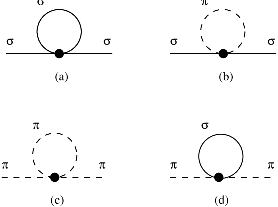
FIG. 1.: One-loop self-energy diagrams for $\sigma$, (a) and (b), and for pions, (c) and (d). Solid line is the free sigma meson propagator and the dashed line is the free pion propagator.

This observation suggests[7] that a partial sum of the infinite series of the loop expansion may be made by imposing the self-consistency condition on the one-loop result replacing the propagators $D_{\sigma/\pi}(k)$ for the intermal lines of the one-loop Feynmann diagrams by the Hartree propagator of the form

$$G_{\beta,\sigma/\pi}^{\rm H}(k)=[k^{2}+M_{\sigma/\pi}^{2}]^{-1}.$$ (61)

We define our “Hartree approximation” by imposing self-consistency conditions for the mass parameters $M_{\sigma/\pi}$ introduced in this propagator: masses

$$M_{\sigma}^{2} = m^{2}+\frac{1}{2}\lambda{\bar{\phi}}^{2}+\Pi_{\beta,\sigma}^{\rm H}(M_{\sigma},M_{\pi}),$$ (62)

$$M_{\pi}^{2} = m^{2}+\frac{1}{6}\lambda{\bar{\phi}}^{2}+\Pi_{\beta,\pi}^{\rm H}(M_{\sigma},M_{\pi})$$ (63)

where two self-energy terms are given by

$$\Pi_{\beta,\sigma}^{\rm H}(M_{\sigma},M_{\pi})=\Pi_{\beta,\pi}^{\rm H}(M_{\sigma},M_{\pi})=\lambda\left[\Phi_{\beta}(M_{\sigma}^{2})+\Phi_{\beta}(M_{\pi}^{2})\right]$$ (64)

with

$$\Phi_{\beta}(M^{2})\equiv\int_{\beta,B}d^{4}k\frac{1}{k^{2}+M^{2}}$$ (65)

where the subscript $B$ is just to remind that the sum is taken over the boson Matsubara frequency. These are the generalization of the Dolan-Jackiw “gap equations” for multi-component fields in the presence of non-vanishing condensate ${\bar{\sigma}}_{\beta}=0$. This approximation is called “modified Hartree approximation” by Baym and Grinstein. Successive substitutions of the right hand sides of the equations into the arguments of the self-energy terms generate an infinite series of “superdaisy diagrams”.

FIG. 2.: Schwinger-Dyson equations in the self-consistent Hartree approximation for thermal sigma meson propagator (a) and for thermal pion propagator (b).

We note that the direct substitution of the internal propagators in the one-loop self-energy for the $\sigma$ field would generate an extra term for the $\sigma$ self-energy $\Pi_{\beta,\sigma}^{\rm H}$,

$$\Delta\Pi_{\beta,\pi}(k:M_{\sigma},M_{\pi})=-\lambda^{2}{\bar{\sigma}}^{2}\left[\Phi_{\beta}^{\prime}(k:M_{\sigma}^{2})+\frac{1}{3}\Phi_{\beta}^{\prime}(k:M_{\pi}^{2})\right]$$ (66)

where

$$\Phi_{\beta}^{\prime}(k:M^{2})\equiv\int_{B}d^{4}k^{\prime}\frac{1}{(k^{\prime 2}+M^{2})((k^{\prime}+k)^{2}+M^{2})}.$$ (67)

We have excluded this term since it has non-trivial $k$ dependence (or “dispersion”) and therefore invalidates our simple ansatz (61) for the Hartree propagator.

FIG. 3.: The diagrams omitted in our approximation.

Our prescription for the self-consistent Hartree approximation is not complete yet since we have not specified the condition for determining the condensate amplitude ${\bar{\sigma}}$ which appears in the self-consistency condition for $\Pi_{\beta,\sigma}^{\rm 1-loop}$. Our guiding principle here is the Goldstone theorem. We replace the one-loop stationary condition for the $\sigma$ field by

$$\left[m^{2}+\frac{1}{6}\lambda{\bar{\sigma}}^{2}+\Pi_{\beta,\pi}^{\rm H}(M_{\sigma},M_{\beta})\right]{\bar{\sigma}}=\epsilon.$$ (68)

This equation, together with (63), implies

$$M_{\pi}^{2}{\bar{\sigma}}=\epsilon$$ (69)

so that it guarantees that the pion becomes massless Goldstone mode in the limit of $\epsilon\to 0$.

C Renormalization

The self-energy terms in one-loop approximation and in self-consistent Hartree approximation contain (quadratic) divergences which all originate from the divergent integral of $\Phi_{\beta}(M)$. These divergence must be removed carefully by the renormalization procedure due to the nonlinear structure of the equations. It turns out, however, that such non-perturbative renormalization is possible only when there is no symmetry breaking ${\bar{\sigma}}=0$ as we shall see below.

We first isolate the divergence in the self-energy terms by performing the Matsubara frequency sum using the formula (42): We find

$$\Phi_{\beta}(M)=\int\frac{d^{3}k}{(2\pi)^{3}}\frac{1}{2\varepsilon_{\bf k}}+{\widetilde{\Phi}}_{\beta}(M)$$ (70)

where

$${\widetilde{\Phi}}_{\beta}(M)=\int\frac{d^{3}k}{(2\pi)^{3}}\frac{1}{\varepsilon_{\bf k}}f_{\rm B}(\varepsilon_{\bf k}).$$ (71)

All divergences in the self-energy terms arise from the phase space integral of the first temperature independent term. The phase space integral of ${\widetilde{\Phi}}_{\beta}(M)$ converges due to the ultraviolet cut-off by the distribution function $f_{\rm B}(ek)$ and this term vanishes at zero temperature. To regularize the divergent integral we introduce the ultraviolet momentum cut-off $\Lambda$ in the phase space integral:

$$\int_{\Lambda}\frac{d^{3}k}{(2\pi)^{3}}\frac{1}{2\varepsilon_{\bf k}}=I_{1}(\Lambda)-M^{2}I_{2}(\Lambda,\mu)+\frac{M^{2}}{16\pi^{2}}\ln\frac{M^{2}}{\mu^{2}}+{\cal O}(\Lambda^{-1})$$ (72)

where

$$I_{1}(\Lambda) \equiv \frac{\Lambda^{2}}{8\pi^{2}},$$ (73)

$$I_{2}(\Lambda,\mu) \equiv \frac{1}{16\pi^{2}}\left[\ln(4\Lambda^{2}/\mu^{2})-1\right]$$ (74)

and $\mu$ is an arbitrary constant which plays the role of a renormalization scale.

We seek the renormalization conditions for the bare parameters $(m,\lambda)$ so that the resultant equations are written only in terms of the renormalized parameters $(m_{R},\lambda_{R})$ and contain only finite terms. For this purpose it is convenient to rewrite the equations (62) and (63) in a more symmetric form. We first add the two equations:

$$M_{\sigma}^{2}+M_{\pi}^{2} = 2m^{2}+\frac{2}{3}\lambda{\bar{\sigma}}^{2}+2\lambda\left[\Phi_{\beta}(M_{\sigma})+\Phi_{\beta}(M_{\pi})\right]$$ (75)

$$= 2m^{2}+4\lambda I_{1}(\Lambda)+\frac{2}{3}\lambda{\bar{\sigma}}^{2}-2\lambda I_{2}(\Lambda,\mu)(M_{\sigma}^{2}+M_{\pi}^{2})$$ (77)

$$\quad+2\lambda\left[\frac{M_{\sigma}^{2}}{16\pi^{2}}\ln\frac{M_{\sigma}^{2}}{\mu^{2}}+\frac{M_{\pi}^{2}}{16\pi^{2}}\ln\frac{M_{\pi}^{2}}{\mu^{2}}\right]+2\lambda\left[{\widetilde{\Phi}}_{\beta}(M_{\sigma})+{\widetilde{\Phi}}_{\beta}(M_{\pi})\right]$$

where we have used (72) in deriving the second line. This equation may be rewritten as

$$M_{\sigma}^{2}+M_{\pi}^{2}=-2m_{R}^{2}+\frac{2}{3}\lambda_{R}{\bar{\sigma}}^{2}+2\lambda_{R}\left[\frac{M_{\sigma}^{2}}{16\pi^{2}}\ln\frac{M_{\sigma}^{2}}{\mu^{2}}+\frac{M_{\pi}^{2}}{16\pi^{2}}\ln\frac{M_{\pi}^{2}}{\mu^{2}}+{\widetilde{\Phi}}_{\beta}(M_{\sigma})+{\widetilde{\Phi}}_{\beta}(M_{\pi})\right]$$ (78)

by imposing the following renormalization conditions[26]:

$$-\frac{m_{R}^{2}}{\lambda_{R}} = \frac{m^{2}}{\lambda}+2I_{1}(\Lambda),$$ (79)

$$\frac{1}{\lambda_{R}} = \frac{1}{\lambda}+2I_{2}(\Lambda,\mu).$$ (80)

On the other hand, however, the subtraction of (63) from (62) gives another relation

$$M_{\sigma}^{2}-M_{\pi}^{2}=\frac{1}{3}\lambda{\bar{\sigma}}^{2}$$ (81)

which contains the bare coupling $\lambda$. In the limit of $\Lambda\to\infty$, the bare coupling goes $\lambda\to 0_{-}$ for any finite $\lambda_{R}$, hence we find

$$M_{\sigma}=M_{\pi}$$ (82)

and in this case the renormalized self-consistency condition (78) becomes simply

$$M^{2}=-m_{R}^{2}+\frac{1}{3}\lambda_{R}{\bar{\sigma}}^{2}+2\lambda_{R}\left[\frac{M^{2}}{16\pi^{2}}\ln\frac{M^{2}}{\mu^{2}}+{\widetilde{\Phi}}_{\beta}(M)\right]$$ (83)

for $M=M_{\sigma}=M_{\pi}$. Unfortunately, this renormalization scheme is possible only when the symmetry is not broken ${\bar{\sigma}}=0$ and $\epsilon=0$ and does not apply for the broken-symmetry phase.

Similar difficulty was noted in [10] for the finite temperature self-consistent approximation similar to ours.

Having seen the difficulty in finding the decent renormalization conditions for our self-consistency conditions, we take an phenomenological approach to the problem: we replace the divergent integral $\Phi_{\beta}(M^{2})$ by its finite temperature-dependent piece ${\widetilde{\Phi}}_{\beta}(M^{2})$ simply discarding the divergent integral associated with the “vacuum loops”. We therefore impose

$$M_{\sigma}^{2} = m^{2}+\frac{1}{2}\lambda{\bar{\phi}}^{2}+\lambda\left[{\widetilde{\Phi}}_{\beta}(M_{\sigma}^{2})+{\widetilde{\Phi}}_{\beta}(M_{\pi}^{2})\right],$$ (84)

$$M_{\pi}^{2} = m^{2}+\frac{1}{6}\lambda{\bar{\phi}}^{2}+\lambda\left[{\widetilde{\Phi}}_{\beta}(M_{\sigma}^{2})+{\widetilde{\Phi}}_{\beta}(M_{\pi}^{2})\right]$$ (85)

for the temperature-dependent effective masses and

$$\left[m^{2}+\frac{1}{6}\lambda{\bar{\phi}}^{2}+\lambda\left({\widetilde{\Phi}}_{\beta}(M_{\sigma}^{2})+{\widetilde{\Phi}}_{\beta}(M_{\pi}^{2})\right)\right]{\bar{\sigma}}=\epsilon$$ (86)

for the condition to determine the amplitude of the condensate.

The physical rationale for this procedure is the observation that each term in the self-energy term, e. g.

$$\lambda{\widetilde{\Phi}}_{\beta}(M^{2})=\lambda\int\frac{d^{3}k}{(2\pi)^{3}}\frac{1}{2\varepsilon_{\bf k}(M)}f_{\rm B}(\varepsilon_{\bf k}(M))$$ (87)

is just due to the forward scattering of the meson by other mesons of effective mass $M$ present in the system. Since the $\sigma$ model should be considered as an effective theory of the underlying microscopy theory of the strong interaction, namely QCD, it would be physically sensible to only take into account the effect of physical excitations in the system as these equations actually do. This approximation also corresponds to neglecting the “many-body” interactions among the thermally excited mesons due to the vacuum loops.

IV Numerical analysis of the gap equations

In this section we present numerical solutions of the gap equations derived in the previous section. It will be shown first that in the exact chiral limit the solutions exhibit hysteresis behavior characteristic of first order phase transition. We will show, however, that the introduction of the finite symmetry breaking term washes away this hysteresis for any choices of model parameters in accordance with the physical conditions.

In constructing numerical solutions of the gap equations (84), (85) and (86), we first note that from (84) and (85) the effective sigma mass is related to the effective pion mass by

$$M_{\sigma}^{2}=M_{\pi}^{2}+\frac{1}{3}\lambda{{\bar{\sigma}}}^{2}$$ (88)

while (85) and (86) imply that the effective pion mass is related to the strength of the explicit symmetry breaking term in the Lagrangian density by

$$M_{\pi}^{2}{\bar{\sigma}}=\epsilon.$$ (89)

What remains to be done is to solve one of the self-consistency condition, say for the effective sigma mass,

$$M_{\sigma}^{2}=m^{2}+\frac{1}{2}\lambda{\bar{\phi}}^{2}+\lambda\left[{\widetilde{\Phi}}_{\beta}(M_{\sigma}^{2})+{\widetilde{\Phi}}_{\beta}(M_{\pi}^{2})\right],$$ (90)

by inserting (88) and (89).

Although the physical value of $\epsilon$ is actually given in terms of the physical pion mass and the pion decay constant by the zero temperature relation ($\epsilon=m_{\pi}^{2}f_{\pi}$), we consider $\epsilon$ as an external variable and examine how the solutions of the gap equations depend on the strength of $\epsilon$.

A Exact chiral limit ($\epsilon=0$):

We first examine the special case when $\epsilon=0$. In this limiting case the chiral symmetry is the exact symmetry of the Lagrangian and according to the Goldstone theorem the pion becomes massless in the low temperature phase where the symmetry is spontaniously broken. Our approximation scheme in fact guarantees this condition by (89). At zero temperature, the above relations (88) and (90) imply

$$M_{\sigma}^{2}(T=0) \equiv m_{0}^{2}=-2m^{2},$$ (91)

$${\bar{\sigma}}^{2}(T=0) \equiv \phi_{0}^{2}=-6m^{2}/\lambda.$$ (92)

In the symmetry broken phase where ${\bar{\sigma}}\neq 0$, $M_{\pi}=0$ and $M_{\sigma}^{2}=\frac{1}{3}\lambda{\bar{\sigma}}^{2}$, the self-consistency condition for the effective sigma meson mass becomes

$${\tilde{M}}_{\sigma}^{2}={\tilde{m}}^{2}+\frac{3}{2}{\tilde{M}}_{\sigma}^{2}+\frac{\lambda}{2\pi^{2}}\left[I^{(2)}_{-}({\tilde{M}}_{\sigma})+I^{(2)}_{-}(0)\right]$$ (93)

where we have introduced dimensionless variable ${\tilde{M}}_{\sigma}\equiv M_{\sigma}\beta$, ${\tilde{m}}=m\beta$ and the dimensionless function $I^{(2)}(\mu)$ is defined by

$$I_{\pm}^{(2)}(\mu)\equiv\int_{0}^{\infty}\frac{x^{2}dx}{\sqrt{x^{2}+\mu^{2}}}\frac{1}{e^{\sqrt{x^{2}+\mu^{2}}}\pm 1}$$ (94)

The high temperature expansion of $I_{\pm}^{(2)}(\mu)$ appropriate for small value of $\mu$ is given in the Appendix B. On the other hand, in the high temperature symmetric phase, where ${\tilde{\sigma}}=0$ and $M_{\sigma}=M_{\pi}$, the gap equations become degenerate to

$${\tilde{M}}_{\sigma}^{2}={\tilde{m}}^{2}+2\lambda\frac{1}{2\pi^{2}}I^{(2)}_{-}({\tilde{M}}_{\sigma})$$ (95)

Using $I_{\pm}^{(2)}(0)=\pi^{2}/6$ the above two conditions are further simplified to

$$\frac{6}{\pi^{2}}I^{(2)}_{-}({\tilde{M}}_{\sigma})=\frac{12}{\lambda}\left[-{\tilde{m}}^{2}-\frac{1}{2}{\tilde{M}}_{\sigma}^{2}\right]-1$$ (96)

for the low temperature phase, and

$$\frac{6}{\pi^{2}}I^{(2)}_{-}({\tilde{M}}_{\sigma})=\frac{6}{\lambda}\left[-{\tilde{m}}^{2}+{\tilde{M}}_{\sigma}^{2}\right]$$ (97)

for the high temperature symmetric phase.

It is instructive to examine the solutions of the above equations graphically. In Fig. 4 we plot the function

$$f(x^{2})=\frac{6}{\pi^{2}}I^{(2)}_{-}(x),$$ (98)

which appear on the left hand side of the above two equations, by the solid line; the right hand sides of (96) and (97) are plotted by dashed curves. The intersection of two curves determines the solutions of the scaled gap equation, (96) or (97), for the scaled sigma mass square ${\tilde{M}}_{\sigma}^{2}$. We note that $f(z)$ is a concave, monotonically decreasing function of $z={\tilde{M}}_{\sigma}^{2}$ normalized as $f(0)=1$, while the right hand sides of (96) and (97) are both linear in $z$. Since the value of $-m^{2}$ is fixed by the amplitude of vacuum condensate at $-m^{2}=1/6\lambda\phi_{0}^{2}(>0)$, the $y$-intercepts of the dashed curves ($-12{\tilde{m}}^{2}/\lambda-1$ for the low temperature phase; $-6{\tilde{m}}^{2}/\lambda$ for the high temperature phase) both move upward as the temperature is lowered, while the solid curve remains unchanged.

FIG. 4.: Graphical construction of the solutions of the gap equations (96) and (97): the solid curve depicts the left hand side of the equations and two dashed lines marked by LT and HT are for the right hand side of (96) and (97), respectively, both as a function of ${{\tilde{M}}_{\sigma}}^{2}$. Crossing points of the solid curve and the dashed line give the solution of the corresponding gap equation.

In the high temperature phase, two curves cross when $-6{\tilde{m}}^{2}/\lambda>1$. The condition $-6{\tilde{m}}^{2}/\lambda=1$ determines the “critical” temperature

$$T_{0}=\phi_{0}$$ (99)

below which the real solution of (97) does not exist. Note that $T_{0}$ does not depend on the strength of the interaction $\lambda$. When one approaches to $T_{0}$ from high temperature side, the effective sigma mass decreases continuously and vanishes at $T=T_{0}$. On the other hand, at low temperatures below $T_{0}$, where $-6{\tilde{m}}^{2}/\lambda>1$, the dashed curve for the low temperature phase intersects with the solid one at one point giving a unique solution to the original gap equations. As the temperature increases, the effective sigma mass again decreases. However, it does not vanish at $T_{0}$ in this case. Instead, as the temperature increases slightly above $T_{0}$, there appears another crossing point at small ${\tilde{M}}_{\sigma}^{2}$ due to the concave shape of the function $I^{(2)}_{-}(\mu)$ as plotted against $\mu^{2}$. As the temperature is further increased, the two crossing points approach toward each other and they eventually annihilate at certain temperature $T_{1}(>T_{0})$ when the dashed line becomes tangent to the solid curve.

We show in Fig. 5 the temperature dependence of the effective sigma mass and the amplitude of the sigma condensate, normalized by their zero temperature values given by (91) and (92) respectively. This plot is made by solving (96) and (97) respectively for $-{\tilde{m}}^{2}$ and making parametric plot of the temperature ($\propto 1/\sqrt{-{\tilde{m}}^{2}}$) vs the scaled sigma mass ($\propto{\tilde{M}}_{\sigma}/\sqrt{-{\tilde{m}}^{2}})$. The scale of the temperature in this plot is set by the value of $T_{0}$ which is equivalent to the amplitude of the vacuum condensate by (99). The system exhibits a typical hysteresis behavior of first order phase transition in the exact chiral limit. We note that this hysteresis appears always irrespective to the value of $\lambda$ since the slope of the function $f(z)$ diverges at $z=0$. The magnitude of $T_{1}$ depends on $\lambda$ explicitly, however. For larger $\lambda$, the slope of the dashed lines in Fig. 4 (b) becomes less steeper, thus $T_{1}$ is larger. Since $T_{0}$ is independent of $\lambda$, this implies that the region of the hysteresis is larger for stronger coupling. We next examine how this behavior is modified when $\epsilon$ is finite.

FIG. 5.: Temperature dependence of the solutions of the gap equations in the chiral limit ($\epsilon=0$) for the scaled sigma mass ($\mu_{\sigma}=M_{\sigma}/m_{0}$) and the scaled sigma condensate ($\chi={\bar{\sigma}}/\phi_{0}$) as a function of $t=T/T_{0}$. In the high temperature phase, the effective pion mass becomes degenerate with the effective sigma mass while it vanishes in the low temperature symmetry broken phase. The scale of the temperature is set by $T_{0}=\phi_{0}$.

B For $\epsilon\neq 0$:

As we have noted earlier, $\epsilon$ plays the role of externally applied magnetic field in the case of magnetic phase transition, therefore we expect that the transition will get smoother for non-vanishing $\epsilon$ .

For our numerical analysis with non-vanishing $\epsilon$, it is more convenient to use the following dimensionless variables:

$$\mu_{\sigma} \equiv M_{\sigma}/m_{0},$$ (100)

$$\mu_{\pi} \equiv M_{\pi}/m_{0},$$ (101)

$$\chi \equiv {\bar{\sigma}}/\phi_{0},$$ (102)

$$t \equiv T/T_{0}=T/\phi_{0},$$ (103)

$${{\tilde{\epsilon}}} \equiv \epsilon/(m_{0}^{2}\phi_{0}),$$ (104)

where $m_{0}$ and $\phi_{0}$ are the sigma mass and the sigma condensate at zero temperature in the limit $\epsilon=0$ as determined by (91) and (92), respectively. The equations (88), (89) and (90) then reduce to

$$\mu_{\sigma}^{2} = \mu_{\pi}^{2}+\chi^{2},$$ (105)

$$\mu_{\pi}^{2}\chi = {{\tilde{\epsilon}}},$$ (106)

$$2\mu_{\sigma}^{2} = -1+3\chi^{2}+\frac{3}{\pi^{2}}t^{2}\left[I^{(2)}_{-}(\sqrt{\lambda/3}\mu_{\sigma}/t)+I^{(2)}_{-}(\sqrt{\lambda/3}\mu_{\pi}/t)\right],$$ (107)

respectively. Note that in this form the $\lambda$ dependence of the gap equation is absorbed into the $\lambda$ dependence of the argument of the dimensionless function $I^{(2)}_{-}$. The solutions of these coupled nonlinear equations depends on two dimensionless parameters, $\lambda$ and ${\tilde{\epsilon}}$. In the limit ${{\tilde{\epsilon}}}\to 0$ they coincide with the previous results.

We show in Fig. 6 the ${\tilde{\epsilon}}$-dependence of the scaled order parameter $\chi$ plotted as a function of the scaled temperature $t$. It is seen that for small values of ${\tilde{\epsilon}}$ the solutions exhibit hysteresis behavior (the back-bending shape of $\chi$). As ${\tilde{\epsilon}}$ increases, however, the curve stretches out gradually and for a large value of ${\tilde{\epsilon}}$, $\chi$ becomes a monotonically decreasing function of temperature. From an inspection of the equations (105), (106) and (107), we can see that the effect of ${\tilde{\epsilon}}$ is expected to become significant when $\chi^{2}\sim\mu_{\pi}^{2}={\tilde{\epsilon}}/\chi$ in (105) or $\sqrt{\lambda/3}\mu_{\pi}/t\sim 1$ for the argument of the second $I^{(2)}_{-}$ in (107); the former condition gives ${\tilde{\epsilon}}\sim\chi^{3}$ and the latter ${\tilde{\epsilon}}\sim 3t^{2}\chi/\lambda$ for the conditions that a significant modification is caused by ${\tilde{\epsilon}}$. This explains why for a relatively small value of ${\tilde{\epsilon}}$, say ${\tilde{\epsilon}}=0.001$, we see in the plot that a considerable modification appears at small $\chi$, $\chi<0.1$, and that for larger $\lambda$ the effect is more significant. We found that the critical value of ${\tilde{\epsilon}}$ for the disappearance of the trace of hysteresis is ${\tilde{\epsilon}}_{c}=0.002$ for $\lambda=100$.

FIG. 6.: Temperature dependence of the scaled order parameter $\chi=\sigma/\sigma_{0}$. The curves are labeled by the value of ${\tilde{\epsilon}}$. Two figures correspond to two different choices of the coupling strength $\lambda$.

The physical value of ${\tilde{\epsilon}}$ may be determined by adjusting the values of our model parameters ($\lambda$, $-m^{2}$ and $\epsilon$) so that they reproduce the physical pion mass ($m_{\pi}=140$MeV), and the pion decay constant $f_{\pi}=93$MeV and the sigma mass $m_{\sigma}$ in the vacuum. In the linear sigma model $f_{\pi}$ is identified as the amplitude of the vacuum condensate: $\sigma_{0}=f_{\pi}$. Then (88) and (90) give constraints:

$$m_{\sigma}^{2}=m_{\pi}^{2}+\frac{1}{3}\lambda f_{\pi}^{2}=m^{2}+\frac{1}{2}\lambda f_{\pi}^{2},$$ (108)

which implies

$$\lambda=3(m_{\sigma}^{2}-m_{\pi}^{2})/f_{\pi}^{2}$$ (109)

and

$$-m^{2}=(m_{\sigma}^{2}-3m_{\pi}^{2})/2.$$ (110)

We note that since $-m^{2}>0$ these two relations give a constraint $\lambda>6m_{\pi}^{2}/f_{\pi}^{2}=13.6$ on the allowed values for $\lambda$. When we vary $\lambda$ from 50 to 500, $m_{\sigma}$ varies from 400 MeV to 1200 MeV constrained by these relations. The corresponding values of ${\tilde{\epsilon}}=\epsilon/m_{0}^{2}\phi_{0}$ are determined by using $m_{0}^{2}=-2m^{2}$ and $\phi_{0}=f_{\pi}/\chi_{0}$ where $\chi_{0}$ is the solution of the scaled gap equation at zero temperature. Some representative results are tabulated in Table I. For large coupling $\lambda$, the sigma mass increases as $m_{\sigma}\sim m_{0}\sim\sqrt{\lambda/3}f_{\pi}$ and the relative strength of the symmetry breaking term decreases as ${{\tilde{\epsilon}}}=(m_{\pi}/m_{0})^{2}(f_{\pi}/\phi_{0})\sim 3\lambda^{-1}(m_{\pi}/f_{\pi})^{2}$. We show in Fig. 7 the results for the temperature dependence of the mass parameter for two different choices of the coupling strength $\lambda$.

FIG. 7.: Temperature dependence of the effective sigma mass ($M_{\sigma}$) and the effective pion mass ($M_{\pi}$) for $\epsilon$ ($=m_{\pi}^{2}f_{\pi}$). Two figures correspond to two different choices of the coupling strength $\lambda$.

An interesting question is whether the hysterisis can survive for a sufficiently large value of $\lambda$ since ${\tilde{\epsilon}}$ decreases for large $\lambda$. This is not the case, however, since the critical value of the ${\tilde{\epsilon}}$ also decreases for small $\lambda$. One can see this point noting that the argument of the second $I^{(2)}_{-}$ in (107) becomes independent of $\lambda$ at large $\lambda$: $\sqrt{\lambda/3}\mu_{\pi}/t\sim(m_{\pi}/f_{\pi})/\sqrt{\chi}t$ as $\lambda\rightarrow\infty$. For any value of $\lambda$ the introduction of the symmetry breaking term $\epsilon=m_{\pi}^{2}f_{\pi}$ with physical value for $m_{\pi}$ and $f_{\pi}$ washes away the hysteresis behavior in the solution of the gap equatioon.

V Summary

In this paper we have studied the chiral phase transition at finite temperature using the meson sector of the linear sigma model. We formulated a self-consistent approximation scheme starting from the one-loop effective potential by imposing self-consistency conditions on the effective meson mass equation, keeping the meson self-energy independent of meson momentum. The resultant equations are just the Dolan-Jackiw gap equations for multi-component fields in the presence of non-vanishing meson condensate. In this approximation, the meson mass parameter in the thermal (imaginary time) meson propagator may be identified by analytic continuation as the mass of the real mesonic excitations introduced in the system in equilibrium although in more general cases such simple identification is not possible. This non-perturbative approximation scheme has, however, a difficulty in choosing proper renormalization conditions to eliminate the divergent loop integrals. We therefore adopted a phenomenological approach which just ignores the divergent vacuum loops. This procedure is technically equivalent to introduce a zero momentum cut-off in the vacuum loop integral.

We showed that the solutions of the resultant gap equations does not reproduce usual second order phase transition. We found, instead, that they exhibit hysteresis behavior characteristic of the first order transition in the chiral limit. It is shown that this “premature transition” is caused by the long range fluctuation of the mesons fields whose effective masses become small in the transition region. We are however not able to calculate the transition temperature from the gap equations alone; to do so we need the information of the effective potential associated with the approximation we employed in this work. Such calculation may be performed by the method of the composite operator effective potential developped by Cornwall, Jackiw, and Tomboulis[28]. We have made a preliminary investigation in this direction[29]. The result will be reported elsewhere.

Inclusion of the symmetry breaking term generally tends to smooth sharp phase transition, but in general, the first order transition may survive if the symmetry breaking scale is small enough. We found, however, that this is not the case at least in our calculation: the physical pion mass, together with the PCAC relation for the axial current, gives a very strong constraint on the choice of the parameters of our model and the hysteresis behavior is smoothed out irrespective of the coupling strength. We found that smooth chiral transition takes place at $T=150\sim 200$MeV in our model, consistent with recent results from the state-of-art lattice QCD calculations at finite temperature[13]. An advantage of the present approach based on the effective degrees of freedom, expressing crucial aspects of the symmetry behavior of the system, is that it is more tractable for investigating more difficult problem of the dynamics of the chiral transition in high energy nuclear collisions where we expect non-equilibrium aspects may play essential role [18, 19, 20]. We also plan to investigate this problem in the future.

A Inclusion of Baryon

The original $\sigma$ model Lagrangian contains the baryon (nucleon) fields coupled to meson fields by Yukawa coupling. At low temperatures ($T<<m_{N}$), we may expect the contribution of the thermal baryon-antibaryon excitations is negligible. This may not be so however near the transition temperature since the baryon mass becomes smaller due to the reduction of the $\sigma$ condensate which dynamically generates the baryon mass. For example, in the lowest order of the Yukawa coupling $g$,

$$m_{N}=g{\bar{\sigma}},$$ (A1)

(see Fig. baryon-self). We show in this appendix that the inclusion of the baryon fluction in this approximation leads to the results very similar to the Hartree approximation without baryons. However, we show also that it is not a consistent approximation for the meson propagators.

FIG. 8.: The lowest order baryon self-energy diagram

Inclusion of the baryonic excitations in the computation of the effective potential may be performed in the line similar to mesonic excitations (Sect. 2) with one modification that the functional integral over the Grassmann variables, which represent “classical fermion field”, leads to the change of the sign and the removal of the factor $1/2$ in the one-loop contribution:

$$V_{1,\rm baryon}^{\beta}({\bar{\phi}}_{a})=\int d^{4}k\ln\det G_{N}(k)$$ (A2)

where

$$G_{N}(k)=\frac{1}{\not k+M_{N}}$$ (A3)

is the thermal Green’s function for baryons with $\not k\equiv i\omega_{n}\gamma_{0}+\gamma_{i}k_{i}$ and the sum is taken over the fermion Matsubara frequency $\omega_{n}=(2n+1)\pi\beta^{-1}$ which arises from the anti-periodic boundary conditions for fermionic fields in the path integral. The nucleon mass matrix is given here by

$$M_{N}=g({\bar{\sigma}}+i\gamma_{5}{\bf{\bar{\pi}}}_{i}{\bar{\tau}}_{i})$$ (A4)

for non-vanishing ${\bar{\phi}}_{a}=({\bar{\sigma}},{\bf\bar{\pi}})$. Inserting (A3) into (A2) and performing the determinant over Lorentz and isospin indices we find

$$V_{1,\rm baryon}^{\beta}({\bar{\phi}}_{a})=-2\cdot 2\int d^{4}k\ln[k^{2}+g^{2}{\bar{\phi}}^{2}]$$ (A5)

where $k^{2}=\omega_{n}^{2}+{\bf k}^{2}$. In this result, one factor 2 has arisen from determinant in the Lorentz indices and may be attributed to the spin degrees of freedom, while another factor 2 is due to the isospin degrees of freedom. Note that fermionic loop contribution is larger than that of bosonic loop by another factor 2 due to the distinction of particle and anti-particle in case of fermion. In the presence of non-vanishing pion field $g^{2}{\bar{\phi}}^{2}$ plays the role of the square of the effective nucleon mass, as expected simply from the symmetry consideration.

Adding this term to the effective potential gives rise to new terms in the stationary conditions for the meson fields and the meson mass equations. We could modify our “Hartree approximation” by inserting the following term to the meson self-energy to the right hand side of (62) and (63) :

$$\Pi_{\beta,\sigma}^{N}(m_{N})=\Pi_{\beta,\pi}^{N}(m_{N})=-8g^{2}\Psi_{\beta}(m_{N}^{2})$$ (A6)

with

$$\Psi_{\beta}(M)\equiv\int_{F}d^{4}k\frac{1}{k^{2}+M^{2}}$$ (A7)

where the factor $8=2\cdot 2\cdot 2$ in (A6) accounts for the particle-antiparticle, spin, and isospin degeneracy and the subscript $F$ in (A7) indicates that the sum is taken over the fermionic Matsubara frequency.

This result resembles remarkablly the ones we have obtained for the meson loop contribution to the meson self-energies (64). Inclusion of the baryon loop contribution to the meson self-energy is not a consistent procedure, however, in view of the procedure we have adopted to drop the diagrams in Fig. 3, since both diagrams generate non-trivial momentum dependence or dispersion in the self-energy of mesons and thus again invalidates our ansatz (61) for the meson propagators.

FIG. 9.: Baryon loop diagrams which contribute to the self-energy of sigma (a) and pion (b)

B High temperature expansion of one-loop integrals

Phase space integral in one-loop diagrams contain definite integrals of the following form:

$$I_{\pm}^{(n)}(\mu)\equiv\int_{0}^{\infty}\frac{x^{n}dx}{\sqrt{x^{2}+\mu^{2}}}\frac{1}{e^{\sqrt{x^{2}+\mu^{2}}}\pm 1}.$$ (B1)

For example, the boson (fermion) loop contributions to the meson self-energies is

$${\widetilde{\Phi}}_{\beta}(M)=\int\frac{d^{3}k}{(2\pi)^{3}}\frac{1}{E_{k}}\frac{1}{e^{\beta E_{k}}\pm 1}=\beta^{-2}\frac{1}{2\pi^{2}}I_{\pm}^{(2)}(M\beta),$$ (B2)

while the pressure of ideal gas of boson (fermion) with mass $M$ is

$$P(\beta;M)\equiv\pm\beta^{-1}\int\frac{d^{3}k}{(2\pi)^{3}}\ln\left[1\pm e^{-\beta\sqrt{k^{2}+M^{2}}}\right]=\beta^{-4}\frac{1}{6\pi^{2}}I_{\pm}^{(4)}(M\beta),$$ (B3)

where $+(-)$ sign is for fermion (boson).

The functions $I^{(n)}_{\pm}(\mu)$ satisfy the following recursion relations:

$$\frac{d}{d\mu^{2}}I^{(n)}_{\pm}(\mu)=-\frac{n-1}{2}I^{(n-2)}_{\pm}(\mu)$$ (B4)

and have the following limits for $\mu\to 0$:

$$I^{(n)}_{-}(0) = \Gamma(n)\zeta(n),$$ (B5)

$$I^{(n)}_{+}(0) = (1-2^{1-n})\Gamma(n)\zeta(n),$$ (B6)

where $\Gamma(x)$ is the gamma function and $\zeta(x)=\sum_{m=1}^{\infty}1/m^{x}$ is the Riemann $\zeta$ function.

We wish to evaluate the integral $I^{(n)}_{\pm}(\mu)$ for the small nonvanishing value of $\mu=M\beta$, corresponding to high temperatures ($T>>M$), however, the power series expansion of $I^{(n)}_{\pm}(\mu)$ would break down at $\mu^{n}$ since the gamma function $\Gamma(x)$ is singular at negative integer values of $x$. These singularities originate from the infrared (small $x$) part of the integral $I^{(n)}_{\pm}$. In the case of boson it is enhanced due to the additional singular behavior of the distribution function of massless boson at small $x$: $1/(e^{x}-1)\sim 1/x$.

Series expansion of $I_{\pm}^{(n)}(\mu)$ was derived by Dolan and Jackiw in [27] for even integer value of $n$. Here we quote some of their useful results:

$$I^{(0)}_{-} = \frac{\pi}{2\mu}+\frac{1}{2}\ln\frac{\mu}{4\pi}+\frac{1}{2}\gamma+\frac{1}{2}\sum_{n=1}^{\infty}\frac{1}{n}\left[\left(1+\frac{\mu^{2}}{4\pi^{2}n^{2}}\right)^{-1/2}-1\right]$$ (B7)

$$= \frac{\pi}{2\mu}+\frac{1}{2}\ln\frac{\mu}{4\pi}+\frac{1}{2}\gamma+\frac{\zeta(3)}{16\pi}\mu^{2}-\frac{3\zeta(5)}{64\pi^{2}}\mu^{4}+{\cal O}(\mu^{6}),$$ (B8)

$$I^{(0)}_{+} = -\frac{1}{2}\ln\frac{\mu}{\pi}-\frac{1}{2}\gamma+\frac{1}{2}\sum_{n=1}^{\infty}\frac{1}{n}\left[\left(1+\frac{\mu^{2}}{4\pi^{2}n^{2}}\right)^{-1/2}-1\right]$$ (B9)

$$= -\frac{1}{2}\ln\frac{\mu}{\pi}-\frac{1}{2}\gamma+\frac{\zeta(3)}{16\pi}\mu^{2}-\frac{3\zeta(5)}{64\pi^{2}}\mu^{4}+{\cal O}(\mu^{6})$$ (B10)

where $\gamma=0.57721\cdots$ is Euler’s number and the numerical values of the $\zeta$ function at relevant points are $\zeta(2)=\pi^{2}/6$, $\zeta(3)=1.2020\cdots$, $\zeta(4)=\pi^{4}/90$, $\zeta(5)=1.0369\cdots$, and so on. The series expansion of $I^{(2)}_{\pm}(\mu)$ and $I^{(4)}_{\pm}(\mu)$ can be obtained from (B8) and (B10) by integrating the differential equation (B4) with the boundary conditions (B5) or (B6):

$$I^{(2)}_{\pm}(\mu) = I^{(2)}_{\pm}(0)-\frac{1}{2}\int_{0}^{\mu^{2}}d\mu^{\prime 2}I^{(0)}_{\pm}(\mu^{\prime}),$$ (B11)

$$I^{(4)}_{\pm}(\mu) = I^{(4)}_{\pm}(0)-\frac{3}{2}\int_{0}^{\mu^{2}}d\mu^{\prime 2}I^{(2)}_{\pm}(\mu^{\prime}).$$ (B12)

The result is

$$I^{(2)}_{-}(\mu) = \frac{\pi^{2}}{6}-\frac{\pi}{2}\mu-\frac{1}{4}\mu^{2}\ln\frac{\mu}{4\pi}+\left(\frac{1}{8}-\frac{1}{4}\gamma\right)\mu^{2}-\frac{\zeta(3)}{32\pi}\mu^{4}+{\cal O}(\mu^{6}),$$ (B13)

$$I^{(4)}_{-}(\mu) = \frac{\pi^{4}}{15}-\frac{\pi^{2}}{4}\mu^{2}+\frac{\pi}{2}\mu^{3}+\frac{3}{16}\mu^{4}\ln\frac{\mu}{4\pi}-\frac{3}{8}\left(\frac{3}{4}-\gamma\right)\mu^{4}+{\cal O}(\mu^{6}),$$ (B14)

for boson and

$$I^{(2)}_{+}(\mu) = \frac{\pi^{2}}{12}+\frac{1}{4}\mu^{2}\ln\frac{\mu}{\pi}+\frac{1}{4}\left(-\frac{1}{2}+\gamma\right)\mu^{2}-\frac{\zeta(3)}{32\pi}\mu^{4}+{\cal O}(\mu^{6}),$$ (B15)

$$I^{(4)}_{+}(\mu) = \frac{7\pi^{4}}{120}-\frac{\pi^{2}}{8}\mu^{2}-\frac{3}{16}\mu^{4}\ln\frac{\mu}{\pi}-\frac{3}{32}\left(\frac{3}{2}-2\gamma\right)\mu^{4}+{\cal O}(\mu^{6}),$$ (B16)

for fermion.

$\lambda$	$m_{\sigma}$ (MeV)	${{\tilde{\epsilon}}}=\epsilon/(m_{0}^{2}\phi_{0})$
50	404	0.219
100	555	0.0846
200	772	0.0378
500	1208	0.0142
1000	1703	0.0069

TABLE I.: $\lambda$ dependence of the sigma meson mass at zero temperature and the scaled symmetry breaking parameter

REFERENCES

- [1]
- [2] S. Weinberg, in Chiral Dynamics:Theory and Experiments eds. A. Bernstein and B. Holstein (Springer, 1995) p. 3; H. Leutwyler, ibid, p. 14.
- [3] Y. Nambu, Phys. Rev. Lett. 4, 380 (1960); Y. Nambu and G. Jona-Lasinio, Phys. Rev. 122, 345 (1961).
- [4] J. Goldstone, Nuovo Cimento 19, 154 (1961); J. Goldstone, A. Salam, and S. Weinberg, Phys. Rev. 127, 965 (1962).
- [5] For example, see H. E. Stanley, Introduction to Phase Transitions and Critical Phenomena, Oxford University Press, Inc. (New York, 1971).
- [6] D. A. Kirzhnits and A. D. Linde, Phys. Lett. 42 B, 471 (1972); Ann. Phys. 101, 195 (1976).
- [7] L. Dolan and R. Jackiw, Phys. Rev. D 9, 3320 (1974).
- [8] S. Weinberg, Phys. Rev. D 9, 3357 (1974).
- [9] T. D. Lee and G. C. Wick, Phys. Rev. D 9, 2291 (1974).
- [10] G. Baym and G. Grinstein, Phys. Rev. D 15, 2897 (1977).
- [11] M. Gell-Mann, and M. Levy, Nuovo Cimento 16, 705 (1960).
- [12] B. Lee, Chiral Dynamics (Gordon and Breach, 1970).
- [13] For review of recent works, see: A. Ukawa, Lattice 89, Nucl. Phys. B (Proc. Suppl.) 17 (1990) 118; S. Gottlieb, Lattice 90, Nucl. Phys. B (Proc. Suppl.) 20 (1991) 118; F. Karsch, Lattice 93, Nucl. Phys. B (Proc. Suppl.) 34 (1994) 63. K. Kanaya, to appear in the proceedings of Lattice 95.
- [14] T. Hatsuda and T. Kunihiro, Phy. Rev. Lett. 55, 158 (1985); Prog. Theor. Phy. 74, 765 (1985).
- [15] S. Weinberg, Phys. Rev. Lett. 18, 188 (1967); Physics 96A, 327 (1979).
- [16] J. Gasser and H. Leutwyler, Phys. Lett. B 184, 83 (1987); Nucl. Phys. B 307, 763 (1988); ibid 321, 387 (1989).
- [17] J.D. Bjorken, Int. J. Mod. Phys. A 7 (1987) 4189; J. D. Bjorken, K. Kowalski and C. Taylor, SLAC preprint, SLAC-PUB-6109 (1993)
- [18] K. Rajagopal and F. Wilczek, Nucl. Phys. B404 (1993) 577; S. Gavin, A. Gocksch, and R.D. Pisarski, Phys. Rev. Lett. 72 2143 (1994); S. Gavin, and B. Müller, Phys. Lett. B329, 486 (1994); M. Asakawa, Z. Huang, X. -N. Wang, Phys. Rev. Lett. 74, 3126 (1995); J. Randrup, Phys. Rev. Lett. 77, 1226 (1996).
- [19] D. Boyanovsky, H. J. de Vega, and R. Holman, Phys. Rev. D 51, 734 (1995).
- [20] F. Cooper, Y. Kluger, E. Mottola, and J. P. Paz; Phys. Rev. D 51, 2377 (1995).
- [21] We follow the notation in C. Itzykson and J.-B. Zuber, Quantum Field Theory (McGraw-Hill, New York, 1980).
- [22] B. D. Serot, and J. D. Walecka, Advances in Nuclear Physics 16, eds. J. W. Negele and E. Vogt, Plenum Press, New York (1986).
- [23] A. Fetter, and J. D. Walecka, Quantum Theory of Many-Particle Systems (McGraw-Hill, New York, 1971).
- [24] J. Kapusta, Finite-Temperature Field Theory (Cambridge University Press, Cambridge, 1989).
- [25] R. Jackiw, Phys. Rev. D 9, 1686 (1974).
- [26] S. Coleman, R. Jackiw, and H. D. Politzer, Phys. Rev. D 10, 2491 (1974); M. Kobayashi, and T. Kugo, Prog. Theor. Phys. 54, 1537 (1975); see also, A. Kerman and D. Vautherin, Ann. Phys. 192, 408 (1989).
- [27] Ref. [7] appendix C.
- [28] J. M. Cornwall, R. Jackiw, and E. Tomboulis, Phys. Rev. D 10, 2428 (1974); G. Amelino-Camelia and S.-Y. Pi, Phys. Rev. D 47, 2356 (1993).
- [29] H.-S. Roh, J. Korean Phys. Soc. (Proc. Suppl.) 29, S372 (1996).