NIKHEF 96-028
VUTH 96-07
nucl-th/9611040 Prospects for spin physics
in semi-inclusive processes

Abstract

I discuss inclusive and semi-inclusive lepton-hadron scattering emphasizing the importance of polarization in order to study various single or double spin asymmetries and the importance of particle identification and angular resolution in the dectection of final state particles to study azimuthal asymmetries. The observables obtained in this way enable a detailed study of quark and gluon correlations in hadrons.

1 Introduction

The reason that spin has become a hot topic in deep inelastic scattering (DIS) is not only due to the progress in beam and target polarization enabling new experiments, but it is as important that there exists a clear view of what one actually measures. In particular this is the case for sum rules that measure a well-determined local matrix element of quark and gluon field operators. For instance the integral $\int dx\ g_{1}^{N}(x)$ measures an axial current matrix element. For $\int dx\ (g_{1}^{p}-g_{1}^{n})(x)$ this is even an combination that gives up to a factor the nucleon axial charge, a number that can also be obtained from neutron $\beta$-decay, a relation known as the Bjorken sumrule.

The topic of this talk will be the relation of DIS observables to matrix elements of quark and gluon operators. In order to establish such a relation one needs to consider hard scattering processes in which a large scale $Q$ – in lepton-hadron scattering the four momentum transfer squared $-q^{2}\equiv Q^{2}$ – is present. The leading part of the cross section is related to matrix elements that have a simple interpretation as quark and gluon distributions. Subleading parts in an expansion in $1/Q$ involve matrix elements of combinations of quarks and gluon fields, i.e. quark-gluon correlation functions. These are known as higher twist contributions. A particular feature that I want to emphasize is the role of transverse momenta of quarks. To probe them one needs for example semi-inclusive processes such as 1-particle inclusive leptoproduction. The momentum of the produced hadron defines a direction orthogonal to the fast direction defined by the (spacelike) virtual photon and the target hadron. A similar role can be played by the spin vector if the target hadron is transversely polarized. Anyway as will become evident polarization plays an important role in this talk.

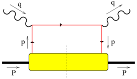
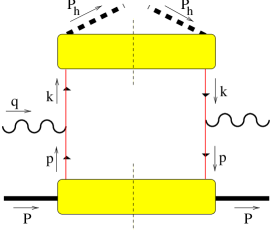
Figure 1: The simplest (parton-level) diagrams representing the squared amplitude in lepton hadron inclusive scattering (left) en semi-inclusive scattering (right).

One of the aims of deep inelastic leptoproduction is the study of the quark and gluon structure of the hadronic target using the known framework of Quantum chromodynamics (QCD). Thus, as a theorist the aim is to calculate the hadronic tensor $W_{\mu\nu}$ by making a diagrammatic expansion. Already at the simplest level (Fig. 1) a problem is encountered, namely there are hadrons involved for which QCD does not provide rules. Thus, soft parts are identified that allow inclusion of hadrons in the field theoretical framework. Furthermore it will turn out that for $Q^{2}\rightarrow\infty$ only a limited number of diagrams is needed.

2 Soft parts

The soft parts can be written down in terms of quark and gluon fields as illustrated below. They are characterized by the fact that the momenta are soft with respect to each other. We have for the distribution part [1, 2]

$$\mbox{with}\ \ p^{2}\sim p\cdot P\sim P^{2}=M^{2}\ll Q^{2}$$

represented by

$$\Phi_{ij}(p,P,S)=\frac{1}{(2\pi)^{4}}\int d^{4}x\;e^{ip\cdot x}\;\langle P,S|\overline{\psi}_{j}(0)\psi_{i}(x)|P,S\rangle,$$ (1)

and the fragmentation part [3]

$$\mbox{with}\ \ k^{2}\sim k\cdot P_{h}\sim P_{h}^{2}=M_{h}^{2}\ll Q^{2}$$

represented by

$$\Delta_{ij}(k,P_{h},S_{h})$$

$$\qquad=\sum_{X}\frac{1}{(2\pi)^{4}}\int d^{4}x\;e^{ik\cdot x}\langle 0|\psi_{i}(x)|P_{h},S_{h};X\rangle\langle P_{h},S_{h};X|\overline{\psi}_{j}(0)|0\rangle.$$ (2)

In order to find out which information in the soft parts $\Phi$ and $\Delta$ is important in a hard process one needs to realize that the hard scale $Q$ leads in a natural way to the use of lightlike vectors $n_{+}$ and $n_{-}$ satisfying $n_{+}^{2}=n_{-}^{2}=0$ and $n_{+}\cdot n_{-}$ = 1. For inclusive deep inelastic scattering

$$\left.\begin{array}[]{l}q^{2}=-Q^{2}\\ P^{2}=M^{2}\\ 2\,P\cdot q=\frac{Q^{2}}{x_{{}_{B}}}\end{array}\right\}\longleftrightarrow\left\{\begin{array}[]{l}P=\frac{x_{{}_{B}}M^{2}}{Q\sqrt{2}}\,n_{-}+\frac{Q}{x_{{}_{B}}\sqrt{2}}\,n_{+}\\ \mbox{}\\ q=\frac{Q}{\sqrt{2}}\,n_{-}-\frac{Q}{\sqrt{2}}\,n_{+}\end{array}\right.$$

Comparing the power of $Q$ with which the momenta in the soft and hard part appear one immediately is led to the fact that $\int dp^{-}\,\Phi(p,P,S)$ is the relevant quantity to investigate,

part	’components’
	$-$	+
HARD	$\sim Q$	$\sim Q$
$H\rightarrow q$	$\sim 1/Q$	$\sim Q$	$\rightarrow\int dp^{-}\ldots$

For 1-particle inclusive scattering one parametrizes the momenta as

$$\left.\begin{array}[]{l}q^{2}=-Q^{2}\\ P^{2}=M^{2}\\ P_{h}^{2}=M_{h}^{2}\\ 2\,P\cdot q=\frac{Q^{2}}{x_{{}_{B}}}\\ 2\,P_{h}\cdot q=-z_{h}\,Q^{2}\end{array}\right\}\longleftrightarrow\left\{\begin{array}[]{l}P_{h}=\frac{z_{h}\,Q}{\sqrt{2}}\,n_{-}+\frac{M_{h}^{2}}{z_{h}\,Q\sqrt{2}}\,n_{+}\\ \mbox{}\\ q=\frac{Q}{\sqrt{2}}\,n_{-}-\frac{Q}{\sqrt{2}}\,n_{+}+q_{T}\\ \mbox{}\\ P=\frac{x_{{}_{B}}M^{2}}{Q\sqrt{2}}\,n_{-}+\frac{Q}{x_{{}_{B}}\sqrt{2}}\,n_{+}\end{array}\right.$$

and it follows that one needs besides the quantity $\int dp^{-}\,\Phi(p,P,S)$ the equivalent for the fragmentation part, $\int dk^{+}\,\Delta(k,P_{h},S_{h})$.

part	’components’
	$-$	+
$q\rightarrow h$	$\sim Q$	$\sim 1/Q$	$\rightarrow\int dk^{+}\ldots$
HARD	$\sim Q$	$\sim Q$
$H\rightarrow q$	$\sim 1/Q$	$\sim Q$	$\rightarrow\int dp^{-}\ldots$

3 Analysis of soft parts: distribution and fragmentation functions

Hermiticity, parity and time reversal invariance (T) constrain the quantity $\Phi(p,P,S)$. It must be of the form [4, 5]

$$\Phi(k,P,S) = M\,A_{1}+A_{2}\,\kern 1.99997ptP\kern-5.59998pt\raisebox{1.29167pt}{/}+A_{3}\kern 1.99997ptk\kern-4.49997pt/+i\,A_{4}\,\frac{[\kern 1.99997ptP\kern-5.59998pt\raisebox{1.29167pt}{/},\kern 1.99997ptk\kern-4.49997pt/]}{2M}+i\,A_{5}\,(k\cdot S)\gamma_{5}$$ (3)

$$+M\,A_{6}\,\kern 1.99997ptS\kern-5.59998pt\raisebox{1.29167pt}{/}\gamma_{5}+A_{7}\,\frac{k\cdot S}{M}\,\kern 1.99997ptP\kern-5.59998pt\raisebox{1.29167pt}{/}\gamma_{5}+A_{8}\,\frac{k\cdot S}{M}\kern 1.99997ptk\kern-4.49997pt/\gamma_{5}+A_{9}\,\frac{[\kern 1.99997ptP\kern-5.59998pt\raisebox{1.29167pt}{/},\kern 1.99997ptS\kern-5.59998pt\raisebox{1.29167pt}{/}]\gamma_{5}}{2}$$

$$+A_{10}\,\frac{[\kern 1.99997ptk\kern-4.49997pt/,\kern 1.99997ptS\kern-5.59998pt\raisebox{1.29167pt}{/}]\gamma_{5}}{2}+A_{11}\,\frac{k\cdot S}{M}\,\frac{[\kern 1.99997ptP\kern-5.59998pt\raisebox{1.29167pt}{/},\kern 1.99997ptk\kern-4.49997pt/]\gamma_{5}}{2M}+A_{12}\,\frac{\epsilon_{\mu\nu\rho\sigma}\gamma^{\mu}P^{\nu}k^{\rho}S^{\sigma}}{M},$$

with real $A_{i}$ = $A_{i}(k^{2},k\cdot P)$ and if T applies $A_{4}=A_{11}=A_{12}=0$.

This imposes constraints on the functions allowed in the Dirac projections $\Phi^{[\Gamma]}$ defined as

$$\Phi^{[\Gamma]}(x,\mbox{\boldmath$p$}_{T}) = \int dp^{-}\,\frac{Tr[\Phi\Gamma]}{2}$$ (4)

$$= \left.\int\frac{d\xi^{-}d^{2}\mbox{\boldmath$\xi$}_{T}}{2\,(2\pi)^{3}}\ e^{ip\cdot\xi}\,\langle P,S|\overline{\psi}(0)\Gamma\psi(\xi)|P,S\rangle\right|_{\xi^{+}=0},$$

which is a lightfront ($\xi^{+}$ = 0) correlation function. The relevant projections in $\Phi$ that are important in leading order in $1/Q$ in hard processes are

$$\Phi^{[\gamma^{+}]}(x,{\mbox{\boldmath$p$}}_{{}_{T}}) = f_{1}(x,{\mbox{\boldmath$p$}}_{{}_{T}}^{2})$$ (5)

$$\Phi^{[\gamma^{+}\gamma_{5}]}(x,{\mbox{\boldmath$p$}}_{{}_{T}}) = \lambda\,g_{1L}(x,{\mbox{\boldmath$p$}}_{{}_{T}}^{2})+\frac{({\mbox{\boldmath$p$}}_{{}_{T}}\cdot{\mbox{\boldmath$S$}}_{{}_{T}})}{M}\,g_{1T}(x,{\mbox{\boldmath$p$}}_{{}_{T}}^{2})$$ (6)

$$\Phi^{[i\sigma^{i+}\gamma_{5}]}(x,{\mbox{\boldmath$p$}}_{{}_{T}}) = S_{T}^{i}\,h_{1}(x,{\mbox{\boldmath$p$}}_{{}_{T}}^{2})+\frac{\lambda\,p_{T}^{i}}{M}\,h_{1L}^{\perp}(x,{\mbox{\boldmath$p$}}_{{}_{T}}^{2})$$ (7)

$${}-\frac{\left(p_{T}^{i}p_{T}^{j}+\frac{1}{2}{\mbox{\boldmath$p$}}_{{}_{T}}^{2}g_{T}^{ij}\right)S_{Tj}}{M^{2}}\,h_{1T}^{\perp}(x,{\mbox{\boldmath$p$}}_{{}_{T}}^{2})$$

Here $x=p^{+}/P^{+}$ and the (lightcone) helicity $\lambda$ and transverse spin $S_{T}$ of the target hadron are defined as

$$\left.\begin{array}[]{l}P^{2}=M^{2}\\ S^{2}=-1\\ P\cdot S=0\end{array}\right\} \longleftrightarrow \left\{\begin{array}[]{l}P=\frac{M^{2}}{2P^{+}}\,n_{-}+P^{+}\,n_{+}\\ S=-\lambda\frac{M}{2P^{+}}\,n_{-}+\lambda\frac{P^{+}}{M}\,n_{+}+S_{T}\end{array}\right.$$

$$\quad(\lambda^{2}+\mbox{\boldmath$S$}_{T}^{2}=1)$$

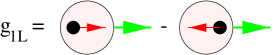
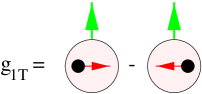
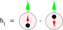
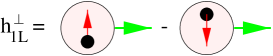
Figure 2: The interpretation of the leading twist functions appearing in the Dirac projections of the soft part $\Phi$.

All functions appearing above can be interpreted as momentum space densities, as illustrated in Fig. 2. The first, denoted $f_{\ldots}^{\ldots}$ (in naming we follow ref. [6]) involve the operator structure

$$\Phi^{[\gamma^{+}]}\propto\overline{\psi}\gamma^{+}\psi=\psi_{+}^{\dagger}\psi_{+},$$ (9)

where $\psi_{+}=P_{+}\psi$ with $P_{+}=\gamma^{-}\gamma^{+}/2$. This operator projects on the socalled good component of the Dirac field, which can be considered as a free dynamical degree of freedom in front form quantization. It is precisely in this sense that partons measured in hard processes are free. The functions $g_{\ldots}^{\ldots}$ and $h_{\ldots}^{\ldots}$ appearing above are differences of densities for opposite quark polarizations. In the case of $g_{\ldots}^{\ldots}$ it is the difference of densities for quark chirality states $\psi_{R/L}=P_{R/L}\psi$ with $P_{R/L}=(1\pm\gamma_{5})/2$,

$$\Phi^{[\gamma^{+}\gamma_{5}]}\propto\overline{\psi}\gamma^{+}\gamma_{5}\psi=\psi_{+R}^{\dagger}\psi_{+R}-\psi_{+L}^{\dagger}\psi_{+L},$$ (10)

while in the case of $h_{\ldots}^{\ldots}$ it is the difference of densities for quark transverse spin states $\psi_{\uparrow/\downarrow}=P_{\uparrow/\downarrow}\psi$ with $P_{\uparrow/\downarrow}=(1\pm\gamma^{1}\gamma_{5})/2$,

$$\Phi^{[\sigma^{1+}\gamma_{5}]}\propto\overline{\psi}\sigma^{1+}\gamma_{5}\psi=\psi_{+\uparrow}^{\dagger}\psi_{+\uparrow}-\psi_{+\downarrow}^{\dagger}\psi_{+\downarrow}.$$ (11)

The projectors $P_{R/L}$ and $P_{\uparrow/\downarrow}$ commute with $P_{+}$.

Theorists often are more happy with lightcone correlation functions, because they can employ and isolate lightcone singularities and proof factorization theorems. These appear in the ${\mbox{\boldmath$p$}}_{{}_{T}}$-integrated quantities

$$\Phi^{[\Gamma]}(x) = \int dp^{-}\,d^{2}\mbox{\boldmath$p$}_{T}\,\frac{Tr[\Phi\Gamma]}{2}$$ (13)

$$= \left.\int\frac{d\xi^{-}}{4\pi}\ e^{ip\cdot\xi}\,\langle P,S|\overline{\psi}(0)\Gamma\psi(\xi)|P,S\rangle\right|_{\begin{array}[]{l}\xi^{+}=|\mbox{\boldmath$\xi$}_{T}|=0\end{array}}$$

The above constraints on $\xi$ imply $\xi^{2}=0$. The ${\mbox{\boldmath$p$}}_{{}_{T}}$-averaged results which are relevant for inclusive lepton-hadron or ${\mbox{\boldmath$q$}}_{{}_{T}}$-averaged Drell-Yan are

$$\Phi^{[\gamma^{+}]}(x)=f_{1}(x),$$ (14)

$$\Phi^{[\gamma^{+}\gamma_{5}]}(x)=\lambda\,g_{1}(x),$$ (15)

$$\Phi^{[i\sigma^{i+}\gamma_{5}]}(x)=S_{T}^{i}\,h_{1}(x).$$ (16)

It is useful to remark here that flavor indices have been omitted, i.e. one has $f_{1}^{u}$, $f_{1}^{d}$, etc. At this point it may also be good to mention other notations used frequently such as $f_{1}^{u}(x)=u(x)$, $g_{1}^{u}(x)=\Delta u(x)$, $h_{1}^{u}(x)=\Delta_{T}u(x)$, etc. We note that some of the ${\mbox{\boldmath$p$}}_{{}_{T}}$-dependent functions have vanished. They do appear, however, in ${\mbox{\boldmath$p$}}_{{}_{T}}/M$-weighted results relevant for azimuthal asymmetries in 1-particle inclusive $\ell H$ or DY,

$$\Phi_{\partial}^{\alpha[\Gamma]}(x) \equiv \int dp^{-}\,d^{2}\mbox{\boldmath$p$}_{T}\ p_{T}^{\alpha}\frac{Tr[\Phi\Gamma]}{2}$$ (18)

$$= \left.\int\frac{d\xi^{-}}{4\pi}\ e^{ip\cdot\xi}\,\langle P,S|\overline{\psi}(0)\Gamma\,i\partial^{\alpha}\psi(\xi)|P,ngle\right|_{\begin{array}[]{l}\xi^{+}=|\mbox{\boldmath$\xi$}_{T}|=0\end{array}}$$

Two ${\mbox{\boldmath$p$}}_{{}_{T}}/M$-weighted results (relevant for asymmetries in $\ell H$ or DY) are

$$\frac{1}{M}\,\Phi_{\partial}^{\alpha[\gamma^{+}\gamma_{5}]}(x)=S_{T}^{\alpha}\,g_{1T}^{(1)}(x),$$ (19)

$$\frac{1}{M}\,\Phi_{\partial}^{\alpha[i\sigma^{i+}\gamma_{5}]}(x)=-g_{T}^{\alpha i}\,\lambda\,h_{1L}^{\perp(1)}(x),$$ (20)

where the functions with superscript $(1)$ denote ${\mbox{\boldmath$p$}}_{{}_{T}}^{2}$-moments,

$$g_{1T}^{(1)}(x)\equiv\int d^{2}{\mbox{\boldmath$p$}}_{{}_{T}}\,\frac{{\mbox{\boldmath$p$}}_{{}_{T}}^{2}}{2M^{2}}\,g_{1T}(x,{\mbox{\boldmath$p$}}_{{}_{T}}).$$ (21)

The analysis of the soft part $\Phi$ can be extended to other Dirac projections. Limiting ourselves to ${\mbox{\boldmath$p$}}_{{}_{T}}$-averaged functions one finds the following possibilities,

$$\Phi^{[1]}(x)=\frac{M}{P^{+}}\,e(x),$$ (22)

$$\Phi^{[\gamma^{i}\gamma_{5}]}(x)=\frac{M\,S_{T}^{i}}{P^{+}}\,g_{T}(x),$$ (23)

$$\Phi^{[i\sigma^{+-}\gamma_{5}]}(x)=\frac{M}{P^{+}}\,\lambda\,h_{L}(x).$$ (24)

Lorentz covariance requires for these projections on the right hand side a factor $M/P^{+}$, which as can be seen from the earlier given parametrization of momenta produces a suppression factor $M/Q$ and thus these functions appear at subleading order in cross sections. Furthermore, these functions can not be written in the form of densities or difference of densities. However, interesting relations between these functions and the above ${\mbox{\boldmath$p$}}_{{}_{T}}/M$-weighted functions can be obtained [7, 8] using the most general amplitude analysis for $\Phi$, constrained by hermiticity, parity and time reversal invariance,

$$g_{2}\ =\ g_{T}-g_{1}\ =\ \frac{d}{dx}\,g_{1T}^{(1)},$$ (25)

$$h_{2}\ =\ 2(h_{L}-h_{1})\ =\ -2\,\frac{d}{dx}\,h_{1L}^{\perp(1)}.$$ (26)

Just as for the distribution functions one can perform an analysis of the soft part describing the quark fragmentation [8]. The Dirac projections in this case are

$$\Delta^{[\Gamma]}(z,{\mbox{\boldmath$k$}}_{{}_{T}}) = \int dk^{+}\,\frac{Tr[\Delta\Gamma]}{4z}$$ (27)

$$= \left.\sum_{X}\int\frac{d\xi^{+}d^{2}\mbox{\boldmath$\xi$}_{T}}{4z\,(2\pi)^{3}}\,e^{ik\cdot\xi}\,Tr\langle 0|\psi(x)|P_{h},X\rangle\langle P_{h},X|\overline{\psi}(0)\Gamma|0\rangle\right|_{\xi^{-}=0}.$$

The relevant projections in $\Delta$ that appear in leading order in $1/Q$ in hard processes are for the case of no final state polarization,

$$\Delta^{[\gamma^{-}]}(z,{\mbox{\boldmath$k$}}_{{}_{T}})=D_{1}(z,-z{\mbox{\boldmath$k$}}_{{}_{T}}),$$ (28)

$$\Delta^{[i\sigma^{i-}\gamma_{5}]}(z,{\mbox{\boldmath$k$}}_{{}_{T}})=\frac{\epsilon_{T}^{ij}k_{Tj}}{M_{h}}\,H_{1}^{\perp}(z,-z{\mbox{\boldmath$k$}}_{{}_{T}}).\qquad\mbox{[T-odd]}$$ (29)

The arguments of the fragmentation functions $D_{1}$ and $H_{1}^{\perp}$ are chosen to be $z$ = $P_{h}^{-}/k^{-}$ and $\mbox{\boldmath$P$}_{h\perp}$ = $-z{\mbox{\boldmath$k$}}_{{}_{T}}$. The first is the (lightcone) momentum fraction of the produced hadron, the second is the transverse momentum of the produced hadron with respect to the quark. The fragmentation function $D_{1}$ is the equivalent of the distribution function $f_{1}$. It can be interpreted as the probability of finding a hadron $h$ in a quark. Adding quark flavor index ($a$) and kind of produced hadron the distribution functions are normalized as $\sum_{h}\int dz\,d^{2}P_{h\perp}\,zD_{1}(z,P_{h\perp})$ = 1. Noteworthy is the appearance of the function $H_{1}^{\perp}$, interpretable as the different production probability of unpolarized hadrons from a transversely polarized quark (see Fig. 3). This functions has no equivalent in the distribution functions and is allowed because of the non-applicability of time reversal invariance because of the appearance of out-states $|P_{h},X\rangle$ in $\Delta$, rather than the plane wave states in $\Phi$.

Figure 3: The interpretation of the leading twist functions appearing in the Dirac projections of the soft part $\Delta$ for unpolarized hadrons.

After ${\mbox{\boldmath$k$}}_{{}_{T}}$-averaging one is left with the function

$$\Delta^{[\gamma^{-}]}(z)=D_{1}(z),$$ (30)

while the ${\mbox{\boldmath$k$}}_{{}_{T}}/M$-weighted result is

$$\frac{1}{M}\,\Delta_{\partial}^{\alpha[i\sigma^{i-}\gamma_{5}]}(z)=-\epsilon_{T}^{\alpha i}\,H_{1}^{\perp(1)}(z),$$ (31)

with

$$H_{1}^{\perp(1)}(z)\equiv z^{2}\int d^{2}{\mbox{\boldmath$k$}}_{{}_{T}}\,\frac{{\mbox{\boldmath$k$}}_{{}_{T}}^{2}}{2M_{h}^{2}}\,H_{1}(z,-z{\mbox{\boldmath$k$}}_{{}_{T}}).$$ (32)

At subleading order in hard processes one finds after ${\mbox{\boldmath$k$}}_{{}_{T}}$-averaging the following fragmentation functions

$$\Delta^{[1]}(z)=\frac{M_{h}}{P_{h}^{-}}\,E(z),$$ (33)

$$\Delta^{[i\sigma^{ij}\gamma_{5}]}(z)=\frac{M_{h}\,\epsilon_{T}^{ij}}{P_{h}^{-}}\,H(z).$$ (34)

Again a relation with the ${\mbox{\boldmath$k$}}_{{}_{T}}/M$-weighted functions exist, namely

$$\frac{H(z)}{z}\ =\ z^{2}\,\frac{d}{dz}\,\left[\frac{H_{1}^{\perp(1)}}{z}\right].$$ (35)

We summarize the analysis of the soft part with a table of distribution and fragmentation functions for unpolarized (U), longitudinally polarized (L) and transversely polarized (T) targets, distinguishing leading (twist two) and subleading (twist three, appearing at order $1/Q$) functions and furthermore distinguishing the chirality. Chiral even functions are diagonal in the space of chiral quark states, which is the case for Dirac projections $\gamma^{\mu}$ or $\gamma^{\mu}\gamma_{5}$ (thus the functions $f$, $g$, $D$ and $G$); chiral odd functions are nondiagonal in this basis, which is the case for Dirac projections $1$, $i\gamma_{5}$ or $i\sigma^{\mu\nu}\gamma_{5}$ (thus the functions $e$, $h$, $E$ and $H$). The functions printed in boldface survive after integration over transverse momenta.
DISTRIBUTIONS chirality $\Phi^{[\Gamma]}$ even odd U ${\mbox{\boldmath$f$}}_{1}$ twist 2 L ${\mbox{\boldmath$g$}}_{1L}$ $h_{1L}^{\perp}$ T $g_{1T}$ ${\mbox{\boldmath$h$}}_{1}\ \ {h_{1T}^{\perp}}$ U ${f^{\perp}}$ $e$ twist 3 L ${g_{L}^{\perp}}$ ${\mbox{\boldmath$h$}}_{L}$ T ${\mbox{\boldmath$g$}}_{T}\ \ {g_{T}^{\perp}}$ ${h_{T}}\ \ {h_{T}^{\perp}}$ (9 independent functions) FRAGMENTATION chirality $\Delta^{[\Gamma]}$ even odd U ${\mbox{\boldmath$D$}}_{1}$ ${H_{1}^{\perp}}$ twist 2 L ${\mbox{\boldmath$G$}}_{1L}$ ${H_{1L}^{\perp}}$ T ${G_{1T}}\ \ {D_{1T}^{\perp}}$ ${\mbox{\boldmath$H$}}_{1}\ \ {H_{1T}^{\perp}}$ U ${D^{\perp}}$ $E$    $H$ twist 3 L ${G_{L}^{\perp}}\ \ {D_{L}^{\perp}}\ \ {\mbox{\boldmath$E$}}_{L}$ ${\mbox{\boldmath$H$}}_{L}$ T ${\mbox{\boldmath$G$}}_{T}\ \ {G_{T}^{\perp}}\ \ {\mbox{\boldmath$D$}}_{T}\ \ {E_{T}}$ ${H_{T}}\ \ {H_{T}^{\perp}}$ (12 independent functions)
Note that the number of independent functions is determined by the number of amplitudes $A_{i}$ in the amplitude analysis, i.e. 9 and 12 for distribution and fragmentation functions respectively.

4 Cross sections for lepton-hadron scattering

Having completed the analysis of the soft parts, the next step is to find out how one obtains the information on the various correlation functions from experiments. We will limit ourselves here to lepton-hadron scattering via one-photon exchange. The relevant kinematic (scaling) variables are given in the figure.
$\displaystyle\ell H\longrightarrow\ell^{\prime}hX$ $\displaystyle x_{{}_{B}}=\frac{Q^{2}}{2P\cdot q}$ $\displaystyle y=\frac{P\cdot q}{P\cdot k}$ $\displaystyle z_{h}=\frac{P\cdot P_{h}}{P\cdot q}$
To get the leading order result for semi-inclusive scattering it is sufficient to compute the diagram in Fig. 1 (plus the antiquark analogue) by using QCD and QED Feynman rules in the hard part and the matrix elements $\Phi$ and $\Delta$ for the soft parts, parametrized in terms of distribution and fragmentation functions. The results are:

Cross sections (leading in $1/Q$) $\displaystyle\frac{d\sigma_{OO}}{dx_{{}_{B}}\,dy\,dz_{h}}=\frac{2\pi\alpha^{2}\,s}{Q^{4}}\,\sum_{a,\bar{a}}e_{a}^{2}\left\lgroup 1+(1-y)^{2}\right\rgroup x_{{}_{B}}{f^{a}_{1}}(x_{{}_{B}})\,{D^{a}_{1}}(z_{h})$ (36) $\displaystyle\frac{d\sigma_{LL}}{dx_{{}_{B}}\,dy\,dz_{h}}=\frac{2\pi\alpha^{2}\,s}{Q^{4}}\,{\lambda_{e}\,\lambda}\,\sum_{a,\bar{a}}e_{a}^{2}\ y(2-y)\ x_{{}_{B}}{g^{a}_{1}}(x_{{}_{B}})\,{D^{a}_{1}}(z_{h})$ (37)

One recognizes in these well-known cross sections the characteristic structure of the 1-particle inclusive cross sections, namely the cross section $2\pi\,\alpha^{2}\,s/Q^{4}$ multiplying a kinematic factor (depending on $y$) and a sum over flavors of a product of a distribution function depending on $x_{{}_{B}}$ and a fragmentation function depending on $z_{h}$.

Some general rules on where to find a specific correlation function are the following:

• Depending on the twist $t$ of correlation functions, they appear in cross sections suppressed by a factor $\propto(1/Q)^{t-2}$.

• Cross sections are chirally even. This means e.g. that one finds combinations like $f_{1}\,D_{1}$, ${h_{1}}\,{H_{1}}$ or ${e}\,{H_{1}^{\perp}}$. However, quark mass terms are chirally odd, i.e. one may encounter combinations like $m\,{f_{1}}\,{H_{1}^{\perp}}$.

• The number of spin vectors is even in case of a T-even fragmentation function, i.e. there are only double spin asymmetries, such as ${\lambda_{e}\,\lambda}\,{g_{1}}\,{D_{1}}$, ${\lambda_{e}\,|\mbox{\boldmath$S$}_{T}|}\,{g_{1T}^{(1)}}\,{D_{1}}$ or ${|\mbox{\boldmath$S$}_{T}|\,|\mbox{\boldmath$S$}_{hT}|}\,{h_{1}}\,{H_{1}}$.

• The number of spin vectors is odd in case of a T-odd fragmentation function, i.e. there are only single spin asymmetries, such as ${\lambda_{e}}\,{e}\,{H_{1}^{\perp}}$, ${\lambda}\,{h_{1L}^{\perp(1)}}\,{H_{1}^{\perp}}$ or ${|\mbox{\boldmath$S$}_{hT}|}\,{f_{1}}\,{D_{T}}$.

Two examples of subleading cross sections are [8, 9]

Cross sections subleading in $1/Q$ $\displaystyle\frac{2\pi\,d\sigma_{{OT}}}{dx_{{}_{B}}\,dy\,dz_{h}\,d\phi_{e}}=\frac{2\pi\alpha^{2}\,s}{Q^{4}}\,{|\mbox{\boldmath$S$}_{T}|}\,\sin(\phi_{S})\,2(2-y)\sqrt{1-y}$ $\displaystyle\hskip 113.81102pt\mbox{}\times\sum_{a,\bar{a}}e_{a}^{2}\,\frac{2M}{Q}\,x_{{}_{B}}{h^{a}_{1}}(x_{{}_{B}})\,\frac{{\tilde{H}^{a}}(z_{h})}{z_{h}},$ (38) $\displaystyle\mbox{note:}\ \frac{{\tilde{H}^{a}}(z)}{z}=\frac{H^{a}(z)}{z}+2\,H_{1}^{\perp(1)\,a}(z)=\frac{d}{dz}\left[z\,H_{1}^{\perp(1)\,a}\right],$ $\displaystyle\frac{2\pi\,d\sigma_{{LT}}}{dx_{{}_{B}}\,dy\,dz_{h}\,d\phi_{e}}=\frac{2\pi\alpha^{2}\,s}{Q^{4}}\,{\lambda_{e}|\mbox{\boldmath$S$}_{T}|}\,\cos(\phi_{S})\,2y\sqrt{1-y}$ $\displaystyle\hskip 28.45274pt\mbox{}\times\sum_{a,\bar{a}}e_{a}^{2}\Biggl{\{}\frac{2M}{Q}\,x_{{}_{B}}^{2}{g_{T}^{a}}(x_{{}_{B}})\,{D_{1}^{a}}(z_{h})+\frac{2M_{h}}{Q}\,x_{{}_{B}}{h_{1}^{a}}(x_{{}_{B}})\,\frac{{\tilde{E}^{a}}(z_{h})}{z_{h}}\Biggr{\}},$ (39) $\displaystyle\mbox{note:}\ \frac{{\tilde{E}^{a}}(z)}{z}=\frac{E^{a}(z)}{z}-\frac{m_{a}}{M_{h}}\,D_{1}^{a}(z).$

The tilde functions that appear in the cross sections are in fact precisely the socalled interaction dependent parts of the twist three functions. They would vanish in any naive parton model calculation in which cross sections are obtained by folding e-parton cross sections with parton densities. Considering the relation for $\tilde{E}$ one can state it as $E(z)/z$ = $(m/M_{h})\,D_{1}(z)$ in the absence of quark-quark-gluon correlations. The inclusion of the latter also require diagrams dressed with gluons (see next section).

In 1-particle inclusive processes, one actually becomes sensitive to quark transverse momentum dependent structure functions already for unpolarized targets. Comparing with inclusive scattering one has four structure functions for unpolarized leptons instead of two (longitudinal $W_{L}$ and transverse $W_{T}$). One of the additional (interference) structure functions ($W_{LT}$) has a azimuthal dependence $\propto\cos(\phi_{h})$. This structure function is order $1/Q$ and involves the twist three distribution function $f^{\perp}$ and the fragmentation function $D^{\perp}$, of the latter again only the interaction-dependent part. With polarized leptons (target still unpolarized) a fifth structure function can be measured proportional to $\sin(\phi_{h})$, involving the distribution function $e$ and the time-reversal odd fragmentation function $H_{1}^{\perp}$. Explicitly one has [10]

Azimuthal asymmetries for unpolarized targets (higher twist) $\displaystyle\int d^{2}\mbox{\boldmath$P$}_{h\perp}\,\frac{|\mbox{\boldmath$P$}_{h\perp}|}{M\,z_{h}}\,cos(\phi_{h})\,\frac{d\sigma_{{OO}}}{dx_{{}_{B}}\,dy\,dz_{h}\,d^{2}\mbox{\boldmath$P$}_{h\perp}}=-\frac{2\pi\alpha^{2}\,s}{Q^{4}}\,2(2-y)\sqrt{1-y}$ $\displaystyle\hskip 113.81102pt\mbox{}\times\sum_{a,\bar{a}}e_{a}^{2}\Biggl{\{}\frac{2M}{Q}\,x_{{}_{B}}^{2}{f_{1}^{\perp(1)a}}(x_{{}_{B}})\,{D_{1}^{a}}(z_{h})$ $\displaystyle\hskip 156.49014pt\mbox{}+\frac{2M_{h}}{Q}\,x_{{}_{B}}{f_{1}^{a}}(x_{{}_{B}})\,\frac{{\tilde{D}^{\perp(1)a}}(z_{h})}{z_{h}}\Biggr{\}}$ (40) $\displaystyle\mbox{note:}\ {\tilde{D}^{\perp a}}(z)=D^{\perp a}(z)-zD_{1}^{a}(z),$ $\displaystyle\int d^{2}\mbox{\boldmath$P$}_{h\perp}\,\frac{|\mbox{\boldmath$P$}_{h\perp}|}{M\,z_{h}}\,sin(\phi_{h})\,\frac{d\Delta\sigma_{{LO}}}{dx_{{}_{B}}\,dy\,dz_{h}\,d^{2}\mbox{\boldmath$P$}_{h\perp}}=\frac{2\pi\alpha^{2}\,s}{Q^{4}}\,{\lambda_{e}}\,2y\sqrt{1-y}$ $\displaystyle\hskip 113.81102pt\mbox{}\times\sum_{a,\bar{a}}e_{a}^{2}\,\frac{2M}{Q}\,x_{{}_{B}}^{2}{\tilde{e}^{a}}(x_{{}_{B}})\,{H_{1}^{\perp(1)a}}(z_{h})$ (41) $\displaystyle\mbox{note:}\ {\tilde{e}^{a}}(x)=e^{a}(x)-\frac{m_{a}}{M}\,\frac{f_{1}^{a}(x)}{x}.$

Leading order azimuthal asymmetries also exist. They require polarized targets and give access to the twist two functions $g_{1T}^{(1)}$ and $h_{1L}^{\perp(1)}$. These are particularly intersting in view of the relations with the twist three functions $g_{T}$ and $h_{L}$. One can check this relation and/or use these cross sections as an alternate way to find these functions. One has [11, 12, 13]

Azimuthal asymmetries for polarized targets (leading twist) $\displaystyle\int d^{2}\mbox{\boldmath$P$}_{h\perp}\,\frac{|\mbox{\boldmath$P$}_{h\perp}|}{M\,z_{h}}\,cos(\phi_{h}-\phi_{S})\,\frac{d\sigma_{{LT}}}{dx_{{}_{B}}\,dy\,dz_{h}\,d^{2}\mbox{\boldmath$P$}_{h\perp}}$ $\displaystyle\hskip 56.9055pt=\frac{2\pi\alpha^{2}\,s}{Q^{4}}\,{\lambda_{e}\,|{\mbox{\boldmath$S$}}_{{}_{T}}|}\,y(2-y)\sum_{a,\bar{a}}e_{a}^{2}\,x_{{}_{B}}\,{g_{1T}^{(1)a}}(x_{{}_{B}}){D^{a}_{1}}(z_{h}),$ (42) $\displaystyle\int d^{2}\mbox{\boldmath$P$}_{h\perp}\,\frac{|\mbox{\boldmath$P$}_{h\perp}|^{2}}{MM_{h}\,z_{h}^{2}}\,sin(2\phi_{h})\,\frac{d\Delta\sigma_{{OL}}}{dx_{{}_{B}}\,dy\,dz_{h}\,d^{2}\mbox{\boldmath$P$}_{h\perp}}$ $\displaystyle\hskip 56.9055pt=\frac{2\pi\alpha^{2}\,s}{Q^{4}}\,{\lambda}\,2(1-y)\sum_{a,\bar{a}}e_{a}^{2}\,x_{{}_{B}}\,{h_{1L}^{\perp(1)a}}(x_{{}_{B}}){H_{1}^{\perp(1)a}}(z_{h}),$ (43)
$\displaystyle\int d^{2}\mbox{\boldmath$P$}_{h\perp}\,d\phi_{e}\,\frac{|\mbox{\boldmath$P$}_{h\perp}|}{M_{h}\,z_{h}}\,sin(\phi_{h}+\phi_{S})\,\frac{d\Delta\sigma_{{OT}}}{dx_{{}_{B}}\,dy\,dz_{h}\,d\phi_{e}\,d^{2}\mbox{\boldmath$P$}_{h\perp}}$ $\displaystyle\hskip 56.9055pt=\frac{2\pi\alpha^{2}\,s}{Q^{4}}\,{|{\mbox{\boldmath$S$}}_{{}_{T}}|}\,2(1-y)\sum_{a,\bar{a}}e_{a}^{2}\,x_{{}_{B}}\,{h_{1}^{a}}(x_{{}_{B}}){H_{1}^{\perp(1)a}}(z_{h}).$ (44)

Note that these are leading contributions in the cross section. At subleading order the same asymmetries may have higher harmonics, such as a $\sin(3\phi_{h}-\phi_{S})$ asymmetry appearing in $\Delta\sigma_{OT}$ $\sim$ ${h_{1T}^{\perp(2)}}{H_{1}^{\perp(1)}}$.

I want to end this section with giving an indication of the magnitude of a ${\mbox{\boldmath$k$}}_{{}_{T}}$-dependent distribution functions, in particular look at $g_{1T}^{(1)}(x)$. For this we use the relation of this function with $g_{2}$, namely $g_{1T}^{(1)}(x)$ = $-\int_{x}^{1}dy\,g_{2}(y)$ and the SLAC E143 data on $g_{2}$. The result is shown in Fig. 4 (left panel). Except for the data also the result obtained from the Wandzura-Wilczek part of $g_{2}$, namely $g_{2}^{WW}(x)$ = $-g_{1}(x)+\int_{x}^{1}dy\,(g_{1}(y)/y)$ (omitting quark mass terms). This result is shown in Fig. 4 (left panel) as the solid line [14].

Figure 4: Left panel: the function $g_{1T}^{(1)}$ estimated from the E143 data on $g_{2}$ (datapoints) and from the Wandzura-Wilczek part of $g_{2}$ (solid line); right panel: the resulting asymmetry in $ep\rightarrow e\pi^{+}X$.

The resulting asymmetry in $\sigma_{LT}$ is except for kinematical factors depending on $y$ proportional to the ratio $g_{1T}^{(1)}(x)/f_{1}(x)$. For the case of $\pi^{+}$ production in polarized lepton scattering off a transversely polarized proton, it is dominantly the u-quark that contributes. This ratio is shown in the right panel of Fig. 4.

5 The full calculation and concluding remarks

In the previous section the lowest order results of the calculations of 1-particle inclusive lepton-hadron scattering have been presented. What other effects are important in these cross sections. As emphasized before, QCD is believed to provide a reliable framework to obtain the soft parts. Within this framework we can also indicate some theoretical and experimental caveats.

For this, lets write down the first few diagrams in the full calculation within the field theoretical approach

The first contribution is the parton model result, giving the expressions as derived in the previous section. It is important to realize that its validity requires $P\cdot P_{h}\gg M^{2}$, the current fragmentation region in which there is a sufficiently large rapidity gap between target remnant and produced particles.
The case that $P\cdot P_{h}\sim M^{2}$, the target fragmentation region involves by the definition of soft parts, those soft parts that contain both target and produced hadron (fracture functions) [15]. These parts need a separate theoretical treatment. The use of the results derived previously is limited to the current fragmentation region.
Diagrams containing gluons attached to the soft part (one example shown) need to be considered carefully. They are of two types:
• Longitudinal $A^{+}$ ($A^{-}$) gluons. They do contribute at leading order, but can be absorbed into the definition of the soft parts, creating the link operator that renders the definition of $\Phi$ ($\Delta$) color gauge invariant. • Transverse $A_{T}^{\alpha}$ gluons. They contribute at order $1/Q$. They do not lead to new independent distribution (fragmentation) functions, courtesy of the QCD equations of motion. They ensure electromagnetic gauge invariance of the full calculation at order $1/Q$.
The next corrections that we want to consider are quark and gluon ladders. They give the asymptotic ${\mbox{\boldmath$p$}}_{{}_{T}}$-dependence of the distribution functions, which turns out to be proportional to $\alpha_{s}/{\mbox{\boldmath$p$}}_{{}_{T}}^{2}$.

For the integrated distribution functions, this leads to $\alpha_{s}\log(Q^{2}/\mu^{2})$ contributions. These can be incorporated into a scale dependence of the distribution functions, described with the GLAP equations.
The final QCD corrections which we discuss are process dependent $\alpha_{s}$ corrections, for 1-particle inclusive scattering arising from a diagram as shown here. A characteristic example for inclusive DIS is the longitudinal part, $\displaystyle F_{L}=\frac{F_{2}}{x}-2F_{1}\sim\alpha_{s}(Q^{2})\times\ldots.$

In my talk I have tried to present results that show the prospects of spin physics in semi-inclusive, in particular 1-particle inclusive lepton-hadron scattering. The goal is the study of the quark and gluon structure of hadrons, emphasizing the spin structure and the dependence on quark transverse momenta. The reason why the prospect is promising is the existence of a field theoretical framework that allows a clean study involving well-defined hadronic matrix elements.

This work is part of the scientific program of the foundation for Fundamental Research on Matter (FOM), the Dutch Organization for Scientific Research (NWO) and the TMR program ERB FMRX-CT96-0008.

References

• [1] D.E. Soper, Phys. Rev. D 15 (1977) 1141; Phys. Rev. Lett. 43 (1979) 1847.
• [2] R.L. Jaffe, Nucl. Phys. B 229 (1983) 205.
• [3] J.C. Collins and D.E. Soper, Nucl. Phys. B 194 (1982) 445.
• [4] J.P. Ralston and D.E. Soper, Nucl.Phys. B 152 (1979) 109.
• [5] R.D. Tangerman and P.J. Mulders, Phys. Rev. D 51 (1995) 3357.
• [6] R.L. Jaffe and X. Ji, Nucl. Phys. B 375 (1992) 527.
• [7] A.P. Bukhvostov, E.A. Kuraev and L.N. Lipatov, Sov. Phys. JETP 60 (1984) 22.
• [8] R.D. Tangerman and P.J. Mulders, Nucl. Phys. B 461 (1996) 197.
• [9] R.L. Jaffe and X. Ji, Phys. Rev. Lett. 71 (1993) 2547.
• [10] J. Levelt and P.J. Mulders, Phys. Rev. D 49 (1994) 96; Phys. Lett. B 338 (1994) 357.
• [11] J. Collins, Nucl. Phys. B 396 (1993) 161.
• [12] A. Kotzinian, Nucl. Phys. B 441 (1995) 234.
• [13] R.D. Tangerman and P.J. Mulders, Phys. Lett. B 352 (1995) 129.
• [14] A. Kotzinian and P.J. Mulders, Phys. Rev. D 54 (1996) 1229.
• [15] L. Trentadue and G. Veneziano, Phys. Lett. B 323 (1994) 201.