Resonance contributions to HBT correlation radii

Abstract

We study the effect of resonance decays on intensity interferometry for heavy ion collisions. Collective expansion of the source leads to a dependence of the two-particle correlation function on the pair momentum ${\bf K}$. This opens the possibility to reconstruct the dynamics of the source from the ${\bf K}$-dependence of the measured “HBT radii”. Here we address the question to what extent resonance decays can fake such a flow signal. Within a simple parametrization for the emission function we present a comprehensive analysis of the interplay of flow and resonance decays on the one- and two-particle spectra. We discuss in detail the non-Gaussian features of the correlation function introduced by long-lived resonances and the resulting problems in extracting meaningful HBT radii. We propose to define them in terms of the second order $q$-moments of the correlator $C({\bf q,K})$. We show that this yields a more reliable characterisation of the correlator in terms of its width and the correlation strength $\lambda$ than other commonly used fit procedures. The normalized fourth-order $q$-moments (kurtosis) provide a quantitative measure for the non-Gaussian features of the correlator. At least for the class of models studied here, the kurtosis helps separating effects from expansion flow and resonance decays, and provides the cleanest signal to distinguish between scenarios with and without transverse flow.

I Introduction

The only known way to obtain direct experimental information on the space-time structure of the particle emitting source created in a relativistic nuclear collision is through two-particle intensity interferometry [1, 2]. This information is therefore indispensable for an assessment of theoretical models which try to reconstruct the final state of the collision from the measured single particle spectra and particle multiplicity densities in momentum space. Reliable estimates of the source geometry at particle freeze-out are crucial for an experimental proof that high energy heavy ion collisions can successfully generate large volumes of matter with high energy density. Direct information from two-particle correlations on the expansion dynamics at freeze-out further provides essential constraints for theoretical models which extrapolate back in time towards the initial stages of the collision in order to make statements about a possible transition to deconfined quark matter.

An important insight from recent theoretical research on Hanbury-Brown–Twiss (HBT) interferometry is that for dynamical sources which undergo collective expansion the HBT radius parameters, which characterize the width of the two-particle correlation function, develop a dependence on the pair momentum [3, 4, 5, 6, 7, 8, 9, 10, 11, 12, 13]. The detailed momentum dependence is somewhat model-dependent, and in general it is not simple [11]. Still, it opens the crucial possibility to extract dynamical information on the source from interferometry data. Unfortunately, the most abundant candidates for interferometry studies, charged pions, are strongly contaminated by decay products from unstable resonances some of which only decay long after hadron freeze-out [14, 8]. Such resonance decays were shown to introduce an additional momentum dependence of the HBT radius parameters and of the intercept parameter [8, 15] which complicates the extraction of the expansion flow.

A systematic approach towards extracting the expansion velocity from experimental HBT data thus presupposes a careful analysis of the interplay of flow and resonance decays on the gross features of the two-particle correlation function. This is the aim of the present paper. We will use for our analysis a simple analytical model for the source function, which assumes local thermalization at freeze-out and produces hadronic resonances by thermal excitation. The model incorporates longitudinal and transverse expansion as well as a finite duration of particle emission. The two most important parameters for our considerations, the temperature and transverse expansion velocity at freeze-out, can be varied independently. Our study thus complements published HBT analyses of source functions generated by hydrodynamic simulations where freeze-out is implemented along a sharp hypersurface [8] and which do not allow easily to gain physical intuition by a systematic variation of the model parameters. After freeze-out the resonances are allowed to decay according to an exponential proper time distribution along their trajectories, and the resulting emission functions of daughter particles (pions, kaons, etc.) are added to the direct emission function of particles of the same kind before calculating the correlation function. A discussion of the momentum dependence of resonance decay effects on the 1- and 2-particle spectra requires the correct treatment of the decay phase-space [8, 16, 17] and does not permit the simplifying approximations leading, e.g., to Eq. (1) in Ref. [18].

The paper is organized as follows: In Sec. II we review the extraction of space-time information on the source from Gaussian fits to the correlation function. This calculational scheme is then extended in Sec. III to include resonance decay contributions. The next three sections are devoted to a detailed model study based on this formalism. In Sec. IV we describe the model for the emission function including resonance contributions. Results for the one- and two-particle spectra are presented in Sec. V, and a general discussion of the effects from resonance decays on the shape of the correlation function is given there. In Sec. VI we then discuss in detail the practical difficulties posed by the non-Gaussian features in the correlation function due to long-lived resonances, by comparing different fitting procedures. This leads us in Sec. VII to the alternative method of $q$-moments which provide a clean definition of the HBT radii and intercept parameter even for non-Gaussian correlation functions. These HBT radii show much weaker resonance decay effects than the ones obtained in Ref. [8] by fitting a Gaussian function to a non-Gaussian correlator. The normalized fourth $q$-moment of the correlator, the kurtosis, provides a quantitative measure for the deviations from a Gaussian shape as e.g. induced by resonance decays. We will show that, at least within the general class of source models studied here, the simultaneous study of the pair momentum dependence of the HBT radii, the intercept parameter and the kurtosis allows for a relatively clean separation of flow and resonance decay effects. We summarize our findings in Sec. VIII. The Appendix contains some background for readers interested in the technical details.

II Gaussian parametrizations of the correlation function

For a given model for the emission function $S(x,p)$ and assuming incoherent particle production as well as plane wave propagation, the invariant momentum spectrum and two-particle HBT correlation function are given by [19, 3, 20]

$$E_{p}{dN\over d^{3}p} = \int d^{4}x\,S(x,p),$$ (1)

$$C({\bf q},{\bf K}) \approx 1+{\left|\int d^{4}x\,S(x,K)\,e^{iq{\cdot}x}\right|^{2}\over\left|\int d^{4}x\,S(x,K)\right|^{2}}$$ (2)

$$= 1+\left|\left\langle e^{iq{\cdot}x}\right\rangle\right|^{2}\,,$$ (3)

$$\langle f(x)\rangle \equiv \langle f(x)\rangle(K)={\int d^{4}x\,f(x)\,S(x,K)\over\int d^{4}x\,S(x,K)}\,.$$ (4)

Eq. (2) is written down for identical bosons, and $q=p_{1}-p_{2}$, $K=\textstyle{1\over 2}(p_{1}+p_{2})$, with $p_{1}$, $p_{2}$ on-shell such that $K{\cdot}q=0$. $\langle f(x)\rangle\equiv\langle f(x)\rangle(K)$ denotes the ($K$-dependent) average of an arbitrary space-time function with the emission function $S(x,K)$. As long as the emission function is sufficiently Gaussian [11] one can approximate

$$C({\bf q},{\bf K})\approx 1+\exp\left[-q_{\mu}q_{\nu}\langle\tilde{x}^{\mu}\tilde{x}^{\nu}\rangle(K)\right]\,,$$ (5)

where $\tilde{x}^{\mu}(K)=x^{\mu}-\langle x^{\mu}\rangle\equiv x^{\mu}-\bar{x}^{\mu}(K)$ is the distance to the point $\bar{x}(K)$ of maximum emissivity of particles with momentum $K$ in the source (the so-called “saddle point” of the source for particles with momentum $K$). In this approximation the two-particle correlation function is completely determined by its Gaussian widths which in turn are directly given by the ($K$-dependent) space-time variances $\langle\tilde{x}^{\mu}\tilde{x}^{\nu}\rangle$ of the emission function. The latter define the size of regions of homogeneity in the source [5, 10, 21, 22] which effectively contribute to the Bose-Einstein correlations. Finer space-time structures of the source show up in deviations of the correlator from a Gaussian shape.

In previous studies of analytically given emission functions, the correlator was sufficiently Gaussian to base all investigations on (5). Then one proceeds as follows: Due to the on-shell constraint $K{\cdot}q=0$ only three of the four components of $q$ which appear in the exponent are independent. The dependent component must be eliminated using the relation

$$q^{0}=\mathchoice{{\hbox{\boldmath$\displaystyle\beta$}}}{{\hbox{\boldmath$\textstyle\beta$}}}{{\hbox{\boldmath$\scriptstyle\beta$}}}{{\hbox{\boldmath$\scriptscriptstyle\beta$}}}\cdot{\bf q}=\beta_{\perp}q_{o}+\beta_{l}q_{l}\,.$$ (6)

Here $\mathchoice{{\hbox{\boldmath$\displaystyle\beta$}}}{{\hbox{\boldmath$\textstyle\beta$}}}{{\hbox{\boldmath$\scriptstyle\beta$}}}{{\hbox{\boldmath$\scriptscriptstyle\beta$}}}={\bf K}/K^{0}\approx{\bf K}/E_{K}$, with $E_{K}=\sqrt{m^{2}+{\bf K}^{2}}$, is approximately the velocity of the pair, and we used the convention that $l$ denotes the “longitudinal” (beam) direction ($z$-axis), $o$ denotes the orthogonal “outward” direction ($x$-axis) which is oriented such that ${\bf K}=(K_{\perp},,0,K_{l})$ lies in the $x$-$z$-plane. Correspondingly $\textstyle\beta$ has no $y$-component in the third Cartesian direction, the “sideward” direction: $\beta_{s}=0$. Due to the mass-shell constraint (6), the inverse of the Fourier transform in (2) is not unique. The missing information required for the reconstruction of the (Gaussian) source in space-time from the measurable (Gaussian) HBT radii must thus be provided by model assumptions.

In this paper we will deal only with azimuthally symmetric sources for which the correlation function is symmetric under $q_{s}\to-q_{s}$ [23]. Specifically, we will discuss two Gaussian parametrizations of $C$:

1. The Cartesian parametrization [21] is obtained by using (6) to eliminate $q^{0}$ in (5):

$$C({\bf q},{\bf K}) = 1+\lambda\,\exp\left[-q_{s}^{2}\,R_{s}^{2}({\bf K})-q_{o}^{2}\,R_{o}^{2}({\bf K})-q_{l}^{2}\,R_{l}^{2}({\bf K})\right.$$ (8)

$$\qquad\qquad\left.-2q_{o}q_{l}\,R_{ol}^{2}({\bf K})\right]\,.$$

The corresponding size parameters are given by the space-time variances [24, 21]:

$$R_{s}^{2}({\bf K}) = \langle\tilde{y}^{2}\rangle\,,$$ (10)

$$R_{o}^{2}({\bf K}) = \langle(\tilde{x}-\beta_{\perp}\tilde{t})^{2}\rangle\,,$$ (11)

$$R_{l}^{2}({\bf K}) = \langle(\tilde{z}-\beta_{l}\tilde{t})^{2}\rangle\,,$$ (12)

$$R_{ol}^{2}({\bf K}) = \langle(\tilde{x}-\beta_{\perp}\tilde{t})(\tilde{z}-\beta_{l}\tilde{t})\rangle\,.$$ (13)

For a detailed discussion of the meaning of these standard HBT parameters, in particular of the out-longitudinal ($ol$) cross term [21], and how they mix spatial and temporal aspects of the source, see Refs. [10, 11, 23].

2. If one eliminates in (5) $q_{o}$ and $q_{s}$ in terms of $q_{\perp}=\sqrt{q_{o}^{2}+q_{s}^{2}}$, $q^{0}$, and $q_{l}$ one arrives at the Yano-Koonin-Podgoretskiĭ (YKP) parametrization [25, 26, 23, 12]

$$C({\bf q},{\bf K}) = 1+\lambda\,\exp\left[-R_{\perp}^{2}({\bf K})\,q_{\perp}^{2}-R_{\parallel}^{2}({\bf K})(q_{l}^{2}-{q^{0}}^{2})\right.$$ (15)

$$\qquad\left.-\left(R_{0}^{2}({\bf K})+R_{\parallel}^{2}({\bf K})\right)\left(q{\cdot}U({\bf K})\right)^{2}\right],$$

where $U({\bf K})$ is a ($K$-dependent) 4-velocity with only a longitudinal spatial component:

$$U({\bf K})=\gamma({\bf K})\left(1,0,0,v({\bf K})\right),\ \ \text{with}\ \ \gamma={1\over\sqrt{1-v^{2}}}\,.$$ (16)

The YKP parameters $R_{\perp}^{2}({\bf K})$, $R_{0}^{2}({\bf K})$, and $R_{\parallel}^{2}({\bf K})$ extracted from such a fit do not depend on the longitudinal velocity of the observer system in which the correlation function is measured. They can again be expressed in terms of the space-time variances ${\langle{\tilde{x}_{\mu}\tilde{x}_{\nu}}\rangle}$ [12], and take their simplest form in the frame where $v({\bf K})$ vanishes [23, 12, 13] (the approximation in the last two expressions are discussed in [23, 13]):

$$R_{\perp}^{2}({\bf K}) = R_{s}^{2}({\bf K})=\langle\tilde{y}^{2}\rangle\,,$$ (18)

$$R_{\parallel}^{2}({\bf K}) = \left\langle\left(\tilde{z}-(\beta_{l}/\beta_{\perp})\tilde{x}\right)^{2}\right\rangle-(\beta_{l}/\beta_{\perp})^{2}\langle\tilde{y}^{2}\rangle$$ (19)

$$\approx \langle\tilde{z}^{2}\rangle\,,$$ (20)

$$R_{0}^{2}({\bf K}) = \left\langle\left(\tilde{t}-\tilde{x}/\beta_{\perp}\right)^{2}\right\rangle-\langle\tilde{y}^{2}\rangle/\beta_{\perp}^{2}\approx\langle\tilde{t}^{2}\rangle\,.$$ (21)

The expressions (II,16) for the HBT parameters are useful for two reasons: (i) They result in an appreciable technical simplification because instead of the Fourier transform (2) only a small number of 4-dimensional real integrals over the source function must be evaluated to completely determine the correlation function. Their accuracy has been checked in [11] for models of the type to be used below and, in the absence of resonance decays, for hydrodynamic sources with a sharp freeze-out hypersurface in [28]. (ii) They provide an intuitive understanding of which space-time features of the source are reflected by the various $q$-dependencies of the correlator. However, their range of validity is limited by the fact that strictly speaking the space-time variances determine only the curvature of the correlator at ${\bf q}=0$:

$${\langle{(\tilde{x}_{i}-\beta_{i}\tilde{t})(\tilde{x}_{j}-\beta_{j}\tilde{t})}\rangle}=-{1\over 2}{\partial^{2}C({\bf q},{\bf K})\over\partial q_{i}\,\partial q_{j}}\Bigg{|}_{{\bf q}=0}\,.$$ (22)

This agrees with the widths of the correlator if and only if $C({\bf q},{\bf K})$ is Gaussian. We will see that resonance decays can lead to appreciable non-Gaussian features in the correlation function. If this is the case, Eqs. (II) and (16) no longer provide quantitatively reliable expressions for the observed half widths of the correlator. A detailed discussion will follow in Sec. V.

III Resonance decay contributions

We concentrate on charged pion ($\pi^{+}\pi^{+}$ or $\pi^{-}\pi^{-}$) correlations. In the presence of resonance decays, the emission function is the sum of a direct term plus one additional term for each resonance decay channel with a pion of the desired charge in the final state:

$$S_{\pi}(x,p)=S_{\pi}^{\rm dir}(x,p)+\sum_{r\neq\pi}S_{r\to\pi}(x,p)\,.$$ (23)

Note that the sum is over decay channels, not just over resonances. We compute the emission functions $S_{r\to\pi}(x,p)$ for the decay pions from the direct emission functions $S_{r}^{\rm dir}(X,P)$ for the resonances taking into account the correct decay kinematics for 2- and 3-body decays,

$$S_{r\to\pi}(x,p)=\sum_{\pm}\int_{\bf R}\int_{0}^{\infty}{d\tau}\,\Gamma e^{-\Gamma\tau}S_{r}^{\rm dir}\left(x-{P^{\pm}\over M}\tau,P^{\pm}\right)\,.$$ (24)

From now on capital letters denote variables associated with the parent resonance, while lowercase letters denote pion variables. Here, $\Gamma$ is the total decay width of the resonance, and $\sum_{\pm}\int_{\bf R}$ goes over the kinematically allowed resonance momenta as described in Appendix A. Please note that the momenta $p$ and $P^{\pm}$ in this expression are in general different, in contrast to the approximation used in Eq. (1) of Ref. [18]. This is important for the following discussion of the momentum dependence of the correlator.

The complete two-particle correlation function is then given by

$$C({\bf q},{\bf K}) = 1+{|\tilde{S}_{\pi}^{\rm dir}(q,K)|^{2}\over|\tilde{S}_{\pi}(0,K)|^{2}}$$ (27)

$$+2\,{\sum_{r\neq\pi}{\rm Re}[\tilde{S}_{\pi}^{\rm dir}(q,K)\tilde{S}_{r\to\pi}(q,K)]\over|\tilde{S}_{\pi}(0,K)|^{2}}$$

$$+{|\sum_{r\neq\pi}\tilde{S}_{r\to\pi}(q,K)|^{2}\over|\tilde{S}_{\pi}(0,K)|^{2}}\,,$$

where the denominator includes all resonance contributions according to (23). The last term in the numerator can be neglected if resonance production is small [29]. However, in ultrarelativistic heavy ion collisions a major fraction of all final state pions stem from resonance decays (see Fig. 1) and this “Grassberger approximation” cannot be used.

For later reference, we extend the expressions given in Sec. II for the HBT parameters in terms of space-time variances of the source to include resonance decay contributions:

$$\langle\tilde{x}_{\mu}\tilde{x}_{\nu}\rangle(K)={\sum_{r}\int d^{4}x\,\tilde{x}_{\mu}\tilde{x}_{\nu}\,S_{r\to\pi}(x,K)\over\sum_{r}\int d^{4}x\,S_{r\to\pi}(x,K)}\,.$$ (28)

Here the sum runs over all contributions, including the direct pions. It is instructive to rewrite the average over the emission function in the following form:

$$\langle x_{\nu}\rangle(K) = \sum_{r}f_{r}(K)\ \langle x_{\nu}\rangle_{r}(K)\,,$$ (29)

$$\langle x_{\mu}x_{\nu}\rangle(K) = \sum_{r}f_{r}(K)\ \langle x_{\mu}x_{\nu}\rangle_{r}(K)\,,$$ (30)

where we introduced the single-particle fractions [8]

$$f_{r}(K) = {\int d^{4}x\,S_{r\to\pi}(x,K)\over\sum_{r}\int d^{4}x\,S_{r\to\pi}(x,K)}={dN_{\pi}^{r}/d^{3}K\over dN_{\pi}^{\rm tot}/d^{3}K}\,;$$ (32)

$$\sum_{r}f_{r}(K)=1\,.$$

These give the fraction of single pions with momentum ${\bf K}$ resulting from decay channel $r$. We also defined the average $\langle\dots\rangle_{r}$ with the effective pion emission function arising from this particular channel:

$$\langle\dots\rangle_{r}(K)={\int d^{4}x\dots S_{r\to\pi}(x,K)\over\int d^{4}x\,S_{r\to\pi}(x,K)}\,.$$ (33)

The variances (28) can then be rewritten as

$$\langle\tilde{x}_{\mu}\tilde{x}_{\nu}\rangle=\sum_{r}f_{r}\,\langle\tilde{x}_{\mu}\tilde{x}_{\nu}\rangle_{r}+\sum_{r,r^{\prime}}f_{r}(\delta_{r,r^{\prime}}-f_{r^{\prime}})\langle x_{\mu}\rangle_{r}\langle x_{\nu}\rangle_{r^{\prime}}\,.$$ (34)

The first term has a simple intuitive interpretation: each resonance decay channel $r$ contributes an effective emission function $S_{r\to\pi}$. The full variance is calculated by weighting the variance (homogeneity length) of the emission function from a particular decay channel $r$ with the fraction $f_{r}$ with which this channel contributes to the single particle spectrum. However, the different effective emission functions $S_{r\to\pi}(x,p)$ have in general different saddle points; this gives rise to the second term in (34) which somewhat spoils its intuitive interpretation.

Also, the full emission function (23) is a superposition of sources with widely differing sizes since long-lived resonances contribute long exponential tails to the emission function $S_{r\to\pi}$ [8, 15]. It is easy to see that this leads to non-Gaussian correlation functions: Consider a simple 1-dimensional toy model where the emission function is a sum of two Gaussian terms, one of width $R_{\rm dir}$ for direct pions and one of width $R_{\rm halo}$ for pions from a resonance, with weights $1-\epsilon$ and $\epsilon$, respectively:

$$S_{\pi}(x,K) = S_{\pi}^{\rm dir}(x,K)+S_{r\to\pi}(x,K)$$ (35)

$$= (1-\epsilon)\,e^{-x^{2}/(2R_{\rm dir}^{2})}+\epsilon\,e^{-x^{2}/(2R_{\rm halo}^{2})}\,.$$ (36)

According to (27) the correlator is then a superposition of three Gaussians which for $R_{\rm halo}\gg R_{\rm dir}$ have very different widths:

$$C(q,K)-1 = (1-\epsilon)^{2}\,e^{-R_{\rm dir}^{2}q^{2}}+\epsilon^{2}\,e^{-R_{\rm halo}^{2}q^{2}}$$ (38)

$$+2\epsilon(1-\epsilon)\,e^{-(R_{\rm dir}^{2}+R_{\rm halo}^{2})q^{2}/2}\,.$$

Obviously, if $\epsilon$ is small, the rough structure of the correlator will be determined by the large and broad direct contribution. The two other contributions will, however, modify its functional form as follows:
(i) If the resonance is shortlived such that $R_{\rm halo}\approx R_{\rm dir}$, its effect on the correlator will be minor; its shape will remain roughly Gaussian, with a width somewhere between $1/R_{\rm dir}$ and $1/R_{\rm halo}$, depending on the weight $\epsilon$ of the resonance contribution.
(ii) If the resonance lifetime and thus $R_{\rm halo}$ are extremely large, the second and third term in (38) will be very narrow and, due to the finite two-track resolution of every experiment, may escape detection; then the correlator looks again Gaussian with a width $1/R_{\rm dir}$, but at $q=0$ it will not approach the value 2, but $1+(1-\epsilon)^{2}<2$. The correlation appears to be incomplete, with a “correlation strength” $\lambda=(1-f_{r})^{2}=(1-\epsilon)^{2}$.
(iii) If the resonance lifetime is in between such that $R_{\rm halo}\gg R_{\rm dir}$ but $1/R_{\rm halo}$ is still large enough to be experimentally resolved, all three Gaussians contribute, and the full correlator deviates strongly from a single Gaussian.

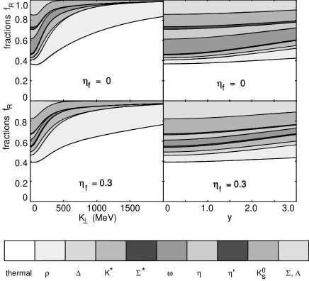
FIG. 1.: The resonance fractions $f_{r}(y,p_{\perp})$ according to Eq. (32) for $T=150$ MeV. Upper row: no transverse flow, $\eta_{f}=0$; lower row: $\eta_{f}=0.3$. Left column: $f_{r}$ as a function of transverse momentum at central rapidity; right column: $f_{r}$ as function of rapidity at $p_{\perp}=0$.

In cases (ii) and (iii) the space-time variances calculated from Eq. (34) yield misleading or outright wrong results for the width of the correlation function. They give the curvature of the correlator at ${\bf q}=0$:

$$\langle\tilde{x}^{2}\rangle = f_{\rm dir}\langle\tilde{x}^{2}\rangle_{\rm dir}+f_{\rm halo}\langle\tilde{x}^{2}\rangle_{\rm halo}=(1-\epsilon)R_{\rm dir}^{2}+\epsilon R_{\rm halo}^{2}$$ (39)

$$= -{1\over 2}\left.{\partial^{2}C(q)\over\partial q^{2}}\right|_{q=0}\,.$$ (40)

In case (ii), for not too small values of $\epsilon$, this is dominated by the second term although the resonance contribution is not even visible in the measured correlator! On a quantitative level, the situation is not very much better for case (iii) (see Sec. VI A 1 for a more detailed discussion).

However, if the resonances can be clearly separated into two distinct classes, one with very short lifetimes of order 1 fm/$c$, the other with very long lifetimes of order 100 fm/$c$ or longer, then space-time variances can again provide an accurate measure for the width of the correlation function. To achieve this, one must leave out the long-lived resonances from the sum over $r$ in (34), i.e. one restricts the calculation of the space-time variances to the “core” of the emission function from direct pions and short-lived resonances [30, 31]. Since the contribution from long-lived resonances to the correlator cannot be resolved experimentally (while they do contribute to the single-particle spectra), one includes them via a reduced correlation strength $\lambda$:

$$\lambda(K)=\left(1-\sum_{r={\rm longlived}}f_{r}(K)\right)^{2}\,.$$ (41)

The $K$-dependence of $\lambda$ will be discussed in Sec. V.

The real problem comes from resonances with an intermediate lifetime. They cause appreciable deviations from a Gaussian behaviour for the correlator and cannot be reliably treated by the method of space-time variances. In nature there is only one such resonance, the $\omega$ meson with its 23.4 fm/$c$ lifetime. At low $K_{\perp}$ it contributes up to 10% of all pions ($f_{\omega}({\bf K}=0)\approx 0.1$), and their non-Gaussian effects on the correlator can be clearly seen. They will be discussed extensively in Sections VI,VII.

IV A simple model for the emission function

As discussed after Eq. (6), a completely model-independent HBT analysis is not possible. In this Section we define a simple model for the emission function in relativistic nuclear collisions which will be used in the rest of the paper for quantitative studies. It has been used extensively in the literature [9, 10, 11, 12, 13, 23], and we present a simple extension to include resonance production. It implements the essential features expected from sources created in nuclear collisions: It assumes local thermalization prior to freeze-out and incorporates its collective expansion in the longitudinal and transverse directions. On the geometric side, the source has a finite size in the spatial and temporal directions, i.e. it implements a finite, but non-zero duration for particle emission.

The emission function for particle species $r$ is taken as

$$S^{\rm dir}_{r}(x,P) = {2J_{r}+1\over(2\pi)^{3}}\,M_{\perp}\cosh(Y-\eta)$$ (43)

$$\times\exp\left(-{P\cdot u(x)-\mu_{r}\over T}\right)\,H(x)$$

where

$$H(x)={1\over\pi(\Delta\tau)}\,\exp\left(-{r^{2}\over 2R^{2}}-{(\eta-\eta_{0})^{2}\over 2(\Delta\eta)^{2}}-{(\tau-\tau_{0})^{2}\over 2(\Delta\tau)^{2}}\right)\,,$$ (44)

with proper time $\tau=\sqrt{t^{2}-z^{2}}$ and space-time rapidity $\eta=\textstyle{1\over 2}\log{[{(t+z)/(t-z)}]}$. The physical meaning of the parameters has been explained in detail in Refs. [9, 10, 11, 12, 13, 23] to which we refer the reader. The only new ingredients are a factor $2J_{r}+1$ for the spin degeneracy (due to charge identification in the experiment each isospin state must be treated separately), and a chemical potential $\mu_{r}$ for each resonance $r$. This means that all particles are assumed to freeze out with the same geometric characteristics and the same collective flow, superimposed by thermal motion with the same temperature. The possible consequences of particle-specific freeze-out [34, 35] will have to be discussed elsewhere.

For later reference we note that the function $H(x)$ is normalized to the total comoving 3-volume according to

$$\int d^{4}x\,H(x) = \pi r^{2}_{\rm rms}\cdot 2\tau_{0}\eta_{\rm rms}\,,$$ (45)

$$r^{2}_{\rm rms}=2R^{2}=x^{2}_{\rm rms}+y^{2}_{\rm rms}\,, \qquad\eta_{\rm rms}=\Delta\eta\,.$$ (46)

Note that the rms widths in $x$- and $y$-direction are each given by $R$. If the Gaussians in $H(x)$ were replaced by box functions [32, 33], the equivalent box dimensions (with the same rms radii) would be $\tilde{R}=2R$, $\tilde{\eta}=\sqrt{3}\,\Delta\eta$.

For the flow profile we assume [12] Bjorken scaling in the longitudinal direction, $v_{l}=z/t$, and a linear transverse flow rapidity profile [36]:

$$\eta_{t}(r)=\eta_{f}{r\over R}\,.$$ (47)

In spite of the longitudinal boost-invariance of the flow, the source as a whole is not boost-invariant due to the finite extension in $\eta$ provided by the second Gaussian in (43).

Inserting the parametrization (A9) for $P$ the emission function (43) becomes [13]

$$S_{r}^{\rm dir}(x,P) = {2J_{r}+1\over(2\pi)^{3}}\,M_{T}\cosh(Y-\eta)\,e^{\mu_{r}/T}\,H(x)$$ (50)

$$\times\exp\left(-{M_{T}\over T}\cosh(Y-\eta)\cosh\eta_{t}(r)\right.$$

$$\qquad\left.+{P_{T}\over T}\sinh\eta_{t}(r)\cos(\phi-\Phi)\right)\,.$$

The direct pion component $S_{\pi}^{\rm dir}(x,p)$ is obtained from this expression by setting $r=\pi$, $P=p$, $J_{\pi}=0$, $\mu_{\pi}=0$, and $\Phi=0$ (see (A7)). This last condition reflects a choice for the orientation of the coordinate system such that the transverse momentum ${\bf p}_{\perp}$ of the decay pion lies in the $x-z$ plane. For the transverse momentum ${\bf P}_{\perp}$ of resonances which contribute pions with the same ${\bf p}_{\perp}$ as the directly emitted ones, in general a non-vanishing azimuthal angle $\Phi$ is required, see Appendix A.

The chemical potentials $\mu_{r}$ will be fixed by the assumption of chemical equilibrium at freeze-out. Then baryon number and strangeness conservation in the fireball demand the existence of two independent chemical potentials $\mu_{B}$ and $\mu_{S}$, with

Decay channel $r$	$M$ (MeV)	$\Gamma$ (MeV)	$J$	$b_{r\to\pi^{-}}$
$\rho^{-}\to\pi^{-}\pi^{0}$	770	150	1	1.0
$\rho^{0}\to\pi^{-}\pi^{+}$	770	150	1	1.0
$\Delta^{-}\to\pi^{-}n$	1232	115	3/2	1.0
$\Delta^{0}\to\pi^{-}p$	1232	115	3/2	$(1/3)\times 1.0$
$\bar{\Delta}^{+}\to\pi^{-}\bar{n}$	1232	115	3/2	$(1/3)\times 1.0$
$\bar{\Delta}^{++}\to\pi^{-}\bar{p}$	1232	115	3/2	1.0
${K^{*}}^{0}\to\pi^{-}K^{+}$	892	50	1	$(2/3)\times 1.0$
${K^{*}}^{-}\to\pi^{-}K^{0}$	892	50	1	$(2/3)\times 1.0$
${\Sigma^{*}}^{-}\to\pi^{-}\Lambda(1116)$	1385	36	1/2	0.88
${\Sigma^{*}}^{-}\to\pi^{-}\Sigma^{0}(1193)$	1385	36	1/2	$(1/2)\times 0.12$
${\Sigma^{*}}^{0}\to\pi^{-}\Sigma^{+}(1193)$	1385	36	1/2	$(1/2)\times 0.12$
$\bar{\Sigma}^{*}{}^{+}\to\pi^{-}\bar{\Lambda}(1116)$	1385	36	1/2	0.88
$\bar{\Sigma}^{*}{}^{+}\to\pi^{-}\bar{\Sigma}^{0}(1193)$	1385	36	1/2	$(1/2)\times 0.12$
$\bar{\Sigma}^{*}{}^{0}\to\pi^{-}\bar{\Sigma}^{-}(1193)$	1385	36	1/2	$(1/2)\times 0.12$
$\omega\to\pi^{-}\pi^{+}\pi^{0}$	782	8.43	1	0.89
$\eta\to\pi^{-}\pi^{+}\pi^{0}$	547	$1.2\times 10^{-3}$	0	0.24
$\eta^{\prime}\to\pi^{+}\pi^{-}\eta$	958	0.2	0	0.44
$K_{S}^{0}\to\pi^{+}\pi^{-}$	498	$\approx 0$	0	$0.69$
$\Sigma^{-}\to\pi^{-}n$	1193	$\approx 0$	1/2	$1.0$
$\bar{\Sigma}^{+}\to\pi^{-}\bar{n}$	1193	$\approx 0$	1/2	$1.0$
${\Sigma}^{0}\to\gamma\Lambda\to p\pi^{-}$	1193	$\approx 0$	1/2	$0.65$
$\Lambda\to p\pi^{-}$	1116	$\approx 0$	1/2	$0.65$

TABLE I.: The resonance decay contributions to $\pi^{-}$ production considered in the present work. Where applicable the factor in front of the branching ratio is the Clebsch-Gordon coefficient for the particular decay channel.

$$\mu_{r}=b_{r}\mu_{B}+s_{r}\mu_{S}\,,$$ (51)

where $b_{r}$ and $s_{r}$ are the baryon number and strangeness of resonance $r$, respectively. The condition of overall strangeness neutrality of the fireball allows to eliminate $\mu_{S}$ in terms of $T$ and $\mu_{B}$ [37].

Unless stated otherwise, the numerical calculations [44] below are done with the set of source parameters $T=150$ MeV, $R=5$ fm, $\Delta\eta=1.2$, $\tau_{0}=5$ fm/c, $\Delta\tau=1$ fm/c and $\mu_{B}=\mu_{S}=0$. We will work in the fireball c.m. system and thus set $\eta_{0}=0$.

The resonance channels included are listed in Table I. The $\Sigma$(1193) and $\Lambda$(1116) are treated as one baryonic resonance $Y$(1150) at an average mass of 1150 MeV. For simplicity the decay cascade $\Sigma^{0}\to\gamma\Lambda\to p\pi^{-}$ is replaced by an effective two-particle decay $\Sigma^{0}\to p\pi^{-}$, since the photon in the $\Sigma^{0}$-decay is known not to change the shape of the hyperon spectrum [32]. The $\pi^{-}$ decay contributions from the cascades $\eta^{\prime}\to...$ $+\eta\to\pi^{-}+...$ and $\Sigma^{*}\to...+$ $Y(1150)\to\pi^{-}+...$ are taken into account by enhanced branching ratios for the $Y$ and $\eta$ decay channels. These crude approximations are not problematic because they concern quantitatively small contributions. The cascade decays just mentioned affect the intercept parameter on the level of a few percent; the ${\bf K}$- dependence of the HBT radius parameters remains essentially unaffected. $K_{L}^{0}$ decays are neglected because the long $K_{L}^{0}$ lifetime ($c\tau$ = 15.5 m) makes them invisible for most detectors.

V Results for one- and two-particle spectra

We now present a quantitative analysis of the one- and two-particle spectra for the model described in Sec. IV. Both types of spectra can be expressed in terms of the four-dimensional Fourier transforms of the direct emission functions, $\tilde{S}_{r}^{\rm dir}(q,P^{\pm})$, see Appendix A. We show in Appendix B how the latter can be reduced analytically to 2-dimensional integrals over $r$ and $\eta$:

$$\tilde{S}_{r}^{\rm dir}(q,P^{\pm}) = {(2J_{r}+1)\over\pi(2\pi)^{3/2}}\,M_{\perp}\,\tau_{0}\,e^{{\mu_{r}\over T}}\int d\eta\,\left(1+iA_{q}\right)$$ (55)

$$\times\cosh(\eta-Y)\,e^{iA\tau_{0}}\,e^{-{1\over 2}A^{2}(\Delta\tau)^{2}}e^{-{\eta^{2}\over 2(\Delta\eta)^{2}}}\,$$

$$\times\int_{0}^{\infty}r\,dr\,e^{-{r^{2}\over 2R^{2}}}\,e^{-{M_{\perp}\over T}\cosh(\eta-Y)\cosh\eta_{t}}$$

$$\times I_{0}\left(\sqrt{C-iD^{\pm}}\right)\,,$$

where

$$C(r) = {P_{\perp}^{2}\over T^{2}}\sinh^{2}\eta_{t}(r)-r^{2}\,q_{\perp}^{2}\,,$$ (57)

$$D^{\pm}(r) = -2\,r\,{P_{\perp}\over T}\sinh\eta_{t}(r)$$ (59)

$$\times\left(q_{o}\cos\Phi_{\pm}+q_{s}\sin\Phi_{\pm}\right)\,,$$

$$A(\eta) = \left(q^{0}\cosh\eta-q_{l}\sinh\eta\right)\,,$$ (60)

$$A_{q}(\eta) = A(\eta){(\Delta\tau)^{2}\over\tau_{0}}\,.$$ (61)

The Bessel function $I_{0}$ arises from the $\phi$-integration while the terms containing $A$ and $A_{q}$ stem from the $\tau$-integration. Please note that the azimuthal rotation of the resonance transverse momentum ${\bf P}_{\perp}$ relative to the pion transverse momentum ${\bf p}_{\perp}$ (which defines the $x$-axis of our coordinate system) enters only through the combination in brackets in Eq. (59); the latter stems from the scalar product $q\cdot P^{\pm}$, see Eq. (A38). This means that the dependence on $\Phi_{\pm}$ can be shifted from ${\bf P}^{\pm}_{\perp}$ to ${\bf q}_{\perp}$ by a common rotation by the angle $\Phi_{\pm}$:

$$\tilde{S}_{r}^{\rm dir}\left(q^{0},q_{o},q_{s},q_{l};E_{{}_{P}},P_{\perp}\cos\Phi_{\pm},P_{\perp}\sin\Phi_{\pm},P_{{}_{L}}\right)=$$ (62)

$$\qquad\tilde{S}_{r}^{\rm dir}\left(q^{0},q_{o}\cos\Phi_{\pm}+q_{s}\sin\Phi_{\pm},q_{s}\cos\Phi_{\pm}-\right.$$ (63)

$$\qquad\,\,\left.q_{o}\sin\Phi_{\pm},q_{l};E_{{}_{P}},P_{\perp},0,P_{{}_{L}}\right)\,.$$ (64)

Note that this identity does not depend on the model for the emission function. It shows that the resonance decay kinematics leads to a mixing of the sideward and outward $q$-dependencies of the correlation functions that would be obtained from the resonances if one could use them for interferometry directly. This feature is lost in the approximation leading to Eq. (2) in Ref. [18].

For the direct pion contribution, $\Phi_{\pm}$ is to be set to zero in (55), (64).

A The resonance fractions $f_{r}(K)$

The single particle momentum spectrum (1) is the space-time integral over the emission function (23),

$${dN_{\pi}\over\pi\,dy\,dm_{\perp}^{2}}=\int d^{4}x\,S_{\pi}(x,p)=\tilde{S}_{\pi}(q=0;m_{\perp},y).$$ (65)

It is thus given by the Fourier transform (55) of the emission function at zero relative momentum. From this expression it is straightforward to evaluate the resonance fractions $f_{r}(y,m_{\perp})$ of Eq. (32). For later referene they are shown in Fig. 1. At central rapidity and small transverse momentum in our model only about 40% of the pions are emitted directly while more than half of the pions stem from resonance decays. The direct fraction increases rapidly with increasing transverse momentum, but very slowly with increasing longitudinal momentum resp. rapidity. In fact, most resonance fractions are nearly independent of rapidity [8]. At large $p_{\perp}$ the resonance contributions to the single particle spectrum die out [17]. The largest resonance contribution comes from the $\rho$ meson, due to its relatively small mass and large spin degeneray factor. The $\eta$, which is still lighter, has no spin and a small branching ratio into pions. As can be seen in the lower row of Fig. 1 the resonance fractions are only weakly affected by transverse flow: at small $p_{\perp}$ the direct fraction increases slightly while at large $p_{\perp}$ the tendency is opposite (see Sec. V B).

B Single particle transverse momentum spectra

Integrating (65) over rapidity we obtain the single particle transverse momentum distribution:

$${dN_{\pi}\over dm_{\perp}^{2}} = \pi\int dy\,\tilde{S}_{\pi}^{\rm dir}(0;y,m_{\perp})$$ (67)

$$+\sum_{r\neq\pi}\pi\int dy\,\tilde{S}_{r\to\pi}(0;y,m_{\perp})\,.$$

The resonance decay contributions are given according to Eqs. (A34) and (A38) by

$$\tilde{S}_{r\to\pi}(0;y,m_{\perp})=2M\int_{\bf R}S_{r}^{\rm dir}(0;Y,M_{\perp})\,.$$ (68)

The factor 2 results from the sum over $\Phi_{\pm}$, noting that at $q=0$ the integrand is independent of $\Phi_{\pm}$ (see Appendix B). Writing $Y=y+v\Delta Y$ (see Eq. (A31)) where $\Delta Y$ is independent of $y$, the $y$-integration can be pulled through the integrals $\int_{\bf R}$ over the decay phase space, yielding [17]

$${dN_{\pi}\over dm_{\perp}^{2}}={dN_{\pi}^{\rm dir}\over dm_{\perp}^{2}}+\sum_{r\neq\pi}2M_{r}\int_{\bf R}{dN_{r}^{\rm dir}\over dM_{\perp}^{2}}\,.$$ (69)

The transverse momentum spectra of the directly emitted resonances $r$ are given by expression (B18) [17, 32]:

$${dN_{r}^{\rm dir}\over dM_{\perp}^{2}} = {2J_{r}+1\over 4\pi^{2}}\,(2\pi R^{2}\cdot 2\tau_{0}\Delta\eta)\,e^{\mu_{r}/T}$$ (72)

$$\times\,M_{\perp}\int_{0}^{\infty}d\left({\xi^{2}\over 2}\right)e^{-\xi^{2}/2}\,K_{1}\left({\textstyle{M_{\perp}\over T}}\cosh\eta_{t}(\xi)\right)$$

$$\times\,I_{0}\left({\textstyle{P_{\perp}\over T}}\sinh\eta_{t}(\xi)\right)\,,$$

where we substituted $\xi=r/R$ under the integral. Note that the geometric parameters $R$, $\Delta\eta$, $\tau_{0}$ of the source enter only in the normalization of the spectrum through the effective volume (45). Thus the shape of the ($y$-integrated!) single-particle transverse momentum spectrum contains no information on the source geometry, in agreement with general arguments presented e.g. in [12]. According to (69,72), the unnormalized transverse momentum dependence is fully determined by the rest mass $M$, the temperature $T$ (or $T(\xi)$ if $T$ were $r$-dependent), and the transverse flow profile $\eta_{t}(\xi)=\eta_{f}\xi^{n}$.

For later reference we plot in Fig. 2 the pion transverse mass spectrum for the two sets of source parameters for which we compute two-particle correlations below. All resonance decay contributions are shown separately. The only 3-body decays are those of the $\omega$, $\eta$ and $\eta^{\prime}$ whose decay pions are seen to be particularly concentrated at small $p_{\perp}$. (A similar low-$p_{\perp}$ concentration occurs for pions from $K_{S}^{0}$ decays, due to the small decay phase space in this particular 2-body decay.) Comparing the top panel (no transverse flow, $\eta_{f}=0$) with the bottom panel ($\eta_{f}=0.3$) one observes the well-known flattening of the transverse mass spectrum by transverse radial flow [32, 33, 34, 38]. The direct pions reflect essentially an effective “blueshifted” temperature $T_{\rm eff}=T\sqrt{{1+\langle\beta_{t}\rangle\over 1-\langle\beta_{t}\rangle}}$ [38]. But the heavier resonances, in the region $P_{\perp}<M_{r}$, are affected much more strongly by transverse flow since at small $P_{\perp}$ the flattening of the spectra by flow is proportional to the particle rest mass [34, 38].

FIG. 2.: The single pion transverse mass spectrum for $T=150$ MeV and $\mu_{B}=\mu_{S}=0$. The overall normalization is arbitrary, the relative normalizations of the various resonance contributions are fixed by the assumption of thermal and chemical equilibrium. Upper panel: no transverse flow, $\eta_{f}=0$; lower panel: $\eta_{f}=0.3$.

Fig. 2b shows that this effect on the parent resonances is also reflected in the spectra of the daughter pions, explaining the slight rise with $\eta_{f}$ of the resonance fractions at large $m_{\perp}$. This flattening of the transverse mass spectra by transverse flow, suggested in Refs. [38, 32, 33] as an explanation for the observed features of the single particle spectra from ²⁸Si- and ³²S-induced collisions at the AGS and SPS, seems to have been confirmed by recent collision experiments with very heavy ions (Au+Au at the AGS, Pb+Pb at the SPS, see contributions by Y. Akiba, R. Lacasse, Nu Xu and P. Jones at the recent Quark Matter ’96 conference [39]). One of the main goals of two-particle interferometry is to obtain an independent and more direct measure of the transverse expansion velocity at freeze-out, to confirm this picture and further discriminate against possible alternative explanations.

FIG. 3.: The two-particle correlator $C({\bf q},{\bf K})$ for $\pi^{-}$ pairs with pair rapidity $Y=0$ in the CMS. Each row of diagrams corresponds to a different value for the transverse pair momentum $K_{\perp}$ ($K_{\perp}=0,200,400,600$ and 800 MeV from top to bottom). Left column: the correlator in the outward direction at $q_{s}=q_{l}=0$. Middle column: the correlator in the sideward direction at $q_{o}=q_{l}=0$. Right column: the correlator in the longitudinal direction at $q_{s}=q_{o}=0$. Source parameters as in Sec. IV, the transverse flow $\eta_{f}$ has been set to zero.
Here and in the following plots the different lines have the following meaning: Thin solid line: thermal pions only. Long-dashed: including additionally $\rho$-decays. Short-dashed: including additionally all other shortlived resonances ($\Delta,K^{*},\Sigma^{*}$, see Table I). Dash-dotted: adding also $\omega$-decays. Thick solid line: adding also all longlived resonances ($\eta,\eta^{\prime},K_{S}^{0},\Sigma,\Lambda$, see Table I).

C Two-particle correlations

In Figs. 3 and 4 we plot the two-pion correlator $C({\bf q},{\bf K})$ in the three Cartesian directions of ${\bf q}$ for zero and non-zero transverse flow $\eta_{f}$, respectively. We use the letter $Y$ to denote the rapidity of the pair, and $K_{\perp}$ ($M_{\perp}$) for its transverse momentum (transverse mass). The pion pairs in Figs. 3 and 4 have pair rapidity $Y=0$ in the CMS, and transverse momenta ranging from 0 to 800 MeV/$c$ (top to bottom). The correlation functions were calculated by numerically evaluating Eq. (27) for the source parameters given in Sec. IV.

FIG. 4.: Same as Fig. 3, but for nonzero transverse flow $\eta_{f}=0.3$.

Within each plot, the different lines show the effect of adding in Eq. (27) in the sum over decay channels $r$ successively more resonances (see Table I): first the abundant $\rho$, then the other short-lived resonances, then the $\omega$ with its intermediate lifetime, and finally all the long-lived resonances. Comparing these plots row by row gives one a feeling for the $K_{\perp}$-dependence of the correlation function and the various resonance contributions. In the following two subsections we give a rough and general discussion of the main features of the correlator without and with transverse flow of the source, respectively, before proceeding to a quantitative analysis in Sec. VI.

1 No transverse flow (Fig. 3)

The direct thermal contribution leads to a correlation function with a nearly Gaussian shape in all directions $q_{i}$, $i=o,s,l$, and for all pair momenta $K_{\perp}$. As $K_{\perp}$ increases, the correlator becomes rapidly wider in the longitudinal direction while in the two transverse directions the changes are hard to see and require a finer analysis (Sec. VI). As more and more of the short-lived resonances are added, the width of the correlator becomes smaller, again with a larger effect in the longitudinal than in the two transverse directions. A much stronger effect is caused by the $\omega$-meson; now the narrowing of the correlation function is also clearly seen in the transverse directions, and the correlator becomes markedly non-Gaussian. As the long-lived resonances are added, the intercept $\lambda$ of the correlator at ${\bf q}=0$ decreases below 1. This is a matter of $q$-resolution (we stop at $|{\bf q}|=1$ MeV) – the contribution from the long-lived resonances is entirely concentrated in a $\delta$-function like structure near the origin, and with infinite resolution the correlator could be seen to actually reach the value 1 at ${\bf q}=0$. This is, of course, an extreme deviation from Gaussian behaviour.

Long-lived resonances thus lead to apparently incomplete correlations, $\lambda<1$ [8, 15]. This effect becomes even stronger, if the correlator is projected onto one particular $q$-direction by averaging over a finite window in the other directions where the correlator has already dropped below $\lambda$ [40].

As the pion pair momentum $K_{\perp}$ increases, all resonance effects on the width and strength of the correlator are seen to decrease. This is a direct consequence of the decreasing resonance fractions, see Fig. 1.

The above lifetime hierarchy of resonance effects can be understood in terms of the following simple picture:

• Short-lived resonances, $\Gamma>30$ MeV. In the rest frame of the particle emitting fluid element these resonances decay very close to their production point, especially if they are heavy and have only small thermal velocities. This means that the emission function $S_{r\to\pi}$ of the daughter pions has a very similar spatial structure as that of the parent resonance, $S_{r}^{\rm dir}$, although at a shifted momentum and shifted in time by the lifetime of the resonance. As only $R_{o}$ and $R_{l}$ are sensitive to the lifetime of the source, the shift in time affects the correlation function only in the outward and longitudinal directions. The stronger effect on $R_{l}$ (which is obvious from the right column in Fig. 3) is a consequence of the boost-invariant longitudinal expansion of our source: as the decay pions are emitted at a later proper time $\tau$, and since the longitudinal length of homogeneity increases with $\tau$ because the longitudinal velocity gradients decrease [10], the decay pions show a larger longitudinal homogeneity length than the direct pions. – Since the Fourier transform of the direct emission function is rather Gaussian and the decay pions from short-lived resonances appear close to the emission point of the parent, they maintain the Gaussian features of the correlator.

• Long-lived resonances, $\Gamma\ll 1$ MeV. These are the $\eta$ and $\eta^{\prime}$, with lifetimes $c\tau_{\Gamma}\approx 17.000$ and 1000 fm, respectively, and the weak decays of $K_{S}^{0}$ and the hyperons which on average propagate several cm. (The decays of $K_{L}^{0}$ and charged kaons are not included in our calculation because they are reconstructed in most experiments.) Even with thermal velocities these particles travel far outside the direct emission region before decaying, generating a daughter pion emission function $S_{r\to\pi}$ with a very large spatial support. The Fourier transform $\tilde{S}_{r\to\pi}(q,K)$ thus decays very rapidly for $q\neq 0$, giving no contribution in the experimentally accessible region $q>1$ MeV. (This lower limit in $q$ arises from the finite two-track resolution in the experiments.) The decay pions do, however, contribute to the single particle spectrum $\tilde{S}_{r\to\pi}(q=0,K)$ in the denominator and thus “dilute” the correlation. In this way long-lived resonances decrease the correlation strength $\lambda$ without, however, affecting the shape of the correlator where it can be measured.

• Moderately long-lived resonances, $1$ MeV $<\Gamma<30$ MeV. There is only one such resonance, the $\omega$ meson. It is not sufficiently long-lived to escape detection in the correlator, and thus it does not affect the intercept parameter $\lambda$. Its lifetime is, however, long enough to cause a long exponential tail in $S_{\omega\to\pi}(x,K)$. This seriously distorts the shape of the correlator and destroys its Gaussian form.

2 Non-zero transverse flow (Fig. 4)

The main difference between Figs. 3 and 4 is that the effects from the short-lived resonances and the $\omega$ on the shape of the correlator are weaker. The primary reason for this behaviour is that for the class of models (50) the transverse size $R_{t}$ of the effective emission region for heavy resonances shrinks for nonzero transverse flow. In Gaussian saddle point approximation, this transverse size $R_{t}$ can be calculated from $S_{r}^{\rm dir}(x,P)$ in (50) as

$$R_{t}={R\over\sqrt{1+(M_{\perp}/T)\eta_{f}^{2}}}\,.$$ (73)

This is not accurate enough for quantitative studies [11] but gives the correct tendency and right order of magnitude. Going like $\eta_{f}^{2}$ this effect is small, but it tends to increase the width of the correlator, counteracting the basic tendency of resonance contributions to make the correlator narrower. For $\eta_{f}=0.3$ the two effects are seen to more or less balance each other in the sideward correlator, leaving practically no trace of the shortlived resonances including the $\omega$. A similar effect is seen in the outward and longitudinal directions, but there the dominant lifetime effect discussed above prevails.

Please note that none of the correlators shown in Figs. 3,4 exhibits a “volcanic” (exponential or power law rather than Gaussian) shape as seen for the longitudinal correlators of Refs. [8]. We have not been able to trace the origin of this discrepancy; it may be due to the different source (hydrodynamics with freeze-out along a sharp hypersurface) used in Refs. [8], but why this should manifest itself in this way is not obvious. From general arguments we would expect at small $q$ a Gaussian behaviour with a curvature related to the longitudinal size of the effective pion source from $\omega$ decays; the longitudinal correlators in Refs. [8] seem to decay much more steeply for small $q$. We have checked our results with two independent programs, based on the formulae given in the Appendices.

VI Extracting HBT-radii from the correlator

Looking at Figs. 3 and 4 it is clear that more quantitative methods are needed to characterize the shape of the correlator. For an interpretation of the correlator in terms of the space-time structure of the source relatively small changes of its shape and its pair momentum dependence play an important role. One would therefore like to describe the key features of $C({\bf q},{\bf K})$ by a small number of fit parameters which are sensitive to this space-time structure. The usual procedure is to perform a Gaussian fit with the functions (8) or (15). As we will see this method runs into systematic problems if the 2-particle correlator does not have a perfect Gaussian shape, e.g. due to long-lived resonances. Not only do the functions (8) or (15) fail to give a good fit, but by not correctly accounting for the non-Gaussian features one throws away important space-time information contained in the resonance decay contributions to the correlator.

In this Section we discuss several different Gaussian fitting procedures which clearly demonstrate these difficulties. The main reason for presenting this basically flawed approach is (i) that it is the method mainly used so far in the experimental analysis and (ii) that the discussion throws some light on how one should compare HBT radius parameters extracted by different groups using different procedures. After having understood the problems and the systematic uncertainties they generate we will then suggest a more reliable approach in the next Section which also accounts for non-Gaussian features in a quantitative way.

A Two-dimensional Gaussian fits to the correlator

We start by discussing 2-dimensional fits to $C({\bf q},{\bf K})$ with two parameters $\lambda_{i}(K)$, $R_{i}(K)$ ($i=o,s,l$). We approximate the numerical function in the directions $q_{i}$ as follows:

$$C(q_{i},q_{k\neq i}=0;{\bf K})\approx 1+\lambda_{i}({\bf K})\,e^{-R_{i}^{2}({\bf K}){q_{i}}^{2}}\,,\quad i=o,s,l\,.$$ (74)

The optimal parameters $\lambda_{i}({\bf K})$ and $R_{i}({\bf K})$ are determined by minimizing the following expression:

$$\sum_{\nu=1}^{n}\left(\ln C(q_{i}^{\nu},q_{k\neq i}=0;{\bf K})-\ln\lambda_{i}+R_{i}^{2}(q_{i}^{\nu})^{2}\right)^{2}={\rm min}\,.$$ (75)

FIG. 5.: The Cartesian HBT radii $R_{i}$, $i=o,s,l$ and their corresponding intercept parameters $\lambda_{i}$, extracted from the correlator $C({\bf q},{\bf K})$ via 2-dimensional fits according to Eq. (75). Shown are results at $Y=0$ as function of $K_{\perp}$ for $\eta_{f}=0$. Top row: sideward direction. Middle row: outward direction. Bottom row: longitudinal direction. The different lines indicate the effects of including various sets of resonances as described in Fig. 3.

The label $\nu$ runs over a set of $n$ equidistant values $q_{i}^{\nu}$ between $0$ and $50$ MeV for which the correlator $C(q_{i}^{\nu},{\bf K})$ was calculated numerically. Although the procedure (75) is conceptually different from an experimental fitting procedure in that the function to be fitted is known exactly and the resulting optimal fit parameters thus don’t have statistical error bars, they can still vary systematically depending on the selection of the fit points $q_{i}^{\nu}$ and the minimization function (75). These systematic variations reflect the possible non-Gaussian features of the correlator, but not in a way that allows to easily quantify them. As long as the deviations from Gaussian bahavior are small, the extracted Gaussian fit parameters $R_{i}({\bf K})$ and $\lambda_{i}({\bf K})$ are expected to be useful for a simple characterization of the main features of the correlator.

1 No transverse flow

For the case $\eta_{f}=0$ the results from independent 2-dimensional fits to the correlator in the “side” (top), “out” (middle), and “long” (bottom) directions are shown in Fig. 5. The left column shows the Cartesian HBT radii, the right column the associated intercept parameters resulting from the fit, both as functions of $K_{\perp}$ at $Y=0$.

The fitted intercept parameters follow roughly the behaviour expected from Eq. (41) and Fig. 1. Upon closer inspection one sees, however, that also some of the shorter-lived resonances, in particular the inclusion of the $\omega$, have a significant lowering effect on $\lambda$. These effects are different in the three Cartesian directions and strongest in the longitudinal direction, where even without any resonance effects $\lambda<1$ at small $K_{\perp}$.

The deviations of the intercept parameter from unity reflect non-Gaussian features of the correlator. For short-lived resonances these are weak, except in the longitudinal $q_{l}$-direction where the correlator has been known to show at small $K_{\perp}$ a somewhat steeper than Gaussian fall-off due to the rapid boost-invariant longitudinal expansion of the source [11], even in the absence of resonance decays. The main non-Gaussian effects come from the $\omega$ and, of course, from the long-lived resonance. The latter affect, however, only $\lambda$ and not the HBT radii extracted from the Gaussian fit, while the $\omega$ also changes the radius parameters.

The fit accomodates these non-Gaussian features by lowering the intercept $\lambda$. As discussed in Sec. V C the main origin of non-Gaussian effects due to resonances is the tail in the time-distribution of the decay pions. According to Eqs. (2.7) this is expected to affect $R_{o}$ and $R_{l}$, but not $R_{s}$. Eq. (5.3) tells us, however, that the “out” and “side”-behaviour of the parent resonance distribution gets mixed in the pair distribution of the daughter pions, so some fraction of this effect propagates into the side-correlator of the decay pions. On the other hand there remains the fact that, compared to $R_{s}$, in $R_{o}$ an additional lifetime effect comes in through the term $\beta_{\perp}^{2}\langle\tilde{t}^{2}\rangle$ in (11); this contribution increases quadratically for small values of $K_{\perp}$, saturating above $K_{\perp}=m_{\pi}$ where $\beta_{\perp}\approx 1$. This explains very nicely the initial drop and subsequent rise of $\lambda$ in the outward direction, which is particularly prominent for the $\omega$ contribution.

Let us now turn our attention to the HBT radii in the left column of Fig. 5 and begin with a discussion of $R_{s}$. Its size remains essentially unaffected by the short-lived resonances with lifetimes of order $1$ fm/$c$, but the $\omega$ affects $R_{s}$. This effect dies out rapidly for increasing $M_{\perp}$ due to the decreasing $\omega$-fraction $f_{\omega}(K_{\perp},0)$, but the resulting $M_{\perp}$-dependence of $R_{s}$ complicates the extraction of the transverse flow from it [11, 13].

The origin of the effect has already been qualitatively explained in Sec. V C and above by referring to Eq. (64). A somewhat more quantitative estimate can be obtained by studying the space-time variances of Sec. III, even though the discussion presented there makes it clear that this will provide only an upper estimate for the $\omega$-contribution to $R_{s}$. Considering only the direct pions and those from $\omega$-decays and calculating $R_{s}^{2}=\langle y^{2}\rangle$ according to (34) we find

$${\langle{y^{2}}\rangle}=f_{\rm dir}{\langle{y^{2}}\rangle}_{\rm dir}+f_{\omega}{\langle{y^{2}}\rangle}_{\omega}$$ (76)

with

$${\langle{y^{2}}\rangle}_{\omega} = {{\int d^{4}x\,\sum_{\pm}\int_{\bf R}\int_{0}^{\infty}d\tau\Gamma\,e^{-\tau\Gamma}y^{2}\,S_{\omega}^{\rm dir}{\left(x-{P^{\pm}\over M}\tau,P^{\pm}\right)}}\over\int d^{4}x\,\sum_{\pm}\int_{\bf R}\int_{0}^{\infty}d\tau\Gamma\,e^{-\tau\Gamma}S_{\omega}^{\rm dir}{\left(x-{P^{\pm}\over M}\tau,P^{\pm}\right)}}$$ (78)

$$= R^{2}+{\left({1\over\Gamma^{2}}\right)}f_{\rm corr}\,,$$ (79)

$$f_{\rm corr} = 2\,{{\int_{\bf R}{P_{\perp}^{2}\over M^{2}}\int d^{4}xS_{\omega}^{\rm dir}(x,P^{\pm})\,\sin^{2}\Phi_{\pm}}\over{\int_{\bf R}\int d^{4}x\,S_{\omega}^{\rm dir}(x,P^{\pm})}}\,.$$ (80)

Using $f_{dir}+f_{\omega}=1$ this yields

$${\langle{y^{2}}\rangle}=R^{2}+f_{\rm corr}\,f_{\omega}\,{1\over\Gamma^{2}}\,.$$ (81)

This result can be explained as the effect of the $\omega$ propagating in the $y$-direction before decaying or, more formally, as the effect of the “out”-“side”-mixing in the decay kinematics expressed by Eq. (64). Numerically, we determined the factor $f_{\rm corr}\approx 0.52$ at $K_{\perp}=0$ which leads to $f_{\rm corr}\cdot f_{\omega}\approx 0.1$ at the same point. Putting this together with the width of the $\omega$-resonance, ${1\over\Gamma}=23.4$ fm, one obtains for the side variance $\sqrt{{\langle{y^{2}}\rangle}}=8.9$ fm.

This is obviously much larger than the $5.5$ fm extracted at $K_{\perp}=0$, since the curvature (22) does not coincide with the fitted width. For longer living resonances this discrepancy will, of course, be even larger. Another number to compare with is the half width $R_{s}^{\rm half}$ of the correlator $C(q_{s})$ at $q_{o}{=}q_{l}{=}{\bf K}{=}0$, including all short-lived resonances plus the $\omega$. We find the hierarchy

$$\sqrt{{\langle{y^{2}}\rangle}}\approx 8.9\text{ fm}>R_{s}^{\rm half}\approx 6.4\text{ fm}>R_{s}\approx 5.5\text{ fm}\,.$$ (82)

We conclude that estimates of resonance effects, based on space-time variances like $\sqrt{{\langle{y^{2}}\rangle}}$, as e.g. done in [18], are quantitatively unreliable. The half width $R_{s}^{\rm half}$ is close to the result one would obtain from a Gaussian fit to the correlator when the intercept $\lambda$ is fixed to the value of (41) (as e.g. done, albeit simultaneously in all three $q$-directions, in Refs. [8, 41]). The difference to our procedure which lets $\lambda$ float is significant, and since $C$ at ${\bf q}=0$ is not experimentally accessible, a comparison of $R_{s}^{\rm half}$ with data [41] is clearly dangerous. The authors of Refs. [8] also find that at low $K_{\perp}$ resonance decays can increase the longitudinal HBT radius $R_{l}$ by up to a factor 2; in a Gaussian fit with floating $\lambda$ we never see resonance induced increases in $R_{l}$ by more than 1.5 fm.

FIG. 6.: The correlator $C(q_{s})$ at $q_{o}{=}q_{l}{=}{\bf K}{=}0$, taking into account only direct pions and pions from $\omega$ decays. The upper panel shows the three contributions according to Eq. (27): direct-direct pairs (dashed), direct-direct + direct-$\omega$ (dotted), and all contributions (including the $\omega-\omega$ term where both pions come from $\omega$ decays) (solid line). The lower panel compares the same solid line to different Gaussians whose radius parameters correspond to the curvature at $q_{s}=0$ (dotted line), the half width of $C(q_{s})$ (dash-dotted line), and the optimal Gaussian fit according to Eq. (75) (dashed line).

We have compared the Gaussians corresponding to the numbers given in Eq. (82) with the true “side”-correlator in the lower panel of Fig. 6. In the upper panel we show the three contributions to the correlator (see (27) and (38)) coming from pairs of two directly emitted pions (dashed line), from pairs of one direct and one $\omega$ decay pion (difference between dotted and dashed lines), and from pairs where both pions come from $\omega$ decays (difference between solid and dotted lines). While it is obvious that the $\omega$ contributions are concentrated at lower $q_{s}$-values than the direct one, the tail from the mixed direct-$\omega$ contribution is still appreciable outside the half-point of the direct term near $q_{s}=30$ MeV. It therefore appears impossible to cleanly separate the correlation function into “core” and “halo” contributions with different $q$-support [15]. In particular, the recent suggestion by Csörgő [31] to extract the “core” radius by performing a Gaussian fit to the $q_{s}$-tail of the correlator, excluding the range $q_{s}<q_{\rm cut}$ where $q_{\rm cut}\sim 30$ MeV, is likely to run into systematic problems.

We now turn to $R_{o}$. At $K_{\perp}=0$ the two transverse radius parameters $R_{s}$ and $R_{o}$ are equal by symmetry [23], and all above considerations carry over to the “out”-direction. At non-zero $K_{\perp}$, $R_{o}$ receives an additional contribution from the source lifetime as indicated by Eq. (11). Although for the $\omega$ the use of this expression is no longer quantitatively reliable, it gives the correct tendency. Short-lived resonances do not destroy the Gaussian shape of the out-correlator, and for them Eq. (11) (with Eq. (34)) can be used without restrictions. It is obvious that even the short-lived resonances contribute through their lifetime to the term $\beta_{\perp}^{2}\langle\tilde{t}^{2}\rangle$ in (11), strengthening the rise of $R_{o}$ in Fig. 5 at small $K_{\perp}$.

The strongest resonance effect is seen for $R_{l}$, which is affected even by the short-lived resonances. These effects disappear for large $K_{\perp}$ due to the decreasing resonance fractions $f_{r}$, but at small $K_{\perp}$ they are significant. Due to the existence of (weak) non-Gaussian features already in the absence of resonances the space-time variances are of limited use for a quantitative discussion of the effects, and we leave the reader with the numerical results shown in Fig. 5. A qualitative interpretation was given in Sec. V C.

2 Non-zero transverse flow

In Fig. 7 we show the parameters $\lambda_{i}$, $R_{i}$ obtained from the 2-dimensional fit (74), (75) for the case of non-zero transverse expansion with $\eta_{f}=0.3$. Comparing with Fig. 5 one sees that the effect of the resonances on the radius on the HBT radius parameters are weaker, and that correspondingly the non-Gaussian effects caused by the short-lived resonances and the $\omega$ (which lead to deviations of the intercept parameter $\lambda$ from unity) are less pronounced. In fact, the only remaining effects of these resonances on the HBT radii come from the terms $\sim\langle\tilde{t}^{2}\rangle$ in $R_{o}$ and $R_{l}$ (see (II)) and are due to the additional contribution to the particle emission duration from the resonance lifetimes. The geometrical effect of resonance propagation away from the direct source, described by the second term in (81), has disappeared, even for the $\omega$. The reason was already discussed in Sec. V C, Eq. (73): due to transverse flow the transverse size of the emission region for heavy resonances is smaller than that of the direct pions, and since they don’t live very long they usually don’t make it outside the source of direct pions before decaying. Thus they don’t lead to an increase of the spatial source size.

FIG. 7.: Same as Fig. 5, but for non-zero transverse flow $\eta_{f}=0.3$.

As a consequence, the decrease of $R_{s}$ with increasing $K_{\perp}$, which is characteristic for transverse collective flow of the source [11, 13], is no longer modified by the pions from $\omega$ decays. This is, of course, the ideal situation one might hope for in order to extract quantitative dynamical information from HBT data. Unfortunately, the problem remains that, if the measurement finds a (not too strong) $M_{\perp}$-dependence of $R_{s}$, it could still be due to either weak transverse flow without resonance contaminations as in Fig. 7, or to $\omega$-decay contributions in the absence of transverse flow as in Fig. 5. (Other mechanisms like transverse temperature gradients might also create an $M_{\perp}$-dependence [9, 10].) We must find a more quantitative analysis tool which allows us to tell whether the $M_{\perp}$-dependence of $R_{s}$ is associated with $\omega$-decays or not.

B Five-dimensional Cartesian Gaussian fits to the correlator

Before approaching this task in the next Section, we will now also discuss some generic features of multi-dimensional Gaussian fits to the exact correlator where all HBT parameters and the correlation strength are determined simultaneously. This is clearly desirable in order to avoid the problem of having three different correlation strengths in the three Cartesian directions, as happens when the three radii $R_{s}$, $R_{o}$, and $R_{l}$ are determined by separate 2-dimensional fits according to (74), because such a result is clearly unphysical. It is also necessary for the determination of the cross-term $R_{ol}$ and for a fit with the YKP parametrization (15).

FIG. 8.: The Cartesian HBT radii $R_{o}$, $R_{s}$, $R_{l}$, and the intercept $\lambda$, obtained from the 5-dimensional fit (84) to $C({\bf q},{\bf K})$, as functions of $K_{\perp}$ at $Y=0$. $R_{ol}$ is not shown since at $Y=0$ it vanishes due to symmetry. Left column: no transverse flow, $\eta_{f}=0$. Right column: $\eta_{f}=0.3$.

In this Subsection we extract the Cartesian parameters $R_{o}$, $R_{s}$, $R_{l}$, $R_{ol}$ and $\lambda$ from a 5-dimensional fit which minimizes the expression

$$\sum_{\nu=1}^{n}\left[\ln C({\bf q}^{\nu},{\bf K})-\ln\lambda+R_{o}^{2}\,(q_{o}^{\nu})^{2}+R_{s}^{2}\,(q_{s}^{\nu})^{2}+R_{l}^{2}\,(q_{l}^{\nu})^{2}\right.$$ (83)

$$\qquad+2\,R_{ol}^{2}\,q_{o}^{\nu}\,q_{l}^{\nu}\Big{)}^{2}=\text{min}.$$ (84)

The label $\nu$ again runs over $n$ fit points ${\bf q}^{\nu}$ which were chosen to lie at equal distances between 0 and 50 MeV along the three Cartesian $q$-axes and along the two diagonals $(q_{s}=0,q_{o}=q_{l})$ and $(q_{s}=0,q_{o}=-q_{l})$. This is, of course, different from a typical experimental ${\bf q}$-distribution. They were selected to economize in the number of fit points where the exact correlator had to be computed.

The results of the fit (84) are shown in Fig. 8, again for $\eta_{f}=0$ and $\eta_{f}=0.3$ at midrapidity $Y=0$. Let us first look at the incercept parameter $\lambda$. Comparing with Figs. 5, 7 we see that the $\lambda$-value from the 5-dimensional fit lies somewhere between the three different values obtained in the 2-dimensional fits. As before it reflects the deviations of the correlator from a Gaussian. Since such deviations exist in the $q_{l}$-direction even without resonances, due to strong longitudinal expansion, $\lambda$ slightly deviates from 1 even in the absence of resonance decays.

The need for the fit to compromise on a unique intercept parameter affects the optimum values for the HBT radius parameters. For a fixed correlation function, a decrease of $\lambda$ leads automatically also to a smaller Gaussian radius as found by the fit. Since the compromise value for $\lambda$ lies above the value $\lambda_{l}$, but below the values $\lambda_{s}$ and $\lambda_{o}$ from the 2-d fits, $R_{l}$ increases and $R_{s}$, $R_{o}$ decrease in the 5-d fit relative to the 2-d fit values. (This effect is hardly visible if resonance decays are switched off but becomes stronger as the resonance contributions (with their non-Gaussian effects) are added.) The net result is that even in the absence of transverse flow now the resonance effects on $R_{s}$ and on its $M_{\perp}$-dependence appear quite weak. Even the resonance contribution to the lifetime effect in $R_{o}$ (the quadratic rise at small $K_{\perp}$) becomes less pronounced.

For completeness we show in Fig. 9 also results at forward pair rapidity $Y=1.5$. In this case the fit gives, of course, a non-vanishing cross-term $R_{ol}$ with the expected $K_{\perp}$-behaviour [42]. It is affected by resonances essentially at the same level as $R_{o}$. The only other qualitative difference is the much smaller value of $R_{l}$ relative to $Y=0$; this is an effect of Lorentz contraction.

It must be stressed that the differences between this Subsection and the previous one are purely due to fit systematics. Depending on how the exact correlator is fitted to a Gaussian the extracted Gaussian radii show significant differences. Since in the experiments the intercept parameter cannot be directly measured and must be fitted simultaneously with the HBT radii, we adopted the same procedure and let $\lambda$ float in the fit. Schlei [8, 41], on the other hand, in his Gaussian fits has always fixed $\lambda$ at the value given by Eq. (41). In the presence of non-Gaussian effects due to resonance decays our fits give smaller $\lambda$’s and, therefore, smaller HBT radii than his fit. This explains why the resonance effects on the transverse radii and their $K_{\perp}$-dependence were found to be much stronger in Refs. [8, 41] than in our work here. According to the second inequality in (82) the difference in $R_{s}$ is about 1 fm, in good agreement with his compared to our results.

FIG. 9.: Same as Fig. 8, but for forward rapidity $Y=1.5$. Now also $R_{ol}$ is non-zero.

C Five-dimensional Gaussian YKP fits to the correlator

The extraction of the Yano-Koonin velocity from a fit according to Eq. (15) is a non-linear problem. To maintain the simplicity of a least-square fit with linear fit parameters we have reformulated the YKP fit problem as follows: We rewrite (15) in the form

$$C({\bf K},{\bf q}) = 1+\lambda_{{}_{\rm YKP}}({\bf K})\exp\left[-R_{\perp}^{2}({\bf K})\,q_{\perp}^{2}-R_{33}^{2}({\bf K})q_{l}^{2}\right.$$ (86)

$$\qquad\left.-R_{00}^{2}({\bf K})(q^{0})^{2}+2R_{03}^{2}({\bf K})q^{0}q_{l}\right]\,,$$

with

$$v = {1\over 2D}\left(1-\sqrt{1-\left({4D^{2}}\right)^{2}}\right)\,,$$ (88)

$$R_{0}^{2} = {{R_{00}^{2}-v^{2}\,R_{33}^{2}}\over{1+v^{2}}}\,,$$ (89)

$$R_{\parallel}^{2} = {{R_{33}^{2}-v^{2}\,R_{00}^{2}}\over{1+v^{2}}}\,,$$ (90)

$$D = {R_{03}^{2}\over{R_{00}^{2}+R_{33}^{2}}}\,.$$ (91)

We then proceed as with the Cartesian parametrization in Sec. VI B, using the same set of fit points as before, but expressing them through their components $q_{\perp},q_{l}$, and $q^{0}$, in order to determine $\lambda_{{}_{\rm YKP}},R_{\perp},R_{33},R_{00}$, and $R_{03}$. Finally we solve Eqs. (VI C) for the YKP parameters.

FIG. 10.: From top to bottom: the YKP fit parameters $R_{\perp}$, $R_{0}$, $R_{\parallel}$, and $\lambda_{{}_{\rm YKP}}$ as functions of $K_{\perp}$ at mid rapidity $Y=0$. Left column: no transverse flow, $\eta_{f}=0$. Right column: $\eta_{f}=0.3$. At $Y=0$ the Yano-Koonin velocity $v$ vanishes exactly.

However, the one-to-one correspondence between the YKP and Cartesian radius parameters does not imply that in a fit to experimental data both sets of fit parameters can be determined with similar accuracy. At mid rapidity, for instance, where $q^{0}=\beta_{\perp}\,q_{o}$, the YKP fit becomes for small transverse pair momentum increasingly insensitive to $R_{0}$, since $q^{0}\to 0$ for $\beta_{\perp}\to 0$. As a result, in the space of YKP fit parameters the confidence region for one standard deviation is very elongated in $R_{0}$. The actual fit value of $R_{0}$ thus develops a strong sensitivity to relatively small systematic deviations of the correlator from a Gaussian shape. Since the procedure (84) adopted here does not allow to associate errors to the extracted fit values, we present in Figs. 10 and 11 the results only for sufficiently large values of $K_{\perp}$ where such systematic effects were found to be small.

For $Y=0$ ($\beta_{l}=0$, Fig. 10) the systematic uncertainty at small values of $K_{\perp}$ ($\beta_{\perp}$) affects only $R_{0}$, according to the arguments presented above. For $K_{\perp}<100$ MeV, we found that the $R_{0}$ value extracted from the Gaussian fit develops a strong dependence on the choice of the fit points ${\bf q}^{\nu}$ while this problem disappears at larger values of $K_{\perp}$. For $Y=1.5$, ($\beta_{l}\not=0$, Fig. 11), similar systematic uncertainties at small $K_{\perp}$ affect also $R_{\parallel}$ and $Y_{YK}$. Accordingly, the corresponding curves in Fig. 11 have been cut off at small $K_{\perp}$.

The intercept parameters $\lambda_{{}_{\rm YKP}}$ extracted from the fit to (86) essentially coincide with those from the 5-dimensional Cartesian fit. This is expected since in both fits the same set of fit points was used. Also, the results for $R_{\perp}$ compare very well with $R_{s}$ in the Cartesian fit. For a Gaussian correlator the formalism of space-time variances says $R_{\perp}^{2}=R_{s}^{2}={\langle{y^{2}}\rangle}$. The equality $R_{\perp}=R_{s}$ remains essentially unaffected by the non-Gaussian features of the correlator in the presence of resonance decays.

The longitudinal YKP parameter $R_{\parallel}$ is affected by resonance decays roughly in the same way as $R_{l}$ in the Cartesian fit at $Y=0$. This is expected because at $Y=0$ the two parameters are again identical on the level of space-time variances, see Eqs. (12), (20). There is no drastic change for $R_{\parallel}$ as one goes from $Y=0$ to $Y=1.5$: All values (with and without resonances) decrease somewhat, because one approaches the forward end of the source, and the longitudinal homogeneity region thus shrinks a bit.

The most significant resonance contribution is seen in the lifetime parameter $R_{0}$. This agrees with our arguments that the dominant effect from resonances on the correlation function arises from their finite lifetime.

At $Y=0$ the Yano-Koonin velocity $v$ vanishes [12, 13]. This is reproduced by the fit. At forward rapidity $v$ is non-zero. In the fourth row of Fig. 11 we plot the Yano-Koonin rapidity $Y_{{}_{\rm YK}}={1\over 2}\ln{\left({{1+v}\over{1-v}}\right)}$ as a function of the transverse pair momentum. For longitudinally boost invariant sources, the YK rapidity is known to coincide with the pair rapidity, $Y_{{}_{\rm YK}}(K_{\perp},Y)=Y$. For the class of models of Sec. IV with longitudinally boost-invariant flow previous studies without resonance decay contributions gave a linear relation between the two quantities, $Y_{{}_{\rm YK}}(K_{\perp},Y)=c(K_{\perp})\,Y$. The $Y$-dependence $Y_{{}_{\rm YK}}$ provides direct experimental access to the longitudinal expansion of the source. For thermalized models the proportionality constant $c(K_{\perp})$ slowly approaches unity from below as $K_{\perp}$ increases [13]. This is clearly seen in Fig. 11 which also shows that resonance decay contributions have a negligible influence on this relation.

FIG. 11.: Same as Fig. 10, but for forward rapidity $Y=1.5$. The additional fourth row now shows the Yano-Koonin rapidity at function of $K_{\perp}$.

VII $q$-variances of the correlator

We have seen that resonances, in particular the $\omega$ with its intermediate lifetime, create appreciable non-Gaussian effects in the two-pion correlator, and that these deviations from a Gaussian shape can thus contain additional information about the space-time distribution of the source and its physical origin. They also have negative effects on the extraction of HBT radius parameters from Gaussian fits and affect their $K_{\perp}$-dependence in a way which, within the framework of Gaussian fits, is difficult to quantify and to control systematically.

In this Section we therefore study an alternative approach. We suggest to extract the HBT radius parameters and quantify the deviations from Gaussian behaviour by studying the normalized second and fourth order $q$-moments of the correlator $C({\bf q,K})$. We first develop the necessary formalism and then apply it to the correlation functions calculated from our class of source models.

A General formalism

According to Sec. II, the most general Gaussian ansatz for the correlator is

$$C({\bf q},{\bf K})=1+\lambda({\bf K})\,\exp\left[-\sum_{i,j=1}^{3}q_{i}\,D_{ij}({\bf K})\,q_{j}\right]\,,$$ (92)

where the $q_{i}$ are the three independent relative momentum components obtained after resolving the on-shell constraint $q^{0}=\mathchoice{{\hbox{\boldmath$\displaystyle\beta$}}}{{\hbox{\boldmath$\textstyle\beta$}}}{{\hbox{\boldmath$\scriptstyle\beta$}}}{{\hbox{\boldmath$\scriptscriptstyle\beta$}}}\cdot{\bf q}$. For such a Gaussian correlator, the HBT parameters $D_{ij}({\bf K})$ can be obtained by either fitting the various widths of the correlator as done in Sec. VI, or by computing the integrals

$$\langle\!\langle q_{i}\,q_{j}\rangle\!\rangle\equiv{\int d^{3}q\,q_{i}\,q_{j}\,[C({\bf q},{\bf K})-1]\over\int d^{3}q\,[C({\bf q},{\bf K})-1]}={1\over 2}\left(D^{-1}({\bf K})\right)_{ij}$$ (93)

and inverting the resulting matrix of second order $q$-moments.

For a non-Gaussian correlator we may define the HBT radius parameters in terms of these “$q$-variances”: having determined the matrix $D({\bf K})$ by inverting the matrix $\langle\!\langle q\otimes q\rangle\!\rangle({\bf K})$ of $q$-variances, we define

$$\left(\begin{array}[]{ccc}R_{s}^{2}&R_{os}^{2}&R_{ls}^{2}\\ R_{os}^{2}&R_{o}^{2}&R_{ol}^{2}\\ R_{ls}^{2}&R_{ol}^{2}&R_{l}^{2}\end{array}\right)\equiv\left(\begin{array}[]{ccc}D_{ss}&D_{os}&D_{ls}\\ D_{os}&D_{oo}&D_{ol}\\ D_{ls}&D_{ol}&D_{ll}\end{array}\right)$$ (94)

when $q_{s},q_{o},q_{l}$ are used as independent coordinates, and

$$\left(\begin{array}[]{ccc}R_{\perp}^{2}&0&0\\ 0&R_{33}^{2}&-R_{03}^{2}\\ 0&-R_{03}^{2}&R_{00}^{2}\end{array}\right)\equiv\left(\begin{array}[]{ccc}D_{\perp\perp}&0&0\\ 0&D_{33}&D_{03}\\ 0&D_{03}&D_{00}\end{array}\right)$$ (95)

if one uses instead $q_{\perp},q_{l},q^{0}$ as independent variables. Eq. (94) corresponds to the Cartesian parametrization (8), generalized to systems without azimuthal symmetry by allowing for non-vanishing “side-out” and “side-long” cross terms. Eq. (95) corresponds to the YKP parametrization (15) which applies only to azimuthally symmetric systems, and the zeroes in the matrices on the left and right hand side reflect this symmetry.

Similarly, the intercept parameter can be defined in terms of the $q$-variances and the zeroth order $q$-moment as

$$\lambda({\bf K})=\pi^{-3/2}\,\sqrt{\det D({\bf K})}\int d^{3}q\,[C({\bf q},{\bf K})-1]\,,$$ (96)

which reproduces the correct value for Gaussian correlators of type (92).

The deviations from Gaussian behaviour in the correlator are then related to higher order $q$-moments. A general discussion, including their derivation from a generating functional from which the full correlator can be reconstructed, is given in Ref.[43]. Since $C({\bf q,K})$ is symmetric with respect to interchange of the particle momenta $p_{1}$ and $p_{2}$ and therefore even under ${\bf q}\to-{\bf q}$, all odd $q$-moments vanish. The first non-Gaussian contributions thus show up in the fourth order moments.

Application of the method of $q$-moments thus generally requires at least an inversion of the matrix (93) for the determination of the HBT radius parameters and a discussion of the 4-dimensional tensor of fourth order moments for the non-Gaussian aspects. A complete such analysis in three-dimensional $q$-space will be postponed to a future publication. Here we will perform a unidirectional analysis, where these technical complications do not arise, and compare it with the unidirectional Gaussian fits of Sec. VI A.

We thus consider the correlator along one of the three axes $q_{i}$ ($i=s,o,l$ or $i=\perp,l,0$) which we denote by $\tilde{C}(q_{i})$, suppressing for simplicity the ${\bf K}$-dependence:

$$\tilde{C}(q_{i})\equiv C(q_{i},q_{j\neq i}=0,{\bf K})\,.$$ (97)

The HBT radius parameter in direction $i$ and the corresponding intercept parameter are then defined as

$$R_{i}^{2} = {1\over 2\,\langle\!\langle q_{i}^{2}\rangle\!\rangle}\,,$$ (99)

$$\langle\!\langle q_{i}^{2}\rangle\!\rangle = {\int dq_{i}\,q_{i}^{2}\,[\tilde{C}(q_{i})-1]\over\int dq_{i}\,[\tilde{C}(q_{i})-1]}\,,$$ (100)

$$\lambda_{i} = (R_{i}/\sqrt{\pi})\int dq_{i}\,[\tilde{C}(q_{i})-1]\,.$$ (101)

To extract the moments ${\langle\!\langle{q_{i}^{n}}\rangle\!\rangle}$ from data one replaces (100) by a ratio of sums over bins in the $q_{i}$-direction. The higher the order $n$ of the $q$-moment, the more sensitive are the extracted values to statistical and systematic uncertainties in the region of large $q_{i}$. First investigations with event samples generated by the VENUS event generator indicate that the current precision of the data in the Pb-beam experiments at the CERN SPS permits to determine the second and fourth order $q$-moments. Accordingly, we restrict our discussion of non-Gaussian features to the “kurtosis”

$$\Delta_{i}={\langle\!\langle q_{i}^{4}\rangle\!\rangle\over 3\,\langle\!\langle q_{i}^{2}\rangle\!\rangle^{2}}-1\,.$$ (102)

In the following Sec. VII B we will study the $K_{\perp}$-dependence of the HBT radius parameters, the intercept and the kurtosis as defined by Eqs. (97) and (102).

B Unidirectional results for the $q$-moments

In this Subsection we present a numerical analysis of the correlation functions computed in Sec. V in terms of their $q$-moments along the three Cartesian directions, and give a comparison with the unidirectional Gaussian fits presented in Sec. VI A.

Fig. 12 shows the HBT radii (99) and the kurtosis (102) along the “side”-, “out’-, and “long”-axes (from top to bottom). The left and right column of plots correspond to zero and non-zero transverse flow of the source, respectively. In each panel we plot as the upper set of curves the HBT radius parameter $R_{i}$ in fm, with different line symbols denoting the effects of including various sets of resonances as before. They should be compared with the lines shown in the left columns of Figs. 5 and 7, respectively. The lower set of lines (clustered around values near 0) denote the corresponding kurtosis $\Delta_{i}$ in dimensionless units. These contain the lowest order information on the non-Gaussian features of the numerically computed correlation function.

The comparison of the HBT radius parameters defined via the $q$-variances of the correlator with those from the Gaussian fit (75) shows a remarkable agreement. As stressed above, in the presence of non-Gaussian features in the correlator, the only well-defined definition of the HBT radii is provided by the $q$-variances (99), while the Gaussian fit results have possibly severe systematic uncertainties related to the details of the fit procedure. The agreement between the corresponding curves in Figs. 5, 7, and 12 indicates that we were “lucky” with our choice of fit prescription in Sec. VI A. An essential reason for the good agreement was our decision to let the intercept parameter $\lambda$ float in Eq. (75), i.e. to perform a 2-dimensional rather than a 1-dimensional fit as in Refs. [8]. The discrepancy between the HBT radii shown in those papers and those shown in Fig. 12 thus simply reflect the systematic uncertainties of extracting a Gaussian width parameter from a non-Gaussian correlator. In view of these uncertainties, the existence of a clear-cut definition via the $q$-variance of the correlator becomes crucial.

The space-time interpretation of the HBT radius parameters has so far been largely based on their relations (II), (16) with the space-time variances of the source which are only true for Gaussian correlators. The agreement between the HBT radii from $q$-variances and from (appropriate) Gaussian fits suggests that these relations continue to be useful for the space-time interpretation of the correlation functions.

FIG. 12.: 1-dimensional $q$-variances according to Sec. VII A. The plots show for the three Cartesian directions $i=s,o,l$ the radius parameters $R_{i}(K_{\perp})$ defined by Eq. (99) (upper set of curves in each panel) and the kurtosis $\Delta_{i}(K_{\perp})$ defined by Eq. (99) (lower set of curves in each panel). The radii are given in fm, the kurtosis in dimensionless units on the same scale. Left column: no transverse flow, $\eta_{f}=0$. Right column: $\eta_{f}=0.3$. The pion pairs have rapidity $Y=0$ in the CMS.

In view of the above agreement between the two types of HBT radius parameters, and of our discussion of the interplay between the values of $\lambda_{i}$ and $R_{i}$ in various types of Gaussian fits to a given correlation function, it is not surprising that the intercept parameters extracted from Eq. (101) also agree very well with the ones extracted from the unidirectional Gaussian fits and shown in the right columns of Figs. 5 and 7. They are therefore not presented again.

The interesting new information is, of course, contained in the kurtosis $\Delta_{i}$ and their $K_{\perp}$-dependence shown in Fig. 12. In the side direction the appearance of a non-vanishing (positive) kurtosis is clearly linked to the influence of the $\omega$ decays on the correlation function and to its visibility in the HBT radius parameter $R_{s}$. This implies that the question whether or not a given $K_{\perp}$-dependence of $R_{s}$ is caused by resonance decays or not can be easily answered by checking the kurtosis of the correlation function. If the kurtosis vanishes (or is slightly negative), it is not the $\omega$ which causes the $K_{\perp}$-dependence. At least for the model studied here, the kurtosis provides thus the cleanest distinction between scenarios with and without transverse flow. Its value and $K_{\perp}$-dependence are thus very important ingredients for the interpretation of 2-particle correlations.

The situation is slightly more complicated in the outward direction: as long as the source does not expand transversally ($\eta_{f}=0$), the visibility of resonance decay effects in $R_{o}$ is clearly linked to a non-zero positive kurtosis of the correlator, and vice versa. For non-zero transverse flow, however, the outward correlator begins to develop small deviations from a Gaussian [11] even without resonance decays; these show up in a negative value for the kurtosis. This effect increases for larger transverse pair momenta $K_{\perp}$.

The kurtosis generated by collective expansion is particularly prominent in the longitudinal direction where flow-induced non-Gaussian features they have been noticed first [11]. The bottom row of Fig. 12 clearly shows the interplay of non-Gaussian features induced by resonance decays (leading to a positive kurtosis) and longitudinal expansion flow (causing a negative kurtosis). At small $K_{\perp}$ the resonance contributions dominate; at large $K_{\perp}$ the resonances loose importance while the flow-induced kurtosis becomes stronger, leading to overall negative values of the kurtosis.

VIII Conclusions

Within a broad class of model emission functions for locally thermalized and collectively expanding sources we have presented a comprehensive study of resonance decay effects on two-pion Bose-Einstein correlations. We have found that, with regard to their influence on the correlation function, the resonances can be subdivided into three classes:

• Long-lived resonances with width $<1$ MeV can not be resolved in the correlation measurement; they reduce the correlation strength $\lambda$ but otherwise do not influence the shape of the correlation function in the region where it can be measured.

• Short-lived resonances with width $>30$ MeV: they decay into pions close to their production point and thus do not change the spatial width of the pion emission function. Hence they do not affect the sideward correlator whose width is defined by the transverse spatial size of the source. In the outward and longitudinal correlator and in the lifetime parameter $R_{0}$ of the YKP parametrization, which are all in one way or other sensitive to the lifetime of the source, they contribute via the additional time duration of pion emission due to their own lifetime. These contributions are small and on the order of the resonance lifetime.

• The $\omega$ meson. With its width of about 8 MeV it is not sufficiently long-lived to escape detection in the correlator, but also not sufficiently short-lived to not change the spatial width of the emission function. As a consequence it can lead to severe non-Gaussian distortions of the correlator.

These latter distortions cause serious problems. We have shown in Sec. VI that both the method of extracting width parameters from the correlator via Gaussian fits and the calculation of these parameters in terms of space-time variances can lead to quantitatively unreliable results. The systematic uncertainties of Gaussian fits to non-Gaussian correlators were identified in Sec. VI (c.f. the discussion following Eq. (82)) as the primary reason for previous claims of much larger resonance effects on the two-pion HBT radii than found by us. To remove the ambiguities associated with non-Gaussian features of the correlator we have introduced in Sec. VII an alternative definition of the HBT size parameters and of the intercept parameter $\lambda$ in terms of $q$-moments of the correlator which does not rely on the assumption of a Gaussian correlator. For sufficiently high statistics data, HBT radius parameters determined in this way are free of systematic uncertainties. For the examples studied here, they show a much weaker influence from resonance decays than we had expected on the basis of previous work [8].

The normalized fourth order $q$-cumulant (kurtosis) serves as a quantitative lowest-order measure for the non-Gaussian features of the correlator. It is sensitive to both resonance decays and flow which (at least for the models studied here) contribute, however, with different signs. The kurtosis thus provides the cleanest signal to distinguish between scenarios with and without transverse flow.

Our detailed numerical model study of $q$-moments has shown that resonance decays which modify the HBT radius parameters (defined via the $q$-variance of the correlator) also lead to a positive kurtosis. It can be related to the long non-Gaussian tails in the source distribution generated by the decay pions. Collective expansion, on the other hand, generates a negative kurtosis because it tends (in our model) to let the source at its edges decay more steeply than a Gaussian. We see practically no flow effects on the kurtosis in the sideward direction, a weak effect due to transverse expansion in the outward direction, and a somewhat larger effect due to the strong longitudinal expansion in the longitudinal direction. In the transverse direction resonance effects on the HBT radius $R_{s}$ can thus be directly correlated with a non-zero, positive kurtosis. The existence or not of a non-vanishing kurtosis $\Delta_{s}$ and its $K_{\perp}$-dependence can thus be used to assess the amount of contamination in $R_{s}$ from $\omega$-decays and to separate these effects from transverse flow.

$q$-moments thus provide significantly improved information on the shape of the correlation function in terms of a still small number of relevant parameters $\lambda_{i},R_{i},\Delta_{i}$, whose size and momentum dependence lends itself to an interpretation in terms of the geometric and dynamic space-time structure of the emitting source. They are thus expected to further adapt the HBT method to the increased demand for accuracy in view of the complicated nature of the dynamical sources created in relativistic heavy ion collisions and of the drastically improved quality of recent correlation measurements. The new method has been demonstrated to work very well in theory. In view of the new high precision data from the Pb-beam at the CERN SPS, it appears to be experimentally feasible. It will be interesting to see how far the additional, higher order HBT observables improve our picture of the spatio-temporal evolution of heavy ion collisions.

A The emission function for resonance decay pions

Here, we give details of how to compute the emission function $S_{r\to\pi}(x,p)$ for resonance decay pions from a decay channel $r$. We follow the treatment in [16, 17] with some notational improvements. The resonance $r$ is emitted with momentum $P$ at space-time point $X^{\mu}$ and decays after a proper time $\tau$ at $x^{\mu}=X^{\mu}+{P^{\mu}\over M}\tau$ into a pion of momentum $p$ and $(n-1)$ other decay products:

$$r\longrightarrow\pi+c_{2}+c_{3}+...+c_{n}\,.$$ (A1)

The decay rate at proper time $\tau$ is $\Gamma e^{-\Gamma\tau}$ where $\Gamma$ is the total decay width of $r$. Assuming unpolarized resonances with isotropic decay in their rest frame, $S_{r\to\pi}(x,p)$ is given in terms of the direct emission function $S_{r}^{\rm dir}(X,P)$ for the resonance $r$ by

$$S_{r\to\pi}(x;p) = M\,\int_{s_{-}}^{s_{+}}ds\,g(s)\int{d^{3}P\over E_{{}_{P}}}\,{\delta}{\left({p\cdot P-E^{*}M}\right)}$$ (A4)

$$\times\,\int d^{4}X\,\int d\tau\,\Gamma e^{-\Gamma\tau}$$

$$\times\,\delta^{(4)}\left[x-\left(X+{P\over M}\tau\right)\right]S_{r}^{\rm dir}(X,P)\,.$$

Variables with a star denote their values in the resonance rest frame, all other variables are given in the fixed measurement frame. Here $s=\left(\sum_{i=2}^{n}p_{i}\right)^{2}$ is the squared invariant mass of the $(n-1)$ unobserved decay products in (A1). It can vary between $s_{-}=\left(\sum_{i=2}^{n}m_{i}\right)^{2}$ and $s_{+}=(M-m)^{2}$. $g(s)$ is the decay phase space for the $(n-1)$ unobserved particles. $E^{*}$ is the energy of the observed decay pion in the resonance rest frame and is a function of $s$ only:

$$E^{*} = \sqrt{m^{2}+{p^{*}}^{2}}\,,$$ (A5)

$$p^{*} = {\sqrt{[(M+m)^{2}-s][(M-m)^{2}-s]}\over 2M}\,.$$ (A6)

We choose for the observer frame a Cartesian coordinate system in which the transverse momentum ${\bf p}_{\perp}$ of the decay pion has only an $x$ (“out”) and no $y$ (“side”) component:

$$p^{\mu}=(E,p_{x},p_{y},p_{{}_{L}})=\left(m_{\perp}\cosh y,\,p_{\perp},\,0,\,m_{\perp}\sinh y\right)\,.$$ (A7)

In this coordinate system the resonance 4-momentum $P$ is parametrized by

$$P^{\mu} = (E_{{}_{P}},P_{x},P_{y},P_{{}_{L}})$$ (A8)

$$= \left(M_{\perp}\cosh Y,\,P_{\perp}\cos\Phi,\,P_{\perp}\sin\Phi,\,M_{\perp}\sinh Y\right)\,.$$ (A9)

The first $\delta$-function in (A4) implements the energy-momentum constraint $p\cdot P=E^{*}M$. For $p_{\perp}\neq 0$ it can be used to fix the azimuthal angle $\Phi$ of the resonance momentum $P$ to

$$\Phi_{\pm} = \pm\tilde{\Phi}\quad\text{with}$$ (A10)

$$\cos\tilde{\Phi} = {E\,E_{{}_{P}}-p_{{}_{L}}P_{{}_{L}}-E^{*}M\over p_{\perp}P_{\perp}}$$ (A11)

$$= {m_{\perp}M_{\perp}\cosh(Y-y)-E^{*}M\over p_{\perp}P_{\perp}}\,.$$ (A12)

We denote by $P^{\pm}$ the two values of $P$ obtained by inserting the two solutions (A12) into (A9). Rewriting the $\delta$-function as $\delta(p\cdot P-E^{*}M)=\sum_{\pm}{\delta(\Phi-\Phi_{\pm})\over p_{\perp}P_{\perp}\sin\Phi_{\pm}}$ and doing the $\Phi$-integration in $d^{3}P/E_{{}_{P}}=M_{\perp}dM_{\perp}dY\,d\Phi$ we find

$$S_{r\to\pi}(x;p) = {1\over 2}\sum_{\pm}\int_{Y_{-}}^{Y_{+}}dY\int_{M^{2}_{\perp,-}}^{M^{2}_{\perp,+}}dM_{\perp}^{2}\,\int d^{4}X$$ (A15)

$$\times\int d\tau\,\Gamma e^{-\Gamma\tau}\,\delta^{(4)}\left[x-\left(X+{P^{\pm}\over M}\tau\right)\right]$$

$$\times\,S_{r}^{\rm dir}(X,P^{\pm})\,\Phi_{r\to\pi}(P^{\pm};p)\,,$$

where

$$\qquad\Phi_{r\to\pi}(P;p)=$$ (A16)

$$\int_{s_{-}}^{s_{+}}ds{M\,g(s)\over\sqrt{P_{\perp}^{2}p_{\perp}^{2}-[E^{*}M-m_{\perp}M_{\perp}\cosh(Y-y)]^{2}}}$$ (A17)

is the decay probability for a resonance $r$ with momentum $P$ into a pion with momentum $p$. It is normalized to the branching ratio $b_{r\to\pi}$ for the channel (A1) according to

$$\int dy\,dp_{\perp}^{2}\,\Phi_{r\to\pi}(P;y,p_{\perp})=b_{r\to\pi}\,.$$ (A18)

The case $p_{\perp}=0$ is a little special: then the constraint $p{\cdot}P=E^{*}M$ in (A4) cannot be used to do the $\Phi$-integration, but the $M_{\perp}$-integral can be done:

$$S_{r\to\pi}(x;y,p_{\perp}=0)=$$ (A19)

$$\,\,=M\int_{s_{-}}^{s_{+}}ds\,g(s)\int_{0}^{2\pi}d\Phi\,\int_{Y_{-}}^{Y_{+}}dY\,{M\,E^{*}\over m^{2}\cosh^{2}(Y-y)}$$ (A20)

$$\,\,\times\int d^{4}X\int d\tau\,\Gamma e^{-\Gamma\tau}\,\delta^{(4)}\left[x-\left(X+{P\over M}\tau\right)\right]$$ (A21)

$$\,\,\times S_{r}^{\rm dir}(X,P)\bigg{|}_{M_{\perp}={ME^{*}\over m\cosh(Y-y)}}\,,$$ (A22)

In the following we discuss only the case $p_{\perp}\neq 0$. The kinematic limits for the integrals in (A15) and (A22) are, for given $y,m_{\perp}$ of the decay pion, determined by the zeroes of the square root in (A17):

$$M_{\perp,\pm} = \overline{M}_{\perp}\pm\Delta M_{\perp}\equiv{E^{*}Mm_{\perp}\cosh(Y-y)\over m_{\perp}^{2}\cosh^{2}(Y-y)-p_{\perp}^{2}}$$ (A24)

$$\pm{Mp_{\perp}\sqrt{{E^{*}}^{2}+p_{\perp}^{2}-m_{\perp}^{2}\cosh^{2}(Y-y)}\over m_{\perp}^{2}\cosh^{2}(Y-y)-p_{\perp}^{2}}\,,$$

$$Y_{\pm} = y\pm\Delta Y\equiv y\pm\ln\left({p^{*}\over m_{\perp}}+\sqrt{1+{{p^{*}}^{2}\over m_{\perp}^{2}}}\right)\,.$$ (A25)

With these ingredients Eq.(A4) can be rewritten as

$$S_{r\to\pi}(x,p)=M\,\int_{s_{-}}^{s_{+}}ds\,g(s)\int_{Y_{-}}^{Y_{+}}dY\,\int_{M_{\perp,-}^{2}}^{M_{\perp,+}^{2}}dM_{\perp}^{2}$$ (A26)

$$\qquad\qquad\times\int_{0}^{\infty}d\tau\,\Gamma e^{-\Gamma\tau}$$ (A27)

$$\times{{1\over 2}\sum_{\pm}S_{r}^{\rm dir}\left(x-{P^{\pm}\over M}\tau,P^{\pm}\right)\over\sqrt{p_{\perp}^{2}(M_{\perp}^{2}-M^{2})-[E^{*}M-m_{\perp}M_{\perp}\cosh(Y-y)]^{2}}}\,,$$ (A28)

where the sum is over the two allowed values (A12) for $\Phi$. Rewriting the square root with the help of (A22) as

$${1\over\sqrt{m_{\perp}^{2}\cosh^{2}(Y-y)-p_{\perp}^{2}}}\,{1\over\sqrt{(\Delta M_{\perp})^{2}-(M_{\perp}-\overline{M}_{\perp})^{2}}}$$ (A29)

and introducing new integration variables $v\in[-1,1]$, $\zeta\in[-\pi,\pi]$ via

$$M_{\perp} = \overline{M}_{\perp}+\Delta M_{\perp}\,\cos\zeta\,,$$ (A30)

$$Y = y+v\,\Delta Y\,,$$ (A31)

Eq. (A28) can be further transformed into

$$S_{r\to\pi}(x,p)=\sum_{\pm}\int_{\bf R}\int_{0}^{\infty}{d\tau}\,\Gamma e^{-\Gamma\tau}S_{r}^{\rm dir}\left(x-{P^{\pm}\over M}\tau,P^{\pm}\right)\,,$$ (A32)

with the following shorthand for the integration over the resonance momenta:

$$\int_{\bf R} \equiv M\int_{s_{-}}^{s_{+}}ds\,g(s)\int_{-1}^{1}{\Delta Y\,dv\over\sqrt{m_{\perp}^{2}\cosh^{2}(v\Delta Y)-p_{\perp}^{2}}}$$ (A34)

$$\times\int_{0}^{\pi}d\zeta\left(\overline{M}_{\perp}+\Delta M_{\perp}\cos\zeta\right)\,.$$

For the calculation of the correlation function we need the Fourier transform of the emission function. It is obtained from (A32) as

$$\tilde{S}_{r\to\pi}(q,p) = \int d^{4}x\,e^{iq{\cdot}x}\,S_{r\to\pi}(x,p)$$ (A35)

$$= \sum_{\pm}\int_{\bf R}\int_{0}^{\infty}d(\Gamma\tau)\,\exp\left[-\Gamma\tau\left(1-i{q{\cdot}P^{\pm}\over M\Gamma}\right)\right]$$ (A37)

$$\times\int d^{4}x\,e^{iq{\cdot}x}\,S_{r}^{\rm dir}(x,P^{\pm})$$

$$= \sum_{\pm}\int_{\bf R}{1\over 1-i{q{\cdot}P^{\pm}\over M\Gamma}}\,\tilde{S}_{r}^{\rm dir}(q,P^{\pm})\,,$$ (A38)

where in the first step we shifted the $x$-integration variable and in the second step we performed the $\tau$-integration. For two- and three-body decays, this reads

• For two-body decays:

  $$g(s) = {b\over 4\pi p^{*}}\delta\left(s-m_{2}^{2}\right)\,.$$ (A39)

  $$\tilde{S}_{r\to\pi}(q,p) = {Mb\over 4\pi p^{*}}\sum_{\pm}\int_{-1}^{1}{\Delta Y\,dv\over\sqrt{m_{\perp}^{2}\cosh^{2}(v\Delta Y)-p_{\perp}^{2}}}$$ (A41)

  $$\times\int_{0}^{\pi}d\zeta{\overline{M}_{\perp}+\Delta M_{\perp}\cos\zeta\over 1-iQ_{q}^{\pm}}\tilde{S}_{r}^{\rm dir}(q,P^{\pm})\,,$$

  $$Q^{\pm}_{q} = {M_{\perp}\over M\Gamma}\left(q^{0}\cosh Y-q_{l}\sinh Y\right)$$ (A43)

  $$-{P_{\perp}\over M\Gamma}\left(q_{o}\cos\Phi_{\pm}+q_{s}\sin\Phi_{\pm}\right)\,.$$

• For three-body decays ($s_{-}=(m_{2}+m_{3})^{2},\,s_{+}=(M-m)^{2}$):

  $$g(s)={Mb\over 2\pi s}{\sqrt{[s-(m_{2}+m_{3})^{2}][s-(m_{2}-m_{3})^{2}]}\over Q(M,m,m_{2},m_{3})}\,,$$ (A44)

  $$\,Q(M,m,m_{2},m_{3})=\int_{s_{-}}^{s_{+}}{ds^{\prime}\over s^{\prime}}\sqrt{(M+m)^{2}-s^{\prime}}$$ (A45)

  $$\qquad\times\sqrt{s_{+}-s^{\prime}}\sqrt{s_{-}-s^{\prime}}\sqrt{(m_{2}-m_{3})^{2}-s^{\prime}}\,,$$ (A46)

  $$\tilde{S}_{r\to\pi}(q,p)={bM^{2}\over 2\pi Q(M,m,m_{2},m_{3})}$$ (A47)

  $$\qquad\times\int_{s_{-}}^{s_{+}}{ds\over s}\,\sqrt{[s-(m_{2}+m_{3})^{2}][s-(m_{2}-m_{3})^{2}]}$$ (A48)

  $$\qquad\times\int_{-1}^{1}{\Delta Y\,dv\over\sqrt{m_{\perp}^{2}\cosh^{2}(v\Delta Y)-p_{\perp}^{2}}}$$ (A49)

  $$\qquad\times\int_{0}^{\pi}d\zeta\,{\overline{M}_{\perp}+\Delta M_{\perp}\cos\zeta\over 1-iQ_{q}^{\pm}}\,\tilde{S}_{r}^{\rm dir}(q,P^{\pm})\,.$$ (A50)

B The Fourier transform of the emission function

Here, we give details of the calculation of the Fourier transform $\tilde{S}_{r}^{\rm dir}(q,P)=\int d^{4}x\,e^{iq{\cdot}x}S_{r}^{\rm dir}(x,P)$ for the resonance emission functions (50). The $\tau$-integration can be done analytically: Using $q\cdot x=\tau\,A-q_{o}x-q_{s}y$ with $A$ from (60) we obtain

$$\int\tau\,d\tau\,e^{iA\tau}\exp\left(-{(\tau-\tau_{0})^{2}\over 2(\Delta\tau)^{2}}\right)$$ (B1)

$$=\sqrt{2\pi(\Delta\tau)^{2}}\,e^{iA\tau_{0}}\,e^{-{1\over 2}A^{2}(\Delta\tau)^{2}}\,\left(\tau_{0}+iA(\Delta\tau)^{2}\right)\,.$$ (B2)

The angular integral is also easily done: writing $q_{o}=q_{\perp}\cos\varphi$, $q_{s}=q_{\perp}\sin\varphi$, such that $q_{o}x+q_{s}y=rq_{\perp}\cos(\phi-\varphi)$ (where $\phi$ is the polar angle of $x$ and $y$), the integral over the angle-dependent part of the source function (50) is written as

$$\int_{0}^{2\pi}d\phi\,e^{-irq_{\perp}\cos(\phi-\varphi)}\,e^{{P_{\perp}\over T}\sinh\eta_{t}\cos(\phi-\Phi)}$$ (B3)

$$=\int_{0}^{2\pi}d\psi\,e^{-irq_{\perp}\cos(\psi+\tilde{\varphi})}\,e^{{P_{\perp}\over T}\sinh\eta_{t}\cos\psi}\,,$$ (B4)

with $\psi=\phi-\Phi$, $\tilde{\varphi}=\Phi-\varphi$. Separating real and imaginary parts one obtains modified Bessel functions [45]:

$$\int_{0}^{2\pi}d\psi\,\exp\left({\textstyle{P_{\perp}\over T}}\sinh\eta_{t}\cos\psi\right)$$ (B6)

$$\qquad\times\,\cos\left(rq_{\perp}\cos\tilde{\varphi}\cos\psi-rq_{\perp}\sin\tilde{\varphi}\sin\psi\right)$$ (B7)

$$=\pi\,\left(I_{0}(\sqrt{C-iD})+I_{0}(\sqrt{C+iD})\right)\,,$$ (B8)

$$-i\int_{0}^{2\pi}d\psi\,\exp\left({\textstyle{P_{\perp}\over T}}\sinh\eta_{t}\cos\psi\right)$$ (B9)

$$\qquad\times\,\sin\left(rq_{\perp}\cos\tilde{\varphi}\cos\psi-rq_{\perp}\sin\tilde{\varphi}\sin\psi\right)$$ (B10)

$$=\pi\,\left(I_{0}(\sqrt{C-iD})-I_{0}(\sqrt{C+iD})\right)\,,$$ (B11)

where $C$ and $D$ are given in (Va,b). The remaining integrals over $r$ and $\eta$ are given in (55) and must be done numerically.

The single particle spectrum is obtained by evaluating $\tilde{S}(q,P)$ at $q=0$. Then also $A$, $A_{q}$ and $D$ vanish (i.e. the dependence on the polar angle $\Phi$ of the transverse momentum ${\bf P}_{\perp}$ drops out), and $C$ reduces to $C=(P_{\perp}\sinh\eta_{t}(r)/T)^{2}$. The transverse momentum spectrum is obtained by additionally integrating over the rapidity $Y$ associated with $P$. This integral can again be done analytically:

$${dN_{r}^{\rm dir}\over dM_{\perp}^{2}} = \pi\int dY\,\tilde{S}_{r}^{\rm dir}(0;M_{\perp},Y)$$ (B12)

$$= {2J_{r}+1\over(2\pi)^{3/2}}\,M_{\perp}\tau_{0}\,e^{{\mu_{r}\over T}}\,\int_{0}^{\infty}r\,dr\,e^{-{r^{2}\over 2R^{2}}}\,$$ (B16)

$$\times I_{0}\left({\textstyle{P_{\perp}\over T}}\sinh\eta_{t}(r)\right)\int d\eta\,\exp\left(-{\eta^{2}\over 2(\Delta\eta)^{2}}\right)$$

$$\times\int dY\,\cosh(\eta-Y)$$

$$\times\exp\left[-{\textstyle{M_{\perp}\over T}}\cosh\eta_{t}\cosh(\eta-Y)\right]$$

$$= {2J_{r}+1\over 2\pi}\,(2\tau_{0}\Delta\eta)\,e^{{\mu_{i}\over T}}\,M_{\perp}\int_{0}^{\infty}r\,dr\,e^{-{r^{2}\over 2R^{2}}}\,$$ (B18)

$$\times K_{1}\left({\textstyle{M_{\perp}\over T}}\cosh\eta_{t}(r)\right)\,I_{0}\left({\textstyle{P_{\perp}\over T}}\sinh\eta_{t}(r)\right)\,.$$

The $K_{1}$-function results from the last integral in (B12) after a simple shift of the integration variable, and the remaining Gaussian integral over $\eta$ is trivial.

REFERENCES

- [1] M. Gyulassy, S.K. Kauffmann, and L.W. Wilson, Phys. Rev. C 20, 2267 (1979).
- [2] D. Boal, C.K. Gelbke and B. Jennings, Rev. Mod. Phys. 62, 553 (1990).
- [3] S. Pratt, Phys. Rev. Lett. 53, 1219 (1984).
- [4] S. Pratt, Phys. Rev. D 33, 1314 (1986).
- [5] A.N. Makhlin and Y.M. Sinyukov, Z. Phys. C 39, 69 (1988).
- [6] G. Bertsch, Nucl. Phys. A 498, 173 (1989).
- [7] S. Pratt, T. Csörgő, and J. Zimányi, Phys. Rev. C 42, 2646 (1990).
- [8] B.R. Schlei, U. Ornik, M. Plümer and R. M. Weiner, Phys. Lett. B 293, 275 (1992); J. Bolz, U. Ornik, M. Plümer, B.R. Schlei and R. M. Weiner, Phys. Lett. B 300, 404 (1993); and Phys. Rev. D 47, 3860 (1993).
- [9] T. Csörgő and B. Lørstad, Phys. Rev. C 54, 1396 (1996).
- [10] S. Chapman, P. Scotto and U. Heinz, Heavy Ion Physics 1, 1 (1995).
- [11] U.A. Wiedemann, P. Scotto and U. Heinz, Phys. Rev. C 53, 918 (1996).
- [12] U. Heinz, B. Tomášik, U.A. Wiedemann, and Wu Y.-F., Phys. Lett. B 382, 181 (1996).
- [13] Wu Y.-F., U. Heinz, B. Tomášik, and U.A. Wiedemann, nucl-th/9607044, Z. Phys. C, in press.
- [14] M. Gyulassy and S. Padula, Phys. Lett. B 217, 181 (1989); S. Padula and M. Gyulassy, Nucl. Phys. A 498, 555c (1989); 525, 339c (1991); 544, 537c (1992); ibid. B 339, 378 (1990).
- [15] T. Csörgő, B. Lørstad, and J. Zimányi, Z. Phys. C 71, 491 (1996).
- [16] R. Hagedorn, Relativistic Kinematics (W.A. Benjamin Inc. New York, 1963).
- [17] J. Sollfrank, P. Koch, and U. Heinz, Z. Phys. C 52, 593 (1991).
- [18] H. Heiselberg, Phys. Lett. B 379, 27 (1996).
- [19] E. Shuryak, Phys. Lett. B 44, 387 (1973); Sov. J. Nucl. Phys. 18, 667 (1974).
- [20] S. Chapman and U. Heinz, Phys. Lett. B 340, 250 (1994).
- [21] S. Chapman, P. Scotto and U. Heinz, Phys. Rev. Lett. 74, 4400 (1995).
- [22] S.V. Akkelin and Yu.M. Sinyukov, Phys. Lett. B 356, 525 (1995).
- [23] S. Chapman, J.R. Nix, and U. Heinz, Phys. Rev. C 52, 2694 (1995).
- [24] M. Herrmann and G.F.Bertsch, Phys. Rev. C 51 (1995), 328.
- [25] F. Yano and S. Koonin, Phys. Lett. B 78, 556 (178).
- [26] M.I. Podgoretskiĭ, Sov. J. Nucl. Phys. 37, 272 (1983).
- [27] These approximations break down if particle emission is strongly surface peaked (“opaque sources”) [see H. Heiselberg and A.P. Vischer, nucl-th/9609022, Z. Phys. C (in press), and B. Tomášik and U. Heinz, nucl-th/9707001].
- [28] B. Schlei, Phys. Rev. C 55, 954 (1997).
- [29] P. Grassberger, Nucl. Phys. B 120, 231 (1977).
- [30] U. Heinz, in: Correlations and Clustering Phenomena in Subatomic Physics, ed. by M.N. Harakeh, O. Scholten, and J.H. Koch, NATO ASI Series (Plenum, New York, 1997), p. 137, nucl-th/9609029.
- [31] This point was also made by T. Csörgő at the HBT96 Workshop at the ECT*, Trento, Sept. 16-27, 1996.
- [32] E. Schnedermann, J. Sollfrank, and U. Heinz, Phys. Rev. C 48, 2462 (1993).
- [33] E. Schnedermann and U. Heinz, Phys. Rev. Lett. 69, 2908 (1992); and Phys. Rev. C 50, 1675 (1994).
- [34] S. Nagamiya, Phys. Rev. Lett. 49, 1383 (1992); and Prog. Part. Nucl. Phys. 15, 363 (1985).
- [35] U. Heinz, K.S. Lee, and M. Rhoades-Brown, Phys. Rev. Lett. 58, 2292 (1987).
- [36] E. Schnedermann and U. Heinz, Phys. Rev. C 47, 1738 (1993).
- [37] J. Letessier, A. Tounsi, U. Heinz, J. Sollfrank, and J. Rafelski, Phys. Rev. D 51, 3408 (1995).
- [38] K.S. Lee, E. Schnedermann, and U. Heinz, Z. Phys. C 48, 525 (1990).
- [39] Proceedings of Quark Matter ’96, edited by P. Braun-Munzinger et al. [Nucl. Phys. A 610, 139c, 153c, 175c and 188c (1996)].
- [40] U. Mayer, E. Schnedermann, and U. Heinz, Phys. Lett. B 294, 69 (1992).
- [41] B.R. Schlei, U. Ornik, M. Plümer, D. Strottman, and R.M. Weiner, Phys. Lett. B 376, 212 (1996).
- [42] B. Tomášik and U. Heinz, nucl-th/9707001; U. Heinz, Nucl. Phys. A610, 264c (1996).
- [43] U.A. Wiedemann and U. Heinz, Phys. Rev. C 56, R610 (1997).
- [44] See AIP Document No. E-PAPS file via: http://www.aip.org/epaps/epaps.html E-PRVCAN-56-3265 for the FORTRAN code for one- and two-particle spectra. For further information: e-mail: paps@aip.org or fax:516-576-2223.
- [45] M. Abramowitz and I.A. Stegun, Handbook of Mathematical Functions (Dover Publ., New York, 1965).