Consistent Treatment of Relativistic Effects in Electrodisintegration of the Deuteron

Abstract

The influence of relativistic contributions to deuteron electrodisintegration is systematically studied in various kinematic regions of energy and momentum transfer. As theoretical framework the equation-of-motion and the unitarily equivalent $S$-matrix approaches are used. In a $(p/M)$-expansion, all leading order relativistic $\pi$-exchange contributions consistent with the Bonn OBEPQ model are included. In addition, static heavy meson exchange currents including boost terms, $\gamma\pi\rho/\omega$-currents, and $\Delta$-isobar contributions are considered. Sizeable effects from the various relativistic two-body contributions, mainly from $\pi$-exchange, have been found in inclusive form factors and exclusive structure functions for a variety of kinematic regions.

I Introduction

In recent years, relativistic effects have become an important issue in the theoretical understanding of electromagnetic (e.m.) reactions on few-body nuclei. Well-known examples for clear experimental evidence of such effects are the $0^{\circ}$-cross section in deuteron photodisintegration [1] and the $LT$-interference structure function in electrodisintegration of the deuteron [2]. In the meantime, a great number of theoretical investigations have been devoted to this question. One may distinguish between complete covariant approaches [3, 4, 5] and those based on a nonrelativistic expansion including leading order relativistic contributions [6].

With respect to the latter method, in most cases only a selected class of leading order relativistic terms of the one-body current, believed to be the most important ones, have been retained, such as the Darwin-Foldy term, the spin-orbit current, and the kinematic wave function boost. Relativistic two-body currents from static pion and heavy meson exchange have been studied by Truhlik and Adam [7], but only selected one- and two-body operators have been considered, and boost corrections have been left out. A consistent treatment of all leading order terms has been presented in [8] for elastic and inelastic electron deuteron scattering using a one-boson-exchange (OBE) model for the $NN$-interaction and in [9] for deuteron photodisintegration in a pure one-pion-exchange (OPE) model. In the latter work, it has been shown that although the spin-orbit current gives the most important relativistic contribution, the other terms of the same order cannot be neglected and do show significant influence in some polarization observables. In particular, sizeable differences occurred between pseudoscalar and pseudovector $\pi NN$-coupling. Furthermore, wave function corrections were of the same importance as other two-body current contributions.

With respect to relativistic effects in deuteron electrodisintegration, the work of Tamura et al. [8] cannot be considered as definitive since their main emphasis has been on elastic electron deuteron scattering whereas the inelastic process has been studied for the threshold region only. For this reason, it is legitimate to present here a systematic and consistent investigation of relativistic effects in deuteron electrodisintegration in various kinematic regions of energy and momentum transfer. Our approach is based on the theoretical framework used in [9] which has been shown to be unitarily equivalent to the work of Adam et al. [10]. It will be sketched in Sect. II. In Sect. III we recall briefly the definition of observables and their representation in terms of structure functions. The discussion of our results is presented in Sect. IV. Explicit expressions for the various current contributions are listed in the Appendix.

II Interaction model and Electromagnetic Operators

Our theoretical framework, the equation-of-motion method, has been outlined in detail in [9]. The starting point is a system of coupled nucleon and meson fields. The explicit meson degrees of freedom are eliminated by the FST-method [11] resulting in effective operators in pure nucleonic space for the $NN$ interaction and the electromagnetic charge and current operators. The nonrelativistic reduction including leading order relativistic contributions is obtained by means of the Foldy-Wouthuysen transformation. For the pionic effective operators, this is described in detail in [9] and we use the explicit expressions given there. For the heavier mesons, we take the results of the unitarily equivalent $S$-matrix formalism approach of Adam et al. [10].

All explicit expressions for the electromagnetic operators used in this work are listed in the Appendix, where we have included in addition the $\gamma\pi\rho$- and $\gamma\pi\omega$-currents and the currents involving $\Delta$-isobars. We will now turn to discuss a few specific questions concerning the various contributions.

A Parameters for $\pi$-Exchange Currents

Since we want to use the Bonn potential models for the explicit calculations, we have to fix some parameters in the general expressions of [9] for the pionic operators listed in Appendix A 2. To this end, we will briefly review the origin of these parameters. The parameter $\mu$ allows a mixing of pseudoscalar ($\mu=0$) and pseudovector ($\mu=1$) coupling in the Hamiltonian $H_{\pi N}$

$$H_{\pi N}(\mu)=\beta M+\vec{\alpha}\!\cdot\!\vec{p}+i(1-\mu){g_{\pi NN}}\beta\gamma_{5}\phi_{\pi}-\mu\frac{{f_{\pi NN}}}{m_{\pi}}\left(\gamma_{5}\dot{\phi}_{\pi}+\gamma_{5}\vec{\alpha}\!\cdot\!\vec{\nabla}\phi_{\pi}\right),$$ (1)

where $M$ denotes the nucleon mass, $\vec{p}$ the nucleon momentum operator, $g_{\pi NN}$ and $f_{\pi NN}$ the coupling constants of ps- and pv-coupling, respectively, $\phi_{\pi}=\vec{\tau}\!\cdot\!\vec{\phi}_{\pi}$ the pion field, and $m_{\pi}$ its mass. For the Dirac matrices $\vec{\alpha}$, $\beta$, and $\gamma_{5}$, the conventions of [12] are used.

It is well known [13], that these two couplings are unitarily equivalent (equivalence theorem) by applying the Dyson transformation

$$H^{pv}_{\pi N}\rightarrow(H^{pv}_{\pi N})^{\prime} = \mbox{e}^{-i{\cal S}}(H^{pv}_{\pi N}-i\frac{\partial}{\partial t})\mbox{e}^{i{\cal S}}$$ (2)

$$= H^{ps}_{\pi N}+{\cal O}(g^{2}_{\pi NN}),$$ (3)

where ${\cal S}={\frac{{g_{\pi NN}}}{2M}}\gamma_{5}\phi_{\pi}$, provided the coupling constants ${f_{\pi NN}}$ and ${g_{\pi NN}}$ fulfill the relation $\frac{{f_{\pi NN}}}{m_{\pi}}=\frac{{g_{\pi NN}}}{2M}$. However, this equivalence is violated when one introduces the interaction with the e.m. field resulting in the interaction Hamiltonian

$$H(\mu) = \beta M+\vec{\alpha}\!\cdot\!\vec{p}+\hat{e}A_{0}-\hat{e}\vec{\alpha}\!\cdot\!\vec{A}+\frac{\hat{\kappa}}{2M}\beta\left(i\vec{\alpha}\!\cdot\!\vec{E}-\gamma_{5}\vec{\alpha}\!\cdot\!\vec{B}\right)+i(1-\mu){g_{\pi NN}}\beta\gamma_{5}\phi_{\pi}$$ (5)

$$-\mu\frac{{g_{\pi NN}}}{2M}\gamma_{5}\left(\dot{\phi}_{\pi}+\vec{\alpha}\!\cdot\!\vec{\nabla}\phi_{\pi}+iA_{0}\left[\hat{e},\phi_{\pi}\right]-i\vec{\alpha}\!\cdot\!\vec{A}\left[\hat{e},\phi_{\pi}\right]\right),$$

where $A_{0}$ and $\vec{A}$ denote the e.m. scalar and vector potential, respectively, $\vec{E}$ the electric and $\vec{B}$ the magnetic field, and $\hat{e}$ and $\hat{\kappa}$ the electric charge and anomalous magnetic moment of the nucleon. In this case, the Dyson transformation of (2) yields

$$(H^{pv})^{\prime}=H^{ps}+H^{v}+{\cal O}(g_{\pi NN}^{2}),$$ (6)

with an additional, the equivalence theorem violating term

$$H^{v}=-\frac{{g_{\pi NN}}}{4M^{2}}\beta\left(\gamma_{5}\vec{\alpha}\!\cdot\!\vec{E}\left\{\hat{\kappa},\phi_{\pi}\right\}+i\vec{\alpha}\!\cdot\!\vec{B}\left\{\hat{\kappa},\phi_{\pi}\right\}\right).$$ (7)

This may be summarized with the Hamiltonian

$$H(\mu,\nu)=H(\mu)+\nu H^{v},$$ (8)

where the parameter $\nu$ switches the term $H^{v}$ off or on $(\nu=0/1)$.

Another parameter is related to the Barnhill freedom [14], which results from the possibility to decompose the “odd” part of the relativistic Hamiltonian into two arbitrary terms

$${\cal O} = {\cal A}+{\cal B},$$ (9)

$${\cal A} = \vec{\alpha}\!\cdot\!\vec{p}-\hat{e}\vec{\alpha}\!\cdot\!\vec{A}+i(c+1)(1-\mu){g_{\pi NN}}\beta\gamma_{5}\phi_{\pi},$$ (10)

$${\cal B} = -ic(1-\mu){g_{\pi NN}}\beta\gamma_{5}\phi_{\pi}+i\frac{\hat{\kappa}}{2M}\beta\vec{\alpha}\!\cdot\!\vec{E}-\mu\frac{{g_{\pi NN}}}{2M}\gamma_{5}\dot{\phi}_{\pi}-i\mu\frac{{g_{\pi NN}}}{2M}\gamma_{5}A_{0}\left[\hat{e},\phi_{\pi}\right]$$ (12)

$$-i\nu\frac{{g_{\pi NN}}}{4M^{2}}\beta\vec{\alpha}\!\cdot\!\vec{B}\left\{\hat{\kappa},\phi_{\pi}\right\},$$

where $c$ is the Barnhill parameter. If one carries out the Foldy-Wouthuysen transformation starting with ${\cal A}$ and then ${\cal B}$ on the one hand, and with the full part ${\cal O}$ at once on the other hand, one arrives at different, but unitarily equivalent results. Within the $S$-matrix formalism, this freedom arises from different assumptions on the energy transfer at the $\pi N$ vertex in the case of ps-coupling [15].

Since the parameters $\{\mu,\nu,c\}$ appear in two combinations only, it is more convenient to introduce the following new parameters $\tilde{\mu}$ and $\gamma$

$$\tilde{\mu}=\mu+c(1-\mu),\quad\gamma=\mu+\nu.$$ (13)

The setting $\gamma=1$ corresponds to a chiral invariant interaction model, which was used throughout in this work. Furthermore, the pionic operators of the extended $S$-matrix formalism [10] correspond to $\tilde{\mu}=1$. But in order to be consistent with the Bonn potentials [16, 17] one must set $\tilde{\mu}=-1$, as was explicitly checked in [9].

B Heavy Meson Exchange

For the exchange of heavy mesons, the operators from [10] are consistent with the Bonn potentials. When taking the e.m. operators from [10], one should keep in mind, that the relativistic Darwin-Foldy (DF) and spin-orbit (SO) contribution to the one-body current in (A10)

$$\rho_{DF+SO}=\vec{q}\!\cdot\!\vec{\alpha}^{\,[1]},\quad\vec{\jmath}_{DF+SO}=[H,\vec{\alpha}^{\,[1]}],$$ (14)

with

$$\vec{\alpha}^{\,[1]}=-\frac{\hat{e}_{1}+2\hat{\kappa}_{1}}{8M^{2}}\left(\vec{q}+i\vec{\sigma}_{1}\!\times\!\vec{Q}_{1}\right)+(1\!\leftrightarrow\!2),$$ (15)

contains implicitly a two-body part

$$\vec{\jmath}_{DF+SO}^{\ [2]}=[V,\vec{\alpha}^{\,[1]}].$$ (16)

However, in evaluating such a commutator between eigenstates of the Hamiltonian, it is justified to substitute $[H,\Omega]\rightarrow q_{0}\Omega$, where $q_{0}$ is the relativistic energy transfer onto the deuteron, yielding an effective one-body operator. On the other hand, in [10] these two-body parts are explicitly listed as meson exchange current operators (MEC). Therefore we have to exclude them in order to avoid double counting.

With respect to the $\rho$-MEC operators, we would like to mention that in most of the previous work usually only a few selected operators have been considered, namely those that can be generated from the $\pi$-MEC operators by replacing terms of the form $\vec{\sigma}\!\cdot\!\vec{a}$ by $\vec{\sigma}\!\times\!\vec{a}$, i.e.,

$$\vec{\sigma}_{1}(\vec{\sigma}_{2}\!\cdot\!\vec{k}_{2})\rightarrow\vec{\sigma}_{1}\!\times\!(\vec{\sigma}_{2}\!\times\!\vec{k}_{2}),\quad\vec{\sigma}_{1}\!\cdot\!\vec{k}_{1}\vec{\sigma}_{2}\!\cdot\!\vec{k}_{2}\rightarrow(\vec{\sigma}_{1}\!\times\!\vec{k}_{1})\!\cdot\!(\vec{\sigma}_{2}\!\times\!\vec{k}_{2}).$$ (17)

In the later discussion we will call these terms “Pauli currents”. They can be identified as the terms proportional to $(1+\kappa_{V})^{2}$ in $\vec{\jmath}^{\ \rho}_{CR}$ in (A49) and $\vec{\jmath}^{\ \rho}_{XR;C}$ in (A57). Because of the strong tensor coupling of the $\rho$-meson (e.g., in the Bonn OBEPQ potential one has $(1+\kappa_{V})^{2}\approx 50$), it is expected that the Pauli currents give the dominant $\rho$-MEC contribution.

C Retardation Contributions

According to [10], the retarded nucleon-nucleon potential, generated through a Taylor expansion of the meson propagator around the static limit, may be written as

$$V_{T}(\vec{k})=V_{0}(\vec{k})\Delta(\vec{k}^{2})k_{0}^{2},$$ (18)

where $V_{0}(\vec{k})$ is the static, nonrelativistic potential, $k_{0}$ the energy transfer at the vertex, and

$$\Delta(\vec{k}^{2})=\frac{1}{m^{2}+\vec{k}^{2}}$$ (19)

is the static meson propagator. However, one should keep in mind that the restriction to lowest order is not a good approximation above the pion production threshold. In order to avoid an overestimation of retardation effects, we therefore switched off the retardation currents for energies above this threshold.

Since there is a certain freedom to express $k_{0}^{2}$ in terms of the particle coordinates, i.e., in terms of the individual energy transfer onto the i-th nucleon $k_{0}^{(i)},\,i\in\{1,2\}$, it is customary to parametrize this freedom by a retardation parameter $\nu_{ret}$

$$k_{0}^{2} = -k_{0}^{(1)}k_{0}^{(2)}+\frac{1-\nu_{ret}}{2}(k_{0}^{(1)}+k_{0}^{(2)})^{2}$$ (20)

$$= \frac{1}{4M^{2}}\left(\vec{k}\!\cdot\!\vec{Q}_{1}\vec{k}\!\cdot\!\vec{Q}_{2}+\frac{1-\nu_{ret}}{2}\left(\vec{k}\!\cdot\!(\vec{Q}_{1}-\vec{Q}_{2})\right)^{2}\right).$$ (21)

The operators from [9] and [10] are equivalent for $\nu_{ret}=0$. However, in order to be consistent with the static Bonn OBEPQ potentials, one must set $\nu_{ret}=\frac{1}{2}$ because for this choice the retarded potential vanishes in the center-of-mass (c.m.) frame.

D Boost Contributions

The boost current contributions arise from the fact that for a relativistic description of the two-body system the introduction of c.m. and relative coordinates

$$\vec{R} = \frac{1}{2}\left(\vec{r}_{1}+\vec{r}_{2}\right),\quad\vec{r}=\vec{r}_{1}-\vec{r}_{2},$$ (22)

$$\vec{P} = \vec{p}_{1}+\vec{p}_{2},\hskip 16.36107pt\quad\vec{p}=\frac{1}{2}\left(\vec{p}_{1}-\vec{p}_{2}\right),$$ (23)

does not lead to the trivial separation of the two-body wave function into a c.m. momentum eigenstate and an intrinsic wave function. Rather one finds

$$\mid{\vec{P},\vec{p}}\ \rangle=\;\mid{\vec{P}}_{c.m.}\ \rangle\otimes\mbox{e}^{-i\chi(\vec{P})}\mid{\vec{p}}_{int}\ \rangle,$$ (24)

where the dependence of the intrinsic wave function on the c.m. motion is taken into account by the boost generator $\chi(\vec{P})$. Here, $\mid{\vec{p}}_{int}\ \rangle$ describes the intrinsic wave function in the rest frame. It is not possible to circumvent this problem by choosing an appropriate reference frame, since the initial and final states move with different momenta because of the momentum transfer during the reaction. Instead of transforming the intrinsic $NN$ wave functions, one incorporates the unitary transformation in the e.m. operators considering again the leading terms only

$$\mbox{e}^{i\chi}\Omega\mbox{e}^{-i\chi}\approx\Omega+i\left[\chi,\Omega\right].$$ (25)

In this way the additional boost charge and current densities $i\left[\chi,\Omega\right]$ arise.

The operator $\chi$ can be separated into a kinematic, interaction independent part $\chi_{0}$ and an interaction dependent part $\chi_{V}$

$$\chi=\chi_{0}+\chi_{V}.$$ (26)

In [18] one finds an expression for $\chi_{0}$, which reads for the case of the two-nucleon system

$$\chi_{0}=-\left(\frac{(\vec{r}\!\cdot\!\vec{P})(\vec{p}\!\cdot\!\vec{P})}{16M^{2}}+h.c.\right)+\frac{((\vec{\sigma}_{1}-\vec{\sigma}_{2})\!\times\!\vec{p}\,)\!\cdot\!\vec{P}}{8M^{2}}.$$ (27)

A nonvanishing, interaction dependent boost operator exists only for pseudoscalar meson exchange [19, 20]

$$\chi^{\pi}_{V}=-(\vec{\tau}_{1}\!\cdot\!\vec{\tau}_{2})\frac{i}{8M}\left(\frac{{g_{\pi NN}}}{2M}\right)^{2}(1-\tilde{\mu})\int\!\!\frac{d^{3}k}{(2\pi)^{3}}\,\mbox{e}^{i\vec{k}\cdot\vec{r}}\Delta(\vec{k}^{2})\vec{\sigma}_{1}\!\cdot\!\vec{P}\vec{\sigma}_{2}\!\cdot\!\vec{k}+(1\!\leftrightarrow\!2).$$ (28)

E Vertex Currents

In order to regularize the various meson-nucleon vertices, it is customary to introduce a phenomenological form factor at each meson-nucleon vertex

$$g_{BNN}\rightarrow f(-k_{\mu}^{2})g_{BNN},$$ (29)

where $k_{\mu}=(k_{0},\vec{k})$ is the four-momentum transferred at the vertex, and $g_{BNN}$ is the meson-nucleon coupling constant. These form factors are usually parametrized by the following functional forms

$$f(z)=\left(\frac{\Lambda_{B}^{2}-m_{B}^{2}}{\Lambda_{B}^{2}+z}\right)^{n},\quad n\in\{\frac{1}{2},1,2\}.$$ (30)

The form factors are then expanded around the static limit ($k_{\mu}^{2}=-\vec{k}^{2}$)

$$f(-k_{\mu}^{2})=f(\vec{k}^{2})-k_{0}^{2}f^{\prime}(\vec{k}^{2})+{\cal O}(k_{0}^{4}),$$ (31)

where here and in the following the prime indicates differentiation with respect to $\vec{k}^{2}$. The resulting regularized static and retarded potentials are obtained by the substitutions

$$\Delta(\vec{k}^{2})\rightarrow f^{2}(\vec{k}^{2})\Delta(\vec{k}^{2}),\quad\Delta^{2}(\vec{k}^{2})\rightarrow-\left(f^{2}(\vec{k}^{2})\Delta(\vec{k}^{2})\right)^{\prime}.$$ (32)

The momentum dependence of the hadronic form factors leads to additional currents, the so-called vertex currents arising from minimal coupling. The vertex currents and the regularized currents can be combined leading to the following substitution rules for contact (“C”), wavefunction renormalization (“W”), and exchange (“X”) type operators (see Appendix A 2)

$$C,W: \left\{\begin{array}[]{lcl}\Delta_{2}&\rightarrow&f^{2}_{2}\Delta_{2},\\ \Delta^{2}_{2}&\rightarrow&-\left(f^{2}_{2}\Delta_{2}\right)^{\prime},\end{array}\right.$$ (35)

$$X: \left\{\begin{array}[]{lcl}\Delta_{1}\Delta_{2}&\rightarrow&f_{1}f_{2}\Delta_{1}\Delta_{2}-\Pi_{1}-\Pi_{2},\\ \Delta_{1}\Delta_{2}^{2}&\rightarrow&-f_{1}\Delta_{1}\left(f_{2}\Delta_{2}\right)^{\prime}+\Pi^{\prime}_{2}.\end{array}\right.$$ (38)

The operators that do not fit into this scheme are the retarded X-type charge density operators. In order to fulfill the continuity equation with the other retarded operators they should be regularized using as substitution rule

$$\Delta_{1}\Delta_{2}\rightarrow f_{1}f_{2}\Delta_{1}\Delta_{2}-f_{1}f^{\prime}_{2}\Delta_{1}-f^{\prime}_{1}f_{2}\Delta_{2}.$$ (39)

In (35) through (39), the following abbreviations have been used for $\Omega\in\{f,\Delta,\Pi\}$

$$\Omega_{1/2} = \Omega(\vec{k}^{2}_{1/2}),\quad\Omega^{\prime}_{1/2}=\frac{d}{d\vec{k}^{2}_{1/2}}\Omega_{1/2},$$ (40)

$$\Pi_{1/2} = -f_{1/2}(f_{1}-f_{2})\Delta_{1/2}\frac{\Delta_{1}\Delta_{2}}{\Delta_{1}-\Delta_{2}}.$$ (41)

F Isobar Currents

Isobar currents arise from intermediate excitation of nucleon resonances. They may be included as effective, nonlocal two-body operators usually neglecting the hadronic interaction of the isobar. Often the isobar propagation is also neglected in order to obtain a local operator. However, this approximation is not reliable. The other possibility is to introduce explicitly isobar degrees of freedom via isobar configurations in the wave function. This approach is chosen in the present work. In this way, the isobar propagation is directly included and furthermore the hadronic isobar-nucleon interaction can be easily incorporated. In fact, with respect to the treatment of the $\Delta$, which we consider here as the dominant isobar contribution, it is well-known from deuteron photodisintegration that above pion production threshold a dynamical treatment of $\Delta$ degrees of freedom is mandatory [21, 22]. Therefore, our calculation of the $N\Delta$ configurations is based on a $NN$-$N\Delta$ coupled channel approach in momentum space. Since their influence on the $NN$ scattering phase shifts is already included implicitly in the realistic $NN$ potential simulating intermediate $\Delta$ excitation, we have to renormalize the latter in order to maintain the good description of the phase shifts below pion threshold. It turns out that the renormalization is achieved by the subtraction of an energy independent $N\Delta$ box. Furthermore, $\pi$- and $\rho$-MEC contributions related to the $NN$-$N\Delta$ transition potentials are also included. In principle, the box subtraction leads to an additional current contribution, which we have not considered here.

III Observables

In order to fix the notation, we briefly collect the general formulae for the observables of deuteron electrodisintegration. The $T$-matrix element between an initial deuteron with momentum $\vec{P}_{i}$ and spin-projection $m_{d}$, and a final $NN$-state with relative nucleon momentum $\vec{p}_{np}$, total momentum $\vec{P}_{f}$, total spin $s$, and projection $m_{s}$, is defined as

$$T_{sm_{s}\lambda m_{d}}=-\kappa\langle\ {sm_{s};\vec{p}_{np},\vec{P}_{f}}\mid j_{\lambda}(\vec{0})\mid{1\,m_{d};\vec{P}_{i}}\ \rangle,\quad\kappa=\pi\sqrt{\frac{2\alpha EE_{d}p_{np}}{M_{d}}},$$ (42)

where $j_{\pm 1}$ is the transverse nuclear current density operator in spherical representation, $j_{0}$ the nuclear charge density operator. Furthermore, $\alpha$ denotes the fine structure constant, $E=E_{p}=E_{n}$ the total energy of one nucleon in the final scattering state, $E_{d}$ the total energy of the initial deuteron, and $M_{d}$ its mass. If not stated otherwise, all kinematic variables in this work refer to the final state c.m. frame defined by $\vec{P}_{f}=\vec{0}$.

Any observable may be written as [23]

$${\cal O}(\Omega)=3cTr(T^{{\dagger}}\Omega T\rho),\quad c=\frac{\alpha}{6\pi^{2}}\frac{k_{0}^{f,L}}{k_{0}^{i,L}}\frac{1}{(q_{\mu}^{2})^{2}},$$ (43)

where the initial state density matrix is a direct product of the density matrices of the virtual photon and the deuteron $\rho=\rho^{\gamma}\otimes\rho^{d}$, $q_{\mu}=(q_{0},\vec{q}\,)$ denotes the four-momentum of the virtual photon, $k_{0}^{i,L}$ and $k_{0}^{f,L}$ are the initial and final electron laboratory energies, respectively. $\Omega$ is an operator that corresponds to the type of observable considered, i.e., the differential cross section $(\Omega=1)$, single nucleon polarizations $(\Omega=\sigma_{x_{i}}(j),\,i\in\{1,2,3\},\,j\in\{1,2\})$, and double nucleon polarizations $(\Omega=\sigma_{x_{i}}(1)\sigma_{x_{k}}(2),\,i,k\in\{1,2,3\})$.

Allowing for longitudinally polarized electrons and oriented deuterons, described by the deuteron vector ($P^{d}_{1}$) and tensor ($P^{d}_{2}$) polarizations, and the spherical angles of the deuteron orientation axis $\phi_{d}$ and $\theta_{d}$, one can separate some of the angular dependencies and can describe any observable in terms of structure functions $f_{\alpha}^{(\prime)IM(\pm)}(\Omega)$, $\alpha\in\{L,T,LT,TT\}$, that depend only on the c.m. angle $\theta$ of $\vec{p}_{np}$ with respect to the momentum transfer, the final state kinetic energy $E_{np}$, and the squared momentum transfer $\vec{q}^{\,2}$

$${\cal O}(\Omega) = c\sum_{I=0}^{2}P^{d}_{I}\sum_{M=0}^{I}\Bigg{\{}\Big{(}\rho_{L}f_{L}^{IM}(\Omega)+\rho_{T}f_{T}^{IM}(\Omega)+\rho_{LT}f_{LT}^{IM+}(\Omega)\cos\phi$$ (48)

$$+\rho_{TT}f_{TT}^{IM+}(\Omega)\cos 2\phi\Big{)}\cos(M\tilde{\phi}-\bar{\delta}^{\Omega}_{I}\frac{\pi}{2})$$

$$-\Big{(}\rho_{LT}f_{LT}^{IM-}(\Omega)\sin\phi+\rho_{TT}f_{TT}^{IM-}(\Omega)\sin 2\phi\Big{)}\sin(M\tilde{\phi}-\bar{\delta}^{\Omega}_{I}\frac{\pi}{2})$$

$$+h\Bigg{[}\Big{(}\rho^{\prime}_{T}f_{T}^{\prime IM}(\Omega)+\rho^{\prime}_{LT}f_{LT}^{\prime IM-}(\Omega)\cos\phi\Big{)}\sin(M\tilde{\phi}-\bar{\delta}^{\Omega}_{I}\frac{\pi}{2})$$

$$+\rho^{\prime}_{LT}f_{LT}^{\prime IM+}(\Omega)\sin\phi\cos(M\tilde{\phi}-\bar{\delta}^{\Omega}_{I}\frac{\pi}{2})\Bigg{]}\Bigg{\}}\,d^{I}_{M,0}(\theta_{d}),$$

where $\tilde{\phi}=\phi-\phi_{d}$, $\phi$ and $\theta$ are the c.m. angles of the proton (see Fig. 1). The symbol $\bar{\delta}^{\Omega}_{I}=\,\mid\delta_{\Omega,B}-\delta_{I,1}\mid$ differentiates between observables of type $A$ and $B$ according to their behaviour under a parity transformation (see [24]), $h$ is the longitudinal polarization of the electron beam, and $\rho_{\alpha}$ denotes the components of the density matrix of the virtual photon. For further details, especially the explicit expressions of the structure functions in terms of $T$-matrix elements, see [23]. The inclusive form factors $F^{(\prime)IM}_{\alpha}$ are obtained by integrating the corresponding structure functions over $\theta$ and $\phi$.

IV Results and Discussion

The various relativistic current contributions outlined in Sect. II have been evaluated for both the inclusive form factors and the exclusive structure functions $f_{\alpha}^{(\prime)IM(\pm)}(\Omega)$ starting from the nonrelativistic framework that has been used previously in [25, 26, 27]. For the calculation of the initial deuteron and the final n-p scattering wave functions, we have taken as effective $NN$ interaction the versions A, B, and C of the realistic Bonn OBEPQ model [17] with appropriate box renormalization as discussed in Sect. II F. If not mentioned explicitly, the version B is used. This choice fixes the masses, coupling strengths, and vertex regularization parameters for the various exchanged mesons. In the evaluation of the $T$-matrix elements we calculate explicitly all electric and magnetic multipoles up to the order $L=4$. That means we include the final state interaction in all partial waves up to $j=5$. For the higher multipoles, we use the Born approximation for the final state, i.e., no final state interaction in partial waves with $j\geq 6$ as has been described in [28]. We would like to remark that for the electric transitions we do not use the Siegert-operators since the current is consistent with the potential model. For the electromagnetic form factors of the one-body current, we use the dipole fit for the Sachs form with a nonvanishing neutron electric form factor [29], from which the Dirac-Pauli form factors are determined. Also for the e.m. form factors of the other currents we use the same Dirac-Pauli form factors. As already mentioned, all structure functions are calculated in the c.m. system of the final n-p state.

With respect to isobar degrees of freedom, we consider in this work only the most important $N\Delta(1232)$ configurations and leave out $NN(1440)$ and $\Delta\Delta$ configurations. For the calculation of the $N\Delta$ configurations we use static, regularized $\pi$- and $\rho$-exchange $NN$-$N\Delta$ transition potentials. It turns out that the use of the model parameters of the full Bonn model [16] for these potentials yields quite a good description of $NN$ scattering observables in the Delta region. We would like to mention that a coupling to the three body $\pi NN$ space is automatically introduced via a retarded diagonal $N\Delta$ potential and the dressed propagator of the $N\Delta$ system. The strength of the retarded potential is governed by an explicit $\pi N\Delta$ vertex which has been fixed by a fit to the $P_{33}$ phase shift in pion nucleon scattering [30]. For a detailed discussion of the hadronic interaction model we refer to [31]. With respect to the $N\Delta$ transition current, we take below pion production threshold $G^{\,M1}_{\Delta N}=4.7$, whereas an energy dependent effective coupling is used above pion production threshold. More precisely, we have taken a coupling which has been fitted to pion photoproduction on the nucleon under the assumption of a vanishing background contribution to the multipole $M_{1+}^{(3/2)}$. Using this coupling, a good description of deuteron photodisintegration in the Delta region has been found [22]. For the $q_{\mu}^{2}$-dependence, a simple dipole behaviour is adopted

$$G^{\,M1}_{\Delta N}\rightarrow G^{\,M1}_{\Delta N}\left(1-q_{\mu}^{2}/0.71\mbox{GeV}^{2}\right)^{-2}.$$ (49)

For the $\gamma\pi\rho$- and $\gamma\pi\omega$-currents in (A94, A95), we take the coupling constants from [32]

$$g_{BNN}g_{\gamma\pi B}=\frac{m_{B}}{m_{\pi}}g_{B1}\lambda_{B},\quad B\in\{\rho,\omega\},$$ (50)

with the following values

$$g_{\rho 1} = 1.8\mbox{--}3.2,\quad\lambda_{\rho}=0.11,$$ (51)

$$g_{\omega 1} = 8\mbox{--}14,\hskip 9.47217pt\quad\lambda_{\omega}=0.36.$$ (52)

In our calculation, we have used the maximum settings for $g_{\rho 1}$ and $g_{\omega 1}$. Again for reasons of simplicity we have assumed the same $q_{\mu}^{2}$-dependence for the $\gamma\pi\rho/\omega$-vertex as for the nucleonic e.m. vertices.

For the evaluation of the form factors we have chosen an intermediate energy $E_{np}=120\,\mbox{MeV}$ varying $\vec{q}^{\,2}$ between $1$ and $25\,\mbox{fm}^{-2}$ while for the structure functions we have chosen the same kinematic regions of energy and momentum transfer as considered in [25, 27]. In order to facilitate the discussion of the various relativistic contributions, we have introduced in Table I a notation scheme.

A Inclusive Reaction

We will start the discussion of the relativistic two-body effects by considering first the form factors of the inclusive reaction. The form factors $F_{L}$ and $F_{T}$ for unpolarized beam and target are shown in Fig. 2 at $E_{np}=120\,\mbox{MeV}$ as function of $\vec{q}^{\,2}$. Close to the quasifree peak the relativistic two-body contributions are small, less than one percent, but further away the relative importance of them increases as one can see more clearly in the two right panels of Fig. 2, where we have plotted the ratios with respect to $F_{L/T}(n(r,\chi_{0})\pi\rho_{P}\Delta)$. In $F_{L}$ the relativistic contributions increase at low $\vec{q}^{\,2}$ up to 7 percent, dominantly from $\pi$-contributions, whereas on the high-$\vec{q}^{\,2}$ side heavy meson exchange tends to cancel increasingly the $\pi$-contribution. In $F_{T}$ the effects are more pronounced at low $\vec{q}^{\,2}$, where $\pi$ and even stronger heavy meson exchange lead to an increase up to almost 20 percent. But for the high-$\vec{q}^{\,2}$ region one finds an almost complete cancellation between $\pi$ and heavy meson contributions leaving a tiny increase of about 1 percent only.

The remaining form factors for polarized beam and target are shown in Fig. 3 except $F^{\prime 1-1}_{LT}$ where the relativistic effects are very small. Both $F^{20}_{L}$ and $F^{20}_{T}$ exhibit sizeable effects, mainly from the $\pi$-sector. The much smaller heavy meson contributions add constructively at low $\vec{q}^{\,2}$ and destructively at high $\vec{q}^{\,2}$ with respect to the quasifree case $\vec{q}^{\,2}=12\,\mbox{fm}^{-2}$. The interference form factors $F^{2-1}_{LT}$ and $F^{2-2}_{TT}$ exhibit quite dramatic effects from the relativistic $\pi$-contribution, whereas heavy meson currents are less evident.

As a particular interesting inclusive process we now will discuss deuteron electrodisintegration $d(e,e^{\prime})pn$ near break-up threshold at backward angles for two reasons. First of all, this reaction allows a comparison of our results with the work of Tamura et al. [8]. Secondly and more importantly, this reaction is a beautiful example for the manifestation of subnuclear degrees of freedom in terms of meson exchange and isobar currents [33, 34, 35, 36]. Indeed, up to a squared momentum transfer of about $10\,\mbox{fm}^{-2}$, one finds quite satisfactory agreement of the nonrelativistic theory with experimental data, provided one includes the most important contributions from $\pi$- and $\rho$-exchange and from $\Delta$-excitation. However, at higher $\vec{q}^{\,2}$ larger uncertainties arise for the theoretical predictions [37]. In particular, relativistic effects become increasingly important [8, 26, 38, 39]. In view of the ongoing quest for signatures of quark-gluon effects in nuclear structure, it is very important to assess the size of such relativistic contributions.

While in [8, 39] a sizeable reduction of the cross section by relativistic effects has been found, the inclusion of only the one-body contributions in [26] has led to an enhancement. We had already suspected in [26] that the reason for these different results is the neglect of relativistic two-body terms, in particular, from $\pi$-exchange. This is now confirmed by our results shown in Fig. 4. As one can see, for example at $-q_{\mu}^{2}=20\,\mbox{fm}^{-2}$, the relativistic one-body currents yield an enhancement of the cross section of about 60%, whereas the relativistic $\pi$-contributions give a very strong reduction by more than a factor five. This reduction is partially cancelled by heavy meson exchange and $\gamma\pi\rho/\omega$-currents, so that the overall reduction with respect to the nonrelativistic result amounts to a little less than one half at this momentum transfer.

These findings are in accordance with results of Hummel [39]. However, comparing them with the ps-coupling model in Fig. 12 of Tamura et al. [8], we find quite significant differences. First, the reduction from all relativistic contributions to the one-body and pion sector in Fig. 4 is much stronger than the one shown by the curve “N.R. + R.C. + Boost” in Fig. 12 of [8]. Second, the effect of heavy meson exchange is much larger in [8] (see the full curve of Fig. 12) than what we find in Fig. 4. In order to check whether this difference could originate from different potential parameters, different wave functions, and perhaps by putting the $\rho$-contribution to the relativistic part – ref. [8] is not clear about this point – we have performed a calculation with the parameters from Table 3 in [8] listed under “Paris”, using the wave functions for the Paris potential ($\tilde{\mu}=0,\,\nu_{ret}=\frac{1}{2}$) and excluding the $\rho$-MEC from the nonrelativistic calculation. Certainly one might doubt, whether the potential model of [8] called “Paris” is a consistent model, since the Paris potential is phenomenological and not a one-boson-exchange model. But otherwise it would be difficult to make a comparison. Furthermore, the $N\Delta$ configuration is treated in the impulse approximation and the $\Delta$-MEC from $\pi$- and $\rho$-exchange are left out.

The results are presented in Fig. 5. In comparison to the results of Fig. 12 in [8], we note quite a good agreement for the nonrelativistic calculation except for the minimum which appears at lower momentum transfer in Fig. 5. This small difference could come from a different treatment of the isobar current, which is taken in the static approximation in [8]. Adding all relativistic currents including boost from one-body and $\pi$-exchange, we find an increase up to the minimum of the nonrelativistic result whereas Tamura et al. found an overall decrease. The enhancement from heavy meson is much larger in [8] than what we find. Thus the origin of the differences in the details remains unclear although the final results are not too far from each other.

We also show in Fig. 5 our total result for the Bonn OBEPQ-B potential which lies consistently above the “Paris” result. But this is not surprising since already the nonrelativistic calculation revealed such a difference between the Paris and various versions of the Bonn potentials [40].

Finally, we show in Fig. 6 a comparison of the results which are based on the three OBEPQ-versions of the Bonn potential including box renormalization with experimental data from [41, 42, 43]. Here we have extended the calculation to the high momentum data from [43] even though we are aware that strictly speaking this kinematic region is beyond the limits of validity of the $(p/M)$-expansion. The data below $-q_{\mu}^{2}=30\,\mbox{fm}^{-2}$ have been averaged from $0$ to $3\,\mbox{MeV}$ above the threshold and thus the calculation has been done at $E_{np}=1.5\,\mbox{MeV}$, whereas for the data above $-q_{\mu}^{2}=30\,\mbox{fm}^{-2}$, averaged between $0$ and $10\,\mbox{MeV}$, the calculation has been performed for $E_{np}=5\,\mbox{MeV}$. It has been shown in [44] that it is not necessary to average the theoretical results. Between $-q_{\mu}^{2}=10\,\mbox{fm}^{-2}$ and $30\,\mbox{fm}^{-2}$ one finds a systematic and increasing overestimation of the data by the theory whereas above $30\,\mbox{fm}^{-2}$ the overestimation is much less pronounced and more constant. The variation of the different potential versions is comparably small except for the very highest momentum transfers considered.

B Exclusive Reaction

The observables of the exclusive process are determined by the structure functions. The influence of the relativistic one-body contributions on these were discussed intensively in [26, 27]. They were found to be important in almost every structure function in various kinematic sectors, which are marked in Fig. 7, where we also introduce a numbering in order to facilitate the following discussion of the results. In order to give an overview where the additional relativistic current may give a sizeable contribution, we show in Figs. 8 through 10 the structure functions of the differential cross section and the proton polarization component $P_{y}(p)$ as the simplest polarization observable for an unpolarized deuteron target without and with electron polarization in these kinematic regions. Each figure is divided into four (in one case two) panels, each representing one specific structure function. A panel contains in turn nine parts, one for each kinematic sector of Fig. 7 arranged accordingly. In these figures we show separately the nonrelativistic result including MEC and isobar contributions, then consecutively added the relativistic one-body contributions, the relativistic $\pi$-contributions, and finally all remaining relativistic two-body currents.

Let us first consider the structure functions of the differential cross section shown in Fig. 8. The longitudinal structure function $f_{L}$ is mainly influenced by the relativistic one-body contribution and almost insensitive to the additional currents except for the relativistic pion contributions in the kinematic sector Ic. Even less influence is seen in $f_{T}$. Only in sectors Ic, IIa and IIIa one finds some noticeable effects. The interference structure functions are a little more sensitive to the two-body relativistic currents, though not overwhelmingly, in sectors Ic and IIIa for $f_{LT}$, mainly from the pion, and significantly more pronounced from both pion and heavy mesons in Ib,c and IIa,c for $f_{TT}$.

Turning now to the structure functions of $P_{y}(p)$ in Fig. 9, we note in general a larger sensitivity to the additional two-body currents. Except for the sectors Ia and IIa, one finds significant influences on $f_{L}(y0)$ in all other sectors, even for the quasifree case IIb at the forward peak. Similar effects occur in $f_{T}(y0)$ in the sectors Ib,c, IIa, and IIIa. The interference structure function $f_{LT}(y0)$ appears less sensitive except in sector Ia, where one can see a drastic increase at forward angles, mainly from heavy meson exchange, whereas $f_{TT}(y0)$ shows again a greater sensitivity, in particular in sectors Ic, IIa, IIc, and IIIa.

Finally, we show for this general overview in Fig. 10 the only nonvanishing structure function $f^{\prime}_{LT}$ for longitudinally polarized electrons for both observables. While $f^{\prime}_{LT}$ exhibits large effects from the pion-contribution, indeed much larger than the relativistic one-body part, in the sectors Ib,c, IIc, and IIIa,c, one finds almost no effects from the two-body currents in $f^{\prime}_{LT}(y0)$.

We will now discuss the relative importance of the various relativistic two-body currents for a few selected examples with respect to the sectors Ic and IIc. The relativistic contributions in the pionic sector, including the retardation corrections, are the most important ones beyond the one-body contributions as is demonstrated in Figs. 11 and 12. We show in Fig. 11 again the structure functions of the unpolarized differential cross section for the kinematics Ic and $f_{TT}$ in addition in sector IIc, where the separate terms of the relativistic $\pi$-exchange, namely $\pi$-MEC, retardation, kinematic and potential boost, are consecutively added. In $f_{L}$ one can see quite a sizeable increase from the two-body charge density at larger angles, thus marking the area where Siegert’s hypothesis of a vanishing two-body charge density is not anymore valid [45]. Retardation effects, on the other hand, lead to a significant reduction in the forward direction. Potential dependent boost effects, which are very small, arise from $i\left[\chi_{V},\rho_{N0}\right]$ in (A90) only. In $f_{T}$ the effects are of similar size. Only the relativistic $\pi$-MEC show up, mainly at forward and backward angles as a sizeable reduction. Retardation and other additional currents can be neglected. In the interference structure functions, the effects are in general larger, although here one notes a partial cancellation of the various contributions. The strongest influence comes again from $\pi$-MEC, in particular in $f_{TT}$ in both sectors Ic and IIc and $f^{\prime}_{LT}$, then partially cancelled by retardation. The pionic two-body boost effects are very small. In $f_{TT}$ the kinematic and potential boosts are equally small, while in $f_{LT}$ and $f^{\prime}_{LT}$, one can see only a small effect from the potential boost.

In Fig. 12 we have collected a few polarization structure functions which exhibit particularly strong effects from the relativistic $\pi$-exchange sector. Also here we see the large influence of the relativistic $\pi$-MEC. It gives a strong enhancement in $f^{11}_{L}$ at forward angles, which is only slightly reduced by retardation. Also here, the potential dependent boost contributions are negligible. In $f^{11}_{T}$ and $f^{00+}_{TT}(y0)$ $\pi$-MEC produce for Ic a large reduction and lead even to a partial sign change. Again this effect is partially cancelled by retardation. The boost contributions are considerably smaller. For the kinematics IIc, the relativistic effects are much smaller in $f^{11}_{T}$ while they are still sizeable in $f_{TT}(y0)$ compared to the sector Ic.

The non-Pauli $\rho$-MEC is generally a very small effect, especially the effect of the $\rho$-exchange charge density may safely be neglected. There are, however, a few polarization observables shown in Fig. 13 that exhibit a slight sensitivity to the additional terms of the full $\rho$-MEC beyond the Pauli-$\rho$-MEC,which is also shown separately, like $f_{TT}$ in sectors Ic and IIc and for $f^{22}_{T}$ most prominent in Ic, but very weak in IIc. In these cases the two $\rho$-MEC contributions are comparable in size but tend to partially cancel each other for $f_{TT}$ and quite strongly for $f^{22}_{T}$ in sector Ic. We also would like to mention that boost contributions to $\rho$-exchange, as well as to other heavy meson exchange, are completely negligible.

The effect of the heavier mesons, i.e. $\eta$, $\omega$, $\sigma$, $\delta$, and $\gamma\pi\rho/\omega$ is also small and quite unimportant as one can see in Fig. 14. Only in $f_{TT}$, which is the smallest and thus the most sensitive of the first four unpolarized structure functions, the influence of the $\gamma\pi\rho/\omega$-terms is visible at high momentum transfer in both sectors, Ic and IIc, also shown in Fig. 14.

At the end of this section, we would like to discuss briefly those two polarization observables, which presently are being measured experimentally [46, 47, 48] in order to extract the electric form factor of the neutron $G_{E}(n)$, namely, the transverse polarization $P^{\prime}_{x}(n)$ of the outgoing neutron and the vector beam-target asymmetry $A^{V}_{ed}$. We show in Fig. 15 both observables at the quasifree kinematics $E_{np}=120\,\mbox{MeV}$, $\vec{q}^{\,2}=12\,\mbox{fm}^{-2}$ and electron scattering angle $\theta_{e}=60^{\circ}$. It is the same kinematics as considered in [26, 49] where it was found that close to quasifree neutron emission ($\theta=180^{\circ}$) the relativistic one-body contributions to these observables were negligible if Sachs form factors were used. Fortunately, this conclusion remains valid even when the additional relativistic contributions from $\pi$-exchange, heavy mesons, and $\gamma\pi\rho/\omega$ are included. Only away from the genuine quasifree situation, i.e., off $0^{\circ}$ and $180^{\circ}$, significant effects are seen. These findings are very important with respect to the aforementioned experiments for the extraction of $G_{E}(n)$.

V Conclusion

In conclusion we may state, that besides the relativistic one-body currents also the corresponding two-body currents of the same order in $(p/M)$ show significant effects in both, inclusive and exclusive, observables, amenable to experimental investigations. As expected, the dominant two-body contributions come from the pionic sector, in particular, quite sizeable from retardation. But also heavy meson contributions are not completely negligible. Therefore, a consistent treatment of all relativistic contributions, at least for $\pi$-exchange, is mandatory for a reliable assessment of such effects. The present treatment within the equation-of-motion approach is completely consistent for the leading order relativistic contributions as far as the pion exchange sector is concerned. In view of the in general small contributions from heavy meson exchange we do not consider the neglect of some relativistic terms, i.e., the retarded current operators, from this sector as a severe shortcoming of our approach. A more severe limitation appears at energies above the pion production threshold with respect to the present treatment of retardation effects, the neglect of relativistic contributions related to isobar excitation, and the neglect of the current associated with the box renormalization. Probably, one should aim at a hadronic interaction model where isobar configurations are introduced right from the beginning as is done for the Argonne $v_{28}$ model [50]. These will be topics for future research. Another limitation arises from the $(p/M)$-expansion restricting the present approach to momentum transfers roughly below $1\,\mbox{GeV}$. For higher momentum transfers covariant approaches appear to be more appropriate.

A Electromagnetic Operators

For completeness, we list here all explicit expressions for the electromagnetic charge and current densities in momentum space representation. Since the c.m. motion is separated, we are left with the representation with respect to the relative momenta. Thus all operators are represented in the form

$$\Omega(\vec{p},\vec{q},\vec{k})=\langle\ {\vec{p}}\mid\hat{\Omega}(\vec{q}\,)\mid{\vec{p}-\vec{k}}\ \rangle.$$ (A1)

Since the operators depend on the single particle coordinates, we describe them by the following kinematic variables

$$\vec{k}_{1/2} = \vec{p}^{\ f}_{1/2}-\vec{p}^{\ i}_{1/2}=\frac{1}{2}\vec{q}\pm\vec{k},$$ (A2)

$$\vec{Q}_{1/2} = \vec{p}^{\ f}_{1/2}+\vec{p}^{\ i}_{1/2}=-\frac{1}{2}\vec{q}\pm(2\vec{p}-\vec{k}),$$ (A3)

where $\vec{p}$ is the relative momentum of the outgoing nucleons, $\vec{k}$ is the momentum transfer on the relative motion, and $\vec{q}$ is the momentum of the virtual photon, i.e. the momentum transferred on the c.m. motion of the two-nucleon system. For the one-body operators one simply has $\vec{k}=\frac{1}{2}\vec{q}$. Here, the final total momentum $\vec{P}_{f}$ of the two-nucleon system is set to $\vec{0}$, since the calculation is performed in the final state c.m. frame, the antilab system.

In the following expressions we use as a shorthand notation for the Dirac-Pauli form factors

$$\hat{e}_{1/2}=\frac{1}{2}\left(F_{1}^{s}(q_{\mu}^{2})+F_{1}^{v}(q_{\mu}^{2})(\vec{\tau}_{1/2})_{3}\right),\quad\hat{\kappa}_{1/2}=\frac{1}{2}\left(F_{2}^{s}(q_{\mu}^{2})+F_{2}^{v}(q_{\mu}^{2})(\vec{\tau}_{1/2})_{3}\right).$$ (A4)

1 One-Body Operators

The one-body operators are split into the nonrelativistic part and the leading order relativistic contribution, denoted by the subscripts “N0” and “NR”, respectively.

$$\rho_{N0} = \hat{e}_{1}+(1\!\leftrightarrow\!2),$$ (A5)

$$\rho_{NR} = -\frac{\hat{e}_{1}+2\hat{\kappa}_{1}}{8M^{2}}\left(\vec{q}^{\,2}+i(\vec{\sigma}_{1}\!\times\!\vec{Q}_{1})\!\cdot\!\vec{q}\,\right)+(1\!\leftrightarrow\!2),$$ (A6)

$$\vec{\jmath}_{N0} = \frac{1}{2M}\left(\hat{e}_{1}\vec{Q}_{1}+i(\hat{e}_{1}+\hat{\kappa}_{1})(\vec{\sigma}_{1}\!\times\!\vec{q}\,)\right)+(1\!\leftrightarrow\!2),$$ (A7)

$$\vec{\jmath}_{NR} = -\frac{1}{8M^{2}}q_{0}(\hat{e}_{1}+2\hat{\kappa}_{1})\left(\vec{q}+i\vec{\sigma}_{1}\!\times\!\vec{Q}_{1}\right)-\frac{1}{16M^{3}}\left(\hat{e}_{1}\vec{Q}_{1}\left(\vec{k}_{1}^{2}+\vec{Q}_{1}^{2}\right)\right.$$ (A10)

$$+i\hat{e}_{1}(\vec{\sigma}_{1}\!\times\!\vec{q}\,)\left(\vec{k}_{1}^{2}+\vec{Q}_{1}^{2}\right)+i\hat{\kappa}_{1}(\vec{Q}_{1}\!\times\!\vec{q}\,)\vec{\sigma}_{1}\!\cdot\!\vec{Q}_{1}-\hat{\kappa}_{1}\vec{q}\!\times\!(\vec{q}\!\times\!\vec{Q}_{1})$$

$$\left.+i\hat{\kappa}_{1}(\vec{\sigma}_{1}\!\times\!\vec{q}\,)\vec{q}^{\,2}\right)+(1\!\leftrightarrow\!2).$$

2 Meson Exchange Operators

In the following subsections we list the MEC for the isovector pseudoscalar, vector, and scalar meson. The operators are decomposed into contact (“C”), exchange (“X”), and wave-function renormalization (“W”) operators on the one hand, and into nonrelativistic (“0”), relativistic (“R”), and retarded (“T”) operators on the other hand. The transition to the isoscalar mesons can be made by substituting $(\vec{\tau}_{1}\!\cdot\!\vec{\tau}_{2})\rightarrow 1$ in the $NN$ potentials and MECs, which means in detail for the current operators

$$\left[\hat{o}_{1},\vec{\tau}_{1}\!\cdot\!\vec{\tau}_{2}\right]\rightarrow 0,\quad\left\{\hat{o}_{1},\vec{\tau}_{1}\!\cdot\!\vec{\tau}_{2}\right\}\rightarrow 2\hat{o}_{1},$$ (A11)

where $\hat{o}_{1}=\hat{e}_{1},\hat{\kappa}_{1}$. For the transition from the $\gamma\pi\rho$- to the $\gamma\pi\omega$-current one must set $(\vec{\tau}_{1}\!\cdot\!\vec{\tau}_{2})\rightarrow(\vec{\tau}_{2})_{3}$.

a Pseudoscalar Meson

$$\rho^{\pi}_{CR} = \frac{1}{4M}\left(\frac{{g_{\pi NN}}}{2M}\right)^{2}\frac{\Delta(\vec{k}^{2}_{2})}{(2\pi)^{3}}\Bigg{\{}\bigg{[}(1-\tilde{\mu})\{\hat{e}_{1},\vec{\tau}_{1}\!\cdot\!\vec{\tau}_{2}\}+2(1-\gamma)\{\hat{\kappa}_{1},\vec{\tau}_{1}\!\cdot\!\vec{\tau}_{2}\}\bigg{]}\vec{\sigma}_{1}\!\cdot\!\vec{q}\vec{\sigma}_{2}\!\cdot\!\vec{k}_{2}$$ (A13)

$$+[\hat{e}_{1},\vec{\tau}_{1}\!\cdot\!\vec{\tau}_{2}](1+\tilde{\mu})\vec{\sigma}_{1}\!\cdot\!\vec{Q}_{1}\vec{\sigma}_{2}\!\cdot\!\vec{k}_{2}\Bigg{\}}+(1\!\leftrightarrow\!2),$$

$$\rho^{\pi}_{CT} = 0,$$ (A14)

$$\vec{\jmath}^{\ \pi}_{C0} = [\hat{e}_{1},\vec{\tau}_{1}\!\cdot\!\vec{\tau}_{2}]\left(\frac{{g_{\pi NN}}}{2M}\right)^{2}\frac{\Delta(\vec{k}^{2}_{2})}{(2\pi)^{3}}\vec{\sigma}_{1}\vec{\sigma}_{2}\!\cdot\!\vec{k}_{2}+(1\!\leftrightarrow\!2),$$ (A15)

$$\vec{\jmath}^{\ \pi}_{CR} = \frac{1}{8M^{2}}\left(\frac{{g_{\pi NN}}}{2M}\right)^{2}\frac{\Delta(\vec{k}^{2}_{2})}{(2\pi)^{3}}\Bigg{\{}2Mq_{0}\bigg{[}(1-\tilde{\mu})\{\hat{e}_{1},\vec{\tau}_{1}\!\cdot\!\vec{\tau}_{2}\}+2(1-\gamma)\{\hat{\kappa}_{1},\vec{\tau}_{1}\!\cdot\!\vec{\tau}_{2}\}\bigg{]}\vec{\sigma}_{1}\vec{\sigma}_{2}\!\cdot\!\vec{k}_{2}$$ (A21)

$$-[\hat{e}_{1},\vec{\tau}_{1}\!\cdot\!\vec{\tau}_{2}]\bigg{[}\vec{\sigma}_{1}(\vec{Q}_{1}^{2}+\vec{Q}_{2}^{2})\vec{\sigma}_{2}\!\cdot\!\vec{k}_{2}+\vec{\sigma}_{1}\vec{Q}_{2}\!\cdot\!\vec{k}_{2}\vec{\sigma}_{2}\!\cdot\!\vec{Q}_{2}-\tilde{\mu}\vec{Q}_{1}\vec{\sigma}_{1}\!\cdot\!\vec{Q}_{1}\vec{\sigma}_{2}\!\cdot\!\vec{k}_{2}-i\tilde{\mu}\vec{Q}_{1}\!\times\!\vec{q}\vec{\sigma}_{2}\!\cdot\!\vec{k}_{2}$$

$$+2\vec{k}_{2}\vec{\sigma}_{1}\!\cdot\!\vec{k}_{2}\vec{\sigma}_{2}\!\cdot\!\vec{k}_{2}+\vec{\sigma}_{1}\left((1-\tilde{\mu})\vec{q}^{\,2}+2\vec{k}_{2}^{2}\right)\vec{\sigma}_{2}\!\cdot\!\vec{k}_{2}+\left(-(2+\tilde{\mu})\vec{k}_{2}+\tilde{\mu}\vec{q}\,\right)\vec{\sigma}_{1}\!\cdot\!\vec{q}\vec{\sigma}_{2}\!\cdot\!\vec{k}_{2}\bigg{]}$$

$$-[\hat{\kappa}_{1},\vec{\tau}_{1}\!\cdot\!\vec{\tau}_{2}](1-\tilde{\mu})\bigg{[}i\vec{Q}_{1}\!\times\!\vec{q}+\vec{q}\!\times\!(\vec{\sigma}_{1}\!\times\!\vec{q}\,)\bigg{]}\vec{\sigma}_{2}\!\cdot\!\vec{k}_{2}$$

$$+\{\hat{e}_{1},\vec{\tau}_{1}\!\cdot\!\vec{\tau}_{2}\}\bigg{[}2\vec{Q}_{1}\vec{\sigma}_{1}\!\cdot\!\vec{k}_{2}-2i\vec{q}\!\times\!\vec{k}_{2}-\tilde{\mu}\vec{k}_{2}\vec{\sigma}_{1}\!\cdot\!\vec{Q}_{1}-\tilde{\mu}\vec{\sigma}_{1}\vec{Q}_{1}\!\cdot\!\vec{k}_{2}+(1+\tilde{\mu})\vec{\sigma}_{1}\vec{Q}_{2}\!\cdot\!\vec{k}_{2}\bigg{]}\vec{\sigma}_{2}\!\cdot\!\vec{k}_{2}$$

$$-\{\hat{\kappa}_{1},\vec{\tau}_{1}\!\cdot\!\vec{\tau}_{2}\}\bigg{[}(1+\tilde{\mu}-2\gamma)\vec{q}\!\times\!(\vec{\sigma}_{1}\!\times\!\vec{Q}_{1})+2(1-\gamma)i\vec{q}\!\times\!\vec{k}_{2}\bigg{]}\vec{\sigma}_{2}\!\cdot\!\vec{k}_{2}\Bigg{\}}+(1\!\leftrightarrow\!2),$$

$$\vec{\jmath}^{\ \pi}_{CT} = \frac{1}{4M^{2}}[\hat{e}_{1},\vec{\tau}_{1}\!\cdot\!\vec{\tau}_{2}]\left(\frac{{g_{\pi NN}}}{2M}\right)^{2}\frac{\Delta(\vec{k}^{2}_{2})^{2}}{(2\pi)^{3}}\vec{\sigma}_{1}\vec{k}_{2}\!\cdot\!\vec{Q}_{2}\vec{k}_{2}\!\cdot\!\vec{Q}_{2}\vec{\sigma}_{2}\!\cdot\!\vec{k}_{2}+(1\!\leftrightarrow\!2),$$ (A22)

$$\rho^{\pi}_{XR} = 0,$$ (A23)

$$\rho^{\pi}_{XT} = \frac{1}{2M}[\hat{e}_{1},\vec{\tau}_{1}\!\cdot\!\vec{\tau}_{2}]\left(\frac{{g_{\pi NN}}}{2M}\right)^{2}\frac{\Delta(\vec{k}^{2}_{1})\Delta(\vec{k}^{2}_{2})}{(2\pi)^{3}}\vec{k}_{2}\!\cdot\!\vec{Q}_{2}\vec{\sigma}_{1}\!\cdot\!\vec{k}_{1}\vec{\sigma}_{2}\!\cdot\!\vec{k}_{2}+(1\!\leftrightarrow\!2),$$ (A24)

$$\vec{\jmath}^{\ \pi}_{X0} = -[\hat{e}_{1},\vec{\tau}_{1}\!\cdot\!\vec{\tau}_{2}]\left(\frac{{g_{\pi NN}}}{2M}\right)^{2}\frac{\Delta(\vec{k}^{2}_{1})\Delta(\vec{k}^{2}_{2})}{(2\pi)^{3}}\frac{\vec{k}_{1}-\vec{k}_{2}}{2}\vec{\sigma}_{1}\!\cdot\!\vec{k}_{1}\vec{\sigma}_{2}\!\cdot\!\vec{k}_{2}+(1\!\leftrightarrow\!2),$$ (A25)

$$\vec{\jmath}^{\ \pi}_{XR} = \frac{1}{4M^{2}}[\hat{e}_{1},\vec{\tau}_{1}\!\cdot\!\vec{\tau}_{2}]\left(\frac{{g_{\pi NN}}}{2M}\right)^{2}\frac{\Delta(\vec{k}^{2}_{1})\Delta(\vec{k}^{2}_{2})}{(2\pi)^{3}}\frac{\vec{k}_{1}-\vec{k}_{2}}{2}\bigg{[}\frac{1}{2}\left(\vec{k}_{1}^{2}+\vec{Q}_{1}^{2}+\vec{k}_{2}^{2}+\vec{Q}_{2}^{2}\right)\vec{\sigma}_{1}\!\cdot\!\vec{k}_{1}$$ (A27)

$$+\vec{k}_{1}\!\cdot\!\vec{Q}_{1}\vec{\sigma}_{1}\!\cdot\!\vec{Q}_{1}\bigg{]}\vec{\sigma}_{2}\!\cdot\!\vec{k}_{2}+(1\!\leftrightarrow\!2),$$

$$\vec{\jmath}^{\ \pi}_{XT} = -\frac{1}{2M^{2}}[\hat{e}_{1},\vec{\tau}_{1}\!\cdot\!\vec{\tau}_{2}]\left(\frac{{g_{\pi NN}}}{2M}\right)^{2}\frac{\Delta(\vec{k}^{2}_{1})\Delta(\vec{k}^{2}_{2})^{2}}{(2\pi)^{3}}\frac{\vec{k}_{1}-\vec{k}_{2}}{2}\vec{k}_{2}\!\cdot\!\vec{Q}_{2}\vec{k}_{2}\!\cdot\!\vec{Q}_{2}\vec{\sigma}_{1}\!\cdot\!\vec{k}_{1}\vec{\sigma}_{2}\!\cdot\!\vec{k}_{2}$$ (A29)

$$+(1\!\leftrightarrow\!2),$$

$$\rho^{\pi}_{WR} = -\frac{1}{8M}(1+\tilde{\mu})\left(\frac{{g_{\pi NN}}}{2M}\right)^{2}\frac{\Delta(\vec{k}^{2}_{2})}{(2\pi)^{3}}\bigg{[}[\hat{e}_{1},\vec{\tau}_{1}\!\cdot\!\vec{\tau}_{2}]\left(\vec{\sigma}_{1}\!\cdot\!\vec{Q}_{1}\vec{\sigma}_{2}\!\cdot\!\vec{k}_{2}+\vec{\sigma}_{2}\!\cdot\!\vec{Q}_{2}\vec{\sigma}_{1}\!\cdot\!\vec{k}_{2}\right)$$ (A31)

$$-\{\hat{e}_{1},\vec{\tau}_{1}\!\cdot\!\vec{\tau}_{2}\}\vec{\sigma}_{1}\!\cdot\!\vec{q}\vec{\sigma}_{2}\!\cdot\!\vec{k}_{2}\bigg{]}+(1\!\leftrightarrow\!2),$$

$$\rho^{\pi}_{WT} = \frac{1}{4M}(1+\tilde{\mu})\left(\frac{{g_{\pi NN}}}{2M}\right)^{2}\frac{\Delta(\vec{k}^{2}_{2})^{2}}{(2\pi)^{3}}\bigg{[}[\hat{e}_{1},\vec{\tau}_{1}\!\cdot\!\vec{\tau}_{2}]R_{Q}\vec{\sigma}_{1}\!\cdot\!\vec{k}_{2}\vec{\sigma}_{2}\!\cdot\!\vec{k}_{2}$$ (A33)

$$-\{\hat{e}_{1},\vec{\tau}_{1}\!\cdot\!\vec{\tau}_{2}\}R_{q}\vec{\sigma}_{1}\!\cdot\!\vec{k}_{2}\vec{\sigma}_{2}\!\cdot\!\vec{k}_{2}\bigg{]}+(1\!\leftrightarrow\!2),$$

$$\vec{\jmath}^{\ \pi}_{W0} = \vec{0},$$ (A34)

$$\vec{\jmath}^{\ \pi}_{WR} = \frac{1}{16M^{2}}(1+\tilde{\mu})\left(\frac{{g_{\pi NN}}}{2M}\right)^{2}\frac{\Delta(\vec{k}^{2}_{2})}{(2\pi)^{3}}\Bigg{\{}-[\hat{e}_{1},\vec{\tau}_{1}\!\cdot\!\vec{\tau}_{2}]\bigg{[}\vec{Q}_{1}\left(\vec{\sigma}_{2}\!\cdot\!\vec{Q}_{2}\vec{\sigma}_{1}\!\cdot\!\vec{k}_{2}+\vec{\sigma}_{1}\!\cdot\!\vec{Q}_{1}\vec{\sigma}_{2}\!\cdot\!\vec{k}_{2}\right)$$ (A39)

$$+\vec{k}_{2}\vec{\sigma}_{1}\!\cdot\!\vec{q}\vec{\sigma}_{2}\!\cdot\!\vec{k}_{2}\bigg{]}$$

$$+\{\hat{e}_{1},\vec{\tau}_{1}\!\cdot\!\vec{\tau}_{2}\}\bigg{[}\vec{k}_{2}\left(\vec{\sigma}_{2}\!\cdot\!\vec{Q}_{2}\vec{\sigma}_{1}\!\cdot\!\vec{k}_{2}+\vec{\sigma}_{1}\!\cdot\!\vec{Q}_{1}\vec{\sigma}_{2}\!\cdot\!\vec{k}_{2}\right)+\vec{Q}_{1}\vec{\sigma}_{1}\!\cdot\!\vec{q}\vec{\sigma}_{2}\!\cdot\!\vec{k}_{2}\bigg{]}$$

$$+[\hat{e}_{1}+\hat{\kappa}_{1},\vec{\tau}_{1}\!\cdot\!\vec{\tau}_{2}]\bigg{[}i\vec{q}\!\times\!\vec{k}_{2}\vec{\sigma}_{2}\!\cdot\!\vec{Q}_{2}-i\vec{Q}_{1}\!\times\!\vec{q}\vec{\sigma}_{2}\!\cdot\!\vec{k}_{2}+(\vec{\sigma}_{1}\!\times\!\vec{q}\,)\!\times\!\vec{q}\vec{\sigma}_{2}\!\cdot\!\vec{k}_{2}\bigg{]}$$

$$-\{\hat{e}_{1}+\hat{\kappa}_{1},\vec{\tau}_{1}\!\cdot\!\vec{\tau}_{2}\}\bigg{[}(\vec{\sigma}_{1}\!\times\!\vec{k}_{2})\!\times\!\vec{q}\vec{\sigma}_{2}\!\cdot\!\vec{Q}_{2}-\vec{q}\!\times\!(\vec{\sigma}_{1}\!\times\!\vec{Q}_{1})\vec{\sigma}_{2}\!\cdot\!\vec{k}_{2}\bigg{]}\Bigg{\}}+(1\!\leftrightarrow\!2),$$

$$\vec{\jmath}^{\ \pi}_{WT} = \frac{1}{8M^{2}}\left(\frac{{g_{\pi NN}}}{2M}\right)^{2}\frac{\Delta(\vec{k}^{2}_{2})^{2}}{(2\pi)^{3}}\bigg{[}[\hat{e}_{1},\vec{\tau}_{1}\!\cdot\!\vec{\tau}_{2}]\bigg{(}\vec{Q}_{1}R_{Q}+\vec{k}_{2}R_{q}\bigg{)}\vec{\sigma}_{1}\!\cdot\!\vec{k}_{2}\vec{\sigma}_{2}\!\cdot\!\vec{k}_{2}$$ (A43)

$$-\{\hat{e}_{1},\vec{\tau}_{1}\!\cdot\!\vec{\tau}_{2}\}\bigg{(}\vec{k}_{2}R_{Q}+\vec{Q}_{1}R_{q}\bigg{)}\vec{\sigma}_{1}\!\cdot\!\vec{k}_{2}\vec{\sigma}_{2}\!\cdot\!\vec{k}_{2}$$

$$+[\hat{e}_{1}+\hat{\kappa}_{1},\vec{\tau}_{1}\!\cdot\!\vec{\tau}_{2}]\bigg{(}\vec{q}\!\times\!(\vec{\sigma}_{1}\!\times\!\vec{k}_{2})R_{q}-i\vec{q}\!\times\!\vec{k}_{2}R_{Q}\bigg{)}\vec{\sigma}_{2}\!\cdot\!\vec{k}_{2}$$

$$-\{\hat{e}_{1}+\hat{\kappa}_{1},\vec{\tau}_{1}\!\cdot\!\vec{\tau}_{2}\}\bigg{(}\vec{q}\!\times\!(\vec{\sigma}_{1}\!\times\!\vec{k}_{2})R_{Q}-i\vec{q}\!\times\!\vec{k}_{2}R_{q}\bigg{)}\vec{\sigma}_{2}\!\cdot\!\vec{k}_{2}\bigg{]}+(1\!\leftrightarrow\!2),$$

with

$$R_{q}=(1-\nu_{ret})\vec{q}\!\cdot\!\vec{k}_{2},\quad R_{Q}=\left((\vec{Q}_{1}+\vec{Q}_{2})-\nu_{ret}(\vec{Q}_{1}-\vec{Q}_{2})\right)\!\cdot\!\vec{k}_{2}.$$ (A44)

b Vector Meson

$$\rho^{\rho}_{CR} = 0,$$ (A45)

$$\vec{\jmath}^{\ \rho}_{C0} = \vec{0},$$ (A46)

$$\vec{\jmath}^{\ \rho}_{CR} = \frac{g_{V}^{2}}{8M^{2}}\frac{\Delta(\vec{k}^{2}_{2})}{(2\pi)^{3}}\Bigg{\{}-[\hat{e}_{1},\vec{\tau}_{1}\!\cdot\!\vec{\tau}_{2}]\bigg{[}(1+2\kappa_{V})(-2\vec{k}_{2}+\vec{q}\,)+i(1+2\kappa_{V})\vec{\sigma}_{1}\!\times\!\vec{Q}_{1}$$ (A49)

$$-2i(1+\kappa_{V})\vec{\sigma}_{1}\!\times\!\vec{Q}_{2}+2(1+\kappa_{V})^{2}\vec{\sigma}_{1}\!\times\!(\vec{\sigma}_{2}\!\times\!\vec{k}_{2})\bigg{]}$$

$$-\{\hat{e}_{1},\vec{\tau}_{1}\!\cdot\!\vec{\tau}_{2}\}\bigg{[}2\vec{Q}_{2}+2i(1+\kappa_{V})\vec{\sigma}_{2}\!\times\!\vec{k}_{2}+i(1+2\kappa_{V})\vec{\sigma}_{1}\!\times\!\vec{k}_{2}\bigg{]}\Bigg{\}}+(1\!\leftrightarrow\!2),$$

$$\rho^{\rho}_{XT} = -[\hat{e}_{1},\vec{\tau}_{1}\!\cdot\!\vec{\tau}_{2}]g_{V}^{2}\frac{\Delta(\vec{k}^{2}_{1})\Delta(\vec{k}^{2}_{2})}{(2\pi)^{3}}k^{(1)}_{0}+(1\!\leftrightarrow\!2),$$ (A50)

$$\rho^{\rho}_{XR} = [\hat{e}_{1},\vec{\tau}_{1}\!\cdot\!\vec{\tau}_{2}]\frac{g_{V}^{2}}{2M}\frac{\Delta(\vec{k}^{2}_{1})\Delta(\vec{k}^{2}_{2})}{(2\pi)^{3}}\bigg{[}\vec{q}\!\cdot\!\vec{Q}_{1}+i(1+\kappa_{V})(\vec{\sigma}_{1}\!\times\!\vec{k}_{1})\!\cdot\!\vec{q}\,\bigg{]}+(1\!\leftrightarrow\!2),$$ (A51)

where $k^{(i)}_{0}$ is the energy transfer on the i-th nucleon $k^{(i)}_{0}\approx\frac{1}{2M}\vec{k}_{i}\!\cdot\!\vec{Q}_{i}$.

$$\vec{\jmath}^{\ \rho}_{X0} = -[\hat{e}_{1},\vec{\tau}_{1}\!\cdot\!\vec{\tau}_{2}]{g_{V}^{2}}\frac{\Delta(\vec{k}^{2}_{1})\Delta(\vec{k}^{2}_{2})}{(2\pi)^{3}}\frac{\vec{k}_{1}-\vec{k}_{2}}{2}+(1\!\leftrightarrow\!2),$$ (A52)

$$\vec{\jmath}^{\ \rho}_{XR} = \vec{\jmath}^{\ \rho}_{XR;C}+\vec{\jmath}^{\ \rho}_{XR;trans}+\vec{\jmath}^{\ \rho}_{XR;q_{0}},$$ (A53)

$$\vec{\jmath}^{\ \rho}_{XR;C} = [\hat{e}_{1},\vec{\tau}_{1}\!\cdot\!\vec{\tau}_{2}]\frac{g_{V}^{2}}{4M^{2}}\frac{\Delta(\vec{k}^{2}_{1})\Delta(\vec{k}^{2}_{2})}{(2\pi)^{3}}\frac{\vec{k}_{1}-\vec{k}_{2}}{2}\Bigg{\{}\vec{Q}_{1}\!\cdot\!\vec{Q}_{2}+\frac{1}{2}(1+2\kappa_{V})\left(\vec{k}_{1}^{2}+\vec{k}_{2}^{2}\right)$$ (A57)

$$+i\frac{1}{2}(1+2\kappa_{V})\bigg{[}(\vec{\sigma}_{1}\!\times\!\vec{Q}_{1})\!\cdot\!\vec{k}_{1}+(\vec{\sigma}_{2}\!\times\!\vec{Q}_{2})\!\cdot\!\vec{k}_{2}\bigg{]}$$

$$-i(1+\kappa_{V})\bigg{[}(\vec{\sigma}_{1}\!\times\!\vec{Q}_{2})\!\cdot\!\vec{k}_{1}+(\vec{\sigma}_{2}\!\times\!\vec{Q}_{1})\!\cdot\!\vec{k}_{2}\bigg{]}$$

$$-(1+\kappa_{V})^{2}(\vec{\sigma}_{1}\!\times\!\vec{k}_{1})\!\cdot\!(\vec{\sigma}_{2}\!\times\!\vec{k}_{2})\Bigg{\}}+(1\!\leftrightarrow\!2),$$

$$\vec{\jmath}^{\ \rho}_{XR;trans} = [\hat{e}_{1},\vec{\tau}_{1}\!\cdot\!\vec{\tau}_{2}]\frac{g_{V}^{2}}{4M^{2}}\frac{\Delta(\vec{k}^{2}_{1})\Delta(\vec{k}^{2}_{2})}{(2\pi)^{3}}\frac{1}{2}\vec{q}\!\times\!\Bigg{\{}-\vec{Q}_{1}\!\times\!\vec{Q}_{2}$$ (A60)

$$+i(1+\kappa_{V})\bigg{[}(\vec{\sigma}_{2}\!\times\!\vec{k}_{2})\!\times\!\vec{Q}_{1}-(\vec{\sigma}_{1}\!\times\!\vec{k}_{1})\!\times\!\vec{Q}_{2}\bigg{]}$$

$$+(1+\kappa_{V})^{2}(\vec{\sigma}_{1}\!\times\!\vec{k}_{1})\!\times\!(\vec{\sigma}_{2}\!\times\!\vec{k}_{2})\Bigg{\}}+(1\!\leftrightarrow\!2),$$

$$\vec{\jmath}^{\ \rho}_{XR;q_{0}} = [\hat{e}_{1},\vec{\tau}_{1}\!\cdot\!\vec{\tau}_{2}]\frac{g_{V}^{2}}{2M}\frac{\Delta(\vec{k}^{2}_{1})\Delta(\vec{k}^{2}_{2})}{(2\pi)^{3}}\frac{q_{0}}{2}\bigg{[}(\vec{Q}_{1}-\vec{Q}_{2})+i(1+\kappa_{V})\left(\vec{\sigma}_{1}\!\times\!\vec{k}_{1}-\vec{\sigma}_{2}\!\times\!\vec{k}_{2}\right)\bigg{]}$$ (A62)

$$+(1\!\leftrightarrow\!2).$$

$$\hat{\rho}^{\rho}_{W} = 0,\quad\vec{\jmath}^{\ \rho}_{W}=\vec{0}.\quad\mbox{(static limit)}$$ (A63)

c Scalar Meson $(\/\delta,\sigma)$

$$\rho^{\delta}_{CR} = 0,$$ (A64)

$$\vec{\jmath}^{\ \delta}_{C0} = \vec{0},$$ (A65)

$$\vec{\jmath}^{\ \delta}_{CR} = \frac{g_{\delta NN}^{2}}{8M^{2}}\frac{\Delta(\vec{k}^{2}_{2})}{(2\pi)^{3}}\bigg{[}-[\hat{e}_{1},\vec{\tau}_{1}\!\cdot\!\vec{\tau}_{2}]\bigg{(}\vec{q}+i\vec{\sigma}_{1}\!\times\!\vec{Q}_{1}\bigg{)}$$ (A67)

$$+\{\hat{e}_{1},\vec{\tau}_{1}\!\cdot\!\vec{\tau}_{2}\}\bigg{(}2\vec{Q}_{1}+i\vec{\sigma}_{1}\!\times\!\vec{k}_{1}+i\vec{\sigma}_{1}\!\times\!\vec{q}\,\bigg{)}\bigg{]}+(1\!\leftrightarrow\!2),$$

$$\rho^{\delta}_{XT} = [\hat{e}_{1},\vec{\tau}_{1}\!\cdot\!\vec{\tau}_{2}]g_{\delta NN}^{2}\frac{\Delta(\vec{k}^{2}_{1})\Delta(\vec{k}^{2}_{2})}{(2\pi)^{3}}k^{(1)}_{0}+(1\!\leftrightarrow\!2),$$ (A68)

$$\rho^{\delta}_{XR} = 0,$$ (A69)

$$\vec{\jmath}^{\ \delta}_{X0} = [\hat{e}_{1},\vec{\tau}_{1}\!\cdot\!\vec{\tau}_{2}]{g_{\delta NN}^{2}}\frac{\Delta(\vec{k}^{2}_{1})\Delta(\vec{k}^{2}_{2})}{(2\pi)^{3}}\frac{\vec{k}_{1}-\vec{k}_{2}}{2}+(1\!\leftrightarrow\!2),$$ (A70)

$$\vec{\jmath}^{\ \delta}_{XR} = -[\hat{e}_{1},\vec{\tau}_{1}\!\cdot\!\vec{\tau}_{2}]\frac{g_{\delta NN}^{2}}{8M^{2}}\frac{\Delta(\vec{k}^{2}_{1})\Delta(\vec{k}^{2}_{2})}{(2\pi)^{3}}\frac{\vec{k}_{1}-\vec{k}_{2}}{2}\Bigg{\{}\left(\vec{Q}_{1}^{2}+\vec{Q}_{2}^{2}\right)$$ (A72)

$$+i\bigg{[}\vec{\sigma}_{1}\!\cdot\!(\vec{k}_{1}\!\times\!\vec{Q}_{1})+\vec{\sigma}_{2}\!\cdot\!(\vec{k}_{2}\!\times\!\vec{Q}_{2})\bigg{]}\Bigg{\}}+(1\!\leftrightarrow\!2),$$

$$\hat{\rho}^{\delta}_{W} = 0,\quad\vec{\jmath}^{\ \delta}_{W}=\vec{0}.\quad\mbox{(static limit)}$$ (A73)

In the Bonn potentials, different coupling constants and cutoffs have been used for the $\sigma$-meson in the isospin $T=0$ and $T=1$ channels. With the help of the isospin projection operators $P_{0}=\frac{1}{4}\left(1-\vec{\tau}_{1}\!\cdot\!\vec{\tau}_{2}\right),\,P_{1}=\frac{1}{4}\left(3+\vec{\tau}_{1}\!\cdot\!\vec{\tau}_{2}\right)$ this can be viewed as a superposition of the exchange of effectively four scalar mesons

$$V^{\sigma}=\frac{1}{4}\left(1-\vec{\tau}_{1}\!\cdot\!\vec{\tau}_{2}\right)V^{\sigma_{0}}+\frac{1}{4}\left(3+\vec{\tau}_{1}\!\cdot\!\vec{\tau}_{2}\right)V^{\sigma_{1}}.$$ (A74)

3 Boost Operators

In the following section we use the short notation $\Omega^{B}_{\chi\alpha}=i[\chi,\Omega^{B}_{\alpha}]$, where $B$ indicates the exchanged meson, $\chi$ the kinematic or potential dependent boost generator, and $\alpha$ the type of operator. The boost operators are given here with respect to the final state c.m. frame ($\vec{P}_{f}=\vec{0}$).

$$\rho_{\chi_{0}N} = \frac{\hat{e}_{1}}{16M^{2}}\bigg{[}\vec{q}^{\,2}+2i\vec{r}\!\cdot\!\vec{q}(\vec{p}-\frac{1}{2}\vec{q}\,)\!\cdot\!\vec{q}+2i((\vec{\sigma}_{1}-\vec{\sigma}_{2})\!\times\!\vec{p}\,)\!\cdot\!\vec{q}\,\bigg{]}+(1\!\leftrightarrow\!2),$$ (A75)

$$\vec{\jmath}_{\chi_{0}N} = \frac{\hat{e}_{1}}{16M^{3}}\Bigg{\{}2\vec{q}(\vec{p}-\frac{1}{2}\vec{q}\,)\!\cdot\!\vec{q}+\bigg{[}\vec{q}^{\,2}+2i\vec{r}\!\cdot\!\vec{q}(\vec{p}-\frac{1}{2}\vec{q}\,)\!\cdot\!\vec{q}+2i((\vec{\sigma}_{1}-\vec{\sigma}_{2})\!\times\!\vec{p}\,)\!\cdot\!\vec{q}\,\bigg{]}(\vec{p}-\frac{1}{2}\vec{q}\,)\Bigg{\}}$$ (A78)

$$+\frac{\hat{e}_{1}+\hat{\kappa}_{1}}{16M^{3}}\Bigg{\{}(\vec{p}-\frac{1}{2}\vec{q}\,)\vec{q}^{\,2}-\vec{q}(\vec{p}-\frac{1}{2}\vec{q}\,)\!\cdot\!\vec{q}+i\vec{p}\!\times\!\vec{q}\vec{\sigma}_{1}\!\cdot\!\vec{q}+i\vec{\sigma}_{1}\!\times\!\vec{q}\bigg{[}\frac{1}{2}\vec{q}^{\,2}+i\vec{r}\!\cdot\!\vec{q}(\vec{p}-\frac{1}{2}\vec{q}\,)\!\cdot\!\vec{q}$$

$$-i(\vec{\sigma}_{2}\!\times\!\vec{p}\,)\!\cdot\!\vec{q}\,\bigg{]}\Bigg{\}}+(1\!\leftrightarrow\!2),$$

$$\vec{\jmath}^{\ \pi}_{\chi_{0}K} = [\hat{e}_{1},\vec{\tau}_{1}\!\cdot\!\vec{\tau}_{2}]\frac{1}{8M^{2}}\left(\frac{{g_{\pi NN}}}{2M}\right)^{2}\frac{\Delta(\vec{k}^{2}_{2})}{(2\pi)^{3}}\Bigg{\{}\bigg{[}(\vec{p}-\vec{k})\vec{\sigma}_{1}\!\cdot\!\vec{q}-\vec{q}\vec{\sigma}_{1}\!\cdot\!(\vec{p}-\vec{k})+i(\vec{p}-\vec{k})\!\times\!\vec{q}$$ (A81)

$$+\vec{\sigma}_{1}i\vec{r}\!\cdot\!\vec{q}(\vec{p}-\vec{k})\!\cdot\!\vec{q}\,\bigg{]}\vec{\sigma}_{2}\!\cdot\!\vec{k}_{2}+\vec{\sigma}_{1}\bigg{[}\vec{\sigma}_{2}\!\cdot\!\vec{k}_{2}\frac{1}{2}\vec{q}^{\,2}+\vec{\sigma}_{2}\!\cdot\!(\vec{p}-\vec{k})\vec{q}\!\cdot\!\vec{k}_{2}-\vec{\sigma}_{2}\!\cdot\!\vec{q}(\vec{p}-\vec{k})\!\cdot\!\vec{k}_{2}$$

$$+i(\vec{p}\!\times\!\vec{q}\,)\!\cdot\!\vec{k}\bigg{]}\Bigg{\}}+(1\!\leftrightarrow\!2)$$

$$\vec{\jmath}^{\ \pi}_{\chi_{0}X} = [\hat{e}_{1},\vec{\tau}_{1}\!\cdot\!\vec{\tau}_{2}]\frac{1}{8M^{2}}\left(\frac{{g_{\pi NN}}}{2M}\right)^{2}\frac{\Delta(\vec{k}^{2}_{1})\Delta(\vec{k}^{2}_{2})}{(2\pi)^{3}}\vec{k}\bigg{[}\vec{\sigma}_{1}\!\cdot\!(\vec{p}-\vec{k})\vec{\sigma}_{2}\!\cdot\!\vec{k}_{2}\vec{q}\!\cdot\!\vec{k}_{1}-\vec{\sigma}_{1}\!\cdot\!\vec{k}_{1}\vec{\sigma}_{2}\!\cdot\!(\vec{p}-\vec{k})\vec{q}\!\cdot\!\vec{k}_{2}$$ (A84)

$$+\vec{\sigma}_{1}\!\cdot\!\vec{k}_{1}\vec{\sigma}_{2}\!\cdot\!\vec{q}(\vec{p}-\vec{k})\!\cdot\!\vec{k}_{2}-\vec{\sigma}_{1}\!\cdot\!\vec{q}\vec{\sigma}_{2}\!\cdot\!\vec{k}_{2}(\vec{p}-\vec{k})\!\cdot\!\vec{k}_{1}-\vec{\sigma}_{1}\!\cdot\!\vec{k}_{1}\vec{\sigma}_{2}\!\cdot\!\vec{k}_{2}\frac{1}{2}\vec{q}^{\,2}-\vec{\sigma}_{1}\!\cdot\!\vec{k}_{1}i\vec{k}\!\cdot\!(\vec{p}\!\times\!\vec{q}\,)$$

$$-\vec{\sigma}_{2}\!\cdot\!\vec{k}_{2}i\vec{k}\!\cdot\!(\vec{p}\!\times\!\vec{q}\,)-\vec{\sigma}_{1}\!\cdot\!\vec{k}_{1}\vec{\sigma}_{2}\!\cdot\!\vec{k}_{2}i\vec{r}\!\cdot\!\vec{q}(\vec{p}-\vec{k})\!\cdot\!\vec{q}\,\bigg{]}+(1\!\leftrightarrow\!2),$$

$$\vec{\jmath}^{\ \rho}_{\chi_{0}X} = -[\hat{e}_{1},\vec{\tau}_{1}\!\cdot\!\vec{\tau}_{2}]\frac{g_{V}^{2}}{8M^{2}}\frac{\Delta(\vec{k}^{2}_{1})\Delta(\vec{k}^{2}_{2})}{(2\pi)^{3}}\vec{k}\bigg{[}\frac{1}{2}\vec{q}^{\,2}+i(\vec{\sigma}_{1}-\vec{\sigma}_{2})\!\cdot\!(\vec{p}\!\times\!\vec{q}\,)$$ (A86)

$$-i(\vec{\sigma}_{1}-\vec{\sigma}_{2})\!\cdot\!(\vec{k}\!\times\!\vec{q}\,)+i\vec{r}\!\cdot\!\vec{q}(\vec{p}-\vec{k})\!\cdot\!\vec{q}\,\bigg{]}+(1\!\leftrightarrow\!2)$$

$$\vec{\jmath}^{\ \delta}_{\chi_{0}X} = [\hat{e}_{1},\vec{\tau}_{1}\!\cdot\!\vec{\tau}_{2}]\frac{g_{\delta NN}^{2}}{8M^{2}}\frac{\Delta(\vec{k}^{2}_{1})\Delta(\vec{k}^{2}_{2})}{(2\pi)^{3}}\vec{k}\bigg{[}\frac{1}{2}\vec{q}^{\,2}+i(\vec{\sigma}_{1}-\vec{\sigma}_{2})\!\cdot\!(\vec{p}\!\times\!\vec{q}\,)$$ (A88)

$$-i(\vec{\sigma}_{1}-\vec{\sigma}_{2})\!\cdot\!(\vec{k}\!\times\!\vec{q}\,)+i\vec{r}\!\cdot\!\vec{q}(\vec{p}-\vec{k})\!\cdot\!\vec{q}\,\bigg{]}+(1\!\leftrightarrow\!2),$$

$$\rho^{\pi}_{\chi_{V}N} = \big{(}\{\hat{e}_{1},\vec{\tau}_{1}\!\cdot\!\vec{\tau}_{2}\}+[\hat{e}_{1},\vec{\tau}_{1}\!\cdot\!\vec{\tau}_{2}]\big{)}\frac{1}{16M}(1-\tilde{\mu})\left(\frac{{g_{\pi NN}}}{2M}\right)^{2}\frac{\Delta(\vec{k}^{2}_{2})}{(2\pi)^{3}}\bigg{(}\vec{\sigma}_{1}\!\cdot\!\vec{k}_{2}\vec{\sigma}_{2}\!\cdot\!\vec{q}$$ (A90)

$$-\vec{\sigma}_{1}\!\cdot\!\vec{q}\vec{\sigma}_{2}\!\cdot\!\vec{k}_{2}\bigg{)}+(1\!\leftrightarrow\!2),$$

$$\vec{\jmath}^{\ \pi}_{\chi_{V}N} = \frac{1}{32M^{2}}(1-\tilde{\mu})\left(\frac{{g_{\pi NN}}}{2M}\right)^{2}\frac{\Delta(\vec{k}^{2}_{2})}{(2\pi)^{3}}\bigg{[}\big{(}\{\hat{e}_{1},\vec{\tau}_{1}\!\cdot\!\vec{\tau}_{2}\}+[\hat{e}_{1},\vec{\tau}_{1}\!\cdot\!\vec{\tau}_{2}]\big{)}(2\vec{p}-\vec{q}\,)\bigg{(}\vec{\sigma}_{1}\!\cdot\!\vec{k}_{2}\vec{\sigma}_{2}\!\cdot\!\vec{q}$$ (A93)

$$-\vec{\sigma}_{1}\!\cdot\!\vec{q}\vec{\sigma}_{2}\!\cdot\!\vec{k}_{2}\bigg{)}+\big{(}\{\hat{e}_{1}+\hat{\kappa}_{1},\vec{\tau}_{1}\!\cdot\!\vec{\tau}_{2}\}+[\hat{e}_{1}+\hat{\kappa}_{1},\vec{\tau}_{1}\!\cdot\!\vec{\tau}_{2}]\big{)}\bigg{(}\vec{\sigma}_{1}(\vec{\sigma}_{2}\!\cdot\!\vec{k}_{2}\vec{q}^{\,2}-\vec{\sigma}_{2}\!\cdot\!\vec{q}\vec{q}\!\cdot\!\vec{k}_{2})$$

$$+\vec{\sigma}_{1}\!\cdot\!\vec{q}(\vec{k}_{2}\vec{\sigma}_{2}\!\cdot\!\vec{q}-\vec{q}\vec{\sigma}_{2}\!\cdot\!\vec{k}_{2})-i\vec{k}\!\times\!\vec{q}\vec{\sigma}_{2}\!\cdot\!\vec{q}\,\bigg{)}\bigg{]}+(1\!\leftrightarrow\!2).$$

4 Dissociation currents

The leading terms of the dissociation currents are according to [51]

$$\vec{\jmath}_{\gamma\pi\rho} = -if_{\gamma\pi\rho}(q_{\mu}^{2})(\vec{\tau}_{1}\!\cdot\!\vec{\tau}_{2})\frac{g_{\pi NN}g_{\rho NN}g_{\gamma\pi\rho}}{2Mm_{\rho}}\frac{\Delta_{\pi}(\vec{k}^{2}_{2})\Delta_{\rho}(\vec{k}^{2}_{1})}{(2\pi)^{3}}\vec{k}_{1}\!\times\!\vec{k}_{2}\vec{\sigma}_{2}\!\cdot\!\vec{k}_{2}+(1\!\leftrightarrow\!2),$$ (A94)

$$\vec{\jmath}_{\gamma\pi\omega} = -if_{\gamma\pi\omega}(q_{\mu}^{2})(\vec{\tau}_{2})_{3}\frac{g_{\pi NN}g_{\omega NN}g_{\gamma\pi\omega}}{2Mm_{\omega}}\frac{\Delta_{\pi}(\vec{k}^{2}_{2})\Delta_{\omega}(\vec{k}^{2}_{1})}{(2\pi)^{3}}\vec{k}_{1}\!\times\!\vec{k}_{2}\vec{\sigma}_{2}\!\cdot\!\vec{k}_{2}+(1\!\leftrightarrow\!2),$$ (A95)

where one has to multiply each meson-nucleon vertex with the corresponding hadronic form factor

$$\Delta_{\pi}(\vec{k}^{2}_{2})\Delta_{B}(\vec{k}^{2}_{1})\rightarrow f_{\pi}(\vec{k}^{2}_{2})f_{B}(\vec{k}^{2}_{1})\Delta_{\pi}(\vec{k}^{2}_{2})\Delta_{B}(\vec{k}^{2}_{1}),\quad B\in\{\rho,\omega\}.$$ (A96)

Because the dissociation currents are purely transverse, we did not construct the vertex currents for them.

5 $\Delta$-isobar currents

For the $N\Delta$ transition current we restrict ourselves to the dominant magnetic dipole excitation of the $\Delta$

$$\rho_{\Delta N}^{\,M1} = e\frac{G^{\,M1}_{\Delta N}}{2MM_{\Delta}}i\left(\vec{\sigma}_{\Delta N}\!\times\!\vec{q}\,\right)\!\cdot\!\vec{p}\left(\vec{\tau}_{\Delta N}\right)_{3},$$ (A97)

$$\vec{\jmath}^{\,M1}_{\Delta N} = e\frac{{G}^{\,M1}_{\Delta N}}{2M}i\vec{\sigma}_{\Delta N}\!\times\!\vec{q}_{\gamma N}\left(\vec{\tau}_{\Delta N}\right)_{3},$$ (A98)

with

$$\vec{q}_{\gamma N}=\frac{M\vec{q}-q_{0}\vec{p}}{M_{\Delta}}.$$ (A99)

The spin (isospin) transition operators are denoted by $\vec{\sigma}_{\Delta N}$ ($\vec{\tau}_{\Delta N}$) and $M_{\Delta}=1232\,$MeV. The contribution proportional to $\vec{p}$ in the charge density enters through Galilean invariance.

The static exchange currents involving $N\Delta$-configurations are constructed consistently with the corresponding transition potentials. The analytic expressions can be obtained directly from the static pion exchange currents $\vec{\jmath}_{C0}^{\ \pi}$, $\vec{\jmath}_{X0}^{\ \pi}$ in (A15, A25) by substituting $g_{\pi NN}^{2}$ by $g_{\pi NN}g_{\pi N\Delta}$ and replacing the spin (isospin) operators by the corresponding transition operators. In the case of $\rho$-exchange we have considered the Pauli currents only, which are obtained from the contributions proportional to $(1+\kappa_{V})^{2}$ in $\vec{\jmath}_{CR}^{\ \rho}$, $\vec{\jmath}_{XR;C}^{\ \rho}$ in (A49, A57) by substituting $g^{2}_{V}(1+\kappa_{V})^{2}$ by $g_{\rho NN}(1+\kappa_{V})g_{\rho N\Delta}$. The corresponding vertex currents which, however, turn out to be almost negligible, are constructed as well.

TABLE I.: Explanation of the notation used in the figure captions.

notation	explanation
$n$	nonrelativistic nucleon current (without Siegert-operators)
$n(r,\chi_{0})$	relativistic nucleon current including kinematic boost currents
$\pi$	nonrelativistic $\pi$-MEC
$\pi(r)$	static relativistic $\pi$-MEC
$\pi(r,t)$	$\pi(r)$ + retardation corrections
$\pi(r,t,\chi_{0})$	$\pi(r,t)$ + kinematic boost currents
$\pi(r,t,\chi_{0},\chi_{V})$	$\pi(r,t,\chi_{0})$ + potential dependent boost currents
$\rho_{P}$	Pauli-$\rho$-MEC
$\rho$	full $\rho$-MEC
$\rho(\chi_{0})$	$\rho$ + kinematic boost currents
$h$	heavy meson exchange currents ($\eta,\omega,\sigma,\delta$)
$h(\chi_{0})$	$h$ + kinematic boost currents
$d$	$\gamma\pi\rho/\omega$-currents
$\Delta$	$\Delta$-excitation, including $\Delta$-MEC
total	$n(r,\chi_{0})\pi(r,t,\chi_{0},\chi_{V})\rho(\chi_{0})h(\chi_{0})d\Delta$

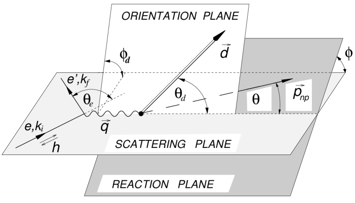
FIG. 1.: Geometry of exclusive electron-deuteron scattering with polarized electrons and an oriented deuteron target. The relative n-p momentum defining with $\vec{q}$ the reaction plane is denoted by $\vec{p}_{np}$ and is characterized by angles $\theta$ and $\phi$. The deuteron orientation axis forming with $\vec{q}$ the orientation plane is denoted by $\vec{d}$ and specified by angles $\theta_{d}$ and $\phi_{d}$.

FIG. 2.: Left: Inclusive form factors $F_{L}$ and $F_{T}$ for $E_{np}=120\,\mbox{MeV}$. Right: Ratio of the form factors with respect to result for $n(r,\chi_{0})\pi\rho_{P}\Delta$ (see Table I). Notation of the curves: dash-dotted: $n(r,\chi_{0})\pi\rho_{P}\Delta$, dashed: $n(r,\chi_{0})\pi(r,t,\chi_{0},\chi_{V})\rho_{P}\Delta$, full: total.

FIG. 3.: Inclusive form factors for a polarized target $F^{20}_{L}$, $F^{20}_{T}$, $F^{2-1}_{LT}$, and $F^{2-2}_{TT}$. Notation of the curves as in Fig. 2.

FIG. 4.: Deuteron electrodisintegration near threshold for $E_{np}=1.5\,\mbox{MeV}$ at backward angles ($\theta_{e}=155^{\circ}$). Left: absolute values; Right: relative with respect to $n\pi\rho_{P}\Delta$. Notation of the curves (see Table I): dotted: $n\pi\rho_{P}\Delta$, dash-dotted: $n(r,\chi_{0})\pi\rho_{P}\Delta$, dashed: $n(r,\chi_{0})\pi(r,t,\chi_{0},\chi_{V})\rho_{P}\Delta$, full: total.

FIG. 5.: Deuteron electrodisintegration near threshold for the “Paris” model of Tamura et al. [8] for $E_{np}=1.5\,\mbox{MeV}$ and $\theta_{e}=155^{\circ}$. Notation of the curves: dotted: $n\pi\Delta$, long-dashed: $n(r,\chi_{0})\pi(r,t,\chi_{0},\chi_{V})\rho(+\omega)_{P}\Delta$, full: total, short-dashed: total result for the OBEPQ-B potential.

FIG. 6.: Deuteron electrodisintegration near threshold: potential model dependence and comparison with experiment. Experimental data points: open triangles: [41], filled circles: [42] ($\theta_{e}=155^{\circ}$, averaged over energies $0\mbox{\,MeV}\leq E_{np}\leq 3\mbox{\,MeV}$; theory for $E_{np}=1.5\mbox{\,MeV}$); filled squares: [43] ($\theta_{e}=180^{\circ}$, averaged over energies $0\mbox{\,MeV}\leq E_{np}\leq 10\mbox{\,MeV}$; theory for $E_{np}=5\mbox{\,MeV}$). Notation of the theoretical curves: full: OBEPQ-B potential, dashed: OBEPQ-A potential, dash-dotted: OBEPQ-C potential.

FIG. 7.: $E_{np}$-$\vec{q}^{\,2}$ plane with indication of the location of the quasi-free ridge and the kinematic sectors, for which the structure functions have been evaluated.

FIG. 8.: The structure functions of the differential cross section for unpolarized electrons and target in the nine kinematic regions of Fig. 7: $f_{L}^{00}$ (top left), $f_{T}^{00}$ (top right), $f_{LT}^{00+}$ (bottom left), and $f_{TT}^{00+}$ (bottom right). Notation of the curves (see Table I): dotted: $n\pi\rho_{P}\Delta$, dash-dotted: $n(r,\chi_{0})\pi\rho_{P}\Delta$, dashed: $n(r,\chi_{0})\pi(r,t,\chi_{0},\chi_{V})\rho_{P}\Delta$, full: total. The top left inset “[$(-n)$ fm]” indicates the unit [$10^{-n}$ fm] for the structure function, and the top right inset “[$E_{np}$/$\vec{q}^{\,2}$]”, where $E_{np}$ in [MeV] and $\vec{q}^{\,2}$ in [fm^-2], indicates the kinematic sector of Fig. 7.

FIG. 9.: As Fig. 8, but for the observable $P_{y}(p)$.

FIG. 10.: The fifth structure function of the differential cross section and the observable $P_{y}(p)$ for longitudinally polarized electrons and an unpolarized target in the nine kinematic sectors of Fig. 7: $f_{LT}^{\prime 00+}$ (left), $f_{LT}^{\prime 00+}(y0)$ (right). Notation of the curves as in Fig. 8.

FIG. 11.: Relativistic contributions from the pionic MEC for unpolarized structure functions. Notation of the curves: dotted: $n(r,\chi_{0})\pi\rho_{P}\Delta$, dash-dotted: $n(r,\chi_{0})\pi(r)\rho_{P}\Delta$, long-dashed: $n(r,\chi_{0})\pi(r,t)\rho_{P}\Delta$, short-dashed: $n(r,\chi_{0})\pi(r,t,\chi_{0})\rho_{P}\Delta$, full: $n(r,\chi_{0})\pi(r,t,\chi_{0},\chi_{V})\rho_{P}\Delta$.

FIG. 12.: As in Fig. 11, for selected polarization structure functions.

FIG. 13.: Effect of the non-Pauli $\rho$-mesonic currents. Notation of the curves: dotted: $n(r,\chi_{0})\pi(r,t,\chi_{0},\chi_{V})\Delta$, dash-dotted: $n(r,\chi_{0})\pi(r,t,\chi_{0},\chi_{V})\rho_{P}\Delta$, full: $n(r,\chi_{0})\pi(r,t,\chi_{0},\chi_{V})\rho(\chi_{0})\Delta$.

FIG. 14.: Effect of the heavy meson exchange currents (the contributions of $\eta$, $\omega$, $\sigma$, and $\delta$ are summed up). Notation of the curves: dotted: $n(r,\chi_{0})\pi(r,t,\chi_{0},\chi_{V})\rho\Delta$, dash-dotted: $n(r,\chi_{0})\pi(r,t,\chi_{0},\chi_{V})\rho(\chi_{0})h(\chi_{0})\Delta$, full: total.

FIG. 15.: The neutron polarization $P^{\prime}_{x}(n)$ and the vector beam-target asymmetry $A^{V}_{ed}$ for the kinematics $E_{np}=120\,\mbox{MeV}$, $\vec{q}^{\,2}=12\,\mbox{fm}^{-2}$. Notation of the curves: dash-dotted: $n(r,\chi_{0})\pi\rho_{P}\Delta$, dashed: $n(r,\chi_{0})\pi(r,t,\chi_{0},\chi_{V})\rho_{P}\Delta$, full: total.

REFERENCES

• [1] A. Cambi, B. Mosconi, and P. Ricci, Phys. Rev. Lett. 48, 462 (1982).
• [2] M. van der Schaar et al., Phys. Rev. Lett. 68, 776 (1992).
• [3] B.D. Keister and W.N. Polyzou, Adv. Nucl. Phys. 20, 225 (1991).
• [4] N.K. Devine and S.J. Wallace, Phys. Rev. C 48, R973 (1993).
• [5] J. Tjon, Proc. 14th Int. Conf. on Few Body Problems, Williamsburg, 1994, ed. F. Gross, AIP Conf. Proc. 334, 177 (1995).
• [6] Various methods are discussed and a number of useful references is given in:
J.L. Friar, Phys. Rev. C 22, 796 (1980);
J. Adam, Jr., Proc. 14th Int. Conf. on Few Body Problems, Williamsburg, 1994, ed. F. Gross, AIP Conf. Proc. 334, 192 (1995).
• [7] E. Truhlik and J. Adam, Jr., Nucl. Phys. A492, 529 (1989).
• [8] K. Tamura, T. Niwa, T. Sato, and H. Ohtsubo, Nucl. Phys. A536, 597 (1992).
• [9] H. Göller and H. Arenhövel, Few-Body Syst. 13, 117 (1992).
• [10] J. Adam, Jr., E. Truhlik, and D. Adamova, Nucl. Phys. A492, 556 (1989).
• [11] N. Fukuda, K. Sawada, and M. Taketani, Progr. Theor. Phys. 12, 156 (1954).
• [12] J.D. Bjorken and S.D. Drell, Relativistic Quantum Mechanics (McGraw-Hill, New York, 1964).
• [13] F.J. Dyson, Phys. Rev. 73, 929 (1948).
• [14] M.V. Barnhill III, Nucl. Phys. A131, 106 (1969).
• [15] J. Adam, Jr., H. Göller, and H. Arenhövel, Phys. Rev. C 48, 370 (1993).
• [16] R. Machleidt, K. Holinde, and Ch. Elster, Phys. Rep. 149, 1 (1987).
• [17] R. Machleidt, Adv. Nucl. Phys. 19, 189 (1989).
• [18] R.A. Krajcik and L.L. Foldy, Phys. Rev. D 10, 1777 (1974).
• [19] J.L. Friar, Ann. of Phys. 104 (NY), 380 (1977).
• [20] J.L. Friar, in Mesons in Nuclei, eds. M. Rho and D.H. Wilkinson, vol. II (North-Holland Publishing Company, Amsterdam, 1979) p. 595.
• [21] W. Leidemann and H. Arenhövel, Nucl. Phys.  A465, 573 (1987).
• [22] P. Wilhelm and H. Arenhövel, Phys. Lett. B318, 410 (1993).
• [23] H. Arenhövel, W. Leidemann, and E.L. Tomusiak, Few-Body Syst. 15, 109 (1993).
• [24] H. Arenhövel and K.-M. Schmitt, Few-Body Syst. 8, 77 (1990).
• [25] H. Arenhövel, W. Leidemann, and E.L. Tomusiak, Phys. Rev. C 46, 455 (1992).
• [26] T. Wilbois, G. Beck, and H. Arenhövel, Few-Body Syst. 15, 39 (1993).
• [27] H. Arenhövel, W. Leidemann, and E.L. Tomusiak, Phys. Rev. C 52, 1232 (1995).
• [28] W. Fabian and H. Arenhövel, Nucl. Phys. A314, 253 (1979).
• [29] S. Galster, H. Klein, J. Moritz, K.H. Schmidt, D. Wegener, and J. Bleckwenn, Nucl. Phys. B32, 221 (1971).
• [30] H. Pöpping, P.U. Sauer, and X. Zhang, Nucl. Phys. A474, 557 (1987);
H. Pöpping, P.U. Sauer, and X. Zhang, Nucl. Phys. A550, 563 (1992).
• [31] T. Wilbois, PhD Thesis, Mainz 1996 (unpublished).
• [32] R.M. Davidson, N.C. Mukhopadhyay, and R.S. Wittman, Phys. Rev. D 43, 71 (1991).
• [33] J. Hockert, D.O. Riska, M. Gari, and A. Huffman, Nucl. Phys. A217, 14 (1973).
• [34] J.A. Lock and L.L. Foldy, Ann. of Phys. 93, 276 (1975).
• [35] W. Fabian and H. Arenhövel, Nucl. Phys. A258, 461 (1976).
• [36] B. Mosconi and P. Ricci, Nuov. Cim. 36A, 67 (1976).
• [37] W. Leidemann and H. Arenhövel, Nucl. Phys. A393, 385 (1983).
• [38] S.K. Singh, W. Leidemann, and H. Arenhövel, Z. Phys. A331, 509 (1988).
• [39] E. Hummel, PhD Thesis, Utrecht 1991 (unpublished).
• [40] W. Leidemann, K.-M. Schmitt, and H. Arenhövel, Phys. Rev. C 42, R826 (1990).
• [41] M. Bernheim, E. Jans, J. Mougey, D. Royer, D. Tarnowski, S. Turck-Chieze, I. Sick, G.P. Capitani, E. De Sanctis, and S. Frullani, Phys. Rev. Lett. 46, 402 (1981).
• [42] S. Auffret et al., Phys. Rev. Lett. 55, 1362 (1985).
• [43] R.G. Arnold et al., Phys. Rev. C 42, R1 (1990).
• [44] R. Schiavilla and D.O. Riska, Phys. Rev. C 43, 437 (1991).
• [45] A.J.F. Siegert, Phys. Rev. 52, 787 (1937).
• [46] T. Eden et al., Phys. Rev. C 50, R1749 (1994).
• [47] M. Meyerhoff et al., Phys. Lett. B327, 201 (1994).
• [48] F. Klein for the A3-collaboration at MAMI, Proc. PANIC 96, Williamsburg, 1996 (in print).
• [49] B. Mosconi, J. Pauschenwein, and P. Ricci, Phys. Rev. C 48, 332 (1993).
• [50] R.W. Wiringa, R. Smith, and T.L. Ainsworth, Phys. Rev. C 29, 1207 (1984).
• [51] D.O. Riska, Phys. Rep. 181, 207 (1989).