Electromagnetic Production of the Hypertriton

Abstract

Kaon photoproduction on ³He, $\gamma~{}+~{}^{3}{\mathrm{H}e}\longrightarrow K^{+}+~{}^{3}_{\Lambda}{\mathrm{H}}$, is studied in the framework of the impulse approximation. Realistic ³He wave functions obtained as solutions of Faddeev equations with the Reid soft-core potential are used along with different ${}^{3}_{\Lambda}$H wave functions. Results are compared for several elementary operator models, which can successfully describe the elementary kaon production off the proton up to a photon lab energy of $k=2.2$ GeV. It is found that the corresponding cross sections are small, of the order of several nanobarns. It is also shown that the influence of Fermi motion is important, while the effect of different off-shell assumptions on the cross section is not too significant.
PACS number(s) : 13.60.Le, 25.20.Lj, 21.80.+a
Keywords : Kaon photoproduction, Hypertriton, Impulse approximation

I INTRODUCTION

With the start of experimental activities at Jefferson Lab, the electromagnetic production of hypernuclei will become experimentally feasible. This reaction offers a particularly efficient tool to study the production and interactions of hyperons in the nuclear medium. The reaction is of special interest in the case of the lightest hypernucleus, the hypertriton ${}^{3}_{\Lambda}$H. Studies of the hypertriton can provide relevant new information on the $YN$ interaction, which up to now is only poorly known from the available $YN$ scattering data. Furthermore, with the hypertriton being the lightest hypernucleus, it is obviously the first system in which the $YN$ potential, including the interesting $\Lambda$-$\Sigma$ conversion potential, can be tested in the nuclear environment. This is also supported by the fact that neither the $\Lambda N$ nor the $\Sigma N$ interactions are sufficiently strong to produce a bound two-body system. Therefore the hypertriton will play an important role in hypernuclear physics, similar to the deuteron in nuclear physics.

Recently, the Bochum Group [1] has investigated the hypertriton using the Jülich hyperon-nucleon potential in the one-boson-exchange (OBE) parametrization (model $\tilde{\mathrm{A}}$ of Ref. [2]) combined with various realistic $NN$ interactions. They found that with this potential the hypertriton turns out to be unbound. Only an increase by about 4% in the Jülich potential (multiplication of the ${}^{1}S_{0}~{}YN$ partial wave by a factor of 1.04) leads to a bound state for the hypertriton. On the other hand, the use of the Nijmegen hyperon-nucleon potential [3] in the same calculation [4] leads to a bound hypertriton. Clearly, significant improvement is still needed in the hyperon-nucleon force sector, where in contrast to the nucleon-nucleon sector the dominant one-pion-exchange (OPE) tensor force is not present since the lambda ($I=0$) and the nucleon ($I=\frac{1}{2}$) cannot exchange a pion ($I=1$).

Hypernuclear systems have been extensively studied experimentally for a wide range of nuclei (from ${}^{3}_{\Lambda}$H to ${}^{208}_{~{}~{}\Lambda}{\mathrm{P}b}$ [5]) by employing hadronic processes such as stopped and low momentum kaon induced reactions, ${\mathrm{A}}(K,\pi)_{\Lambda}{\mathrm{B}}$, as well as ${\mathrm{A}}(\pi,K)_{\Lambda}{\mathrm{B}}$ reactions (see Ref. [6] for a recent review of hypernuclear physics). Nevertheless, since the different mechanisms are complementary, electromagnetic productions will, at some point, be required for a complete understanding of hypernuclear spectra.

Several theoretical studies of hypernuclear electromagnetic productions have been performed during the last few years [7, 8]. The reactions ${}^{40}{\mathrm{C}a}(\gamma,K^{+})^{40}_{~{}\Lambda}{\mathrm{K}}$ and ${}^{208}{\mathrm{P}b}(\gamma,K^{+})^{208}_{~{}~{}\Lambda}{\mathrm{T}l}$, for instance, have been calculated within the framework of a distorted wave impulse approximation (DWIA), where the interaction of the kaon with the final state has been included via a rather weak optical potential derived from the elementary $KN$ amplitudes. In contrast to the elementary processes, where both $S=J=0$ and $S=J=1$ transition terms contribute equally to the cross section, the production from nuclei can eliminate $S=0$ or $S=1$ contributions in certain transitions. The production of $\Sigma$ hypernuclei in reactions such as ${}^{16}{\mathrm{O}}(\gamma,K^{+})^{16}_{~{}\Sigma}{\mathrm{N}}$, ${}^{40}{\mathrm{C}a}(\gamma,K^{+})^{40}_{~{}\Sigma}{\mathrm{K}}$, and ${}^{208}{\mathrm{P}b}(\gamma,K^{+})^{208}_{~{}~{}\Sigma}{\mathrm{T}l}$ [8] has also been calculated.

In this work we consider the reaction ${}^{3}{\mathrm{H}e}(\gamma,K^{+})^{3}_{\Lambda}{\mathrm{H}}$, i.e. the incoming real photon interacts with a nucleon (proton) in ³He creating a lambda which combines with the other two nucleons to form the bound hypertriton and a positively charged kaon which exits the nucleus. To our knowledge, no analysis has been made and no experimental data are available for this reaction. A recent calculation of Komarov et al. [9], who studied the proton-nucleus collision

$$p+d\longrightarrow K^{+}+~{}^{3}_{\Lambda}{\mathrm{H}}$$ (1)

estimated that at an incident proton energy $T_{p}$ = 1.13 - 3.0 GeV, the maximum differential cross section is well below 1 nb/sr, making experimental verification very difficult. It has been pointed out that this result is 50 times smaller than in the case of eta production through $p$-$d$ collisions.

On the other hand, Tiator et al. [10] have estimated the differential cross section of eta photoproduction on ³He at $k=750$ MeV, close to threshold, to be around 100 nb/sr at $\theta_{\mathrm{c}.m.}=0^{\circ}$, with an expected decrease to 1 nb/sr at $\theta_{\mathrm{c}.m.}=60^{\circ}$. Since the cross section of elementary eta production is approximately 10 times larger than for the kaon, one would not expect a cross section larger than 10 nb/sr for kaon production on ³He.

In this study we will evaluate the elementary operator for kaon photoproduction between a realistic wave function of ³He, obtained as a solution of the Faddeev equations with the Reid soft core potential [11], and the simple hypertriton wave function developed in Ref. [12]. This simple hypertriton model used in our calculation [12] has been adjusted to reproduce the experimental $\Lambda$-$d$ binding energy (0.13 $\pm$ 0.05 MeV) [13], and it predicts the branching ratio [14]

$$R = \frac{\Gamma(~{}^{3}_{\Lambda}{\mathrm{H}}\rightarrow\pi^{-}+~{}^{3}{\mathrm{H}e}~{})}{\Gamma(~{}^{3}_{\Lambda}{\mathrm{H}}\rightarrow\pi^{-}+{\mathrm{a}ll}~{})}~{}=~{}0.35\pm 0.04~{}.$$ (2)

While we use this simple wave function for most calculations we also perform comparisons with the correlated Faddeev wave function of Ref. [4] in order to assess the sensitivity of the cross section predictions to different hypertriton descriptions.

In section II, we briefly review the three-body wave functions used in our calculation along with some experimental facts on both ³He and the hypertriton. Section III explains the matrix elements of the process. The present status of elementary models used in our calculation is briefly reviewed in section IV. The results of our investigation are presented and discussed in section V. We summarize our findings in section VI.

II THE THREE-BODY WAVE FUNCTIONS

Since both ³He and the hypertriton are three-body systems, we will describe the reaction using familiar three-body coordinates. In the Jacobi representation, the three-body momentum coordinates for particles with momenta ${\vec{k}}_{1}$, ${\vec{k}}_{2}$, and ${\vec{k}}_{3}$, and masses $m_{1}$, $m_{2}$, and $m_{3}$, respectively, are given by

$${\vec{P}}~{}=~{}{\vec{k}}_{1}+{\vec{k}}_{2}+{\vec{k}}_{3}~{}~{},~{}~{}{\vec{p}}~{}=~{}\frac{m_{3}{\vec{k}}_{2}-m_{2}{\vec{k}}_{3}}{m_{2}+m_{3}}~{}~{},~{}~{}{\vec{q}}~{}=~{}\frac{(m_{2}+m_{3}){\vec{k}}_{1}-m_{1}({\vec{k}}_{2}+{\vec{k}}_{3})}{m_{1}+m_{2}+m_{3}}~{}.$$ (3)

For the case of ³He, all constituents are assumed to have the same masses, and Eq. (3), in the center of momentum of the particles, reduces to

$${\vec{P}}~{}=~{}{\vec{0}}~{}~{}~{},~{}~{}~{}{\vec{p}}~{}=~{}{\textstyle\frac{1}{2}}\,({\vec{k}}_{2}-{\vec{k}}_{3})~{}~{}~{},~{}~{}~{}{\vec{q}}~{}=~{}{\vec{k}}_{1}~{}.$$ (4)

However, in the case of the hypertriton, the hyperon is clearly heavier than the proton or the neutron. Nevertheless, if we assume that the hyperon is particle 1, Eq. (3) may still be reduced to Eq. (4).

In Lovelace coordinates, the expression corresponding to Eq. (4) is given by

$${\vec{P}}~{}=~{}{\vec{0}}~{}~{}~{},~{}~{}~{}{\vec{p}}~{}=~{}{\textstyle\frac{1}{2}}\,({\vec{k}}_{2}-{\vec{k}}_{3})~{}~{}~{},~{}~{}~{}{\vec{q}}~{}=~{}-{\textstyle\frac{1}{2}}\sqrt{3}\,{\vec{k}}_{1}~{}.$$ (5)

Hence, the two coordinate systems differ only in the spectator coordinate by a factor of $-\frac{1}{2}\sqrt{3}$. Using the latter coordinate system we will express the nuclear matrix element $T_{\mathrm{f}i}$ of the reaction in the lab frame as

$$T_{\mathrm{f}i} = \langle~{}^{3}_{\Lambda}{\mathrm{H}}~{}|~{}t^{\gamma p\rightarrow K^{+}\Lambda}~{}|~{}^{3}{\mathrm{H}e}~{}\rangle~{},$$ (6)

where the production operator, $t^{\gamma p\rightarrow K^{+}\Lambda}$, is obtained from the elementary reaction.

A The ³He Wave Function

In our formalism, the three-body wave functions are expanded in orbital momentum, spin, and isospin of the pair (2,3) and the spectator (1) with the notation

$$\Psi_{{}^{3}{\mathrm{H}e}}({\vec{p}},{\vec{q}}\,) = \sum_{\alpha}\phi_{\alpha}(p,q)~{}|(Ll){\cal L},(S{\textstyle\frac{1}{2}}){\cal S},{\textstyle\frac{1}{2}}M\rangle~{}|(T{\textstyle\frac{1}{2}}){\textstyle\frac{1}{2}}M_{t}\rangle~{},$$ (7)

where $\phi_{\alpha}(p,q)$ stands for numerical solutions of Faddeev equations using the realistic nucleon-nucleon potential [11].

In Eq. (7) we have introduced $\alpha=\{Ll{\cal L}S{\cal S}T\}$ to shorten the notation, where $L$, $S$, and $T$ are the total angular momentum, spin, and isospin of the pair (2,3), while for the spectator (1) the corresponding observables are labelled by $l$, $\frac{1}{2}$, and $\frac{1}{2}$, respectively. From now on we will use the Lovelace coordinates for the momenta of the pair and of the spectator. Their quantum numbers, along with the probabilities for the 11 partial waves, are listed in Table I. Clearly, most contributions will come from the first two partial waves (with a total probability of 88%), which represent the $S$-waves with isospin 0 and 1, respectively.

B The Hypertriton

The term “hypertriton” commonly refers to the bound state consisting of a proton, a neutron, and a lambda hyperon. Although a hypertriton consisting of a proton, a neutron, and a $\Sigma$ hyperon could exist, no experimental information is available at present [15]. The existing experimental information on the hypertriton is mostly from old bubble-chamber measurements [16]. Table II compares its properties with the triton and the deuteron.

Many models of the hypertriton have been developed using Faddeev equations [1, 4, 17], the resonating group method [18], variational methods [19], and hyperspherical harmonics [20]. We choose the simple model developed in Ref. [12], which should be reliable enough to obtain a first estimate for the photoproduction of the hypertriton.

In this model, the hypertriton is described by a deuteron and a lambda moving in an effective $\Lambda$-$d$ potential. The influence of the lambda on the two nucleons is neglected, thus the nucleon part of the wave functions is exactly that of a free deuteron. We have also neglected the $\Lambda N\rightarrow\Sigma N$ conversion, because the $\Sigma NN$ component in the hypertriton wave functions has been calculated to be very small. Using the phenomenological $YN$ potential developed in Ref. [21], the authors of Ref. [22] found a probability of only $0.36\%$ to have a $\Sigma NN$ component in the hypertriton. This has been recently confirmed by the Bochum group. Using the Nijmegen $YN$ potential [3] and the Nijmegen93 $NN$ potential [23] they obtained a probability of $0.5\%$ [4]. For other realistic $NN$ potentials the results are in the same range.

The effective $\Lambda$-$d$ potential is constructed as follows: First, a separable fit is performed to the $\Lambda N$ $S$-wave interaction given by the Nijmegen $YN$ soft-core potential [3], which is then spin averaged over the $\Lambda N$ configurations found in the hypertriton. The $\Lambda N$ potential is summed over the two nucleons and averaged over the deuteron wave function. Finally, the resulting $\Lambda$-$d$ potential is fitted to a separable form, retaining only the $S$-wave part. The $\Lambda$-$d$ binding energy can then be reproduced by some fine tuning of the $\Lambda$-$d$ potential parameters.

With the notation of Eq. (4), the hypertriton wave function may be written as

$$\Psi_{{}^{3}_{\Lambda}{\mathrm{H}}}({\vec{p}},{\vec{q}}\,) = \sum_{\alpha}\phi_{\alpha}(p,q)~{}|(Ll){\cal L},(S{\textstyle\frac{1}{2}}){\cal S},{\textstyle\frac{1}{2}}M\rangle~{},$$ (8)

where $\phi_{\alpha}(p,q)$ is now simply given by the two separable wave functions of the deuteron and the lambda,

$$\phi_{\alpha}(p,q) = \Psi^{(L)}_{d}(p)~{}\varphi_{\Lambda}(q)~{}.$$ (9)

In Eq. (8), we have dropped the isospin part of the wave function since the hypertriton has isospin 0. This argument is based on the fact that only the $\Lambda np$ system appears to exist in nature, and that $\Lambda nn$ and $\Lambda pp$ bound systems have never been observed. Furthermore, it has been shown in Ref. [4] that the states of the $\Lambda(\Sigma)NN$ system with quantum numbers $(T,J)$ different from $(0,\frac{1}{2})$ are not bound. Only the quantum numbers $\alpha=\{0001\frac{1}{2}0\}$ and $\{2021\frac{3}{2}0\}$ are non-zero in Eq. (8). The probabilities for both partial waves are shown in the last column of Table I, where we have used the Paris potential for the deuteron part. It is clear that the two probabilities originate only from the deuteron, since the lambda part does not depend upon any of the quantum numbers.

The lambda part of the wave functions is found by solving the Schrödinger equation for a particle moving in the $\Lambda$-$d$ effective potential. The solution is assumed to have the form

$$\varphi_{\Lambda}(q) = N(Q_{\Lambda})~{}\frac{\exp[-(q/Q_{\Lambda})^{2}]}{q^{2}+\alpha^{2}}~{},$$ (10)

with $\alpha=(6.8\pm 1.3)\times 10^{-2}~{}{\mathrm{f}m}^{-1}$, proportional to the square-root of the lambda binding energy, and the normalization factor

$$N(Q_{\Lambda}) = \left[~{}\frac{\pi}{4\alpha}~{}\left\{{\mathrm{c}erfe}\left(\frac{\sqrt{2}\alpha}{Q_{\Lambda}}\right)\left(1+\frac{4\alpha^{2}}{Q_{\Lambda}^{2}}\right)-\frac{2\alpha}{Q_{\Lambda}}\left(\frac{2}{\pi}\right)^{\frac{1}{2}}\right\}~{}\right]^{-\frac{1}{2}}~{},$$ (11)

where

$${\mathrm{c}erfe}(x)~{}=~{}{\mathrm{e}xp}(x^{2})\left[1-{\mathrm{e}rf}(x)\right]~{}~{}~{},~{}~{}~{}{\mathrm{e}rf}(x)~{}=~{}\frac{2}{\sqrt{\pi}}\int_{0}^{x}{\mathrm{e}xp}(-t^{2})~{}dt~{}.$$ (12)

The author of Ref. [12] used the $\Lambda$-$d$ potential range $Q_{\Lambda}=1.17~{}{\mathrm{f}m}^{-1}~{}(\sim\pm 10\%)$, leading to $[N(1.17)]^{2}=0.1039$. From Eq. (10) it is obvious that the lambda part of the hypertriton wave functions drops drastically as function of the momentum $q$. It is also apparent that the most probable momenta of the lambda particle in the hypertriton are in the vicinity of 0.1 fm^-1.

III THE MATRIX ELEMENTS

Following the investigations of coherent pion photoproduction on ³He by Tiator et al. [28, 29, 30], we calculate the reaction in momentum space. The Feynman diagram for photoproduction of the hypertriton is depicted in Fig. 1, and the most important contributions to this process are shown in Fig. 2. For our present purpose, we will only consider the first diagram, corresponding to the impulse approximation, i.e. the photon only interacts with one nucleon, while the other two nucleons of ³He act as spectators. We also neglect the final state interaction (FSI) of the $K^{+}$ with the hypertriton. For ${}^{12}{\mathrm{C}}(\gamma,K^{+})^{12}_{~{}\Lambda}{\mathrm{B}}$, the $K^{+}$ FSI was found to reduce the cross sections by 30% [8], thus one would not expect FSI to affect our results by more than 5–10%.

In the case of kaon photoproduction on the nucleus, the cross section in the lab system can be written as

$$\frac{d\sigma_{\mathrm{T}}}{d\Omega_{K}} = \frac{|{\vec{q}}_{K}^{\mathrm{~{}}c.m.}|}{|{\vec{k}}^{\mathrm{c}.m.}|}~{}\frac{M_{\mathrm{}3He}E_{\mathrm{}3_{\Lambda}H}}{64\pi^{2}W^{2}}~{}\sum_{\epsilon}\sum_{M,M^{\prime}}~{}\left|T_{\mathrm{f}i}\right|^{2}~{},$$ (13)

where the sums are over the photon polarization and over the initial and final spin projections of the nucleus.

The transition matrix elements can be expressed in terms of an integral over all internal momenta and states contributing to the process [28, 29],

$$T_{\mathrm{f}i} = \sqrt{3}\int d^{3}{\vec{p}}~{}d^{3}{\vec{q}}\Psi_{\mathrm{}{3}_{\Lambda}H}({\vec{p}},{\vec{q}}\,^{\prime})~{}t^{\gamma p\rightarrow K\Lambda}({\vec{q}},{\vec{Q}})~{}\Psi_{\mathrm{}{3}He}({\vec{p}},{\vec{q}}\,)$$ (14)

$$= 2\sqrt{6}~{}\sum_{\left.\begin{array}[]{c}\alpha(Ll{\cal L}S{\cal S})\\ \alpha^{\prime}(L^{\prime}l^{\prime}{\cal L}^{\prime}S^{\prime}{\cal S}^{\prime})\\ n\lambda\Lambda m_{\Lambda}\end{array}\right.}~{}\Biggl{[}~{}i^{n}~{}\hat{n}\hat{\cal L}^{\prime}\hat{\cal L}\hat{\cal S}^{\prime}\hat{\cal S}\hat{\lambda}\hat{\Lambda}~{}(-1)^{n+l^{\prime}+l+L+S+{\cal L}+{\cal S}+M}~{}\delta_{LL^{\prime}}~{}\delta_{SS^{\prime}}~{}\delta_{T0}\times$$ (28)

$$\left(\begin{array}[]{rrr}\frac{1}{2}&\frac{1}{2}&\Lambda\\ M^{\prime}&-M&m_{\Lambda}\end{array}\right)\left\{\begin{array}[]{lll}{\cal L}&{\cal L}^{\prime}&\lambda\\ l^{\prime}&l&L\end{array}\right\}\left\{\begin{array}[]{lll}{\cal S}^{\prime}&{\cal S}&n\\ \frac{1}{2}&\frac{1}{2}&S\end{array}\right\}\left\{\begin{array}[]{lll}{\cal L}&{\cal S}&\frac{1}{2}\\ {\cal L}^{\prime}&{\cal S}^{\prime}&\frac{1}{2}\\ \lambda&n&\Lambda\end{array}\right\}~{}I^{\alpha\alpha^{\prime}}_{\lambda n\Lambda m_{\Lambda}}({\vec{q}},{\vec{q}}\,^{\prime})~{},$$

with the four-dimensional integrals

$$I^{\alpha\alpha^{\prime}}_{\lambda n\Lambda m_{\Lambda}}({\vec{q}},{\vec{q}}\,^{\prime}) = \int d^{3}{\vec{q}}~{}p^{2}dp~{}\phi_{\alpha^{\prime}}(p,q\,^{\prime})~{}\phi_{\alpha}(p,q)~{}\times$$ (30)

$$\Bigl{[}\Bigl{[}{\bf Y}^{(l^{\prime})}(\hat{{\vec{q}}\,^{\prime}})\otimes{\bf Y}^{(l)}(\hat{{\vec{q}}\,})\Bigr{]}^{(\lambda)}\otimes{\bf K}^{(n)}\Bigr{]}^{(\Lambda)}_{m_{\Lambda}}~{}$$

to be evaluated numerically. The factor of $\sqrt{3}$ on the right hand side of Eq. (28) comes from the antisymmetry of the initial state. For the simple case of only $S$-state wave functions ($L^{\prime}=l^{\prime}={\cal L}^{\prime}=0$, $S^{\prime}=1$, ${\cal S}^{\prime}=\frac{1}{2}$), Eq. (28) reduces to

$$T_{\mathrm{f}i} = \sqrt{\frac{6}{\pi}}~{}\sum_{\alpha{\alpha}^{\prime}}~{}\sum_{n\Lambda m_{\Lambda}}i^{n}\hat{n}\hat{{\cal L}}\hat{{\cal S}}\hat{{\cal S}^{\prime}}\hat{\Lambda}(-)^{1+n+{{\cal S}}+M}\delta_{SS^{\prime}}\delta_{LL^{\prime}}\delta_{T0}\times$$ (40)

$$\left(\begin{array}[]{ccc}\frac{1}{2}&\frac{1}{2}&\Lambda\\ M^{\prime}&-M&m_{\Lambda}\end{array}\right)\left\{\begin{array}[]{ccc}{{\cal S}}&{{\cal S}^{\prime}}&n\\ \frac{1}{2}&\frac{1}{2}&1\end{array}\right\}\left\{\begin{array}[]{ccc}{{\cal L}}&{{\cal S}}&\frac{1}{2}\\ L&{{\cal S}^{\prime}}&\frac{1}{2}\\ l&n&\Lambda\end{array}\right\}\times$$

$$\int d^{3}{\vec{q}}~{}p^{2}dp~{}\varphi_{\Lambda}(q\,^{\prime})~{}\Psi_{d}^{(L)}(p)~{}\phi_{\alpha}(p,q)~{}\left[{\bf Y}^{(l)}(\hat{{\vec{q}}\,})\otimes{\bf K}^{(n)}\right]^{(\Lambda)}_{m_{\Lambda}}~{},$$

In Eqs. (28) and (40) we have used the Lovelace coordinate for the produced hyperon

$${\vec{q}}\,^{\prime}={\vec{q}}-\frac{1}{\sqrt{3}}{\vec{Q}}~{},$$ (41)

where ${\vec{Q}}$ is the momentum transfer to the nucleus,

$${\vec{Q}}={\vec{k}}-{\vec{q}}_{K}~{}.$$ (42)

Finally, the elementary production operator in Eq. (6), involving an invariant product between the photon polarization $\epsilon_{\mu}$ and the electromagnetic current $J_{\mu}$, has been decomposed into spin-independent and spin-dependent amplitudes

$$t^{\gamma p\rightarrow K^{+}\Lambda} = \epsilon_{\mu}~{}J^{\mu}$$ (43)

$$= L+i{\vec{\sigma}}\cdot{\vec{K}}$$ (44)

$$= \sum_{n=0,1}(-i)^{n~{}}\hat{n}~{}\left[{\mbox{\boldmath{$\sigma$}}}^{(n)}\otimes{\bf K}^{(n)}\right]^{(0)}~{},$$ (45)

with $\hat{n}=\sqrt{2n+1}$, ${\mbox{\boldmath{$\sigma$}}}^{(0)}=1$, and ${\bf K}^{(0)}=L$. The elementary production amplitudes $L$ and ${\vec{K}}$ are calculated from the non-relativistic reduction of the elementary operator (see Appendix A) and are given by

$$L = N~{}\biggl{\{}-{\cal{F}}_{14}~{}{\vec{p}}_{p}+{\cal{F}}_{15}~{}({\vec{q}}_{K}-{\vec{p}}_{p})\biggr{\}}\cdot({\vec{k}}\times{\vec{\epsilon}}\,)$$ (46)

$${\vec{K}} = -N~{}\biggl{[}~{}\biggl{\{}{\cal{F}}_{1}+({\cal{F}}_{14}-{\cal{F}}_{15})~{}{\vec{k}}~{}\cdot{\vec{p}}_{p}-{\cal{F}}_{15}~{}(|{\vec{k}}|^{2}-{\vec{k}}\cdot{\vec{q}}_{K})\biggr{\}}~{}{\vec{\epsilon}}$$ (50)

$$+~{}\biggl{\{}({\cal{F}}_{4}+{\cal{F}}_{5}+{\cal{F}}_{12}+{\cal{F}}_{13}-{\cal{F}}_{14}+{\cal{F}}_{15})~{}{\vec{p}}_{p}\cdot{\vec{\epsilon}}-({\cal{F}}_{5}+{\cal{F}}_{13}+{\cal{F}}_{15})~{}{\vec{q}}_{K}\cdot{\vec{\epsilon}}~{}\biggr{\}}~{}{\vec{k}}$$

$$+~{}\biggl{\{}({\cal{F}}_{8}+{\cal{F}}_{9}+{\cal{F}}_{12}+{\cal{F}}_{13})~{}{\vec{p}}_{p}\cdot{\vec{\epsilon}}-({\cal{F}}_{9}+{\cal{F}}_{13})~{}{\vec{q}}_{K}\cdot{\vec{\epsilon}}~{}\biggr{\}}~{}{\vec{p}}_{p}$$

$$+~{}\biggl{\{}-({\cal{F}}_{12}+{\cal{F}}_{13})~{}{\vec{p}}_{p}\cdot{\vec{\epsilon}}+{\cal{F}}_{13}~{}{\vec{q}}_{K}\cdot{\vec{\epsilon}}~{}\biggr{\}}~{}{\vec{q}}_{K}~{}\biggr{]}~{},$$

where we have neglected small terms ${\cal F}_{16}$ - ${\cal F}_{20}$ in our non-relativistic approximation, and dropped all terms containing $k^{2}$, ${\vec{k}}\cdot{\vec{\epsilon}}$, and $\epsilon_{0}$, since these terms will not contribute to photoproduction. It is easy to show that the omission of ${\cal F}_{16}$ - ${\cal F}_{20}$ will not destroy gauge invariance of the transition matrix. The analytical expressions of ${\cal F}_{1}$ - ${\cal F}_{20}$ and $N$ are given in Appendix A.

The tensor operators, $\left[{\bf Y}^{(l)}(\hat{{\vec{q}}\,})\otimes{\bf K}^{(n)}\right]^{(\Lambda)}_{m_{\Lambda}}$, which determine the specific nuclear transitions in the reaction, are given in Table III. In contrast to Ref. [28], the tensor operators in our case are simplified by the approximation that the hypertriton wave function only contains the partial wave with $l^{\prime}=0$. However, for future studies involving more advanced hypertriton wave functions [1, 4], the complete operator will be needed. For this purpose, we have also derived the form of Eq. (40) for the more general case [31].

Since both initial and final states of the nucleus are unpolarized, the sums over the spin projections can be performed by means of

$$\sum_{M,M^{\prime}}~{}\left|T_{\mathrm{f}i}\right|^{2} = \sum_{\Lambda,m_{\Lambda}}~{}\left|T^{(\Lambda)}_{m_{\Lambda}}\right|^{2}~{},$$ (51)

with

$$T^{(\Lambda)}_{m_{\Lambda}} = \sqrt{\frac{6}{\pi}}~{}\sum_{\alpha,{\alpha}^{\prime},n}\left[~{}i^{n}~{}\hat{n}\hat{\cal L}\hat{S}^{\prime}\hat{S}(-1)^{n+{\cal S}-\frac{1}{2}}\left\{\begin{array}[]{lll}{\cal S}^{\prime}&{\cal S}&n\\ \frac{1}{2}&\frac{1}{2}&1\end{array}\right\}\left\{\begin{array}[]{lll}{\cal L}&{\cal S}&\frac{1}{2}\\ L&{\cal S}^{\prime}&\frac{1}{2}\\ l&n&\Lambda\end{array}\right\}\delta_{LL^{\prime}}\delta_{S1}\delta_{T0}~{}\times\right.$$ (58)

$$\int d^{3}{\vec{q}}~{}p^{2}dp~{}\varphi_{\Lambda}(q\,^{\prime})~{}\Psi_{d}^{(L)}(p)~{}\phi_{\alpha}(p,q)~{}\Bigl{[}{\bf Y}^{(l)}(\hat{{\vec{q}}\,})\otimes{\bf K}^{(n)}\Bigr{]}^{(\Lambda)}_{m_{\Lambda}}\Biggr{]}.~{}$$

Since the tensor ${\bf K}^{(n)}$ contains complicated functions of the integration variables ${\vec{q}}$ and $\hat{{\vec{q}}\,}=\Omega_{q}$, the integral in Eq. (58) has to be performed numerically. It is appropriate to perform the overlap integration in $p$ first, because in the impulse approximation the tensor operator does not depend on the relative pair momentum.

IV Elementary Models

Most current elementary models were developed to fit experimental data below 1.5 GeV. In recent analyses, only Refs. [32, 33] and the model of Ref. [31] fit the photo- and electroproduction data up to 2.2 GeV. The recent analysis of Ref. [32] gives a very comprehensive description of the elementary process. However, since this model incorporates spin 5/2 resonances, the corresponding elementary operator is rather cumbersome for nuclear applications. Therefore, we will not include this model in our calculations. In Table IV we present the coupling constants for different models of the elementary reaction. We note that present elementary models suffer from several fundamental uncertainties, such as the number of resonances to be included in view of the relatively high production threshold. For the sake of simplicity, current models usually incorporate only few of them. Other complications arise from the extracted leading coupling constants, which are difficult to reconcile with the SU(3) predictions.

The elementary model developed in Ref. [31] incorporates the intermediate $K^{*}$-exchange, the $N^{*}$ resonances $S_{11}$(1650) and $P_{11}$(1710) and, in addition, the $s$-channel $\Delta$ resonances $S_{31}$(1900) and $P_{31}$(1910) for $K\Sigma$ photoproduction. To achieve a reasonable $\chi^{2}$ for the experimental data in all six isospin channels, Ref. [31] introduced a hadronic form factor of the form

$$F_{\mathrm{h}ad}(\Lambda_{\mathrm{c}},t) = \frac{\Lambda_{\mathrm{c}}^{2}-m_{K}^{2}}{\Lambda_{\mathrm{c}}^{2}-t}~{},$$ (59)

with $\Lambda_{\mathrm{c}}$ a cut-off parameter, which provides suppression at the higher energies and increases the leading coupling constants to values closer to the SU(3) prediction.

For the present purpose we will use the elementary models from Refs. [33] and [31], since we will investigate kaon photoproduction on ³He with simple elementary operators giving a reasonable description at relatively high energies.

V Results and Discussion

Both kaon photo- and electroproduction off ³He can be analyzed using the formalism introduced in the preceding sections. However, as a first step, we will concentrate on photoproduction, since this process is simpler than the virtual case. We first search for kinematical situations where the cross section will be maximum by inspecting the elementary process. Since the cross section tends to increase with the excitation energy, we decided to investigate the observables at energies $k=1.4-2.2$ GeV, where we expect the reaction rates to be reasonably high. It is also well known that the maximum cross section can be achieved at minimum momentum transfer, i.e. at forward angles. However, even in this region the corresponding momentum transfers are already large, i.e. $Q\simeq 1.29-1.54$ fm^-1. Since the momentum transfer increases rapidly with the scattering angle (see Fig. 3), the nuclear form factor will strongly suppress the cross sections at larger angles.

The isospin formalism has to assure that $K^{+}\Lambda$ production occurs only on protons in ³He. Indeed the matrix element contains a delta function $\delta_{T0}$ [see Eq. (58)] which excludes the contributions coming from the proton-proton pair in ³He, i.e. the production on the neutron. In the S-wave approximation, where both $T=0$ and $T=1$ partial waves exist in ³He, i.e.

$$\Psi_{{}^{3}{\mathrm{H}e}}({\vec{p}},{\vec{q}}\,) = \frac{1}{\sqrt{2}}~{}\left[~{}\phi_{1}(p,q)~{}|T=0,S=1\rangle+\phi_{2}(p,q)~{}|T=1,S=0\rangle~{}\right]~{},$$ (60)

but only the partial wave with $T=0$ exists in the hypertriton, the delta function yields a reduction in the cross section by a factor of two, if we assume that both $\phi_{1}(p,q)$ and $\phi_{2}(p,q)$ are normalized to 1. In realistic wave functions, however, it is the sum of all partial probabilities that is normalized to 1 (see Table I).

As a check of our calculations and computer codes, we compare the full result with two simple approximations. First, we reduce the cross section by allowing only $S$–waves to contribute to the amplitudes in Eq. (58). This approximation should be reasonable because, as shown in Table I, contributions from other partial waves are small. In this approximation, Eq. (13) reduces to

$$\frac{d\sigma_{\mathrm{T}}}{d\Omega_{K}} = \frac{|{\vec{q}}_{K}^{\mathrm{~{}}c.m.}|_{\mathrm{}3He}}{|{\vec{k}}^{\mathrm{c}.m.}|_{\mathrm{}3He}}~{}\frac{M_{\mathrm{}3He}E_{\mathrm{}3_{\Lambda}H}}{32\pi^{2}W_{\mathrm{}3He}^{2}}~{}\sum_{\epsilon}~{}\left({\textstyle\frac{3}{2}}~{}|{\tilde{L}}|^{2}+{\textstyle\frac{1}{6}}~{}|{\tilde{{\vec{K}}\,}}|^{2}~{}\right)~{},$$ (61)

where

$${\tilde{L}} = \frac{1}{4\pi}\int d^{3}{\vec{q}}~{}p^{2}dp~{}\varphi_{\Lambda}(q\,^{\prime})~{}\Psi_{d}^{(0)}(p)~{}\phi_{1}(p,q)~{}L({\vec{q}},{\vec{q}}\,^{\prime})~{},~{}~{}~{}~{}$$ (62)

and

$${\tilde{{\vec{K}}\,}} = \frac{1}{4\pi}\int d^{3}{\vec{q}}~{}p^{2}dp~{}\varphi_{\Lambda}(q\,^{\prime})~{}\Psi_{d}^{(0)}(p)~{}\phi_{1}(p,q)~{}{\vec{K}}({\vec{q}},{\vec{q}}\,^{\prime})~{}.~{}~{}~{}~{}$$ (63)

Note that in the integrals above we have already excluded the contribution from the S-wave with $T=1$ ($\phi_{2}$) and assumed that $\phi_{1}(p,q)$ is normalized to unity.

Apart from the factors of $\frac{3}{2}$ and $\frac{1}{6}$ in front of the amplitudes $|{\tilde{{\vec{L}}\,}}|^{2}$ and $|{\tilde{{\vec{K}}\,}}|^{2}$, Eq. (61) is similar to the cross section for elementary photoproduction. We recall that in this case the cross section is given by

$$\left(\frac{d\sigma_{\mathrm{T}}}{d\Omega_{K}}\right)_{\mathrm{p}roton} = ~{}\frac{|{\vec{q}}_{K}^{\mathrm{~{}}c.m.}|_{p}}{|{\vec{k}}^{\mathrm{c}.m.}|_{p}}~{}\frac{m_{p}E_{\Lambda}}{32\pi^{2}W_{p}^{2}}~{}\sum_{\epsilon}~{}\left(~{}|L|^{2}+|{\vec{K}}|^{2}~{}\right)~{}.$$ (64)

Note that in Eqs. (61) and (64) extra subscripts have been added in order to distinguish between the kinematic variables for the proton and for ³He.

At $k=1.8$ GeV, we found that $|L|^{2}\ll|{\vec{K}}|^{2}$ and $|{\tilde{L}}|^{2}\ll|{\tilde{{\vec{K}}\,}}|^{2}$. Therefore, to a good approximation, the ratio of the cross section for ³He to the elementary cross section is given by

$$\frac{d\sigma_{\mathrm{T}}({\mathrm{}3He})}{d\sigma_{\mathrm{T}}(p)} ~{}\approx~{} \frac{|{\vec{q}}_{K}^{\mathrm{~{}}c.m.}|_{\mathrm{}3He}}{|{\vec{k}}^{\mathrm{c}.m.}|_{\mathrm{}3He}}~{}\frac{|{\vec{k}}^{\mathrm{c}.m.}|_{p}}{|{\vec{q}}_{K}^{\mathrm{~{}}c.m.}|_{p}}~{}\frac{M_{\mathrm{}3He}E_{\mathrm{}3_{\Lambda}H}W_{p}^{2}}{m_{p}E_{\Lambda}W_{\mathrm{}3He}^{2}}~{}\frac{1}{6}~{}\frac{\displaystyle\sum_{\epsilon}|{\tilde{{\vec{K}}\,}}|^{2}}{\displaystyle\sum_{\epsilon}|{\vec{K}}|^{2}}$$ (65)

$$~{}\approx~{} 1.8\times\frac{1}{6}\times 19.6\times 10^{-3}$$ (66)

$$~{}\approx~{} 5.9\times 10^{-3}~{},$$ (67)

where we have used the realistic ³He wave function along with the simple model of the hypertriton in Eq. (63).

At this energy, the elementary reaction model of Ref. [33] yields a maximum cross section of about 500 nb/sr. As a consequence we can expect a cross section of about 3 nb/sr for photoproduction at $k=1.8$ GeV.

As a second approximation, we consider the struck nucleon inside ³He as having a fixed momentum [37, 38]. Therefore, the ${\vec{K}}$ amplitude in Eq. (63) can be factored out of the integral

$${\tilde{{\vec{K}}\,}} = {\vec{K}}(Q)~{}F(Q)~{},$$ (68)

and the cross section off ³He may be written as

$$\frac{d\sigma_{\mathrm{T}}}{d\Omega_{K}} = {\textstyle\frac{1}{6}}~{}W_{A}^{2}~{}|F(Q)|^{2}~{}\left(\frac{d\sigma_{\mathrm{T}}}{d\Omega_{K}}\right)_{\mathrm{p}roton}~{},$$ (69)

where ${\vec{K}}$ now only depends on the momentum transfer and the nuclear form factor

$$F(Q) = \int~{}d^{3}{\vec{q}}~{}d^{3}{\vec{p}}~{}~{}\Psi_{{}^{3}_{\Lambda}{\mathrm{\!}H}}({\vec{p}},{\vec{q}}+{\textstyle\frac{2}{3}}{\vec{Q}})~{}~{}\Psi_{{}^{3}{\mathrm{H}e}}({\vec{p}},{\vec{q}}\,)$$ (70)

$$= \frac{1}{4\pi}\int d^{3}{\vec{q}}~{}p^{2}dp~{}\varphi_{\Lambda}(q\,^{\prime})~{}\Psi_{d}^{(0)}(p)~{}\phi_{1}(p,q)$$ (71)

$$= 0.69~{}{\mathrm{e}xp}\left(-{\textstyle\frac{4}{9}}b_{\Lambda}^{2}Q^{2}\right)\times$$ (73)

$$\int q^{2}dq~{}d\cos\theta~{}\frac{{\mathrm{e}xp}\left\{-\left[(b_{\Lambda}^{2}+\frac{3}{4}b^{2})q^{2}+\frac{4}{3}b_{\Lambda}^{2}qQ\cos\theta\right]\right\}}{q^{2}+\frac{4}{9}Q^{2}+\frac{4}{3}qQ\cos\theta+\alpha^{2}}~{},$$

where $Q=|{\vec{Q}}|$, $q=|{\vec{q}}\,|$, and $q^{\prime}=|{\vec{q}}+\frac{2}{3}{\vec{Q}}|$. The kinematical factor in Eq. (69) is given by Eq. (65), i.e.

$$W_{A} = \sqrt{\frac{|{\vec{q}}_{K}^{\mathrm{~{}}c.m.}|_{\mathrm{}3He}}{|{\vec{k}}^{\mathrm{c}.m.}|_{\mathrm{}3He}}~{}\frac{|{\vec{k}}^{\mathrm{c}.m.}|_{p}}{|{\vec{q}}_{K}^{\mathrm{~{}}c.m.}|_{p}}~{}\frac{M_{\mathrm{}3He}E_{\mathrm{}3_{\Lambda}H}W_{p}^{2}}{m_{p}E_{\Lambda}W_{\mathrm{}3He}^{2}}}~{}$$ (74)

To obtain the last part of Eq. (70), we have parametrized the ³He and deuteron wave functions by Gaussians,

$$\phi_{1}(p,q) = \left(\frac{48\sqrt{3}~{}b^{6}}{\pi}\right)^{1/2}~{}{\mathrm{e}xp}\left[-b^{2}\left(p^{2}+{\textstyle\frac{3}{4}}q^{2}\right)\right]~{},$$ (75)

and

$$\Psi_{d}^{(l)}(p) = \left(8\sqrt{\frac{2}{\pi}}~{}b_{d}^{3}\right)^{1/2}~{}{\mathrm{e}xp}\left[-b_{d}^{2}~{}p^{2}\right]~{},$$ (76)

with $b=1.65$ fm, $b_{d}=1.58$ fm, and Eq. (10) for the lambda part of the hypertriton wave function.

The factor of $\frac{1}{6}$, appearing in Eq. (61), is the result of a specific nuclear transition in the process (recall that only the state with $L=l={\cal L}=T=0$, $S=1$, and ${\cal S}=\frac{1}{2}$ contributes) and the normalization of nuclear wave functions. Along with the fact that $|L|^{2}\ll|{\vec{K}}|^{2}$ in elementary kaon production, it leads to a large reduction of the cross section. We note that if the hypertriton would have an excited state with $J=3/2$, this state would be preferentially formed by a ratio of 8:1 with respect to the $J=1/2$ ground state. However, no excited state of the hypertriton is known, the $J=3/2$ state is therefore unbound and lies in the $K\Lambda$ quasifree production continuum.

Using Eq. (70) it can be shown that the nuclear form factor reduces the reaction cross section of Eq. (69) by more than a factor of 25. The result is displayed in Fig. 4. The nuclear cross section at forward angles is smaller than that of elementary kaon production by two orders of magnitude. As $\theta_{K}^{\mathrm{c}.m.}$ increases, the cross section drops quickly, since the nuclear momentum transfer increases as function of $\theta_{K}^{\mathrm{c}.m.}$ (see Fig. 3).

Figure 4 also shows the significant difference between the cross sections calculated with the approximation of Eq. (69) and the full result obtained from Eq. (13). This discrepancy is due to the “factorization” approximation, since in the full calculation both spin-independent and spin-dependent amplitudes are integrated over the internal momentum and weighted by the two wave functions. Furthermore, in Eq. (69) we use simple parametrizations for both ³He and deuteron wave functions [Eqs. (75) and (76)].

The cross section for kaon photoproduction is in fact very small, of the order of several nanobarns at most, and even smaller for larger kaon angles. This is in contrast to other hypernuclear reactions, e.g. in the case of ${}^{16}_{~{}\Lambda}$N and ${}^{40}_{~{}\Lambda}$K production, where cross sections of the order of several hundreds nanobarns have been predicted [8]. The underlying reason is the lack of high momentum components in the ${}^{3}_{\Lambda}{\mathrm{H}}$ wave function. Since the momentum transfers are high, the lambda momentum is high as well, which inhibits hypernuclear formation. Nevertheless, the electromagnetic production of the hypertriton has to be compared to the production with strong probes, e.g.

$$p~{}+~{}d~{}\longrightarrow~{}K^{+}~{}+~{}^{3}_{\Lambda}{\mathrm{H}}~{}.$$ (77)

As stated before, Komarov et al. [9] have predicted cross sections smaller than 1 nb/sr for the same hypertriton wave function [12] as in our work. Their calculation predicts a cross section with a maximum at an incident proton kinetic energy of 1.35 GeV and an emission angle $\theta_{K}^{\mathrm{c}.m.}=180^{\circ}$.

A sufficient number of integration points is found to be essential for the stability of our results. In contrast to pion photoproduction, where both initial and final states have the same wave function, the hypertriton wave function in momentum space drops faster than in the case of ³He one. Former studies of pion photoproduction off ³He [28] used a four-dimensional integration with $5\times 5$ grid points for the angular integration. Such an integration was found to be insufficient for our purpose. As shown in Fig. 3, the momentum transfer at the energy of interest and large kaon angles, increases quickly as a function of excitation energy, thus strongly suppressing the cross section at the corresponding angle. As a consequence, a relatively small grid size is required to obtain accurate results. To investigate the sensitivity of the integration to the grid number ($n$), we carried out the calculation of the angular integration as a function of $n$ up to $n=50$. It is found that the integrations with $n=5$ and $n=10$ yield very different cross sections with a discrepancy by more than 100% at the forward angles, and start to fluctuate as the angle increases. Only at $n\geq 20$ the integration begins to become stable. Therefore, we have performed the calculations with $20\times 20$ angular grid points. For the integrations over the momenta $p$ and $q$, we follow the work of Tiator et al. [28, 29, 30], i.e. using $n_{p}({\mathrm{m}ax})=14$ and $n_{q}({\mathrm{m}ax})=24$. Since the result using $n_{q}=20$ does not significantly differ from that one with $n_{q}=24$, we have eventually carried out an integration over $14\times 20\times 20\times 20$ grid points.

A surprising result is shown in Fig. 5. In contrast to our previous conjecture that the contribution should mostly come from $S$–waves (as in the case of pion photoproduction [28]), the higher partial waves further reduce the cross section by a factor of more than three. The reason can be traced back to Table I. The three Kronecker delta functions in Eq. (58) yield selection rules which allow a transition from an initial state with $\alpha=1$ or 8 to the final state with $\alpha^{\prime}=1$, and from the states with $\alpha=3$ or 7 to the state with $\alpha^{\prime}=7$ only. The transitions from $\alpha=7$ to $\alpha^{\prime}=7$ as well as from $\alpha=3$ to $\alpha^{\prime}=7$ are negligibly small. However, the transition from $\alpha=8$ to $\alpha^{\prime}=1$ may not be neglected, since $\alpha^{\prime}=1$ (with the probability of about 94%) is the most likely state in the hypertriton. In the case of pion production this transition is negligible mainly because the $S$-waves with $\alpha=1$ and 2 (with probabilities of 44.3% and 43.7%, respectively) dominate all transitions. We also note that the angular momentum part of the tensor amplitude in Eq. (58) gives a considerable contribution for both leading transitions ($\alpha=1,8$ to $\alpha^{\prime}=1$). Hence, in the following calculations we always include the complete set of partial waves ($\alpha=1,3,7,8$ and $\alpha^{\prime}=1,7$). In comparison, the higher partial waves in pion photo- and electroproduction decrease the cross section by at most 15% and 20%, respectively.

Since the $(\gamma,K)$ process is a high momentum transfer process and the simple analytical hypertriton wave function used until now contains no short-range correlations we also show in Fig. 5 a comparison with the correlated three-body wave function of Ref. [4] that includes proper short-range behavior. While the cross section obtained with the Faddeev wave function shows more structures the differences are only of order 10-20$\%$. The absence of short-range correlations in the simple hypertriton model does not become obvious until momentum transfers outside the range considered here. We therefore continue using the simple hypertriton wave function for the following calculations as well.

The small size of the cross section obtained here raises the question of the possible significance of two-step processes, such as $\gamma+p\rightarrow p+\pi^{0}\rightarrow K^{+}\Lambda$. Two-step processes were studied in Ref. [39] for pion photoproduction on ³He and found to be significant only at much larger $Q^{2}$ compared to this study. Ref.[40] also included these processes in $\eta$ photoproduction on the deuteron and found only small effects. However, a future investigation would have to study this question in more detail for kaon photoproduction, including these effects here would go beyond the realm of this work.

In Fig. 6, we compare the cross sections predicted by different elementary models. Except for the model of Ref. [34], all models produce similar cross sections at $k\leq 1.4$ GeV. The different feature predicted by the model of Ref. [34] can be understood from the fact that this model overestimates the experimental data at $k\geq 1.3$ GeV and $0^{\circ}<\theta_{K}^{\mathrm{c}.m.}<30^{\circ}$ by about 40%. The elementary model developed in Ref. [31] and that of Ref. [33] are preferred, since both explain the elementary photoproduction data up to 2.2 GeV, where reasonable cross sections off ³He might be expected. However, for the sake of simplicity, we will use the model of Ref. [33] in the subsequent calculations.

We have investigated the contribution of non-localities generated by Fermi motion in the initial and final nuclei. As in former studies [8, 28], an exact treatment of Fermi motion is included in the integrations over the wave functions in Eq. (58), while a local approximation can be carried out by freezing the operator at an average nucleon momentum

$$\langle{\vec{k}}_{1}\rangle = -\kappa\frac{A-1}{2A}{\vec{Q}}~{},$$ (78)

where in this case, $A=3$. For $\kappa=0$, Eq. (78) corresponds to the “frozen nucleon” approximation, whereas $\kappa=1$ yields the average momentum approximation. The latter case has been shown to yield satisfactory results for pion photoproduction in the $s$- and $p$-shells [30]. Furthermore, as shown in Refs. [28, 41] in the case of pion photoproduction, Fermi motion can be approximated by choosing $\kappa=1$. This approximation can reproduce the exact cross section to within an accuracy of 7% [42].

Figure 7 compares the cross sections calculated in the two approximations with the exact calculation. A systematic discrepancy between the calculation with Fermi motion and the one with the average momentum approximation appears at all energies. Unlike in pion photoproduction, the average momentum approximation cannot simulate Fermi motion in kaon photoproduction, and the discrepancies between the different methods, especially near forward angles, are too significant to be neglected. Based on this result, all further calculations are performed considering Fermi motion exactly.

Finally, we show the effect of different off-shell assumptions on the cross section in Fig. 8. During the process, the nucleons in the initial and final states are clearly off-shell. However, the elementary amplitudes are in principle only valid for on-shell nucleons in the initial and final states. For this reason, we test the prescriptions given in Ref. [28], i.e. we assume that (1) the initial nucleon is on-shell $\left(k_{1}^{0}=[m_{p}^{2}+{\vec{k}}_{1}^{2}]^{1/2}\right)$, the final hyperon is off-shell ($k_{1^{\prime}}^{0}=k_{1}^{0}+|{\vec{k}}|-E_{K}$), and (2) the final hyperon is on-shell $\left(k_{1^{\prime}}^{0}=[m_{\Lambda}^{2}+{\vec{k}}_{1^{\prime}}^{2}]^{1/2}\right)$, the initial nucleon is off-shell ($k_{1}^{0}=k_{1^{\prime}}^{0}+E_{K}-|{\vec{k}}|$). Both assumptions are compared in Fig. 8, where we see that the difference is not too significant. The largest discrepancy of 10% occurs at $k=2200$ MeV in the forward direction. The same behavior was found in the case of pion photoproduction, where the excitation energy is far below our energy of interest.

Coulomb corrections, included as in Ref. [41], are found to have a negligible effect on our results. The inclusion of this effect decreases the cross section at forward angles by less than 4%. This is in contrast to pion photoproduction, where the Gamow factor yields a significant reduction of the total cross section at threshold [41].

VI SUMMARY AND CONCLUSION

In this paper, we have presented the first cross section calculations for kaon photoproduction on ³He in the framework of the impulse approximation. Apart from the non-relativistic reduction of the amplitudes, we used the same method which has been successfully used to study pion photo- and electroproduction on ³He. The interesting feature offered by kaon production is the study of the hypertriton, the lightest and most loosely bound hypernucleus. In our study we used a ³He wave function from solutions of the Faddeev equations and a simple model for the hypertriton wave function. The predicted cross sections are small, about 3 nb/sr at forward directions. Our results are compatible with an analysis of the hypertriton production through proton–deuteron collisions. We have also shown that the most promising kinematics for the corresponding experiment is at forward angles, where the momentum transfer reaches its minimum at high photon energies.

In order to observe this process at Jefferson Lab, one may have to observe the hypertriton weak decay along with the detection of kaons. There are two modes of decay for the hypertriton, the mesonic channels ${}^{3}_{\Lambda}{\mathrm{H}}\rightarrow\pi+X$, and the non-mesonic one ${}^{3}_{\Lambda}{\mathrm{H}}\rightarrow p+n+n$. A Monte Carlo study on the kinematics of the electromagnetic production of the hypertriton [43] shows that the mesonic mode would be difficult to observe. Thus, only the non-mesonic decays could serve as a signal of hypertriton formation, leading to a very difficult experiment since only a tiny fraction would be taggable in this way [43].

From a theoretical point of view, it would also be interesting to investigate the production through a virtual photon, since the longitudinal component of the virtual photon would give additional information. In the case of pion electroproduction off ³He, it has been shown that the effects of Fermi motion and off-shell assumptions are larger than in photoproduction [29]. As an example, the average momentum approximation can overestimate the transverse cross section for pion electroproduction by as much as 30%.

Finally, we plan to study the quasi-free production of the lambda (i.e. the break-up process) $\gamma+{{}^{3}{\mathrm{H}e}}\rightarrow K^{+}+\Lambda+NN$ in the future. This process is expected to be more likely than the hypertriton production, because it does not require the formation of a bound state at high momentum transfer. Consequently, the corresponding cross sections should be significantly larger than in the case of hypertriton formation. The $K^{+}$ quasi-free production on ³He will be an important testing ground for $\Lambda NN$ continuum 3-body wave functions as well as $\Lambda NN$ 3-body force effects.

A THE NON-RELATIVISTIC OPERATOR

The transition operator for the reaction $(e,e^{\prime}K^{+})$ is given by [44]

$${\cal M}_{\mathrm{f}i} = \bar{u}(p_{Y})\sum_{i=1}^{6}A_{i}M_{i}~{}u(p_{N})~{}.$$ (A1)

The amplitudes $A_{i}$ can be obtained from suitable Feynman diagrams for the elementary reaction, while the gauge and Lorentz invariant matrices $M_{i}$ are given by [31]

$$M_{1} = {\textstyle\frac{1}{2}}\gamma_{5}\left(\epsilon\!\!/k\!\!\!/-k\!\!\!/\epsilon\!\!/\right)~{},$$ (A2)

$$M_{2} = \gamma_{5}\left[(2q_{K}-k)\cdot\epsilon P\cdot k-(2q_{K}-k)\cdot kP\cdot\epsilon\right]~{},$$ (A3)

$$M_{3} = \gamma_{5}\left(q_{K}\cdot k\epsilon\!\!/-q_{K}\cdot\epsilon k\!\!\!/\right)~{},$$ (A4)

$$M_{4} = i\epsilon_{\mu\nu\rho\sigma}\gamma^{\mu}q_{K}^{\nu}\epsilon^{\rho}k^{\sigma}~{},$$ (A5)

$$M_{5} = \gamma_{5}\left(q_{K}\cdot\epsilon k^{2}-q_{K}\cdot kk\cdot\epsilon\right)~{},$$ (A6)

$$M_{6} = \gamma_{5}\left(k\cdot\epsilon k\!\!\!/-k^{2}\epsilon\!\!/\right)~{}.$$ (A7)

The transition operator can be reduced into Pauli space in the case of free Dirac spinors,

$$\overline{u}({\vec{p}}_{Y})~{}\sum_{i=1}^{6}~{}A_{i}M_{i}~{}u({\vec{p}}_{N})~{}=~{}\left(\frac{E_{N}+m_{N}}{2m_{N}}\right)^{\frac{1}{2}}\left(\frac{E_{Y}+m_{Y}}{2m_{Y}}\right)^{\frac{1}{2}}\times$$ (A14)

$$\chi_{\mathrm{f}}^{\dagger}~{}\biggl{[}~{}{\cal{F}}_{1}~{}{\vec{\sigma}}\cdot{\vec{\epsilon}}+{\cal{F}}_{2}~{}{\vec{\sigma}}\cdot{\vec{k}}~{}\epsilon_{0}+{\cal{F}}_{3}~{}{\vec{\sigma}}\cdot{\vec{k}}~{}{\vec{k}}\cdot{\vec{\epsilon}}+{\cal{F}}_{4}~{}{\vec{\sigma}}\cdot{\vec{k}}~{}{\vec{p}}_{N}\cdot{\vec{\epsilon}}+{\cal{F}}_{5}~{}{\vec{\sigma}}\cdot{\vec{k}}~{}{\vec{p}}_{Y}\cdot{\vec{\epsilon}}$$

$$+~{}{\cal{F}}_{6}~{}{\vec{\sigma}}\cdot{\vec{p}}_{N}~{}\epsilon_{0}+{\cal{F}}_{7}~{}{\vec{\sigma}}\cdot{\vec{p}}_{N}~{}{\vec{k}}\cdot{\vec{\epsilon}}+{\cal{F}}_{8}~{}{\vec{\sigma}}\cdot{\vec{p}}_{N}~{}{\vec{p}}_{N}\cdot{\vec{\epsilon}}+{\cal{F}}_{9}~{}{\vec{\sigma}}\cdot{\vec{p}}_{N}~{}{\vec{p}}_{Y}\cdot{\vec{\epsilon}}$$

$$+~{}{\cal{F}}_{10}~{}{\vec{\sigma}}\cdot{\vec{p}}_{Y}~{}\epsilon_{0}+{\cal{F}}_{11}~{}{\vec{\sigma}}\cdot{\vec{p}}_{Y}~{}{\vec{k}}\cdot{\vec{\epsilon}}+{\cal{F}}_{12}~{}{\vec{\sigma}}\cdot{\vec{p}}_{Y}~{}{\vec{p}}_{N}\cdot{\vec{\epsilon}}+{\cal{F}}_{13}~{}{\vec{\sigma}}\cdot{\vec{p}}_{Y}~{}{\vec{p}}_{Y}\cdot{\vec{\epsilon}}$$

$$+~{}{\cal{F}}_{14}~{}{\vec{\sigma}}\cdot{\vec{\epsilon}}~{}{\vec{\sigma}}\cdot{\vec{k}}~{}{\vec{\sigma}}\cdot{\vec{p}}_{N}+{\cal{F}}_{15}~{}{\vec{\sigma}}\cdot{\vec{p}}_{Y}~{}{\vec{\sigma}}\cdot{\vec{\epsilon}}~{}{\vec{\sigma}}\cdot{\vec{k}}+{\cal{F}}_{16}~{}{\vec{\sigma}}\cdot{\vec{p}}_{Y}~{}{\vec{\sigma}}\cdot{\vec{\epsilon}}~{}{\vec{\sigma}}\cdot{\vec{p}}_{N}$$

$$+~{}{\cal{F}}_{17}~{}{\vec{\sigma}}\cdot{\vec{p}}_{Y}~{}{\vec{\sigma}}\cdot{\vec{k}}~{}{\vec{\sigma}}\cdot{\vec{p}}_{N}~{}\epsilon_{0}+{\cal{F}}_{18}~{}{\vec{\sigma}}\cdot{\vec{p}}_{Y}~{}{\vec{\sigma}}\cdot{\vec{k}}~{}{\vec{\sigma}}\cdot{\vec{p}}_{N}~{}{\vec{k}}\cdot{\vec{\epsilon}}$$

$$+~{}{\cal{F}}_{19}~{}{\vec{\sigma}}\cdot{\vec{p}}_{Y}~{}{\vec{\sigma}}\cdot{\vec{k}}~{}{\vec{\sigma}}\cdot{\vec{p}}_{N}~{}{\vec{p}}_{N}\cdot{\vec{\epsilon}}+{\cal{F}}_{20}~{}{\vec{\sigma}}\cdot{\vec{p}}_{Y}~{}{\vec{\sigma}}\cdot{\vec{k}}~{}{\vec{\sigma}}\cdot{\vec{p}}_{N}~{}{\vec{p}}_{Y}\cdot{\vec{\epsilon}}~{}\biggr{]}~{}\chi_{\mathrm{i}}~{},$$

where the individual amplitudes ${\cal F}_{i}$ are given by

$${\cal{F}}_{1} = k_{0}A_{1}+k\cdot q_{K}A_{3}+\{2P\cdot k-k_{0}(m_{N}+m_{Y})\}A_{4}-k^{2}A_{6}~{},$$ (A15)

$${\cal{F}}_{2} = -A_{1}-(E_{N}+k_{0}-E_{Y})A_{3}-(E_{N}+E_{Y}-m_{N}-m_{Y})A_{4}+k_{0}A_{6}~{},$$ (A16)

$${\cal{F}}_{3} = A_{3}-A_{6}~{},$$ (A17)

$${\cal{F}}_{4} = A_{3}+A_{4}~{},$$ (A18)

$${\cal{F}}_{5} = -A_{3}+A_{4}~{},$$ (A19)

$${\cal{F}}_{6} = \frac{1}{E_{N}+m_{N}}~{}\Bigl{[}~{}\{2P\cdot k(E_{N}-E_{Y})+({\textstyle\frac{1}{2}}k^{2}-k\cdot q_{K})(E_{N}+E_{Y})+P\cdot kk_{0}\}A_{2}$$ (A23)

$$\hskip 62.59596pt+\{k_{0}(E_{N}+k_{0}-E_{Y})-k\cdot q_{K}\}A_{3}+\{k_{0}(E_{N}+E_{Y})$$

$$\hskip 62.59596pt-2P\cdot k\}A_{4}-\{k_{0}k\cdot q_{K}-k^{2}(E_{N}+k_{0}-E_{Y})\}A_{5}$$

$$\hskip 62.59596pt+(k^{2}-k_{0}^{2})A_{6}~{}\Bigr{]}~{},$$

$${\cal{F}}_{7} = \frac{1}{E_{N}+m_{N}}~{}\Bigl{[}~{}A_{1}-P\cdot kA_{2}-k_{0}A_{3}-(m_{N}+m_{Y})A_{4}-(k^{2}-k\cdot q_{K})A_{5}$$ (A25)

$$\hskip 62.59596pt+k_{0}A_{6}~{}\Bigr{]}~{},$$

$${\cal{F}}_{8} = \frac{1}{E_{N}+m_{N}}~{}\Bigl{[}-(2P\cdot k+{\textstyle\frac{1}{2}}k^{2}-k\cdot q_{K})A_{2}-k_{0}(A_{3}+A_{4})-k^{2}A_{5}~{}\Bigr{]}~{},$$ (A26)

$${\cal{F}}_{9} = \frac{1}{E_{N}+m_{N}}~{}\Bigl{[}~{}(2P\cdot k-{\textstyle\frac{1}{2}}k^{2}+k\cdot q_{K})A_{2}+k_{0}(A_{3}-A_{4})+k^{2}A_{5}~{}\Bigr{]}~{},$$ (A27)

$${\cal{F}}_{10} = \frac{1}{E_{Y}+m_{Y}}~{}\Bigl{[}-\{2P\cdot k(E_{N}-E_{Y})+({\textstyle\frac{1}{2}}k^{2}-k\cdot q_{K})(E_{N}+E_{Y})+P\cdot kk_{0}\}A_{2}$$ (A31)

$$\hskip 59.75095pt+\{k_{0}(E_{N}+k_{0}-E_{Y})-k\cdot q_{K}\}A_{3}+\{k_{0}(E_{N}+E_{Y})$$

$$\hskip 59.75095pt-2P\cdot k\}A_{4}+\{k_{0}k\cdot q_{K}-k^{2}(E_{N}+k_{0}-E_{Y})\}A_{5}$$

$$\hskip 62.59596pt+(k^{2}-k_{0}^{2})A_{6}~{}\Bigr{]}~{},$$

$${\cal{F}}_{11} = \frac{1}{E_{Y}+m_{Y}}~{}\Bigl{[}-A_{1}+P\cdot kA_{2}-k_{0}A_{3}+(m_{N}+m_{Y})A_{4}+(k^{2}-k\cdot q_{K})A_{5}$$ (A33)

$$\hskip 59.75095pt+k_{0}A_{6}~{}\Bigr{]}~{},$$

$${\cal{F}}_{12} = \frac{1}{E_{Y}+m_{Y}}~{}\Bigl{[}~{}(2P\cdot k+{\textstyle\frac{1}{2}}k^{2}-k\cdot q_{K})A_{2}-k_{0}(A_{3}+A_{4})+k^{2}A_{5}~{}\Bigr{]}~{},$$ (A34)

$${\cal{F}}_{13} = \frac{1}{E_{Y}+m_{Y}}~{}\Bigl{[}-(2P\cdot k+k\cdot q_{K}-{\textstyle\frac{1}{2}}k^{2})A_{2}+k_{0}(A_{3}-A_{4})-k^{2}A_{5}~{}\Bigr{]}~{},$$ (A35)

$${\cal{F}}_{14} = \frac{1}{E_{N}+m_{N}}~{}\Bigl{[}-A_{1}+(m_{N}+m_{Y})A_{4}~{}\Bigr{]}~{},$$ (A36)

$${\cal{F}}_{15} = \frac{1}{E_{Y}+m_{Y}}~{}\Bigl{[}~{}A_{1}-(m_{N}+m_{Y})A_{4}~{}\Bigr{]}~{},$$ (A37)

$${\cal{F}}_{16} = \frac{1}{(E_{N}+m_{N})(E_{Y}+m_{Y})}~{}\Bigl{[}-k_{0}A_{1}+k\cdot q_{K}A_{3}+\{2P\cdot k+k_{0}(m_{N}+m_{Y})\}A_{4}$$ (A39)

$$\hskip 119.50148pt-k^{2}A_{6}~{}\Bigr{]}~{},$$

$${\cal{F}}_{17} = \frac{1}{(E_{N}+m_{N})(E_{Y}+m_{Y})}~{}\Bigl{[}~{}A_{1}-(E_{N}+k_{0}-E_{Y})A_{3}-(E_{N}+E_{Y}$$ (A41)

$$\hskip 119.50148pt+m_{N}+m_{Y})A_{4}+k_{0}A_{6}~{}\Bigr{]}~{},$$

$${\cal{F}}_{18} = \frac{1}{(E_{N}+m_{N})(E_{Y}+m_{Y})}~{}\Bigl{[}~{}A_{3}-A_{6}~{}\Bigr{]}~{},$$ (A42)

$${\cal{F}}_{19} = \frac{1}{(E_{N}+m_{N})(E_{Y}+m_{Y})}~{}\Bigl{[}~{}A_{3}+A_{4}~{}\Bigr{]}~{},$$ (A43)

$${\cal{F}}_{20} = \frac{1}{(E_{N}+m_{N})(E_{Y}+m_{Y})}~{}\Bigl{[}-A_{3}+A_{4}~{}\Bigr{]}~{}.$$ (A44)

The spin-independent and spin-dependent amplitudes of Eq. (46) and (50) can be derived from Eq. (A14) by making use of the relation ${\vec{\sigma}}\cdot{\vec{a}}~{}{\vec{\sigma}}\cdot{\vec{b}}~{}=~{}{\vec{a}}\cdot{\vec{b}}+i~{}{\vec{\sigma}}\cdot{\vec{a}}\times{\vec{b}}$, yielding

$$L = N~{}\Bigl{\{}-\left({\cal{F}}_{14}+{\cal{F}}_{15}-{\cal{F}}_{16}\right)~{}{\vec{p}}_{N}\cdot({\vec{k}}\times{\vec{\epsilon}}\,)+{\cal{F}}_{15}~{}{\vec{q}}_{K}\cdot({\vec{k}}\times{\vec{\epsilon}\,})$$ (A47)

$$\hskip 19.91692pt-{\cal{F}}_{16}~{}{\vec{p}}_{N}\cdot({\vec{q}}_{K}\times{\vec{\epsilon}\,})-\left[{\cal{F}}_{17}~{}\epsilon_{0}+\left({\cal{F}}_{18}+{\cal{F}}_{20}\right)~{}{\vec{k}}\cdot{\vec{\epsilon}}\right.$$

$$\hskip 19.91692pt\left.+\left({\cal{F}}_{19}+{\cal{F}}_{20}\right)~{}{\vec{p}}_{N}\cdot{\vec{\epsilon}}-{\cal{F}}_{20}~{}{\vec{q}}_{K}\cdot{\vec{k}}\right]~{}{\vec{p}}_{N}\cdot({\vec{q}}_{K}\times{\vec{\epsilon}\,})\Bigr{\}}~{},$$

$${\vec{K}} = -N\left(T_{1}~{}{\vec{\epsilon}}+T_{2}~{}{\vec{k}}+T_{3}~{}{\vec{p}}_{N}+T_{4}~{}{\vec{q}}_{K}\right)~{},$$ (A49)

with

$$N = \left(\frac{E_{N}+m_{N}}{2m_{N}}\right)^{\frac{1}{2}}\left(\frac{E_{Y}+m_{Y}}{2m_{Y}}\right)^{\frac{1}{2}}~{},$$ (A50)

and

$$T_{1} = {\cal{F}}_{1}+({\cal{F}}_{14}-{\cal{F}}_{15}-{\cal{F}}_{16})~{}{\vec{p}}_{N}\cdot{\vec{k}}+{\cal{F}}_{15}~{}({\vec{q}}_{K}\cdot{\vec{k}}-{\vec{k}}^{2})$$ (A52)

$$+{\cal{F}}_{16}~{}({\vec{p}}_{N}\cdot{\vec{q}}_{K}-{\vec{p}}_{N}^{\,2})~{},$$

$$T_{2} = [{\cal{F}}_{2}+{\cal{F}}_{10}+({\vec{p}}_{N}\cdot{\vec{q}}-{\vec{p}}_{N}^{\,2})~{}{\cal{F}}_{17}]~{}\epsilon_{0}+[{\cal{F}}_{3}+{\cal{F}}_{5}+{\cal{F}}_{11}+{\cal{F}}_{13}+2{\cal{F}}_{15}$$ (A57)

$$+({\vec{p}}_{N}\cdot{\vec{q}}-{\vec{p}}_{N}^{\,2})~{}({\cal{F}}_{18}+{\cal{F}}_{20})]~{}{\vec{k}}\cdot{\vec{\epsilon}}+[{\cal{F}}_{4}+{\cal{F}}_{5}+{\cal{F}}_{12}+{\cal{F}}_{13}-{\cal{F}}_{14}$$

$$+{\cal{F}}_{15}+{\cal{F}}_{16}+({\vec{p}}_{N}\cdot{\vec{q}}-{\vec{p}}_{N}^{\,2})~{}({\cal{F}}_{19}+{\cal{F}}_{20})]~{}{\vec{p}}_{N}\cdot{\vec{\epsilon}}-[{\cal{F}}_{5}+{\cal{F}}_{13}+{\cal{F}}_{15}$$

$$+({\vec{p}}_{N}\cdot{\vec{q}}-{\vec{p}}_{N}^{\,2})~{}{\cal{F}}_{20}]~{}{\vec{q}}_{K}\cdot{\vec{\epsilon}}~{},$$

$$T_{3} = [{\cal{F}}_{6}+{\cal{F}}_{10}+(2{\vec{p}}_{N}\cdot{\vec{k}}+{\vec{k}}^{2}-{\vec{q}}_{K}\cdot{\vec{k}})~{}{\cal{F}}_{17}]~{}\epsilon_{0}+[{\cal{F}}_{7}+{\cal{F}}_{9}+{\cal{F}}_{11}+{\cal{F}}_{13}$$ (A62)

$$+{\cal{F}}_{14}+{\cal{F}}_{15}+{\cal{F}}_{16}+(2{\vec{p}}_{N}\cdot{\vec{k}}+{\vec{k}}^{2}-{\vec{q}}_{K}\cdot{\vec{k}})~{}({\cal{F}}_{18}+{\cal{F}}_{20})]~{}{\vec{k}}\cdot{\vec{\epsilon}}+[{\cal{F}}_{8}$$

$$+{\cal{F}}_{9}+{\cal{F}}_{12}+{\cal{F}}_{13}+2{\cal{F}}_{16}+(2{\vec{p}}_{N}\cdot{\vec{k}}+{\vec{k}}^{2}-{\vec{q}}_{K}\cdot{\vec{k}})~{}({\cal{F}}_{19}+{\cal{F}}_{20})]~{}{\vec{p}}_{N}\cdot{\vec{\epsilon}}$$

$$-[{\cal{F}}_{9}+{\cal{F}}_{13}+{\cal{F}}_{16}+(2{\vec{p}}_{N}\cdot{\vec{k}}+{\vec{k}}^{2}-{\vec{q}}_{K}\cdot{\vec{k}})~{}{\cal{F}}_{20}]~{}{\vec{q}}_{K}\cdot{\vec{\epsilon}}~{},$$

$$T_{4} = -({\cal{F}}_{10}+{\cal{F}}_{17}~{}{\vec{p}}_{N}\cdot{\vec{k}})~{}\epsilon_{0}-[{\cal{F}}_{11}+{\cal{F}}_{13}+{\cal{F}}_{15}+({\cal{F}}_{18}+{\cal{F}}_{20})~{}{\vec{p}}_{N}\cdot{\vec{k}}]~{}{\vec{k}}\cdot{\vec{\epsilon}}$$ (A66)

$$+[{\cal{F}}_{12}+{\cal{F}}_{13}+{\cal{F}}_{16}+({\cal{F}}_{19}+{\cal{F}}_{20})~{}{\vec{p}}_{N}\cdot{\vec{k}}]~{}{\vec{p}}_{N}\cdot{\vec{\epsilon}}$$

$$+({\cal{F}}_{13}+{\cal{F}}_{20}~{}{\vec{p}}_{N}\cdot{\vec{k}})~{}{\vec{q}}_{K}\cdot{\vec{\epsilon}}~{}.$$

Finally, after neglecting the small terms ${\cal{F}}_{16}$ - ${\cal{F}}_{20}$, and also dropping the terms containing $k^{2}$, ${\vec{k}}\cdot{\vec{\epsilon}}$, and $\epsilon_{0}$, we obtain Eq. (46) and (50). Gauge invariance can be checked by observing

$$L({\epsilon}\rightarrow k) = 0~{},$$ (A67)

$${\vec{K}}({\epsilon}\rightarrow k) = 0~{}.$$ (A68)

We note that Eq. (A67) and (A68) are still satisfied after the omission of ${\cal{F}}_{16}$ - ${\cal{F}}_{20}$.

TABLE I.: Quantum numbers and probabilities of the ${}^{3}{\mathrm{H}e}$ and ${}^{3}_{\Lambda}{\mathrm{H}}$ wave functions.

$\alpha$		$L$		$l$		${\cal L}$		$S$		${\cal S}$		$T$		$P(^{3}{\mathrm{H}e})(\%)$	$P(^{3}_{\Lambda}{\mathrm{H}})(\%)$
1		0		0		0		1		$1/2$		0		44.31	94.23
2		0		0		0		0		$1/2$		1		43.70	-
3		2		2		0		1		$1/2$		0		0.47	-
4		2		2		0		0		$1/2$		1		0.90	-
5		1		1		0		0		$1/2$		0		0.41	-
6		1		1		0		1		$1/2$		1		0.41	-
7		2		0		2		1		$3/2$		0		3.06	5.77
8		0		2		2		1		$3/2$		0		1.00	-
9		1		1		2		1		$3/2$		1		2.40	-
10		3		1		2		1		$3/2$		1		0.39	-
11		1		3		2		1		$3/2$		1		1.06	-

TABLE II.: Some characteristics of the triton (³H), hypertriton (${}^{3}_{\Lambda}$H), and deuteron ($d$).

	3H [24]	${}^{3}_{\Lambda}$H	$d$
bind. energy (MeV)	8.481855	0.13$\pm$0.05 [25]	2.224575
charge ($e^{+}$)	1	1	1
spin ($J^{\pi}$)	$\frac{1}{2}^{+}$	$\frac{1}{2}^{+}$	$1^{+}$
isospin ($I$)	$\frac{1}{2}$	0	0
magn. moment ($\mu_{N}$)	2.97896(1)	0.78 [26]	0.857406 [27]
half life	12.32 years	(2.64 - 0.95) $10^{-10}$ s [16]	stable
mass (MeV)	2808.94	2991.11	1875.61

TABLE III.: Tensor operators $\left[{\bf Y}^{(l)}(\hat{{\vec{q}}\,})\otimes{\bf K}^{(n)}\right]^{(\Lambda)}_{m_{\Lambda}}$.

	$l$		$n$		$\Lambda$		$\left[{\bf Y}^{(l)}(\hat{{\vec{q}}\,})\otimes{\bf K}^{(n)}\right]^{(\Lambda)}_{m_{\Lambda}}$
	0		0		0		$\displaystyle\frac{1}{\sqrt{4\pi}}~{}L$
	0		1		1		$\displaystyle\frac{1}{\sqrt{4\pi}}~{}{\vec{K}}$
	1		0		1		$\displaystyle\sqrt{\frac{3}{4\pi}}~{}\hat{{\vec{q}}\,}L$
	1		1		0		$\displaystyle-\frac{1}{\sqrt{4\pi}}~{}\hat{{\vec{q}}\,}\cdot{\vec{K}}$
	1		1		1		$\displaystyle\sqrt{\frac{3}{8\pi}}~{}i\hat{{\vec{q}}\,}\times{\vec{K}}$
	2		1		1		$\displaystyle\sqrt{\frac{1}{8\pi}}~{}({\vec{K}}-3\hat{{\vec{q}}\,}\cdot{\vec{K}}~{}\hat{{\vec{q}}\,})$

TABLE IV.: Coupling constants for different elementary models. Set I obtained by fitting to $K\Lambda$ photoproduction data [34], set II fits to both photo- and electroproduction data [35], set III elementary model of Ref. [33] describing both photo- and electroproduction data, set IV model fitting all existing kaon photo- and electroproduction data [31] by using hadronic form factors. In set IV only the coupling constants for the $K\Lambda$ channel are shown. $\Lambda_{\mathrm{c}}$ indicates the cut-off parameter used for the hadronic form factors.

Coupling Constants	I	II	III	IV
$g_{K\Lambda N}/\sqrt{4\pi}$	$-4.17$	3.15	$-2.38$	$-3.09$
$g_{K\Sigma N}/\sqrt{4\pi}$	1.18	1.68	0.23	1.22
$G_{V}^{K^{*}}(892)/4\pi$	$-0.43$	0.03	$-0.16$	$-0.19$
$G_{T}^{K^{*}}(892)/4\pi$	0.20	$-0.19$	0.08	$-0.12$
$G_{N1}(1440)/\sqrt{4\pi}$	$-1.79$	$-1.11$	-	-
$G_{N4}(1650)/\sqrt{4\pi}$	-	0.10	$-0.06$	$-0.06$
$G_{N6}(1710)/\sqrt{4\pi}$	-	-	$-0.09$	$-0.07$
$G_{V}^{K_{1}}(1270)/4\pi$	$-0.10$	0.13	0.02	-
$G_{T}^{K_{1}}(1270)/4\pi$	$-1.21$	0.06	0.17	-
$G_{Y1}(1405)/\sqrt{4\pi}$	-	-	$-0.10$	-
$G_{Y3}(1670)/\sqrt{4\pi}$	$-4.71$	0.70	-	-
$\Lambda_{\mathrm{c}}$	-	-	-	0.85

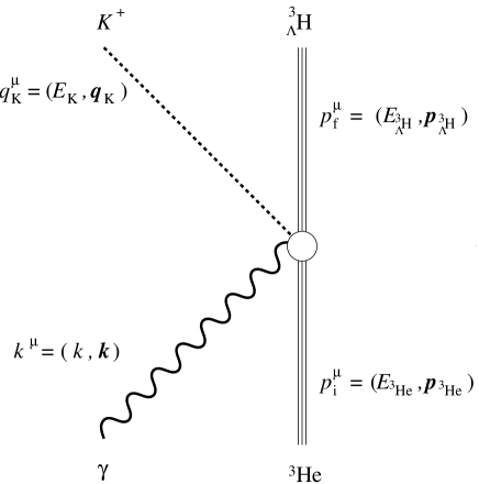
FIG. 1.: Kinematics for kaon photoproduction off ³He.

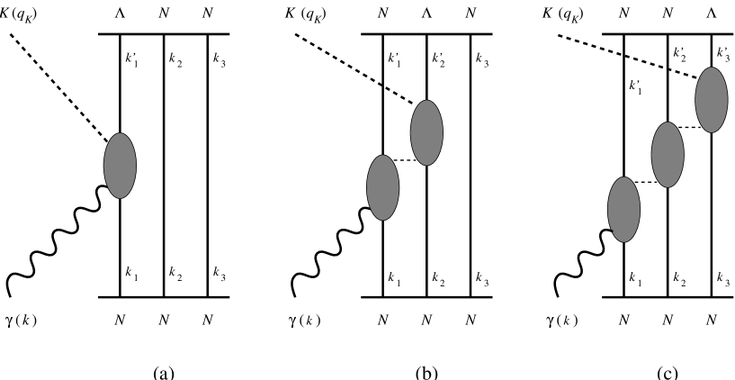
FIG. 2.: Contributions to kaon production on ³He from (a) impulse approximation, (b) and (c) back scattering terms off two or three nucleons, respectively.

FIG. 3.: Momentum transfer ${\vec{Q}}^{\,2}$ (dashed curves) and kaon momentum $q_{K}=|{\vec{q}}_{K}|$ (solid curves) as a function of the photon laboratory energy for 3 different kaon angles.

FIG. 4.: Differential cross section for kaon photoproduction off the proton and ³He as function of kaon angle. The elementary reaction (dotted line) is taken from Ref. [33] and the corresponding experimental datum is from Ref. [36]. The dashed line shows the approximation for production off ³He calculated from Eq. (69), the solid line represents the exact calculation using $S$-waves.

FIG. 5.: The cross section for kaon photoproduction off ³He at three different excitation energies. The dotted curves are obtained from the the calculation with $S$–waves only and the simple hypertriton wave function, the dashed curves are obtained with $S$–waves only and the correlated Faddeev wave function of Ref. [4], while the solid curves show the result after using all of the partial waves and the simple hypertriton wave function.

FIG. 6.: Differential cross sections for kaon photoproduction off ³He predicted by different elementary models. The dash-dotted and the dashed curves are the predictions of the elementary models of Refs. [34] and [35] (set I and set II of Table IV, respectively), the dotted curve is obtained with the coupling constants of set IV [31], and the solid curve is the result for using the model of Ref. [33] (set III). The first two models (dashed and dash-dotted curves) fit the kaon data only up to 1.4 GeV. All curves are calculated by using all partial waves.

FIG. 7.: The influence of Fermi motion on the differential cross section at three different photon energies. The dash-dotted curve is the “frozen nucleon” approximation ($\langle{\vec{k}}_{1}\rangle=0$), the dotted curve is obtained with an average momentum of $\langle{\vec{k}}_{1}\rangle=-\frac{1}{3}{\vec{Q}}$, while the solid curve shows the exact result.

FIG. 8.: The effect of different off-shell assumptions on the cross section calculated at three different energies. The dotted curves have been calculated with the initial nucleon on-shell $\left[k_{1}^{0}=(m_{p}^{2}+{\vec{k}}_{1}^{2})^{1/2}\right]$, the solid curves with the final hyperon on-shell $\left[k_{1^{\prime}}^{0}=(m_{\Lambda}^{2}+{\vec{k}}_{1^{\prime}}^{2})^{1/2}\right]$.

REFERENCES

• [1] K. Miyagawa and W. Glöckle, Phys. Rev. C 48 (1993) 2576.
• [2] A. G. Reuber, K. Holinde, and J.Speth, Nucl. Phys. A 570 (1994) 543; ibid., Czech. J. Phys. 42 (1992) 1115.
• [3] P. M. M. Maessen, Th. A. Rijken, and J. J. de Swart, Phys. Rev. C 40 (1989) 2226.
• [4] K. Miyagawa, H. Kamada, W. Glöckle, and V. Stoks, Phys. Rev. C 51 (1995) 2905.
• [5] T. Hasegawa et al., Phys. Rev. C 53 (1996) 1210.
• [6] B. F. Gibson and E. V. Hungerford III, Phys. Rep. 257 (1995) 349.
• [7] C. Bennhold, Phys. Rev. C 39 (1989) 1944.
• [8] C. Bennhold and L. E. Wright, Phys. Rev. C 39 (1989) 927.
• [9] V. I. Komarov, A. V. Lado, and Yu. N. Uzikov, J. Phys. G 21 (1995) L69.
• [10] L. Tiator, C. Bennhold, and S. S. Kamalov, Nucl. Phys. A 580 (1994) 455.
• [11] R. A. Brandenburg, Y. E. Kim, and A. Tubis, Phys. Rev. C 12 (1975) 1368.
• [12] J. G. Congleton, J. Phys. G 18 (1992) 339.
• [13] M. Juric et al, Nucl. Phys. B 52 (1973) 1.
• [14] G. Keyes et al, Nucl. Phys. B 67 (1973) 269.
• [15] I. R. Afnan and B. F. Gibson, Phys. Rev. C. 47 (1993) 1000; see also Ref. [26].
• [16] G. Keyes et al., Phys. Rev. Lett. 20 (1968) 819; ibid., Phys. Rev. D 1 (1970) 66; G. Keyes, J. Sacton, J. H. Wickens, and M. M. Block, Nucl. Phys. B 67 (1973) 269; R. E. Phillips and J. Schneps, Phys. Rev. Lett. 20 (1968) 1383; ibid., Phys. Rev. 180 (1969) 1307; G. Bohm et al., Nucl. Phys. B 16 (1970) 46.
• [17] J. Dabrowski and E. Fedoryńska, Nucl. Phys. A 210 (1973) 509; B. F. Gibson and D. R. Lehman Phys. Rev. C 10 (1974) 888; H. Roy-Choudhury et al., J. Phys. G 3 (1977) 365; H. Narumi, Nuovo Cimento Lett. 26 (1979) 294; B. F. Gibson and D. R. Lehman, Phys. Rev. C 22 (1980) 2024; S. P. Verma and D. P. Sural, J. Phys. G 8 (1982) 73; I. R. Afnan and B. F. Gibson, Phys. Rev. C 40 (1989) 7; ibid., Phys. Rev. C 41 (1990) 2787.
• [18] T. Warmann and K. Langanke, Z. Phys. A 334 (1989) 221.
• [19] C. Baoqui et al., Chin. J. Phys. 8 (1986) 34; N. N. Kolesnikov and V. A. Kopylov, Sov. Phys. J. 31 (1988) 210.
• [20] S. P. Verma and D. P. Sural, Phys. Rev. C 20 (1979) 781; R. B. Clare and J. S. Levinger, Phys. Rev. C 31 (1985) 2303.
• [21] S. Wycech, Acta Phys. Pol. B 2 (1971) 395.
• [22] J. Dabrowski and E. Fedoryńska in Ref. [17]
• [23] V. G. J. Stoks, R. A. M. Klomp, C. P. F. Terhegen, and J. J. de Swart, Phys. Rev. C 49 (1994) 2950.
• [24] D. R. Tiley, H. R. Weller, and H. H. Hasan, Nucl. Phys. A 474 (1987) 1.
• [25] The value refers to the $\Lambda$-$d$ binding energy. See Ref. [13].
• [26] For the ${}^{3}_{\Sigma}{\mathrm{H}}$ hypertriton the magnetic moment is $0.68~{}\mu_{N}$. See for example C. B. Dover, H. Feshbach, and A. Gal, Phys. Rev. C 51 (1995) 541.
• [27] N. Honzawa and S. Ishida, Phys. Rev. C 45 (1992) 47.
• [28] L. Tiator, A. K. Rej, and D. Drechsel, Nucl. Phys. A 333 (1980) 343; L. Tiator, Nucl. Phys. A 364 (1981) 189.
• [29] L. Tiator and D. Drechsel, Nucl. Phys. A 360 (1981) 208.
• [30] L. Tiator and L. E. Wright, Phys. Rev. C 30 (1984) 989.
• [31] T. Mart, Ph.D. Thesis, Universität Mainz, 1996 (unpublished). The results of the elementary reaction have been published in : T. Mart and C. Bennhold, Few-Body Systems, Suppl. 9 (1995) 369; ibid., Nucl. Phys. A 585 (1995) 369c; T. Mart, C. Bennhold, and C. E. Hyde-Wright, Phys. Rev. C 51 (1995) R1074; T. Mart, C. Bennhold, and L. Alfieri, Acta Phys. Pol. B 27 (1996) 3167.
• [32] J. C. David, C. Fayard, G. H. Lamot, and B. Saghai, Phys. Rev. C 53 (1996) 2613.
• [33] R. A. Williams, C.-R. Ji, and S. R. Cotanch, Phys. Rev. D 41 (1990) 1449; Phys. Rev. C 43 (1991) 452; Phys. Rev. C 46 (1992) 1617.
• [34] R. A. Adelseck and B. Saghai, Phys. Rev. C 42 (1990) 108; Phys. Rev. C 45 (1992) 2030.
• [35] R. A. Adelseck and L. E. Wright, Phys. Rev. C 38 (1988) 1965.
• [36] P. Feller et al., Nucl. Phys. B 39 (1972) 413.
• [37] S. S. Kamalov, L. Tiator, and C. Bennhold, Phys. Rev. C 47 (1993) 941; and references therein.
• [38] S. S. Kamalov, L. Tiator, and C. Bennhold, Nucl. Phys. A 547 (1992) 599.
• [39] S.S. Kamalov, L. Tiator, and C. Bennhold, Phys. Rev. Lett. 75 (1995) 1288.
• [40] A.I. Fix and V.A. Tryasuchev, Yad.Fiz. 60 (1997) 41, translated in: Phys. of At. Nucl. 60 (1997) 35.
• [41] L. Tiator, Ph. D. Thesis, Universität Mainz, 1980 (unpublished).
• [42] W. M. MacDonald, E. T. Dressler, and J. S. O’Connell, Phys. Rev. C 19 (1979) 455.
• [43] D. S. Carman and R. A. Schumacher, ${}^{3}_{\Lambda}{\mathrm{H}}$ Hypernucleus Formation via the Reaction ${}^{3}{\mathrm{H}e}(\gamma,K^{+})X$, A Monte Carlo Study, private communication.
• [44] B. B. Deo and A. K. Bisoi, Phys. Rev. D 9 (1974) 288; P. Dennery, Phys. Rev. 124 (1961) 2000.