Abstract

The universal curve $\sigma/A$ of nuclear photoabsorption is investigated within a Fermi gas model of nuclear matter. An energy range from pion threshold up to 400 MeV is considered. The interactions between nucleon, pion, $\Delta$-isobar and photon are considered in the non-relativistic approximation with corrections of the order $1/M$ taken into account with respect to proton mass. Analytical expressions are obtained, in which the influence of nuclear correlations, two-nucleon contributions and relativistic corrections is studied explicitely. An extension of the model calculation to nucleon knock-out reactions is discussed.

PACS code: 25.20.-x

Keywords: photoabsorption, mesonic exchange currents, nuclear correlation functions

1 Introduction

The phenomenology of nuclear photoabsorption is governed by two characteristic features. First, all nuclei with mass numbers $A$ ranging from 10 to more than 200 obey the same fundamental curve $\sigma(\omega)/A$ for the total photoabsorption cross section devided by $A$ as a function of the photon energy $\omega$. Second, the $\Delta$-isobar excitation of the nucleon is responsible for the main properties of this curve in the energy region between 200 and 400 MeV. Models, which focus on the behaviour of the $\Delta$-isobar in a nuclear environment, namely the $\Delta$-hole calculations [2, 3], have proven to be highly successful in explaining the experimental findings for pion scattering processes [4]. Indeed, on grounds of the $\Delta$-hole formalism a wide variety of pion-nucleus reactions can be described within one consistent framework [5]. In the case of photonuclear reactions, however, serious descrepancies remain, which partially have been accounted for by including non-resonant background terms [6, 7]. Nevertheless, such a procedure, in particular for nuclear photoabsorption, either leads to contradictions with previous $\Delta$-hole results or lacks the complete agreement with experimental data [6]. The question arises, whether theoretical ingredients other than in-medium $\Delta$-hole propagations can lead to a similar degree of accuracy. Therefore it is natural to address the situation from a different point of view asking to what extend the absorption process can be described, when only a very simple $\Delta$-nucleon interaction is used and all additional effects are accounted for in a purely diagrammatic approach. When combined with a simple form of nucleon momentum distribution inside the nucleus, namely a Fermi gas model, this leads to analytical expressions, in which different corrections to this lowest-order approximation can be studied. This is the aim of the present article. In our formalism we follow closely Wakamatsu and Matsumoto [8]. However, we do not introduce a phenomenological potential to account for the deviation of the nucleon wave functions from plane waves, but study the influence of such corrections in a perturbative way, similar to our previous work [9]. In addition, our focus is on the energy-dependence of the total photoabsorption, rather than on the differential cross section as a function of the momentum of the outgoing proton. A characteristic feature of Wakamatsu’s and Matsumoto’s approach is the technically equal treatment of the ($\gamma$,pn) and the ($\gamma$,pp) knock-out process, which allowed them to obtain a natural explanation for the supression of the two-proton knock-out. This characteristic property is also present in our calculation, where it is related to a vanishing trace in spin space. In the last years the ratio ($\gamma$,pp)/($\gamma$,pn) has been investigated in depth within different formalisms. In an extension of Wakamatsu’s and Matsumoto’s work by Boato and Giannini [10], finite-size effects have been calculated and, more recently, a combination of pion exchange and shell-model wave functions was used to investigate this quantity [11]. Currently, two complementary approaches for the description of nuclear knock-out reactions exist. Carrasco and Oset [12] used a diagram-oriented many-body expansion in a Fermi gas. The evaluation of self-energy diagrams leads to an accuracy for medium effects high enough to study knock-out reactions in great detail. With their primary goal being thus different from ours, their formalism does not yield isolated expressions for the resonant and non-resonant parts of the mechanisms of nuclear photoabsorption A different approach is used by the Gent group [13, 14, 15], where the main emphasis lies in the construction of realistic shell-model wave functions, rather than on a microscopic description fully based on the evaluation of Feynman diagrams. As the nuclear photoabsorption is almost insensitive to structural differences between nuclei, the quality of their approach becomes obvious in the investigation of differential cross sections for nucleon knock-out, rather than of photoabsorption.

Nuclear photoabsorption provides an interesting tool to study the interplay between one-nucleon and two-nucleon contributions. We obtained analytical expressions for these contributions, as well as for their resonant and non-resonant parts. This set of results can be used as a starting point to include (and test) further nuclear or nucleonic effects. In Section 2 the basic notations are listed, as well as the interaction terms and the most important model assumptions and approximations, which are present in this calculation. The main results and their most prominent properties, e.g. the effects of relativistic corrections and nuclear structure, are discussed in Section 3, where also the following possible extension of such an approach is considered: As the angular dependence of the two-nucleon process is not very strong (cf. [16]), the different mechanisms contributing to the photoabsorption curve can also be used to understand qualitative features of experimental data for nucleon knock-out processes as a function of the photon energy. In Section 4 some concluding remarks are made, with an emphasis on the applicability of the partial cross sections, whose analytical forms are given in the Appendix.

2 Formalism and Notation

The starting point of our investigation is the static Hamiltonian for the pion-nucleon interaction,

$$H_{\pi NN}=-{f\over m}\;\vec{\sigma}\cdot\vec{\nabla}\;\underline{\tau}\cdot\underline{\phi}$$ (1)

together with a minimal coupling to the photon field. In eq. (1) $m$ is the pion mass. For all coupling constants we use the same notation and values as given in [17], in particular $f^{2}/(4\pi)$=0.08. In eq. (1) underlined symbols denote vectors in (cartesian) isospin space, while an arrow indicates a vector in coordinate space. In the static limit the interactions with the $\Delta$-isobar excitation of the nucleon are determined by the following Hamiltonians (see e.g. [17]):

$$H_{\gamma N\Delta}=-{{ef_{\gamma N\Delta}}\over m}\,\vec{S}^{+}\cdot\left({\vec{\nabla}\times\vec{A}}\right)\,\,T_{z}^{+}$$ (2)

and

$$H_{\pi N\Delta}=-{{f_{\Delta}}\over m}\,\vec{S}^{+}\cdot\vec{\nabla}\underline{T}^{+}\underline{\phi}\,\,,$$ (3)

with the hermitian conjugate to be added in both cases. Here $\vec{S}$ and $\underline{T}$ are the 1/2-to-3/2 transition operators in spin space and isospin space, respectively; $e$ is the proton charge, $e^{2}=1/137$. For the coupling constants we have $f_{\Delta}$=2 and $f_{\gamma N\Delta}$=0.35. In all cases, where high momentum transfers occur at the pion-nucleon vertices we regularize the vertex functions by introducing dipole form factors

$$g_{\pi}(q)={{\Lambda^{2}-m^{2}}\over{\Lambda^{2}-q^{2}}}$$ (4)

as was also done e.g. in [8, 18]. The value for the cut-off parameter $\Lambda$ has been taken to be 800 MeV. This value gives the best agreement of our predictions with the experimental data. In addition, a similar value has been used in [19, 8]. The general expression for the total cross section $\sigma_{1}(\omega)$ of the photoabsorption with one nucleon outside the Fermi sphere and one pion in the final state (one-nucleon process) is of the form

$$\sigma_{1}(\omega)=\int{{{V\,d\vec{p}}\over{(2\pi)^{3}}}}\,\int{{{d\vec{q}}\over{2\varepsilon_{q}(2\pi)^{3}}}}\,{{4\pi}\over{2\omega}}\;\left|{T_{1}}\right|^{2}\times$$

$$2\pi\,\delta\left({\omega+{{p^{2}}\over{2M}}-\varepsilon_{q}-{{(\vec{k}+\vec{p}-\vec{q})^{2}}\over{2M}}}\right)\;n(\vec{p})\;\left[{1-n(\vec{k}+\vec{p}-\vec{q})}\right]\;.$$ (5)

For the total cross section $\sigma_{2}(\omega)$ of the process with two free nucleons in the final state it is given by

$$\sigma_{2}(\omega)=\int{{{V\,d\vec{p}_{1}\,V\,d\vec{p}_{2}}\over{(2\pi)^{6}}}}\,\int{{{d\vec{p}_{3}\,d\vec{p}_{4}\,}\over{(2\pi)^{6}}}}\,{{4\pi}\over{2\omega}}\;\left|{T_{2}}\right|^{2}\,\times$$

$$\delta\left({\omega+{{p_{1}^{2}+p_{2}^{2}-p_{3}^{2}-p_{4}^{2}}\over{2M}}}\right)\,(2\pi)^{4}\,\delta(\vec{p}_{1}+\vec{p}_{2}+\vec{k}-\vec{p}_{3}-\vec{p}_{4})\times$$

$$n(\vec{p}_{1})n(\vec{p}_{2})\left[{1-n(\vec{p}_{3})\;}\right]\left[{1-n(\vec{p}_{4})\;}\right]\;.$$ (6)

The notation for the external momenta is shown in Fig. (1). The function $n(\vec{p})=\theta(p_{F}-\left|{\vec{p}}\right|)$ is the occupation number, $\theta(x)$ is the step function. Furthermore, $V$ is the nuclear volume, $p_{F}$ is the Fermi momentum, $M$ is the mass of the proton, $V$ is the nuclear volume, $V=3\pi^{2}A/(2p_{F}^{3})$, and $\varepsilon_{q}=\sqrt{\left|{\vec{q}}\right|^{2}+m^{2}}$ is the energy of the outgoing pion.

Both amplitudes $T_{1}$ and $T_{2}$ consist of non-resonant and resonant parts, $T_{i}=T_{i}^{(NR)}+T_{i}^{(R)}$. Diagrammatically this decomposition is shown in Fig. (2). The second (crossed) contribution to the resonant part is small due to the big energy denominator and will be skipped in the following. In the energy $\delta$-function in eq. (5) and eq. (6) we will usually not consider the smallest term connected with the kinetic energy of the incoming nucleon, as it is smaller than $p_{F}^{2}/2M\approx 37\,$MeV. Indeed, as we expect its contribution to introduce only a small modification of the actual $p$-dependence in the integrand in (5), we substitute it by its average value $\left\langle{p^{2}}\right\rangle/2M=(3/5)p_{F}^{2}/2M$, which results in an overall shift of the absorption cross section. For the one-nucleon process we find first-order relativistic corrections to be essential for a successful treatment of the absorption process. In the case of the resonant contribution, such corrections are accounted for by making the following substitutions in the vertices [8]:

$$\vec{q} \buildrel{}\over{\longrightarrow}\;\vec{q}-{{\varepsilon_{\vec{q}}}\over{M_{\Delta}}}(\vec{p}+\vec{k}),$$ (7)

$$\vec{k} \buildrel{}\over{\longrightarrow}\;\vec{k}\left({1+{\Delta\over M}}\right)-{\Delta\over M}\,\vec{p}\,,$$ (8)

where $M_{\Delta}$ is the $\Delta$-isobar mass and $\Delta=M_{\Delta}-M$. For the non-resonant part, the corrections give amplitude $T_{1}$ of the following form:

$$T_{1}^{(NR)} = {{\sqrt{2}ef}\over m}\,\left\{{\matrix{{}\cr{}\cr}}\right.i\,\vec{\sigma}\cdot\vec{\varepsilon}\,\left[{1+{{\varepsilon_{q}}\over{2M}}}\right]-{{2i(\vec{\sigma}\cdot(\vec{q}-\vec{k}))(\vec{\varepsilon}\cdot\vec{q})}\over{(\vec{q}-\vec{k})^{2}+m^{2}-(\varepsilon_{q}-\omega)^{2}}}$$ (9)

$$- {{2i(\vec{\sigma}\cdot\vec{q})(\vec{\varepsilon}\cdot(\vec{k}+\vec{p}-\vec{q}))}\over{\,\left[{(\vec{k}+\vec{p}-\vec{q})^{2}-2M\omega-(\vec{p}-\vec{q})^{2}}\right]}}\left.{\matrix{{}\cr{}\cr}}\right\},$$

which corresponds to the production of a $\pi^{-}$. In comparison with [8] we neglected those terms in (9), which modify the result by less than 2 per cent. It should be noted that no free parameters are present in our approach. A certain model dependence exists, however, in the selection of diagrams. We neglect all those diagrams, which are suppressed by some mechanism. In Fig. (3) two examples for suppression mechanisms are given. For Fig. (3a) the contribution is small because in the case of infinite nuclear matter due to momentum conservation the four-momentum of the photon should be equal to that of the outgoing pion, which is impossible. For Fig. (3b) let us consider the case, where the upper two nucleons (incoming and outgoing) are identified. Furthermore, let us select a $\Delta$-isobar as an intermediate state. Then, one has a vanishing trace in spin space:

$$\mbox{Sp}\left[(\vec{S}^{+}\cdot(\vec{k}\times\vec{\varepsilon}))\;(\vec{S}\cdot\vec{q})\right]\,=\,0$$

at $\vec{q}\,=\vec{k}$. Therefore, the contribution in this case vanishes in the non-relativistic limit considered here. As a result of applying such methods to the various diagrams, we have obtained that only those displayed in Fig. (1) should be taken into acount.

3 Results

Explicit evaluation of the diagrams shown in Fig. (1) leads to amplitudes for the one- and two-nucleon contribution to nuclear photoabsorption. Squaring these amplitudes and summing over spin and isospin states of the nucleons by using trace methods as previously [9] one finds the expressions $\left|{T_{1}}\right|^{2}$ and $\left|{T_{2}}\right|^{2}$, which enter into eqs. (5) and (6). It has turned out to be convenient to investigate the resonant and non-resonant parts of each of these contributions separately. This can be done by neglecting the interference terms, which are highly suppressed (cf. Fig. (7)). Shown here exemplary for the resonant parts, one obtains the following expressions, which serve as a starting point for the integrations with respect to nucleon momenta:

$$\sigma_{1}^{(R)}(\omega)={{4e^{2}}\over{27\pi\omega}}\,\left({{{f_{\Delta}f_{\gamma N\Delta}}\over{m^{2}}}}\right)^{2}\int{{{V\,d\vec{p}}\over{(2\pi)^{3}}}}\,\int{d\vec{q}}\;\times$$

$$\delta\left({\omega^{2}+{\omega\over M}\left[{(\vec{p}-\vec{k})^{2}-(\vec{p}-\vec{q})^{2}}\right]-q^{2}-m^{2}}\right)\times$$

$$n(\vec{p}-\vec{k})\;\left[{1-n(\vec{p}-\vec{q})}\right]\,{{3\left[{(\vec{Q}\times\vec{K})\cdot\vec{\varepsilon}}\right]^{2}+Q^{2}(\vec{K}\times\vec{\varepsilon})^{2}}\over{\left({\omega-\Delta-p^{2}/2M}\right)^{2}+\Gamma^{2}/4}},$$ (10)

where

$$\vec{Q}=\vec{q}-{\omega\over{M_{\Delta}}}\,\vec{p}\;,\quad\vec{K}=\vec{k}\left({1+{\Delta\over M}}\right)-{\Delta\over M}\,\vec{p}$$

and

$$\sigma_{2}^{(R)}(\omega)={{16e^{2}}\over{81\pi}}\,\left({{{f_{\Delta}f_{\gamma N\Delta}}\over{m^{3}}}}\right)^{2}\,{\omega\over{\left({\omega-\Delta}\right)^{2}+{{\Gamma^{2}}/4}}}\times$$

$$\int{{{V\,d\vec{p}_{1}\,V\,d\vec{p}_{2}}\over{(2\pi)^{6}}}}\,\int{d\vec{p}_{3}\,d\vec{p}_{4}\,}n(\vec{p}_{1})n(\vec{p}_{2})\left[{1-n(\vec{p}_{3})\;}\right]\left[{1-n(\vec{p}_{4})\;}\right]\times$$

$$\delta\left({\omega-{{p_{3}^{2}+p_{4}^{2}}\over{2M}}}\right)\,\delta(\vec{p}_{1}+\vec{p}_{2}+\vec{k}-\vec{p}_{3}-\vec{p}_{4})\times$$

$$\left\{{{{2a^{2}\left[{a^{2}+3(\vec{\varepsilon}\cdot\vec{a})^{2}}\right]}\over{(a^{2}+m^{2})^{2}}}\,g_{\pi}^{4}(a)+{{2\omega^{2}(\vec{\varepsilon}\cdot\vec{a})(\vec{\varepsilon}\cdot\vec{b})}\over{(a^{2}+m^{2})(b^{2}+m^{2})}}\,g_{\pi}^{2}(a)g_{\pi}^{2}(b)}\right\}$$ (11)

with

$$\vec{a}=\vec{p}_{4}-\vec{p}_{2}\;,\quad\vec{b}=\vec{p}_{1}-\vec{p}_{3}.$$

The analytical expressions for the resulting partial cross sections are given in the Appendix. For the total absorption cross section $\sigma(\omega)$ a comparison with experimental data is shown in Fig. (4). The result of this model calculation compares favorably with the data. The one-nucleon and two-nucleon parts of the cross section are equally important at energies around 250 MeV. As can be seen in this plot, significant features of the data, e.g. the position of the peak, are only obtained due to the interplay between the two mechanisms. As mentioned before, each of the contributions to the full curve in Fig. (4) has a resonant and a non-resonant part. In Fig. (5) and (6) this decomposition is shown for the one-nucleon and the two-nucleon mechanism, respectively. Here it is clearly seen that the non-resonant parts give an important contribution at lower energies. In the two-nucleon case the non-resonant part decreases with energy, while in the one-nucleon process it remains almost constant.

It is interesting to see, in what way the one-nucleon partial cross sections are affected by the use of only the static limit of the interaction. Neglecting the first-order relativistic corrections in the current one has

$$\tilde{\sigma}^{(R)}_{1}(\omega)={{Ae^{2}(f_{\Delta}f_{\gamma N\Delta})^{2}}\over{27m^{2}\left[{\left({\omega-\Delta}\right)^{2}+{{\Gamma^{2}}\over 4}}\right]}}\,\int\limits_{q_{min}}^{q_{max}}{q\,dq}\,\left({1+S_{0}(q)}\right)\times$$

$$\left\{{\left[{\omega^{2}-m^{2}-{{\omega q^{2}}\over M}}\right]+{3\over 2}\left({q^{2}-\left[{q^{2}\left({1+{\omega\over M}}\right)+m^{2}}\right]^{2}{1\over{4\omega^{2}}}}\right)}\right\}$$ (12)

and

$$\tilde{\sigma}^{(NR)}_{1}(\omega)={{Ae^{2}f^{2}}\over{m^{2}\omega^{2}}}\,\int\limits_{q_{min}}^{q_{max}}{q\,dq}\,\left({1+S_{0}(q)}\right)\left[{\matrix{{}\cr{}\cr}}\right.1-{{2m^{2}q^{2}}\over{(q^{2}+m^{2})^{2}}}\times$$

$$\left\{{1-{1\over{4q^{2}\omega^{2}}}\left[{q^{2}\left({1+{\omega\over M}}\right)+m^{2}}\right]^{2}}\right\}\left.{\matrix{{}\cr{}\cr}}\right],$$ (13)

where the integration limits in both cases are given by

$$q_{\min,\max}=\left({1+{\omega\over M}}\right)\,\left\{{\omega\mp\sqrt{\omega^{2}-m^{2}\left({1+{\omega\over M}}\right)\,}}\right\}$$ (14)

and the integrand contains the function

$$S_{0}(q)=-\left({1-{q\over{2p_{F}}}}\right)^{2}\left({1+{q\over{4p_{F}}}}\right)\,\theta(2p_{F}-q).$$ (15)

In Fig. (8) the corresponding cross sections are compared with those resulting from eq. (10) and its non-resonant counterpart. The relativistic corrections lead mainly to a shift of the one-nucleon curve. This effect is essential for obtaining a good agreement with the experimental data. Although no relativistic corrections in the current are included, note that in (12) and (13) terms of that order have been kept in the kinematical contributions to the integrand. As the two-nucleon mechanism gives a comparatively small contribution at higher energies, we neglect relativistic corrections in $\sigma_{2}(\omega)$. This has also been done in [8].

A more difficult problem is the influence, which nucleon correlations inside the nucleus can have on the nuclear photoabsorption process. We investigate this aspect for the non-relativistic forms (12) and (13) of the one-nucleon case. The main reason for doing so is the fact that due to the square of the amplitudes we can express part of the integrand via the standard lowest-order central correlation function of a Fermi gas (see e.g. [20]). The object, which is obtained by diagrammatically squaring the one-nucleon contribution of Fig. (1a), can be coupled to an additional nucleon. In the incoherent case of the diagrammatical square also a further pion exchange can be allowed. The modifications of the correlation function, which occur due to such effects, have been investigated analytically in [9], where a corrected central correlator $S_{C}(q)$ has been constructed. The function $S_{C}$ is given in Fig. (9). By making the substitution $S_{0}(q)\buildrel{}\over{\longrightarrow}S_{C}(q)$ these further correlations can be incorporated effectively. In Fig. (10) the one-nucleon contribution resulting from $S_{C}$ is compared with the original form, in which $S_{0}$ has been used. It can be seen that such medium effects modify the result by about 15 per cent. Naturally, the use of this substitution technique can only be used to obtain an estimate for such a medium-induced modification. A full examination should involve the inclusion of the additional two-and three-nucleon diagrams in eq. (5).

The limit of our approach is certainly reached, when a comparison with differential cross sections is attempted. An extreme case is the comparison with ⁴He, for which a recent measurement of both, the one-nucleon and the two-nucleon channel exists [21]. We compare the calculated average cross section with the data for the differential cross section in c.m. frame, as we expect the angular dependence not to be strong in that frame. The corresponding plot is shown in Fig. (11). Although no full agreement is obtained, it is interesting to note that the general features of the two cross sections are well reproduced, such as the peak positions and the relative size of the two processes. By these means it is possible to unambiguously identify the physical mechanisms behind the data points. A similar degree of agreement is obtained for other data [22].

4 Conclusion

In the present paper we have developed a diagrammatical description of the nuclear photoabsorption process. The main result of our investigation is that the total photoabsorption cross section can be fully understood in terms of a simple physical picture, where point-like nucleons and $\Delta$-isobars interacting via pion exchange are the relevant degrees of freedom. Due to the diagram-oriented formalism and the Fermi gas model as an approximate description of the nucleons in momentum space, we could obtain analytical expressions for all the relevant contributions to the photoabsorption curve. In this way a flexible and efficient description has been obtained, which can be used as a starting point for the investigation of additional effects. Especially in the low-energy part of our calculated curve, the agreement with experiment comes about as a non-trivial interplay between the one-nucleon and two-nucleon contributions. It is worth noting that, as long as a comparatively low cut-off parameter in the vertex form factor is used, there seems to be no need for an explicit diagrammatical inclusion of the $\rho$-meson as an additional mechanism of the nucleon-nucleon interaction. We found relativistic corrections in the case of the one-nucleon process to be crucial for obtaining a good agreement. The aspect of additional nucleon correlations, which can be accounted for as a deviation of the nucleon wave functions from plane waves, deserves some further attention in future investigations. We could estimate the overall effect to be of the order of 15 per cent.

Appendix: Analytical expressions for absorption cross sections

Here we present the explicit expressions for the four contributions to the photoabsorption curve, which have been used to obtain the figures shown in Section 3. As was mentioned earlier, the interference terms between the resonant and the non-resonant contributions are small (cf. Fig. (7)). Therefore, we can write the absorption cross section as a sum of four parts, $\sigma(\omega)=\sigma_{1}^{(NR)}(\omega)+\sigma_{1}^{(R)}(\omega)+\sigma_{2}^{(NR)}(\omega)+\sigma_{2}^{(R)}(\omega)$. First, we deal with the one-nucleon case. In the case of the non-resonant contribution the absorption cross section can be represented in the following form:

$$\displaystyle\sigma_{1}^{(NR)}(\omega)=\frac{3Ae^{2}}{4m^{2}\omega^{2}p_{F}^{3}}\,\int\limits_{\omega_{-}}^{\omega_{+}}dq\int\limits_{l(q)}^{q+p_{F}}dp\,g_{\pi}^{2}(q)\,p\,[p_{F}^{2}-(q-p)^{2}]\times$$

$$\displaystyle G(p,q,\omega)\,\theta(2q\omega-m^{2}-q^{2}-\frac{\omega}{M}p^{2}),$$ (16)

where

$$G(p,q,\omega)\!=\!\left(1+\!\frac{\omega}{2M}\right)^{2}\!-\!\frac{2}{D}\left(\frac{m^{2}}{D}+\frac{\omega}{2M}\right)\left[q^{2}-{1\over{4\omega^{2}}}\left(D+{{\omega}\over M}p^{2}\right)^{2}\right]$$ (17)

and $l(q)=\mbox{Max}[p_{F},|q-p_{F}|]$ , $D=q^{2}+m^{2}$ , $\omega_{\pm}=\omega\pm\sqrt{\omega^{2}-m^{2}}$. In eq. (16) the form factor $g_{\pi}^{2}(q)$ is the same as in (4). Note that the integration with respect to the variable $p$ can easily be performed, but the result is too lengthy to be given here explicitely. The resonant part of the one-nucleon process has the following form:

$$\displaystyle\sigma_{1}^{(R)}(\omega)=\frac{4Ae^{2}}{9\omega p_{F}^{3}}\left(\frac{f_{\gamma N\Delta}}{m^{2}}\right)^{2}\left(1+{\Delta\over M}\right)^{2}\left(1+{\omega\over M}\right)^{2}\int\limits_{-1}^{+1}{dy}\int\limits_{0}^{b}dp\,p^{2}F\times$$

$$\displaystyle\frac{\theta\left(p_{F}^{2}-p^{2}\left(1+\omega/M\right)^{2}-\omega^{2}+2\omega py\left(1+\omega/M\right)\right)}{\left[\omega-\Delta-p^{2}(1+\omega/M)^{2}/2M_{\Delta}\right]^{2}+\Gamma^{2}/4}\;H(p,y,\omega)$$ (18)

where $b=(\omega+p_{F})/(1+\omega/M)$ and the integrand is given by

$$\displaystyle H(p,y,\omega)=2A_{1}\,[\theta(F-p-p_{F})+\theta(F)\,\theta(p-p_{F}-F)\,]+$$

$$\displaystyle[(x+1)A_{1}-{1\over 8}(x-x^{3})A_{2}]\theta(F-|p-p_{F}|)\,\theta(p+p_{F}-F)\,,$$ (19)

with

$$\displaystyle F=\left[\omega^{2}\left(1-\frac{2py}{M}\right)-\frac{m^{2}}{1+\omega/M}\right]^{1/2}\;,\;x=\frac{p^{2}+F^{2}-p_{F}^{2}}{2pF}\,,$$

$$\displaystyle A_{1}=\omega^{2}-2\omega ay+a^{2}\;,\;A_{2}=\omega^{2}(1-3y^{2})+4\omega ay-2a^{2}\;,$$

$$\displaystyle a=\frac{p\Delta}{M}\left(\frac{1+\omega/M}{1+\Delta/M}\right)\,.$$ (20)

The mass difference $\Delta$ between the proton and the $\Delta$-excitation is $\Delta=292$ MeV, the width $\Gamma$ of the $\Delta$-isobar has been taken to be 115 MeV. Again, the integration with respect to $y$ in eq. (18) can be performed analytically, but due to its length the result is not presented here. For the partial cross sections of the two-nucleon case, we obtained the following result:

$$\displaystyle\sigma_{2}^{(NR)}(\omega)+\sigma_{2}^{(R)}(\omega)=$$ (21)

$$\displaystyle\Biggl{\{}\theta(\omega-\varepsilon)\,\theta(5\varepsilon-\omega)\,\Biggl{[}\,\int\limits_{L_{1}(Q)}^{L_{2}(Q)}\Phi(\beta_{1},\,Q)+\int\limits_{L_{2}(Q)}^{2}\Phi(\beta_{2},\,Q)\Biggr{]}+$$

$$\displaystyle\theta(\omega-5\varepsilon)\,\theta(9\varepsilon-\omega)\,\int\limits_{L_{1}(Q)}^{L_{3}(Q)}\Phi(\beta_{1},\,Q)\Biggr{\}}g_{\pi}^{4}(p)\left[G^{(NR)}(p,\omega)+G^{(R)}(p,\omega)\right]dp,$$

where $Q=\sqrt{M\omega}$ , $\varepsilon=p_{F}^{2}/M$ ,

$$\beta_{1}=\arccos\frac{p+p_{F}}{\sqrt{2}Q}\;,\beta_{2}=\arccos\frac{p_{F}}{\sqrt{2}Q}\;.$$

The elementary function $\Phi(\beta,\,Q)$ is

$$\displaystyle\Phi(\beta,\,Q)=\Biggl{\{}\frac{1}{2}(p^{2}-p_{F}^{2})(2Q^{2}+p^{2}-p_{F}^{2})\sin^{2}x\,+Q^{4}(\sin^{4}x-\frac{2}{3}\sin^{6}x)\,+$$

$$\displaystyle p^{2}Q^{2}(x-\frac{1}{4}\sin 4x\,)-\sqrt{8}pQ\,[\frac{1}{3}(2Q^{2}+p^{2}-p_{F}^{2})\sin^{3}x-\frac{2}{5}Q^{2}\sin^{5}x\,]\,+$$

$$\displaystyle\sqrt{8}pQ\,[\frac{1}{3}(2Q^{2}+p^{2}-p_{F}^{2})\cos^{3}x-\frac{2}{5}Q^{2}\cos^{5}x\,]\Biggr{\}}\,\Biggl{.}\Biggr{|}_{x=\beta}^{x=\pi/2-\beta}\,.$$ (22)

The functions in the integrand of eq. (Appendix: Analytical expressions for absorption cross sections), which characterize the resonant and non-resonant part, are given by

$$G^{R}(p,\omega)=\frac{8e^{2}Af_{\gamma N\Delta}^{2}M^{2}}{27\pi^{2}m^{6}p_{F}^{3}}\,\frac{\omega^{2}}{(\omega-\Delta)^{2}+\Gamma^{2}/4}\cdot\frac{p^{4}}{(p^{2}+m^{2})^{2}}\,$$ (23)

and

$$G^{NR}(p,\omega)=\frac{2e^{2}AM^{2}}{\pi^{2}m^{4}p_{F}^{3}}\,\left[1+\frac{m^{4}}{(p^{2}+m^{2})^{2}}\right]\frac{p^{2}}{(p^{2}+m^{2})^{2}}$$ (24)

respectively. In eq. (Appendix: Analytical expressions for absorption cross sections) the integration limits are

$$L_{1}(Q)=Q-p_{F}\;,\quad L_{2}(Q)=\sqrt{2Q^{2}-p_{F}^{2}}-p_{F}$$

and

$$L_{3}(Q)=\sqrt{Q^{2}-p_{F}^{2}}.$$

Figure Captions

Figure 1

Notation for three-momenta of the external particles a) for the one-nucleon process and b) for the two-nucleon reaction. The wavy lines denote photons and dashed lines denote pions. A circle indicates a bound, an arrow a free nucleon.

Figure 2

Diagrammatical forms of the resonant part $T_{i}^{(R)}$ (first two terms) and the non-resonant part $T_{i}^{(NR)}$ (last term) of the amplitude $T_{i}$. These contributions to the $\gamma\pi NN$-interaction enter into the diagrams shown in Fig. (1).

Figure 3

Examples of diagrams, which have not been considered in this approach (cf. discussion in the text).

Figure 4

Comparison of the calculated curve $\sigma(\omega)/A$ for nuclear photoabsorption with the experimental data. The dotted curve is the one-nucleon contribution $\sigma_{1}(\omega)$, while the dashed curve represents the two-nucleon mechanism $\sigma_{1}(\omega)$. The data are taken from Ref. [23]. The empty (full) circles correspond to ²⁰⁸Pb (¹²C) data, while the squares represent data on ¹⁶O.

Figure 5

Resonant (dashed) and non-resonant (dotted) contribution to the one-nucleon reaction (full line). The corresponding analytical expressions $\sigma_{1}^{(R)}(\omega)$, $\sigma_{1}^{(NR)}(\omega)$ and $\sigma_{1}(\omega)$, respectively, can be found in the Appendix.

Figure 6

Same as Fig. (5), but for the two-nucleon reaction. The analytical expressions $\sigma_{2}^{(R)}(\omega)$, $\sigma_{2}^{(NR)}(\omega)$ and $\sigma_{2}(\omega)$, are also given in the Appendix.

Figure 7

Contribution of interference terms. The full (dashed) curve corresponds to the one- (two-) nucleon case. As can be seen from the overall scale, both for $\sigma_{1}$ and $\sigma_{2}$ this contribution is highly suppressed.

Figure 8

Effect of corrections of the order $1/M$ in the one-nucleon mechanism. The full (dashed) curve is with (without) relativistic corrections.

Figure 9

Correlation function $S_{C}$. The dashed curve corresponds to $S_{0}$, while in the dotted curve further two-nucleon correlations and three-nucleon correlations have been included.

Figure 10

Effect of two- and three-nucleon correlation in the case of the non-relativistic one-nucleon part of the photoabsorption cross section. The dashed curve contains only $S_{0}$, while in the full curve $S_{C}$ (cf. Fig. (9)) has been included.

Figure 11

Approximate description of differential cross sections for helium. The differential cross section with respect to the direction of the outgoing proton is shown as a function of the energy of the incoming photon. Data points are taken from [21]. The full curve and filled circles correspond to the one-nucleon process, while the dashed curve and empty circles represent the two-nucleon case.

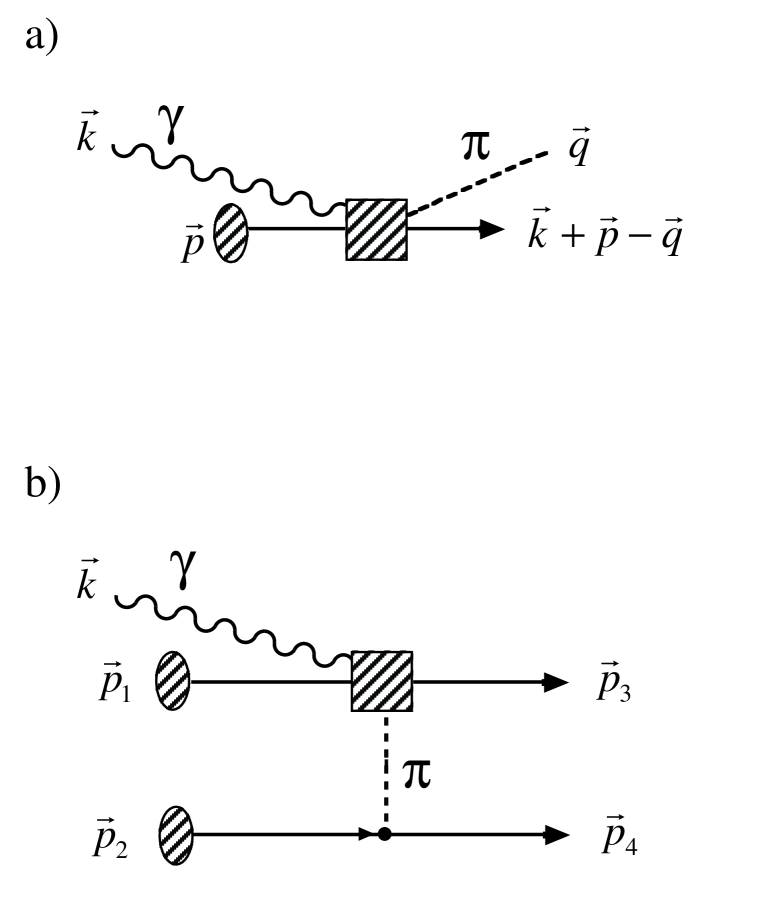
Figure 1:

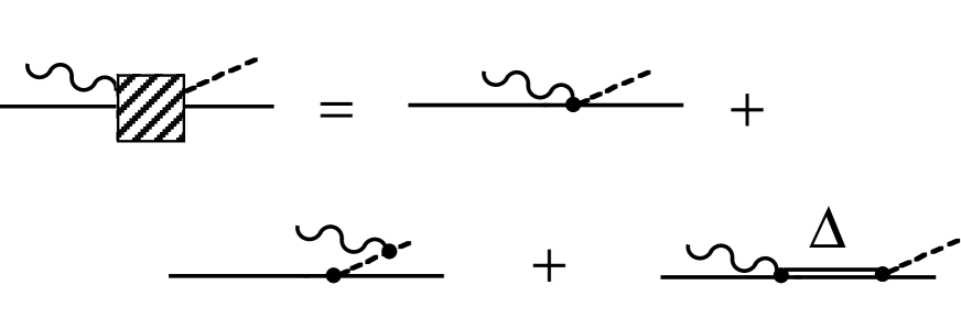
Figure 2:

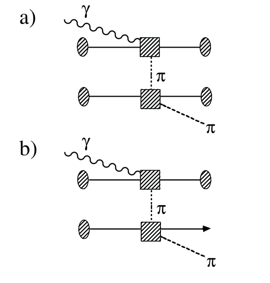
Figure 3:

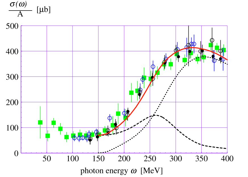
Figure 4:

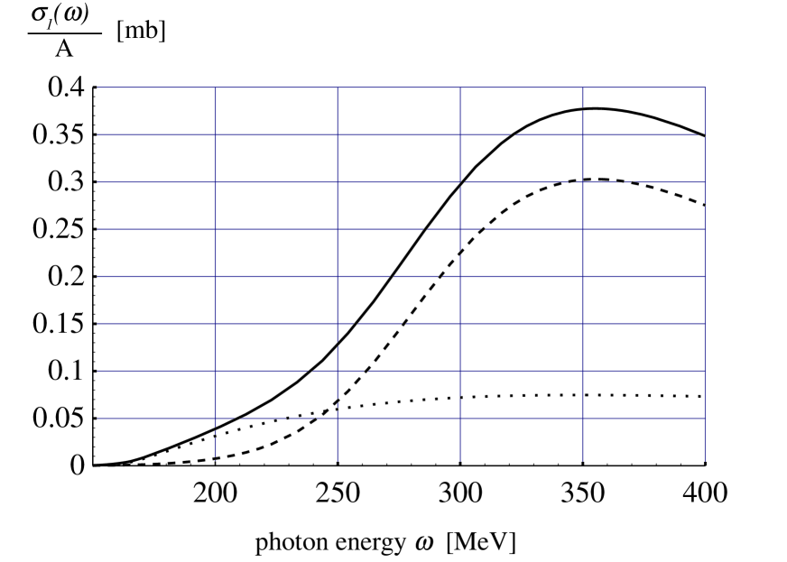
Figure 5:

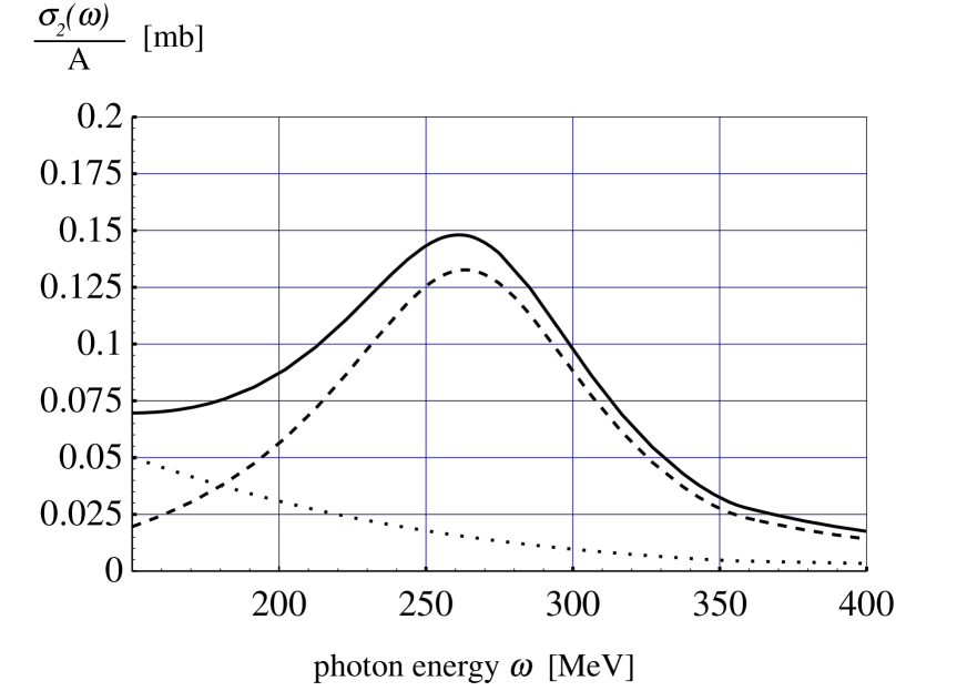
Figure 6:

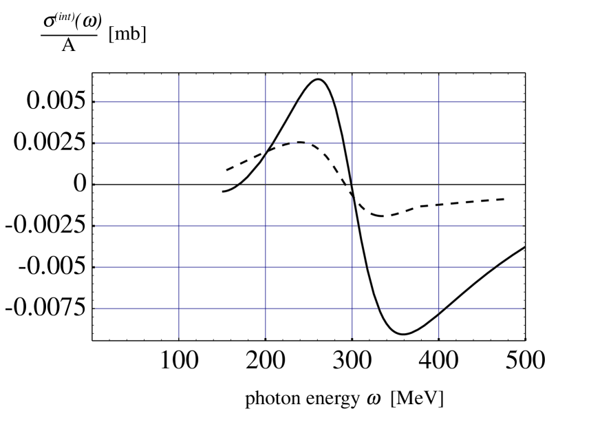
Figure 7:

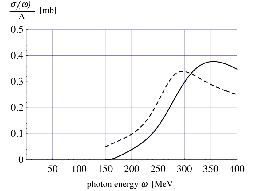
Figure 8:

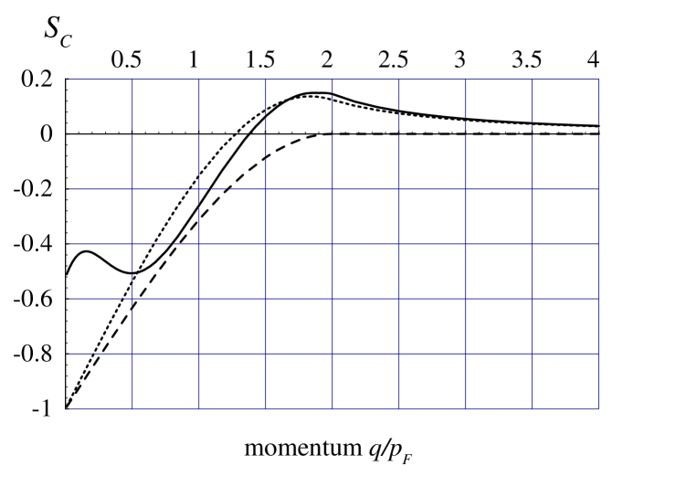
Figure 9:

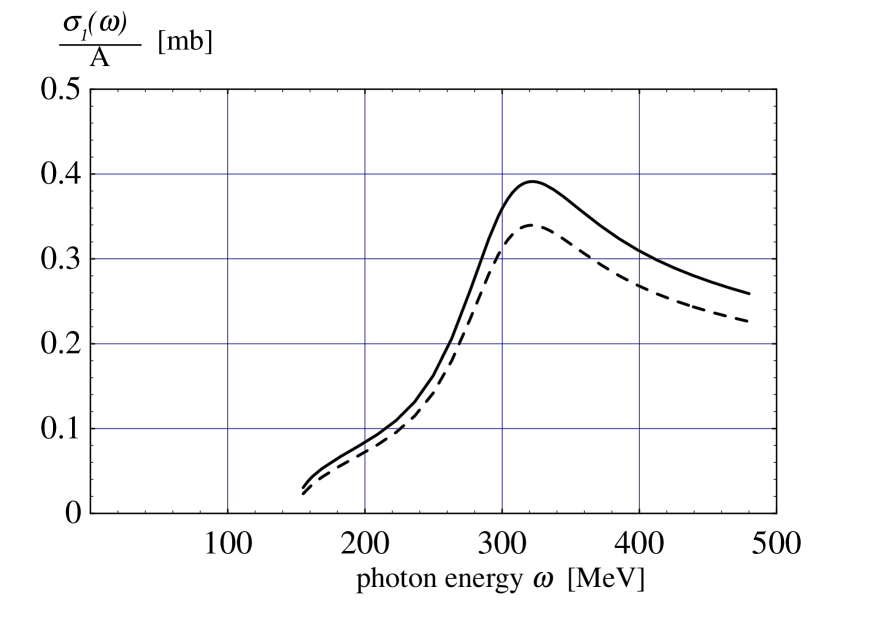
Figure 10:

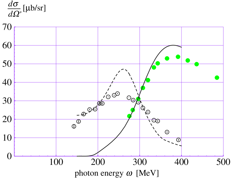
Figure 11:

References

- [1]
- [2] M. Hirata, J. Koch, F. Lenz and E. Moniz, Ann. Phys. 120 (1979) 205
- [3] E. Oset and W. Weise, Nucl. Phys. A329 (1979) 365
- [4] C. Garcia-Recio, L. Salcedo, E. Oset, D. Strottman and M. Lopez-Santodomingo, Nucl. Phys. A526 (1991) 685
- [5] L. Salcedo, E. Oset, M. Vicente-Vacas and C. Garcia-Recio, Nucl. Phys. A484 (1988) 557
- [6] J. Koch, E.J. Moniz and N. Ohtsuka, Ann. Phys. 154 (1984) 99
- [7] E. Oset and W. Weise, Nucl. Phys. A368 (1981) 375
- [8] M. Wakamatsu and K. Matsumoto, Nucl. Phys. A392 (1983) 323
- [9] M.-Th. Hütt and A.I. Milstein, Nucl. Phys. A in press
- [10] L. Boato and M. Giannini, J. Phys. G15 (1989) 1605
- [11] J. Ryckebusch, M. Vanderhaeghen, L. Machenil, M. Waroquier, Nucl. Phys. A568 (1994) 828
- [12] R.C. Carrasco and E. Oset, Nucl. Phys. A536 (1992) 445
- [13] M. Vanderhaeghen, K. Heyde, J. Ryckebusch, M. Waroquier, Nucl. Phys. A595 (1995) 219
- [14] J. Ryckebusch, L. Machenil, M. Vanderhaeghen, V. Van der Sluys and M. Waroquier, Phys. Rev. C49 (1994) 2704
- [15] J. Ryckebusch, L. Machenil, M. Vanderhaeghen, V. Van der Sluys and M. Waroquier, Phys. Lett. B291 (1992) 213
- [16] S. Homma et al., Phys. Rev. C36 (1987) 1623
- [17] T. Ericson, W. Weise, “Pions and Nuclei”, Oxford Univ. Press 1988
- [18] D.O. Riska, Phys. Rep. 181 (1989) 207
- [19] T. Sasakawa, S. Ishikawa, Y. Wu and T. Saito, Phys. Rev. Lett. 68 (1992) 3503
- [20] A. Molinari, Phys. Rep. 64 (1980) 283
- [21] R. Wichmann et al., submitted to Phys. Lett. B
- [22] S. Homma et al., Phys. Rev. Lett. 53 (1984) 2538
- [23] J. Ahrens, Nucl. Phys. A446 (1985) 229c