Phase Transition in the chiral $\sigma$-$\omega$ model with dilatons

Abstract

We investigate the properties of different modifications to the linear $\sigma$-model (including a dilaton field associated with broken scale invariance) at finite baryon density $\rho$ and nonzero temperature $T$. The explicit breaking of chiral symmetry and the way the vector meson mass is generated are significant for the appearance of a phase of nearly vanishing nucleon mass besides the solution describing normal nuclear matter. The elimination of the abnormal solution prohibits the onset of a chiral phase transition but allows to lower the compressibility to a reasonable range. The repulsive contributions from the vector mesons are responsible for the wide range of stability of the normal phase in the ($\mu$, $T$)-plane. The abnormal solution becomes not only energetically preferable to the normal state at high temperature or density, but also mechanically stable due to the inclusion of dilatons.

I Introduction

Although the underlying theory of strong interactions is believed to be known, there is presently little hope to gain insight into the rich structure of the nonperturbative regime at high temperature and nonzero baryon density by solving explicitly the QCD Lagrangian.
Presently, theoreticians try to overcome this unsatisfactory situation by pursuing mainly two methods: First, there is the possibility to solve QCD numerically on a discretized space-time lattice. Reliable results are currently available only for finite temperature and zero baryon density. Efforts to include dynamical fermions on the lattice are still in their infancy and demand a huge amount of computing time. The second possibility is to formulate an effective theory based on symmetries which hopefully reflects the basic features of QCD in a solvable manner. We will focus on the second approach since the consideration of symmetries and scaling may bring deep insight into a complex problem at low computational effort [1].
Gell-Mann and Levy [2] succeeded early with the second kind of ansatz, using the linear $\sigma$-model, in order to describe hadronic properties like pion-nucleon scattering and meson masses.
For the description of nuclear matter saturation properties it is necessary to introduce vector mesons so that the binding energy results from the cancellation of large repulsive and attractive contributions, in analogy to the phenomenologically successful $\sigma-\omega$-model [3]. Early attempts in that direction were done by Boguta who generated the vector meson mass dynamically by coupling scalar fields with vector mesons in the Lagrangian [4]. Unphysical bifurcations could be avoided within their approach, but one was unable to describe the chiral phase transition since the effective nucleon mass tended to infinity for $\rho\rightarrow\infty$. The solution $m_{N}^{\ast}=0$ was confined to $\rho=T=0$. Glendenning investigated the model at high temperatures [5] and found no regime at finite density and nonzero temperatures where chiral symmetry is restored, because of the mechanical instability of the abnormal phase. Mishustin showed that one can simultaneously avoid bifurcations and describe a chiral phase transition at $T$=0, if one introduces an additional field $\chi$, the dilaton, which simulates the broken scale invariance of QCD [6]. By coupling dilatons to vector mesons, one is able to obtain abnormal solutions $\sigma\simeq 0$ without making the vector field massless. Originally, the dilaton field was introduced by Schechter in order to mimic the trace anomaly of QCD in an effective Lagrangian at tree level [7].
In this spirit, many authors applied chiral models to the description of nuclear matter properties [8, 9, 10, 11]. In [12] one was even able to fit and describe finite nuclei as well as the widely used nonlinear version of the Walecka-model [13]. This model fails to describe the chiral phase transition, in contrast to [6], which exhibits a phase transition from a normal state to an abnormal one in the sense of Lee and Wick [14].
The aim of the present paper is to investigate the properties of these modified versions of the linear $\sigma$-model, which claim to give a satisfactory description of nuclear matter ground state properties, at finite temperature within the mean-field ansatz. In part II we present the model which incorporates broken scale and chiral symmetry. Our findings about its phase structure, the chiral phase transition in the ($\mu,T$)-plane, and the temperature dependence of the nucleon effective mass are presented in part III.

II Theory

The linear $\sigma$-model introduced by Gell-Mann and Levy [2] is extended to include an isoscalar vector meson $\omega$ and a scalar, isoscalar dilaton field $\chi$ with positive parity. The scalar field $\sigma$ is the chiral partner of the pion and provides intermediate range attraction. The Lagrangian, which includes the particular ansätze of [6, 15, 10, 12] reads:

$${\cal L} = {\cal L}_{kin}+{\cal L}_{Dirac}-{\cal V}_{vec}-{\cal V}_{0}-{\cal V}_{CSB}$$

$${\cal L}_{kin} = \frac{1}{2}\partial_{\mu}\sigma\partial^{\mu}\sigma+\frac{1}{2}\partial_{\mu}\mbox{\boldmath$\pi$}\partial^{\mu}\mbox{\boldmath$\pi$}+\frac{1}{2}\partial_{\mu}\chi\partial^{\mu}\chi-\frac{1}{4}F_{\mu\nu}F^{\mu\nu}$$ (1)

$${\cal L}_{Dirac} = \overline{N}[i\gamma_{\mu}\partial^{\mu}-g_{\omega}\gamma_{\mu}\omega^{\mu}-g_{\sigma}(\sigma+i\gamma_{5}\mbox{\boldmath$\pi$}\cdot\mbox{\boldmath$\tau$})]N$$ (2)

$${\cal V}_{vec} = -\frac{1}{2}\omega_{\mu}\omega^{\mu}m_{\omega}^{2}[r(\frac{\sigma}{\sigma_{0}})^{2}+(1-r)(\frac{\chi}{\chi_{0}})^{2}]$$ (3)

$${\cal V}_{0} = -\frac{1}{2}k_{0}(\frac{\chi}{\chi_{0}})^{2}(\sigma^{2}+\pi^{2})+\frac{\lambda}{4}(\sigma^{2}+\pi^{2})^{2}+k_{1}(\frac{\chi}{\chi_{0}})^{4}+\frac{1}{4}\chi^{4}\ln\frac{\chi^{4}}{\chi_{0}^{4}}-\frac{1}{2}\delta\chi^{4}\ln\frac{\sigma^{2}+\mbox{\boldmath$\pi$}^{2}}{\sigma_{0}^{2}}$$ (4)

$${\cal V}_{CSB} = -(\frac{\chi}{\chi_{0}})^{2}m_{\pi}^{2}f_{\pi}\sigma\quad.$$ (5)

The field strength tensor reads $F_{\mu\nu}=\partial_{\mu}\omega_{\nu}-\partial_{\nu}\omega_{\mu}$. The original $\sigma$-model is supplemented by nucleons which obey the Dirac equation and by vector mesons whose mass is generated dynamically by the $\sigma$ and $\chi$ fields. We introduce a parameter $r$ which allows the vector meson mass to be generated by $\sigma$ and $\chi$ fields, respectively. The chirally invariant potential is rescaled by an appropriate power of the dilaton field $\chi$ in order to be scale invariant. The effect of the logarithmic term $\sim\chi^{4}\ln\chi$ is two-fold: First, it breaks scale invariance and leads to the proportionality $\theta_{\mu}^{\mu}\sim\chi^{4}$ as can be seen from

$$\theta_{\mu}^{\mu}=4{\cal{L}}-\chi\frac{\partial{\cal L}}{\partial\chi}-2\partial_{\mu}\chi\frac{\partial{\cal L}}{\partial(\partial_{\mu}\chi)}=\chi^{4}\quad,$$ (6)

which is a consequence of the definition of scale transformations [16]. Second, the logarithm leads to a non-vanishing vacuum expectation value for the dilaton field resulting in spontaneous chiral symmetry breaking. This connection comes from the term proportional to $\chi^{2}\sigma^{2}$: With the breakdown of scale invariance the resulting mass coefficient becomes negative for positive $k_{0}$ and therefore the Nambu-Goldstone mode is entered. The comparison of the trace anomaly of QCD with that of the effective theory allows for the identification of the $\chi$ field with the gluon condensate:

$$\theta_{\mu}^{\mu}=\langle\frac{\beta_{QCD}}{2g}G_{\mu\nu}^{a}G^{\mu\nu}_{a}\rangle\equiv(1-\delta)\chi^{4}$$ (7)

The term $\sim\delta\chi^{4}\ln\sigma$ contributes to the trace anomaly and is motivated by the form of the QCD beta function at one loop level, for details see [12]. The last term ${\cal V}_{CSB}$ breaks the chiral symmetry explicitly and makes the pion massive. It is scaled appropriately to give a dimension equal to that of the quark mass term $\sim m_{q}\overline{q}q$ of the QCD Lagrangian.
To investigate the phase structure of nuclear matter at finite temperature we adopt the mean-field approximation [13]. In this approximation scheme, the fluctuations around constant vacuum expectation values of the field operators are neglected:

$$\sigma(x) = \langle\sigma\rangle+\delta\sigma\rightarrow\langle\sigma\rangle$$ (8)

$$\chi(x) = \langle\chi\rangle+\delta\chi\rightarrow\langle\chi\rangle$$ (9)

$$\omega_{\mu}(x) = \langle\omega\rangle\delta_{0\mu}+\delta\omega_{\mu}\rightarrow\langle\omega_{0}\rangle\quad.$$ (10)

The fermions are treated as quantum-mechanical one-particle operators. The derivative terms can be neglected and only the time-like component of the vector meson $\omega\equiv\langle\omega_{0}\rangle$ survives as we assume homogeneous and isotropic infinite nuclear matter. Additionally, parity conservation demands $\langle\mbox{\boldmath$\pi$}\rangle=0$.
It is therefore straightforward to write down the thermodynamical potential of the grand canonical ensemble $\Omega$ per volume $V$ at a given temperature $T$ and chemical potential $\mu$:

$$\frac{\Omega}{V}={\cal V}_{vec}+{\cal V}_{0}+{\cal V}_{CSB}-{\cal V}_{vac}-\frac{\gamma T}{(2\pi)^{3}}\int d^{3}k[\ln(1-n_{k})+\ln(1-\overline{n}_{k})]\quad.$$ (11)

The free energy $f$ is given by

$$f(\rho,T;\sigma,\chi,\omega)=\mu\rho+\frac{\Omega}{V}\quad.$$ (12)

The vacuum energy ${\cal V}_{vac}$ (the potential at $\rho=0$ and $T=0$) has been subtracted. $\gamma$ is the fermionic spin-isospin degeneracy factor (4 for the nuclear medium), $n_{k}$ and $\overline{n}_{k}$ denote the Fermi-Dirac distribution functions for fermions and anti-fermions, respectively:

$$n_{k}(T,\mu^{\ast})=\frac{1}{\exp\left[\left(E^{\ast}(k)-\mu^{\ast}\right)/T\right]+1};\qquad\overline{n}_{k}(T,\mu^{\ast})=\frac{1}{\exp\left[\left(E^{\ast}(k)+\mu^{\ast}\right)/T\right]+1}\quad,$$ (13)

where the single particle energy is $E^{\ast}(k)=\sqrt{k^{2}+{m_{N}^{*}}^{2}}$ with $m_{N}^{\ast}=g_{\sigma}\sigma$. The effective chemical potential reads $\mu^{\ast}=\mu-g_{\omega}\omega$. The meson fields are determined by extremizing $\frac{\Omega}{V}(\mu,T)$:

$$\frac{\partial(\Omega/V)}{\partial\omega} = -\omega m_{\omega}^{2}[r(\frac{\sigma}{\sigma_{0}})^{2}+(r-1)(\frac{\chi}{\chi_{0}})^{2}]+g_{\omega}\rho=0$$ (14)

$$\frac{\partial(\Omega/V)}{\partial\chi} = -\omega^{2}\frac{m_{\omega}^{2}(1-r)}{\chi_{0}^{2}}\chi-k_{0}\frac{\chi}{\chi_{0}^{2}}\sigma^{2}+(4\frac{k_{1}}{\chi_{0}^{4}}+1+\ln\frac{\chi^{4}}{\chi_{0}^{4}}-2\delta\ln\frac{\sigma^{2}}{\sigma_{0}^{2}})\chi^{3}-2m_{\pi}^{2}f_{\pi}\frac{\chi\sigma}{\chi_{0}^{2}}=0$$ (15)

$$\frac{\partial(\Omega/V)}{\partial\sigma} = -\omega^{2}\frac{m_{\omega}^{2}r}{\sigma_{0}^{2}}\sigma-k_{0}(\frac{\chi}{\chi_{0}})^{2}\sigma+\lambda\sigma^{3}-\delta\frac{\chi^{4}}{\sigma}-m_{\pi}^{2}f_{\pi}(\frac{\chi}{\chi_{0}})^{2}+g_{\sigma}\rho_{s}=0\,,$$ (16)

where the scalar density is given by

$$\rho_{s}=\gamma\int\frac{d^{3}k}{(2\pi)^{3}}\frac{m_{N}^{\ast}}{E^{\ast}}(n_{k}+\overline{n}_{k})\quad.$$ (17)

The vector field $\omega$ can be solved explicitly in terms of $\sigma$ and $\chi$, yielding

$$\omega=\frac{g_{\omega}\rho}{m_{\omega}^{2}(r(\frac{\sigma}{\sigma_{0}})^{2}+(r-1)(\frac{\chi}{\chi_{0}})^{2})}\qquad.$$ (18)

Note, that in $\omega_{0}$-direction the pressure is minimal, since the temporal and spatial components of the vector field enter with opposite sign and only the latter are dynamical variables.
In addition, one has to determine the baryon density at a given chemical potential via the equation

$$\rho=\gamma\int\frac{d^{3}k}{(2\pi)^{3}}(n_{k}-\overline{n}_{k})\quad.$$ (19)

The energy density and the pressure are given by

$$\epsilon = {\cal V}_{vec}+{\cal V}_{0}+{\cal V}_{CSB}-{\cal V}_{vac}+\frac{\gamma}{(2\pi)^{3}}\int d^{3}k(E^{\ast}(k)-\mu^{\ast})\stackrel{{\scriptstyle\rho=0}}{{\longrightarrow}}\epsilon_{SB}=\gamma\sigma_{SB}T^{4}$$ (20)

$$p = -\frac{\Omega}{V}\stackrel{{\scriptstyle\rho=0}}{{\longrightarrow}}p_{SB}=\frac{1}{3}\gamma\sigma_{SB}T^{4}$$ (21)

Here, the index $SB$ denotes the corresponding quantities in the Stefan-Boltzmann limit with $\sigma_{SB}=7\pi^{2}/120$. The limit $T\rightarrow 0$ can be taken straightforwardly, using

$$\lim_{T\rightarrow 0}T\ln(1-n_{k})=E^{\ast}(k)-\mu^{\ast}\quad.$$ (22)

Applying the Hugenholtz-van Hove theorem [17], the Fermi surface is given by

$$E^{\ast}(k_{F})=\sqrt{k_{F}^{2}+(g_{\sigma}\sigma)^{2}}=\mu^{\ast}\quad.$$ (23)

The scalar density and the baryon density can be determined analytically, yielding

$$\rho_{s} = \frac{\gamma m_{N}^{\ast}}{4\pi^{2}}\left[k_{F}E_{F}^{\ast}-m_{N}^{\ast 2}\ln(\frac{k_{F}+E_{F}^{\ast}}{m_{N}^{\ast}})\right]$$ (24)

$$\rho = \gamma\int_{0}^{k_{F}}\frac{d^{3}k}{(2\pi)^{3}}=\frac{\gamma k_{F}^{3}}{6\pi^{2}}\quad.$$ (25)

If the dynamical vector meson mass is considered as being generated by $\chi$ alone and if $\delta$ is set to zero, it is possible to solve equation 16 analytically:

$$\chi=\chi_{0}\sqrt{\frac{\lambda\sigma^{3}+g_{\sigma}\rho_{s}}{k_{0}\sigma+m_{\pi}^{2}f_{\pi}}}\quad.$$ (26)

Thus, the numerical procedure is simplified to finding the root of a nonlinear equation of one independent variable, namely $\sigma$. This allows for a visualization of the phase structure at zero temperature.
In order to describe hadrons and nuclear matter within the model, the appropriate model parameters must be chosen. The pion mass is fixed at the value $m_{\pi}=138$ MeV which determines the parameter $k_{0}$ from the following relation:

$$k_{0}=\lambda f_{\pi}^{2}-\delta\frac{\chi_{0}^{4}}{f_{\pi}^{2}}-m_{\pi}^{2}\quad.$$ (27)

This equation can be obtained from equation 16 by setting $\rho=T=0$ and using $\sigma_{0}=f_{\pi}$. In addition, one has to ensure that also in the vacuum $\frac{\partial(\Omega/V)}{\partial\chi}=0$. This leads to the determination of $k_{1}$:

$$k_{1}=\frac{f_{\pi}^{2}}{4}(2m_{\pi}^{2}+k_{0}-\frac{\chi_{0}^{4}}{f_{\pi}^{2}})\quad.$$ (28)

The Goldberger-Treiman relation can be used at the tree level to fix the coupling of the nucleons to the $\sigma$ field, $g_{\sigma}=\frac{m_{N}}{f_{\pi}}$.
The vector meson mass is set to $m_{\omega}=783$ MeV and $\lambda$ is a free parameter which determines the $\sigma$-mass. The remaining two parameters ($g_{\omega}$ and $\chi_{0}$) are fitted to the ground state nuclear matter binding energy $E_{B}=\epsilon/\rho-m_{N}=-16$ MeV with zero pressure at equilibrium density $\rho_{0}=0.15$ fm^-3. Several parameter sets have been tested. They are listed in table 1. The first three rows correspond to the version of [6] with $\delta=0$, which we will call hereafter the minimal model. There, the vector mesons are coupled only to the dilatons. Concerning the compressibility $K$, which should be around 200-400 MeV [18], we find that a small quartic self-interaction of the $\sigma$ corresponding to small $\lambda$ is to be preferred in this model. If the logarithmic potential is included proportional to $\delta$ [12], it is possible to set $\lambda=0$ and therefore to lower the compressibility to reasonable values. Note, however, that the effective nucleon mass at $\rho_{0}$, which should be $\approx 0.7m_{N}$, tends to increase with decreasing $\lambda$.

III Results

In order to study the properties and the impact of the different modifications to the minimal chiral model on the observables, we focus first on the phase structure at $T$=0 before discussing our findings at finite temperature.
The influence of the explicit chiral symmetry breaking term on the phase structure of nuclear matter is checked by computing the binding energy of nuclear matter versus the $\sigma$ field for normal nuclear density $\rho=\rho_{0}$ (Fig. 1 above) and $\rho=4\rho_{0}$ (Fig. 1 below) in the minimal version of the chiral model with $\delta=0$. The first and the second column correspond to the model with and without explicit symmetry breaking, respectively. According to [6], the phase curve in Fig. 1a exhibits the appearance of three distinct minima: The first one is at $m_{N}^{\ast}\simeq 0.6-0.7m_{N}$ (the exact value depends on the parametrization) which we denote as the ’normal’ minimum. Besides a metastable minimum at roughly $m_{N}^{\ast}\simeq 0.2m_{N}$, which does not play a significant role (it never becomes the energetically lowest state), there is a third minimum corresponding to nearly vanishing effective nucleon mass ($0.02m_{N}$). This is the ’abnormal’ minimum which becomes the energetically preferable state for large densities (Fig. 1b). There, a phase transition takes place into a chiral phase where the nucleon effective mass as order parameter is nearly vanishing. Fig. 1c shows that the exclusion of explicit symmetry breaking effects in the Lagrangian does change the phase structure even at $\rho_{0}$ significantly. Although the properties of the matter at the normal minimum are not affected, the exclusion of the explicit symmetry breaking term eliminates the abnormal solution entirely and therefore a chiral phase transition does not occur.
There is another constraint for the existence of an abnormal phase: A pure $\omega$-$\sigma$-coupling without a dilaton admixture ($r=1$) eliminates the abnormal solution. This can be seen as follows: For $r=1$, an additional term enters the numerator of equation 26 yielding

$$\chi=\chi_{0}\sqrt{\frac{\lambda\sigma^{3}+g_{\sigma}\rho_{s}-g_{\omega}^{2}\rho^{2}m_{\omega}^{2}\sigma_{0}^{2}/\sigma^{3}}{k_{0}\sigma+m_{\pi}^{2}f_{\pi}}}\quad,$$ (29)

so that $\chi$ diverges for $\sigma\rightarrow 0$. In fact, irrespectively of which parametrization one uses, $\chi$ becomes imaginary as soon as $\sigma\stackrel{{\scriptstyle<}}{{\sim}}0.4m_{N}$. No solution is possible for smaller $\sigma$ values, where an abnormal minimum would occur. We tried to lower the compressibility in the minimal version of the chiral model presented in [6] and found a lower bound of $\lambda$=150 necessary to ensure that the abnormal state is not the energetically lowest one at normal nuclear matter density. If an abnormal minimum exists, at ground state density, the $\sigma^{4}$-term has to contribute strongly and the compressibility cannot be lowered to observed values. A way out is to permit $\delta\neq 0$ [12], which mimics the contribution of quark pairs to the QCD $\beta$-function at one loop level: Then, it is possible to break the symmetry spontaneously even without a quartic self-interaction, i.e. with $\lambda=0$. The compressibility is thus lowered to reasonable values, without abnormal or chiral phase restoration occuring at high energy densities.
Let us now turn to finite temperatures. Here, the analysis gets more involved: three coupled equations have to be solved simultaneously. At low temperatures, the model exhibits a liquid-gas phase transition as can be seen from Fig. 2 (using parameter set V). The main difference between the minimal and the extended model sets in at high temperatures and densities because of the existence of the abnormal solution in the minimal model. Fig. 3 shows a contour plot of the free energy at $T$=170 MeV and at ground state density $\rho_{0}$ using set I. The abnormal minimum (at nearly vanishing nucleon effective mass) and a normal phase (at $m_{N}^{\ast}\simeq 0.7m_{N}$) are clearly visible. At normal nuclear density, a chiral phase transition occurs at $T$=168 MeV. The phase transition is of first order, since the change in the free energy is discontinuous.
The calculation of the phase boundary in the ($\mu$, $T$)-plane yields surprising results if the minimal model is used (Fig. 4, Set I). Along the boundary shown in the figure the difference between the pressure of the abnormal and normal solutions vanishes, i.e., the transition to the chiral phase takes place. The transition at $T$=0 was already noted in [6].
However, the extension to finite temperatures does not lead to a closed phase boundary, regardless which parametrization one uses (see, e.g., triangles with $\lambda=300$, black circles with $\lambda=220$). The abnormal solution is stable at high temperatures or at high baryon densities, but not for both. This can be seen from Fig. 5, where at four particular points in the ($\mu,T$)-plane of Fig. 4 the pressure as a function of the $\sigma$ field is drawn. The abnormal maximum of the pressure is flat (Fig. 5a,b) or it disappears completely (Fig. 5c) far away from the phase transition line. It becomes a well pronounced maximum with a high barrier to the normal state in the vicinity of the phase transition region (Fig. 5d).
The result that one has an open phase boundary within the plotted ($\mu$, $T$)-regime is unusual and counter-intuitive. In contrast, in [20] a closed phase boundary was obtained by investigating the linear $\sigma$-model including neither repulsive contributions from $\omega$-meson exchange nor dilatons. To simulate this calculation within our model we keep all parameters constant and change only the $\omega$-coupling to $g_{\omega}=6$ (black dots) and $g_{\omega}=0$ with varying gluon condensate (white trangles) and $g_{\omega}=0$ with the gluon condensate frozen at its vacuum value (white circles). The presence of the dilaton field does not lead to the fan out of the phase transition curve. Nevertheless, it has the considerable effect to shift the transition points to roughly twice the values as compared to the ’non-frozen’ case. Switching from $g_{\omega}=0$ to $g_{\omega}=6$ and to $g_{\omega}=8.2$, the phase boundary spreads out to higher densities and temperatures. Therefore, the reason for the unusual form of the phase boundary is the repulsive contribution due to the $\omega$-meson exchange.
At that point we should emphasize that our results are obtained in the framework of the mean-field approximation. The inclusion of quantum fluctuations in the meson fields could change our findings qualitatively. This wil be investigated elsewere [21]. Inclusion of resonances might lead to the closure of the boundary as was observed in [22] and [5] that taking these additional degrees of freedom into account, the critical densities and temperatures decrease. Another possibility to get a closed phase boundary might be the inclusion of a quartic self interaction for the vector meson, $(\omega_{\mu}\omega^{\mu})^{2}$, yielding $\omega\sim\rho^{1/3}$: the amount of repulsion at high densities is lowered. A detailed analysis will be found in [28].
The extended chiral model with $\delta\neq 0$ does not show a chiral phase transition at all. The nucleon effective mass increases at high density and temperature, as can be seen in Fig. 6. A similar behaviour of the effective nucleon mass can be found for the normal phase of the minimal model. The difference to the extended model comes from the fact that -according to the phase diagram of figure 4- a transition from high to low effective masses or vice versa can be found.
In contrast to finite baryon density, almost no temperature dependence of the effective nucleon mass in the normal phase is found at $\rho=0$ until the phase transition takes place. In addition, the abnormal phase at $\rho=0$ differs qualitatively from the one at finite density. There, the two fields $\sigma$ and $\chi$ vanish exactly, irrespective of the explicit symmetry breaking term, whereas at finite baryon density the $\chi$ field in the abnormal phase remains finite, as can be seen in Fig. 3 (there, $\chi\simeq 84$ MeV). When $\sigma=0$, the scalar density vanishes and from equation 26 it follows that the $\chi$ field becomes zero. Because the baryonic density vanishes, no singularity occurs if $\chi=0$.
It is also interesting to compare the high temperature phase transition of the Walecka-model at zero density studied in [27] with that of the minimal chiral model (Fig. 7). One observes that at high temperatures the energy density and the pressure asymptotically approach the limit of a noninteracting fermion gas. As in [27], we find that the energy density decreases with high temperatures whereas the pressure reaches its asymptotic limit from below.
Similar results concerning the properties of the linear $\sigma$-model at finite temperature were obtained in [5], which in our terminology would be the minimal model with a pure $\sigma-\omega$-coupling and no dilatons. However, there is an important difference, which results from the inclusion of the dilaton field $\chi$: Whereas in [5], the abnormal phase is always mechanically unstable (the pressure decreased with compression), leading to the result that no region in the ($\rho$, $T$)-plane existed where chiral symmetry was restored, we find here that the abnormal or chiral restored phase is always mechanically stable (Fig. 8). The difference to Glendenning’s work originates from the $\omega-\chi$- rather than $\omega-\sigma$-coupling. In contrast to [25], where it is argued that the influence of the dilaton is negligible at finite density because of its high mass, we find the variation of the condensate $\chi$ to be essential for a mechanically stable abnormal phase. Similar results pointing to the importance of the dilaton field in nuclear matter are also obtained in [26], where the Walecka model including dilatons was studied.
The final question to be addressed is, whether the interesting (T,$\rho$)-regions can be reached in relativistic heavy ion collisions. For a rough estimate, we solve the Rankine-Hugoniot-Taub adiabate (RHTA), which can be used as a first approximation for the description of nearly central collisions of fast heavy nuclei [29, 30]. The thermodynamic quantities calculated for the compression stage of the collision are shown in figure 9. The gap in the solution of the abnormal branch comes from the disappearance of the abnormal maximum in the corresponding region (see, i.e, Fig. 5).
The evolution of the system in the subsequent expansion is calculated by the isentropes starting from a point on the Taub-adiabate (Fig. 10a). A minimum at $S/A\leq 2$ in the trajectory allows for the mechanical instability, which is suggested to cause multifragmentation. The expansion of the system from an abnormal initial state through a mixed phase into the normal state is shown in Fig. 10b. Even though we cannot reach the abnormal phase with the shockfront model, it might be possible, i.e. with the fireball model with $\rho=2\gamma_{CM}\rho_{0}$.

IV Summary and outlook

The properties of the linear $\sigma$-model presented in [6, 10, 15, 12] are studied at finite temperature $T$ and nonzero baryon density $\rho$. At nuclear matter saturation density $\rho_{0}$, the minimal model of [6] exhibits two phases (the abnormal one at nearly vanishing nucleon mass and the normal phase at $m_{\ast}\simeq 0.7m_{N}$), which allows for a phase transition at high temperatures or high densities. The presence of vector mesons leads to an open phase boundary, and the inclusion of dilatons makes the abnormal phase also mechanically stable. However, in the model abnormal solutions at $\rho_{0}$ exist only at unphysically high values of the compressibility (K $\stackrel{{\scriptstyle>}}{{\sim}}1400$ MeV). Therefore, the abnormal phase should be eliminated by either including a $\omega-\sigma$-coupling or by replacing the quartic self-interaction with a logarithmic term ($\delta\neq 0$). In this case, no chiral phase transition can be found since the nucleon effective mass as order parameter increases at high densities and temperatures. It remains a challenge to construct a reasonable chiral model for nuclear matter which allows for the study of phase transitions. First calculations done in an extension of the model to SU$(3)$ are encouraging [28].

FIG. 1.: Binding energy versus $\sigma/\sigma_{0}$ with (left) and without (right) explicit symmetry breaking (ESB) for saturation density $\rho_{0}$ (above) and $4\rho_{0}$ (below) calculated with Set I

FIG. 2.: Liquid-gas phase transition in the chiral $\sigma-\omega$ model (calculated with Set V).

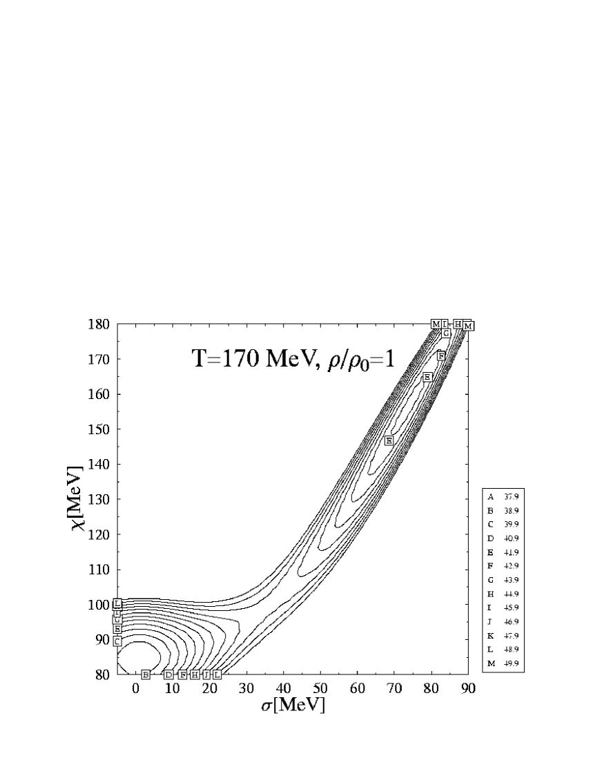
FIG. 3.: A contour plot of the free energy in the ($\chi,\sigma$)-plane. The abnormal and normal minimum are visible.

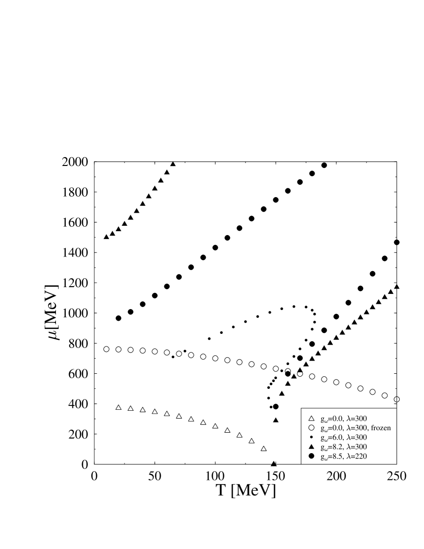
FIG. 4.: Phase transition points for different values of the N-$\omega$ coupling constant in the ($\mu$, T)-plane

FIG. 5.: Pressure versus the scalar field $\sigma$. The abnormal solution does not exist far from the phase transition line. The barrier between normal and abnormal phase becomes well pronounced near the phase transition region.

FIG. 6.: Effective nucleon mass versus temperature (above) and density (below)

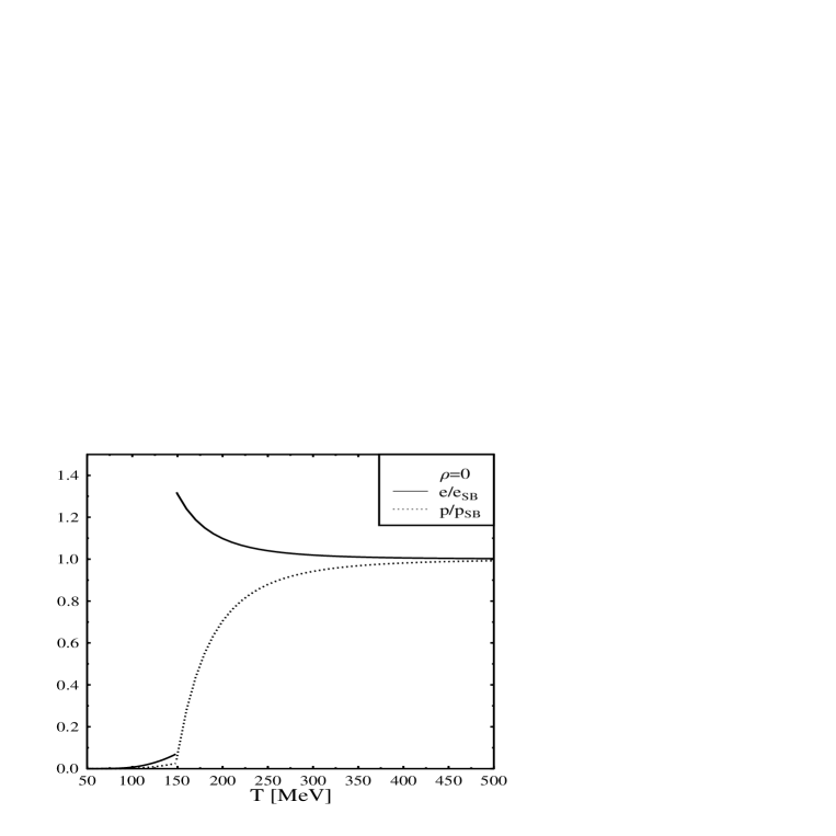
FIG. 7.: High temperature limit of the energy density and pressure for zero density (Set I).

FIG. 8.: Pressure as a function of density (left) and chemical potential (right), calculated with Set I.

FIG. 9.: Temperature, density and entropy per baryon as a function of the bombarding energy E_Lab (Set I).

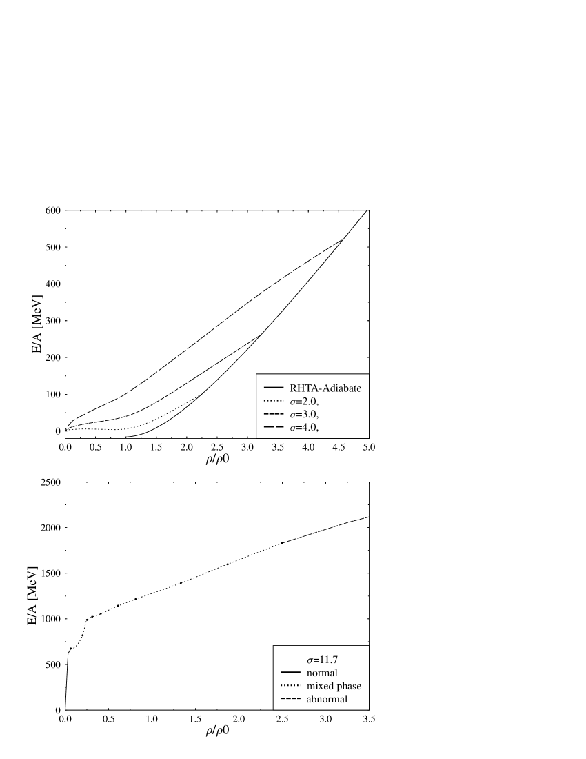
FIG. 10.: Expansion of a compressed state along different isentropes starting from the normal phase (a) and from the abnormal phase (b), respectively.

TABLE I.: Different parameter sets which describe nuclear matter saturation

Set	$\lambda$	$\chi_{0}$ (MeV)	$g_{\omega}$	$m_{N}^{\ast}/m_{N}$	$\chi/\chi_{0}$	$K$ (MeV)	r	$33\delta$	$m_{\pi}(MeV)$
I	300	189.3	8.2	0.66	0.71	1464	0	0	138
II	220	188.7	8.2	0.67	0.71	1403	0.5	0	138
III	40	331.7	6.8	0.78	0.94	669	1	0	138
IV	0.84	392.9	5.9	0.84	0.99	387	1	4	0
V	0	372.5	7.6	0.80	0.98	356	0.5	4	0