NBI–96–25

September, 1996

Many–Particle Correlations in Relativistic Nuclear Collisions

Henning Heiselberg

NORDITA, Blegdamsvej 17, DK-2100 Copenhagen Ø., Denmark

and Axel P. Vischer

Niels Bohr Institute,Blegdamsvej 17, DK-2100, Copenhagen Ø, Denmark.

Abstract

Many–particle correlations due to Bose-Einstein interference are studied in ultrarelativistic heavy–ion collisions. We calculate the higher order correlation functions from the 2–particle correlation function by assuming that the source is emitting particles incoherently. In particular parametrizations of and relations between longitudinal, sidewards, outwards and invariant radii and corresponding momenta are discussed. The results are especially useful in low statistics measurements of higher order correlation functions. We evaluate the three–pion correlation function recently measured by NA44 and predict the 2–pion–2–kaon correlation function. Finally, many particle Coulomb corrections are discussed.

I Introduction

Particle interferometry is an indispensable tool for the study of the space-time structure of the emitting source created in ultrarelativistic heavy–ion collisions. Recent experiments  [1, 2, 3] not only enable us to obtain a good spatial resolution in all 3 dimensions for the 2–pion correlation function, but also provide large enough data samples to investigate many–pion correlations [4].

The basic issue one wants to address and resolve with three or more particle interferometry is, if there exist additional correlations beyond Bose-Einstein (BE) interference of identical particles from an incoherent source. In this paper we predict the three– and more particle correlation functions on these assumptions and explore whether the two-body correlation function suffices to describe the many–particle system. In particular we compare to recent data on the three-body correlation function. Any deviation found experimentally from this prediction signals new physics like, e.g., coherent emission or true higher order correlations. We use the measured two–particle correlation functions as input and therefore obtain a parameter free prediction of higher order correlation functions.

Our starting point are the three–parameter fits to the two–pion correlation function $C_{\rm 2}$. This correlation function depends on the momentum difference, ${\bf q}$, of the pion pair. In section 2 we provide a simple method for calculating many-body correlation functions due to Bose-Einstein interference between identical particles emitted incoherently from a source and discuss to which degree they can be determined from the two-body correlation function alone. To demonstrate our method, we reduce in section 3 the dependence on the three–relative momenta to a dependence on only the Lorentz invariant relative momentum and compare our result to the corresponding one–parameter experimental fit and data [1]. The resulting expression is approximated by an expansion in the deviations of the pion source from a spherical shape. We show that the lowest order corrections are sufficient to reproduce the full expression.

In section 4 we proceed to evaluate the three–pion correlation function $C_{\rm 3}$ and compare it with recent results [4]. We find that within the experimental errors the prediction based only on three–pion correlations can reproduce the data. Finally in section 5 we discuss Coulomb effects and present a simple way to correct many particle correlation functions. We conclude with a summary of our results.

II BE interference and many-body correlation functions

We want to outline a general calculation of many-body correlation functions which can be done elegantly for relativistic heavy–ion collisions. The method reproduces in a simple calculation the two-, three- and four-body correlation functions found previously by diagrammatic techniques [12]. Readers familiar with the results may skip this section.

The approximations, that we will employ, are:

• incoherent source, i.e., particles are emitted independent of each other and carry no phase information as is the case in (coherent) stimulated emission. This is a strong assumption, which can only be tested by comparison to experimental data. Existing two-body correlation functions are well described by fully incoherent pion and kaon emission (see, e.g., [10]).

• plane wave propagation after emission. This assumes that Coulomb repulsion can be corrected for (see, e.g., [14] and section 5) and that other final state interactions are negligible.

• particle momenta are much larger than relative momenta. This is a good approximation as the momenta of particles emerging from relativistic heavy ion collisions are larger than the typical transverse momenta which are $\sim 300$MeV/c. In comparison the interference occur for relative momenta, $q$, less than the inverse of the source size, $R\simeq 3-5$fm, and so $q\raisebox{-2.15277pt}{$\stackrel{{\scriptstyle<}}{{\sim}}$}\hbar/R\sim 50$MeV/c.

• large multiplicity. The multiplicity in high energy nuclear collision is hundreds or thousands of particles which is much larger than the number of particles we want study correlations for.

The N-body correlation function relates directly to measured cross-sections

$$C(k_{1},k_{2},..,k_{N})=\sigma^{N-1}\frac{d^{3N}\sigma/d^{3}k_{1}d^{3}k_{2}...d^{3}k_{N}}{d^{3}\sigma/d^{3}k_{1}....d^{3}\sigma/d^{3}k_{N}}$$ (1)

where $k_{1},...,k_{N}$ are the four-momenta of the N particles.

The wave function for a particle emitted at the source point $x_{i}$ with momentum $k_{j}$ is given by $\langle x_{i}|k_{j}\rangle=e^{ix_{i}k_{j}}$. We used here the assumption that the particle propagates like a plane wave. We can then write down the symmetrized wavefunction for $N$ bosons,

$$|\psi_{s}(k_{1},..,k_{N})\rangle=\frac{1}{\sqrt{N!}}\;\sum_{P}|P(k_{1},...,k_{N})\rangle\;,$$ (2)

where $P$ is an operator representing all possible permutations of momenta insuring that the wave function is symmetric. Anti-symmetrization in case of fermions differs only by sign changes for odd permutations in equation (2). The symmetrized wave function for $2$ bosons is, for example,

$$|\psi_{s}(k_{1},k_{2})\rangle=\frac{1}{\sqrt{2}}\;(\;|k_{1},k_{2}\rangle+|k_{2},k_{1}\rangle)\;.$$ (3)

The symmetrized two-body wave-function in coordinate space is then

$$\langle x_{1},x_{2}|\psi_{s}(k_{1},k_{2})\rangle=\frac{1}{\sqrt{2}}\;(e^{ik_{1}x_{1}}e^{ik_{2}x_{2}}+e^{ik_{2}x_{1}}e^{ik_{1}x_{2}})\;.$$ (4)

For an incoherent source, $S(x,k)$, emitting particles at space-time point $x$ with momentum $k$, the correlation function can be written as (see, e.g., [11] for a derivation of the two-body case also with a partially coherent source)

$$C_{N}(k_{1},...k_{N})=\int S(x_{1},k_{1})...S(x_{N},k_{N})|\langle x_{1},...,x_{N}|\psi_{s}(k_{1},...,k_{N})\rangle|^{2}d^{4}x_{1}.....d^{4}x_{N}\;,$$ (5)

when the source is normalized such that $\int S(x,k)d^{4}x=1$.

Since $k_{i}\simeq K\equiv k_{1}+...+k_{N})/N$ we can approximate $S(x_{i},k_{i})\simeq S(x_{i},K)$. We have furthermore permutation symmetry in the $x_{i}$’s in Eq. (5). As a consequence we obtain for the wave function expectation value (for bosons)

$$|\langle x_{1},...,x_{N}|\psi_{s}(k_{1},...,k_{N})\rangle|^{2} = \frac{1}{N!}\sum_{P,P^{\prime}}\langle P^{\prime}(k_{1},...,k_{N})|x_{1},...,x_{N}\rangle\;\langle x_{1},...,x_{N}|P(k_{1},...,k_{N})\rangle$$ (6)

$$= \sum_{P}e^{ix_{1}(k_{1}-P(k_{1}))}....e^{ix_{N}(k_{N}-P(k_{N}))}\;.$$ (7)

We used here a symbolic notation. Every $P(k_{i})=k_{j}$ can be any of the particle momenta. However, the set $P(k_{1}),...,P(k_{N})$ is the same as the set $k_{1},...,k_{N}$ - just permuted around in all possible ways. For the two-particle case $N=2$ we obtain from Eq. (7) $|\langle x_{1},x_{2}|\psi_{s}(k_{1},k_{2})\rangle|^{2}=1+e^{i(x_{1}-x_{2})(k_{1}-k_{2})}$. Note, that the permutation symmetry in coordinates $x_{1},...,x_{N}$ insures that the permutations of either wave-function cancels the factor $1/N!$.

From Eqs. (5) and (7) we obtain

$$C_{N}(k_{1},...k_{N})=\sum_{P}\prod_{i=1}^{N}\int S(x,K)e^{ix(k_{i}-P(k_{i}))}d^{4}x\;,$$ (8)

where the sum is over all the possible permutations and $P(k_{i})=k_{j}$ represents all possible momenta $k_{j}$ making up one permutation. Here, we can for few-body systems ignore factors of $(n-N)/n$ due to the large multiplicity $n$ in relativistic heavy ion collisions.

It is now convenient to define the Fourier transforms

$$F(q)=\int dx\;S(x,K)\;\exp(iqx)\;,$$ (9)

where the dependence on the total momentum $K$ has been suppressed for later convenience. The $N$-body correlation function is then

$$C_{N}(k_{1},...k_{N})=\sum_{P}\prod_{i=1}^{N}\;F(q_{ij})\;,$$ (10)

where $q_{ij}=k_{i}-k_{j}=k_{i}-P(k_{i})$ and the sum is again over all possible permutations.

It is now straight forward to write down the first few correlation functions. The two-body

$$C_{2}(k_{1},k_{2}) = 1+F(q_{12})F(q_{21})=1+|F(q_{12})|^{2}\;;$$ (11)

and the three-body

$$C_{3}(k_{1},k_{2},k_{3})=1 + F(q_{12})F(q_{21})+F(q_{23})F(q_{32})+F(q_{31})F(q_{13})$$ (12)

$$+ F(q_{12})F(q_{23})F(q_{31})+F(q_{21})F(q_{32})F(q_{13})$$ (13)

$$=1 + |F(q_{12})|^{2}+|F(q_{23})|^{2}+|F(q_{31})|^{2}+2Re[F(q_{12})F(q_{23})F(q_{31})]\;.$$ (14)

For the four-body correlation function we give only the final result

$$C_{4}(k_{1},k_{2},k_{3},k_{4})=1 + |F(q_{12})|^{2}+|F(q_{13})|^{2}+|F(q_{14})|^{2}+|F(q_{23})|^{2}+|F(q_{24})|^{2}+|F(q_{34})|^{2}$$ (15)

$$+ 2\;(Re[F(q_{12})F(q_{23})F(q_{31})]+Re[F(q_{12})F(q_{24})F(q_{41})]$$ (16)

$$\;\;+\;Re[F(q_{13})F(q_{34})F(q_{41})]+Re[F(q_{23})F(q_{34})F(q_{42})]\;)$$ (17)

$$+ 2\;(Re[F(q_{12})F(q_{23})F(q_{34})F(q_{41})]+Re[F(q_{12})F(q_{24})F(q_{43})F(q_{31})]$$ (18)

$$\;\;+\;Re[F(q_{13})F(q_{32})F(q_{24})F(q_{41})]\;)$$ (19)

$$+ |F(q_{12})|^{2}|F(q_{34})|^{2}+|F(q_{13})|^{2}|F(q_{24})|^{2}+|F(q_{14})|^{2}|F(q_{23})|^{2}\;.$$ (20)

These expressions were also derived by a diagrammatic approach [12].

In case of two-pion and two-kaon correlations the symmetrization/permutation should only be within each pair of identical particles and so the 2x2 correlation function becomes

$$C_{\rm 2\times 2}({\bf q}_{\rm\pi_{1}\pi_{2}},{\bf q}_{\rm K_{1}K_{2}})=\left(1+\;|F_{\pi}({\bf q}_{\rm\pi_{1}\pi_{2}})|^{2}\right)\left(1+\;|F_{K}({\bf q}_{\rm K_{1}K_{2}})|^{2}\right)\;.$$ (21)

Since the pion and kaon sources may be different, $F_{\pi}$ and $F_{K}$ may also differ.

The crucial assumption of an incoherent real source thus allows us to write down any N-body correlation function if we know the function $F(q)$. Its norm can be extracted from the two-body correlation function but not its phase. If the Fourier transforms of the source distributions Eq. (9) are complex, $F({\bf q}_{\rm ij})=|F({\bf q}_{\rm ij})|\;e^{i\phi_{ij}}$, the two-body terms $|F({\bf q}_{\rm ij})|^{2}$ in Eqs. (11) and (14) are insensitive to the phase $\phi_{ij}$, whereas the three-body term $F({\bf q}_{\rm 12})F({\bf q}_{\rm 23})F({\bf q}_{\rm 31})$ in (14) generally will depend on the phase. However, translations in space and time by x leads to a phase change $iq_{ij}x$ of $F({\bf q}_{\rm ij})$ but due to momentum conservation, $q_{12}+q_{23}+q_{31}=0$, the phase of $F({\bf q}_{\rm 12})F({\bf q}_{\rm 23})F({\bf q}_{\rm 31})$ is unchanged. In general all correlation functions are invariant with respect to translations. Furthermore, if the source is symmetric, i.e., $\rho(x)=\rho(-x)$, we find that $F({\bf q}_{\rm ij})$ are real from their definition Eq. (9). If the source is not symmetric as, e.g.., when resonances contribute [10], then the $F({\bf q}_{\rm ij})$’s are generally complex and the phase in the last term of Eq. (14) may carry interesting information. The phase can, however, not be studied by two-body correlations alone as seen from Eq. (11).

III Two–particle BE correlation function

In this section we analyse the two-body correlation function in relativistic nuclear collision and extract the crucial function $|F(q)|$ for later use in many-body correlation functions. We will relate various parametrizations in particular as function of the invariant relative momentum as will be important for the three-body data.

A commonly used parametrization of the two–particle correlation function is the three–parameter gaussian form

$$C_{\rm 2}(q_{\rm l},q_{\rm s},q_{\rm o})=1+\lambda_{\rm 2}\exp{(-q_{\rm l}^{2}R_{\rm l}^{2}-q_{\rm s}^{2}R_{\rm s}^{2}-q_{\rm o}^{2}R_{\rm o}^{2})},$$ (22)

where the components of the relative momentum ${\bf q}={\bf p}_{1}-{\bf p}_{2}$ are the longitudinal $q_{l}$ (along the beam axis), sidewards $q_{s}$ (perpendicular to both the beam axis and the pair momentum) and outwards $q_{o}$ (see Figure 1).

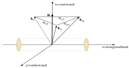
FIG. 1.: View of the interaction region for the case of 3 particle emission.

The dependence on $K$, or equivalently the rapidity $y\simeq y_{1}\simeq y_{2}$ or transverse momentum $K_{\perp}\simeq p_{\perp 1}\simeq p_{\perp 1}$, has been suppressed in (22). It is implicit in the source size parameters, $R_{l,s,o}$. Longitudinal expansion is revealed as a rapidity dependent $R_{l}$ [13] while transverse expansion may be seen through $R_{s,o}$ depending on the transverse momentum [5, 7]. For an ideal chaotic source the parameter $\lambda_{\rm 2}$ would be unity but a number of effects like a partially coherent source, long lived resonances, final state interactions and Coulomb screening effects can lead to a smaller value for $\lambda_{\rm 2}$ [10]. Finally, we would like to point out, that it is common to include a term $-2q_{\rm o}q_{\rm l}R_{\rm ol}^{2}$ for the parametrization in equation (22). We did not include this term, since we concentrate in this paper on the experimental data of NA44. The generalisation of our calculations to include this term is straight forward.

Due to low statistics it is commonplace to perform a gaussian fit of one variable only

$$C_{\rm 2}(q_{\rm inv})=1+\lambda_{\rm inv}\exp{(-q_{\rm inv}^{2}R_{\rm inv}^{2})},$$ (23)

where the invariant momentum squared is given by

$$q_{\rm inv}^{2} = {\bf q}^{2}-q_{\rm t}^{2}=q_{\rm l}^{2}+q_{\rm s}^{2}+q_{\rm o}^{2}-q_{\rm t}^{2}.$$ (24)

Here, $q_{\rm t}=E_{1}-E_{2}\simeq{\bf K}\cdot{\bf q}/E_{K}$ since $q\ll K$. Other variables, that also are used in parametrizations, are $q^{2}_{R=\tau}=q^{2}_{s}+q^{2}_{o}+q^{2}_{l}+q^{2}_{t}$ or ${\bf q}^{2}=q^{2}_{s}+q^{2}_{o}+q^{2}_{l}$. In the following we will perform an analysis in the variable $q_{inv}$ but results can be taken over by changing the sign of (for $q^{2}_{R=\tau}$) or removing (for ${\bf q}^{2}$) the last term in equations (24) and (26).

Experimental data are often analysed in the longitudinal center of mass system (LCMS) of each pair, in which $y=0$ and ${\bf K}$ is along the outward direction. In this system $q_{\rm t}=\beta_{\perp}q_{o}$, where

$$\beta_{\perp}=\frac{K_{\perp}}{\sqrt{m^{2}+K_{\perp}^{2}}},$$ (25)

is the transverse velocity in the LCMS. The LCMS–frame and the different momenta are depicted in Figure 1. The invariant relative momentum reduces to

$$q_{\rm inv}^{2} \approx q_{\rm l}^{2}+q_{\rm s}^{2}+q_{\rm o}^{2}\;(1-\beta_{\perp}^{2}).$$ (26)

We can relate $C_{\rm 2}(q_{\rm inv})$ and $C_{\rm 2}(q_{\rm l},q_{\rm s},q_{\rm o})$ if both are determined from the same data sample

$$C_{\rm 2}(q_{\rm inv})\simeq\frac{\int d^{3}q\;C_{\rm 2}(q_{\rm l},q_{\rm s},q_{\rm o})\;\delta(q_{\rm inv}^{2}-q_{\rm l}^{2}-q_{\rm s}^{2}-q_{\rm o}^{2}\;(1-\beta_{\perp}^{2}))}{\int d^{3}q\;\delta(q_{\rm inv}^{2}-q_{\rm l}^{2}-q_{\rm s}^{2}-q_{\rm o}^{2}\;(1-\beta_{\perp}^{2}))}.$$ (27)

The $\delta$–function enforces equation (24), while the numerator assures proper normalization.

In high energy nuclear collisions the sources sizes $R_{i}$, i=l,s,o, are often similar in size as in high energy pp, pA and S+Pb collisions (see [1, 2] or Tables 1 and 2). In such cases we can expand in the difference between the radii and obtain from (27)

$$C_{\rm 2}(q_{\rm inv})=1+\lambda_{\rm 2}\exp{(-q_{\rm inv}^{2}\bar{R}^{2})}\;\left[1+\frac{1}{15}\;q_{\rm inv}^{4}\;\sum_{i=l,s,o^{\prime}}(R_{i}^{2}-\bar{R}^{2})^{2}+{\cal O}(q_{\rm inv}^{6}(R_{i}^{2}-\bar{R}^{2})^{3})\right].$$ (28)

where

$$\bar{R}^{2}=\frac{1}{3}(R_{\rm l}^{2}+R_{\rm s}^{2}+{R_{\rm o^{\prime}}}^{2}),$$ (29)

is the average source size squared and

$$R_{\rm o^{\prime}}=R_{\rm o}/\sqrt{1-\beta_{\perp}^{2}}$$ (30)

is the outward radius boosted by the transverse velocity. In the limit of small $(R_{i}^{2}-R_{\rm inv}^{2})$ or small $q_{\rm inv}$ we recover $R_{\rm inv}=\bar{R}$ from a comparison of (28) and (23). Notice that $\bar{R}$ is defined such that the leading correction in (28) is second order in $(R_{i}^{2}-R_{\rm inv}^{2})$ and fourth order in $q_{\rm inv}$.

Defining the transverse and longitudinal source deformation parameters

$$\delta_{\perp} = \;\frac{R_{\rm o^{\prime}}^{2}-R_{\rm s}^{2}}{2\bar{R}^{2}}$$ (31)

$$\delta_{\rm l} = \;\frac{R_{\rm l}^{2}-\bar{R}^{2}}{2\bar{R}^{2}}$$ (32)

we can rewrite equation (28) as

$$C_{\rm 2}(q_{\rm inv})=1+\lambda_{\rm 2}\exp{(-q_{\rm inv}^{2}\bar{R}^{2})}\;\left[1+\frac{2}{5}\;q_{\rm inv}^{4}\bar{R}^{4}\;(\frac{1}{3}\;\delta_{\perp}^{2}+\delta_{\rm l}^{2})+{\cal O}(q_{\rm inv}^{6}\bar{R}^{6}\delta^{3})\right].$$ (33)

The definitions of these deformations or eccentricities are related to the deformation parameters $\beta$ and $\gamma$ of Bohr & Mottelson [8].

The deformations have a physical meaning. In many cylindrical symmetric models for sources with an emission time $\delta\tau$, one finds that $R_{o}^{2}-R_{s}^{2}=\beta_{\perp}^{2}\delta\tau^{2}$ [5, 7, 10]. Thus

$$\delta\tau^{2}=\bar{R}^{2}\;[\delta_{\perp}\;(2\beta_{\perp}^{-2}-1)+\delta_{\rm l}-1].$$ (34)

In the Bjorken 1-dimensional hydrodynamic expansion model, one finds to a good approximation that $R_{\rm l}^{2}=T\tau^{2}/\sqrt{m^{2}+K_{\perp}^{2}}$ in LCMS, where $\tau$ is the average invariant time it takes to freeze-out after the collisions and T is the temperature at freeze-out. In that case

$$\tau^{2}=\bar{R}^{2}\;\frac{p_{\perp}}{\beta_{\perp}\;T}\;(2\delta_{\rm l}\;+1)\;.$$ (35)

It may be a coincidence that the source appears to be spherical. Rephrased in terms of the deformations, we can say that the emission time is small and that the freeze-out happens when longitudinal expansion is about as large as the transverse size of the system, i.e. when the source expands in three dimensions.

We applied these results to the data samples taken in the experiment NA44 [1, 2]. Figure 2 shows in the upper left corner the results for the reaction $S+Pb\rightarrow\pi^{+}\pi^{+}X$, while the upper right corner corresponds to the reaction $p+Pb\rightarrow\pi^{+}\pi^{+}X$. In the two plots in the bottom row of Figure 2 we performed the analogous calculations for kaons. The lower left shows the results for the reaction $S+Pb\rightarrow K^{+}K^{+}X$, while lower right corresponds to the reaction $p+Pb\rightarrow K^{+}K^{+}X$. A three-parameter fit was applied to the data samples with the results listed in Table 1 and Table 2.

	$\lambda_{\rm 2}$	$R_{\rm l}\;(fm)$	$R_{\rm s}\;(fm)$	$R_{\rm o}\;(fm)$	$\langle p_{\perp}\rangle\;(MeV)$
S+Pb	0.56$\pm$0.02	4.73$\pm$0.26	4.15$\pm$0.27	4.02$\pm$0.14	150
p+Pb	0.41$\pm$0.02	2.34$\pm$0.36	2.00$\pm$0.25	1.92$\pm$0.13	150

Table 1. Parameters of the three–parameter fits to the NA44 data sample at 200 AGeV for the two–pion correlation function (from [1]).

	$\lambda_{\rm 2}$	$R_{\rm l}\;(fm)$	$R_{\rm s}\;(fm)$	$R_{\rm o}\;(fm)$	$\langle p_{\perp}\rangle\;(MeV)$
S+Pb	0.82$\pm$0.04	3.02$\pm$0.20	2.55$\pm$0.20	2.77$\pm$0.12	246
p+Pb	0.70$\pm$0.07	2.40$\pm$0.30	1.22$\pm$0.76	1.53$\pm$0.17	237

Table 2. Parameters of the three–parameter fits to the NA44 data sample at 200 AGeV for the two–kaon correlation function (from [2]).

FIG. 2.: Two–pion correlation function for the reaction $S+Pb\rightarrow\pi^{+}\pi^{+}X$ (upper left), $p+Pb\rightarrow\pi^{+}\pi^{+}X$ (upper right), $S+Pb\rightarrow K^{+}K^{+}X$ (lower left) and $p+Pb\rightarrow K^{+}K^{+}X$ (lower right). The data points are from NA44 [1, 2], the solid line is calculated using (33) and the dashed line is the 1–parameter fit (Table 5 and 6).

We would like to mention that to apply equation (27) and (33) to the three-parameter fits we have for some data samples to take into account the experimental cut–offs for low momenta. In some instances a bin size of $\delta q\sim 10$ MeV/c was applied for each momentum projection and the corresponding two other momentum projections were summed over all momenta between $0$ and $q_{\rm cut}\sim 20$ MeV/c. This prescription modifies the value of $\lambda_{\rm 2}$. For the longitudinal direction we find, for example,

$$C_{\rm 2}(q_{\rm l}) = \int_{\rm 0}^{q_{\rm cut}}\frac{dq_{\rm s}}{q_{\rm cut}}\;\int_{\rm 0}^{q_{\rm cut}}\frac{dq_{\rm o}}{q_{\rm cut}}\;C_{\rm 2}(q_{\rm l},q_{\rm s},q_{\rm o})$$ (36)

$$= 1+\lambda_{\rm 2}\exp(-q_{\rm l}^{2}R_{\rm l}^{2})\;\;\frac{\pi}{4}\;\frac{{\rm Erf}(R_{\rm s}\;q_{\rm cut})}{R_{\rm s}\;q_{\rm cut}}\;\frac{{\rm Erf}(R_{\rm o}\;q_{\rm cut})}{R_{\rm o}\;q_{\rm cut}}$$ (37)

$$\simeq 1+\lambda_{\rm 2}\exp(-q_{\rm l}^{2}R_{\rm l}^{2})\;(1-\frac{1}{3}q_{s}^{2}R_{s}^{2})((1-\frac{1}{3}q_{o}^{2}R_{o}^{2}),\quad q_{\rm cut}R_{i}\ll 1,$$ (38)

where $\rm Erf(x)$ is the error function. Corresponding equations apply to the other two directions and result in an apparent reduction of the experimentally measured $\lambda_{\rm 2}$. In the case of NA44 this prescription was not applied in the fitting procedure [9].

In Figure 2 we find reasonably good agreement between the data points (black dots), the 1–parameter fit (dashed line) and our calculation using equation (33) (solid line). The approximation (33) is in this case hardly distinguishable from the exact expression (27). The parameters used for the upper row of Figure 2 are listed in Table 3, while the parameters used for the lower row in Table 4. The parameters for the 1–parameter fit are listed in Table 5 and 6 for pions and kaons respectively.

	$R_{\rm inv}\;(fm)$	$\langle\beta_{\perp}\rangle$	$\delta_{\rm l}$	$\delta_{\perp}$
S+Pb	4.98	0.73	-0.05	0.35
p+Pb	2.41	0.73	-0.03	0.34

Table 3. Source parameters for the two–pion correlation function determined according to equations (25) and (32).

	$R_{\rm inv}\;(fm)$	$\langle\beta_{\perp}\rangle$	$\delta_{\rm l}$	$\delta_{\perp}$
S+Pb	2.90	0.44	0.04	0.18
p+Pb	1.84	0.43	0.35	0.20

Table 4. Source parameters for the two–kaon correlation function determined according to equations (25) and (32).

	$\lambda_{\rm inv}$	$R_{\rm inv}\;(fm)$
S+Pb	$0.56\pm 0.03$	$5.00\pm 0.22$
p+Pb	$0.38\pm 0.03$	$2.89\pm 0.30$

Table 5. Parameters of the 1–parameter fit to the NA44 data sample for the two–pion correlation function (from [1]).

	$\lambda_{\rm inv}$	$R_{\rm inv}\;(fm)$
S+Pb	$0.92\pm 0.08$	$3.22\pm 0.20$
p+Pb	$0.68\pm 0.06$	$1.71\pm 0.17$

Table 6. Parameters of the 1–parameter fit to the NA44 data sample for the two–kaon correlation function (from [1]).

IV Three-particle BE correlation functions

We can now apply the results of the previous sections to predict all three– and more particle correlation functions. The three-pion correlation function recently determined by NA44 [4] is especially relevant. A 1–parameter Gaussian fit was applied to the data and the radius and $\lambda$-parameter of this fit are listed in

	$\lambda$	$R_{\rm inv}\;(fm)$
S+Pb	$2.1\pm 0.4$	$2.7\pm 0.2$

Table 7. Parameters of the 1–parameter fit to the NA44 data sample for the three–pion correlation function (from [4]).

Table 7. The data was fitted in terms of the sum, $Q_{\rm 3}$, of the relative invariant momenta of the 3 particles labeled 1,2,3

$$Q_{\rm 3}^{2}=q_{\rm 12}^{2}+q_{\rm 13}^{2}+q_{\rm 23}^{2}\;.$$ (39)

The relative invariant momentum of particle i and j is hereby given as in equation (24) (see also Figure 1)

$$q_{\rm ij}^{2}={\bf q}_{\rm ij}^{2}-q_{\rm t,\,ij}^{2}\;.$$ (40)

We proceed to evaluate the three–pion correlation function $C_{3}(Q_{3})$, starting from

$$C_{\rm 3}(Q_{\rm 3})=\frac{\int d{\bf q}_{\rm 12}\;d{\bf q}_{\rm 13}\;d{\bf q}_{\rm 23}\;C_{\rm 3}({\bf q}_{\rm 12},{\bf q}_{\rm 13},{\bf q}_{\rm 23})\;\delta(Q_{\rm 3}^{2}-q_{\rm 12}^{2}-q_{\rm 13}^{2}-q_{\rm 23}^{2})\;\delta^{3}({\bf q}_{\rm 12}+{\bf q}_{\rm 13}+{\bf q}_{\rm 23})}{\int d{\bf q}_{\rm 12}\;d{\bf q}_{\rm 13}\;d{\bf q}_{\rm 23}\;\delta(Q_{\rm 3}^{2}-q_{\rm 12}^{2}-q_{\rm 13}^{2}-q_{\rm 23}^{2})\;\delta^{3}({\bf q}_{\rm 12}+{\bf q}_{\rm 13}+{\bf q}_{\rm 23})}.$$ (41)

The $\delta$–function of the sum of the relative momentum vectors assures that the 3 particles span a triangle.

As mentioned we cannot extract the phase from two-body correlation function. We shall therefore in the following assume that $F({\bf q}_{\rm ij})$ are real functions which then are known from the two-body correlation function. The three-body and any many-body correlation function is then completely given by equation (14) and (10).

At present statistics do not allow experimentalists to map out the three-body correlation function of all six variables (nine including ${\bf K}$) and we therefore reduce it according to Eq. (41).

In the case of a spherical source, we obtain from (41) and (14)

$$C_{\rm 3}(Q_{\rm 3})=1 + 3\;\lambda_{2}\;\exp(-x)\;\tilde{I}_{1}(x)+2\;\lambda_{2}^{1.5}\exp(-y)\;,$$ (42)

and for a slightly deformed source, we obtain

$$C_{\rm 3}(Q_{\rm 3})=1 + 3\;\lambda_{2}\;\exp(-x)\;\left[\tilde{I_{1}}(x)+\frac{x^{2}}{15}\;\;(\frac{1}{3}\;\delta_{\perp}^{2}+\delta_{\rm l}^{2})\;\left(4\;\tilde{I_{1}}(x)-3\;\tilde{I_{2}}(x)\right)\right]$$ (43)

$$+ 2\;\lambda_{2}^{1.5}\exp(-y)\;\left[1+\frac{y^{2}}{10}\;(\frac{1}{3}\;\delta_{\perp}^{2}+\delta_{\rm l}^{2})\right]+O(\bar{R}^{6}Q_{\rm 3}^{6}\delta^{3})\;.$$ (44)

where we used the dimensionless variable $x=\bar{R}^{2}\;Q_{\rm 3}^{2}/3$ and $y=\bar{R}^{2}\;Q_{\rm 3}^{2}/2$. $\tilde{I}_{\nu}$ is related to the standard Bessel function $I_{\nu}$

$$\tilde{I_{\nu}}(x) = (\frac{2}{x})^{\nu}\;I_{\nu}(x)=\sum_{n=0}^{\infty}\frac{(x/2)^{2n}}{n!(n+\nu)!}\;.$$ (45)

Figure 3 depicts this result, together with a 1-parameter Gaussian fit of reference [4]. A satisfactory agreement is achieved. Based on the currently available data we seem not to need any correlations beyond the two-pion correlations.

FIG. 3.: Three–pion correlation function for the reaction $S+Pb\rightarrow\pi^{+}\pi^{+}\pi^{+}X$. The data points are from NA44 [4], the solid line is calculated using (42), assuming a spherical source (no deformations) and the dashed–dotted line uses the approximation (42), allowing for deformations. Finally, the dashed line is the 1–parameter fit (Table 7).

The three-body correlation function of equation (42) or (44) is a sum of two gaussians. However, the current experimental resolution cannot resolve the last term in these expressions, since it decays with an 3/2 times larger exponential than the 3 explicit two-particle contributions and the data does not explore sufficiently small $Q_{3}$. More statistics is needed to resolve this second term which may be available in Pb+Pb collisions at the SPS or future RHIC or LHC heavy ion collisions. It is the second term that may carry a phase if, e.g., the source is asymmetric. It would therefore be most interesting to study three and more particle correlations at small $Q_{3}$ to learn more about the source.

The method can be generalized to study different aspects of the 9 dimensional phase space, if the experimental resolution should permit so, or extended to calculate any many–particle correlation function of invariant momenta.

As a last example, we would like to proceed to the 4-particle correlation function. Current data samples are not large enough to study pure 4–pion correlation functions but they do allow us to study for example two–pion–two–kaon correlation functions $C_{2\times 2}$ of equation (21). As described above the two–particle correlation studies for pions and kaons can be used to obtain the invariant radii and eccentricities for the two particles and subsequently employing equations (33) and (11) allows us to calculate $C_{\rm 2\times 2}(q_{\rm\pi\pi},q_{\rm KK})$. If the data should show any deviation from this result, we would have evidence for cross-correlations between pions and kaons.

V Coulomb Corrections

In a recent paper [14] Baym and Braun–Munzinger show that the standard use of the Gamow correction for Coulomb repulsion between pions of like charge is incorrect. The relevant length scale for the two pion wavefunction is their classical turning point in their Coulomb field, $\sim 4\alpha m_{\pi}/q^{2}\raisebox{-2.15277pt}{$\stackrel{{\scriptstyle<}}{{\sim}}$}2$ fm, for relative momenta $q\raisebox{-2.15277pt}{$\stackrel{{\scriptstyle>}}{{\sim}}$}10$ MeV/c, and not the two-pion Bohr radius, $a_{0}=2/m_{\pi}\alpha=387$ fm. Since the turning point is smaller than the typical source size in high energy nuclear collisions, the two-body interactions are insignificant as compared to those of the source. It is instead a better approximation simply to assume classical trajectories for the two charged particles in their Coulomb field, $V_{C}(r)=Z_{1}Z_{2}e^{2}/r$, once they are separated by a distance $r_{0}$ of order the source size. A good description of $\pi\pi$ and $\pi p$ correlation data from nuclear collisions at AGS was obtained with an initial separation of $r_{0}\simeq 9$ fm.

The simple model of Ref. [14] can be generalized to N particles. Energy conservation implies that the final energies, $E_{i}$, of the particles are related to the initial ones, $E_{0,i}$, by

$$\sum_{i=1}^{N}E_{i}=\sum_{i=1}^{N}E_{0,i}\,+\,\frac{N(N-1)}{2}\frac{e^{2}}{R_{0}}\,,$$ (46)

where $R_{0}$ is the N-particle equivalent of $r_{0}$ and corresponds to an average separation between the particles.

Particle number and total momentum conservation relates the final N-particle distribution $n_{N}({\bf k}_{1},...,{\bf k}_{N})$ to the initial distribution $n_{N}^{0}({\bf k}_{0,1},...,{\bf k}_{0,N})$ by

$$n_{N}({\bf k}_{1},...,{\bf k}_{N})d^{3}{\bf k}_{1}...d^{3}{\bf k}_{N}\delta(N{\bf K}-\sum_{i=1}^{N}{\bf k}_{i}) = n_{N}^{0}({\bf k}_{0,1},...,{\bf k}_{0,N})d^{3}{\bf k}_{0,1}...d^{3}{\bf k}_{0,3}\delta(N{\bf K}-\sum_{i=1}^{N}{\bf k}_{0,i})\;.$$ (47)

In terms of relative momenta, $q_{ij}=k_{i}-k_{j}$, and average four-momentum, $K=(k_{1}+...+k_{N})/N$, we find that the invariant momentum of N particles is

$$Q_{N}^{2}\equiv\frac{1}{2}\sum_{i,j=1}^{N}q_{ij}^{2}=-(NK)^{2}-(Nm)^{2}=(\sum_{i=1}^{N}E_{i})^{2}\;-\;N^{2}(m^{2}+{\bf K}^{2})\,,$$ (49)

and likewise for initial momenta. With energy conservation in the Coulomb potential, Eq. (46), we obtain

$$Q_{N}^{2}-Q_{0,N}^{2}=N^{2}(N-1)E_{K}\frac{e^{2}}{R_{0}}\,,$$ (50)

where $E_{K}=m_{\perp}\cosh Y$. Defining the corresponding N-body correlation functions analogous to (41) we obtain from Eq. (LABEL:nrel) and (50)

$$C_{N}(Q_{N})=\left(\frac{Q_{0,N}}{Q_{N}}\right)^{3N-5}C^{0}_{N}(Q_{0,N})\;.$$ (51)

The measured correlation function is thus the original one, $C^{0}_{N}(\sqrt{Q_{N}^{2}-N^{2}(N-1)E_{K}e^{2}/R_{0}})$, scaled by powers of $Q_{0,N}/Q_{N}$. In the two-body case the results reduce to those in Ref. [14]. As an numerical example, we consider the three-body correlations of NA44 in LCMS (where $Y=0$) for pions with $\langle m_{\perp}\rangle\sim 300$ MeV. Assuming $R_{0}\sim r_{0}\simeq 9$ fm the three-body invariant momentum is $Q_{3}^{2}-Q_{0,3}^{2}\simeq$ (30 MeV)². In comparison the lowest measured data point in [4] is $Q_{3}\sim 45$ MeV.

The data of NA44 [1, 2] was corrected by the Gamow factor

$$C_{2}(q_{12}) = \Gamma(q_{12})C_{2}^{0}(q_{12})\,,$$ (52)

$$\Gamma(q_{12}) = \frac{2\pi\eta}{\exp(2\pi\eta)-1}\,,\quad\eta=e^{2}m/q_{12}\;.$$ (53)

The data for the three-pion correlation function [4] was corrected ad hoc by a three-body Gamow factor $\Gamma(q_{12})\Gamma(q_{13})\Gamma(q_{23})$. Hereby Coulomb effects are overcorrected for but so are they in the two-body case at the smallest measured relative momenta . A better analysis including Coulomb effects correctly in two- and three-body correlation functions should be performed with a realistic charge distribution and not just a one parameter model as in [14] and Eq. (51).

VI Conclusion

In this paper we develop a simple procedure to predict many–particle correlation functions from Bose-Einstein interference between identical particles emitted independently from an incoherent source. Using the best available fits for the two–particle correlation function, we calculate the higher order correlation functions. Any deviation from this result should signal interesting new physics.

We apply our prescription to pion correlations. The experiment NA44 supplies a single data sample, which allows one to study two– and three–pion correlations, as well as two–pion–two–kaon correlations. We test our approach against the data for two– and three–pion correlations in terms of the total invariant momentum of the pions and find good agreement. In the case of three-pion correlations no additional three–particle correlations seem to be necessary to predict the available data. We show, how to evaluate the two-pion-two–kaon correlation function from the currently available data.

Larger data samples, like the one from the current Pb+Pb run at CERN will provide us with larger data samples and allow us a more thorough investigation of this issue. This data sample will not only improve the resolution for the three–pion correlation function, but also allow us to study 4–pion correlations.

Finally, Coulomb effects were discussed and a simple N-particle generalization of the two-particle Baym & Braun-Munzinger correction was given in terms of invariant momenta.

REFERENCES

• [1] H. Bøggild et al., NA44, Phys. Lett. B349, 386 (1995).
• [2] H. Becker et al., NA44, Z. Phys. C64, 209 (1994).
• [3] T. Alber et al., NA35, Nucl. Phys. A590, 453c (1995); Z. Phys. C66, 77 (1995); D. Ferenc et al., Nucl. Phys. A544, 531c (1992).
• [4] H. Becker et al., NA44, to be published., Janus Schmidt–Sörensen, thesis, Niels Bohr Institut (1995)
• [5] S. Chapman, J.R. Nix, and U. Heinz, Phys. Rev. C52, 2694 (1995); S. Chapman, U. Heinz and P. Scotto, Heavy Ion Physics 1,1 (1995).
• [6] S. Pratt, Phys. Rev. Lett. 53, 1219 (1984).
• [7] T. Csörgő, Phys. Lett. B347, 354 (1995); T. Csörgő and B. Lörstad, Nucl. Phys. A590, 465c (1995).
• [8] A. Bohr and B. Mottelson, Nuclear Structure, vol. II. The corresponding expressions for the parameters $R_{\rm av}$, $\beta$ and $\gamma$ in terms of $R_{\rm l},R_{\rm s},R_{\rm o^{\prime}}$ are
$\displaystyle R_{\rm av}=\frac{1}{3}\;(R_{\rm l}+R_{\rm s}+R_{\rm o^{\prime}})\;\;,\;\;\;{\beta}^{2}=\frac{8\pi}{5}\;\left(\frac{R_{\rm inv}^{2}}{R_{\rm av}^{2}}-1\right)\;\;,\;\;\;\sin\gamma=\frac{(R_{\rm s}-R_{\rm o^{\prime}})^{2}}{6\;R_{\rm inv}^{2}}\;.$ (54)
• [9] Rama Jayanti and Sanjeev U. Pandey, private communication
• [10] H. Heiselberg, Phys. Lett. B379, 27 (1996).
• [11] C.–Y. Wong, Introduction to High–Energy Heavy-Ion Collisions, World Scientific, Singapore, 1994
• [12] J. G. Cramer, Phys. Rev. C43, 2798, (1991); M. Biyajima, A. Bartl, T. Mizoguchi, O. Terazawa and N. Suzuki, Prog. Theor. Phys. 84, 931 (1990).
• [13] S.V. Akkelin and Yu.M. Sinyukov, Phys. Lett. B356 (1995) 525.
• [14] G. Baym and P. Braun-Munzinger, nucl-th/9606053, to appear in nucl. phys. A (QM’96 proceedings).