Pion-Production in Heavy-Ion Collisions at SIS energies

Abstract

We investigate the production of pions in heavy-ion collisions in the energy range of $1$ - $2$ GeV/A. The dynamics of the nucleus-nucleus collisions is described by a set of coupled transport equations of the Boltzmann-Uehling-Uhlenbeck type for baryons and mesons. Besides the $N(938)$ and the $\Delta(1232)$ we also take into account nucleon resonances up to masses of $1.9\,\,GeV/c^{2}$ as well as $\pi$-, $\eta$- and $\rho$-mesons. We study in detail the influence of the higher baryonic resonances and the $2\pi$-production channels ($NN\to NN\pi\pi$) on the pion spectra in comparison to $\pi^{-}$ data from $Ar+KCl$ collisions at $1.8$ GeV/A and $\pi^{0}$-data for $Au+Au$ at 1.0 GeV/A. We, furthermore, present a detailed comparison of differential pion angular distributions with the BEVALAC data for Ar + KCl at 1.8 GeV/A. The general agreement obtained indicates that the overall reactions dynamics is well described by our novel transport approach.

1 Introduction

Relativistic heavy-ion collisions provide a unique possibility to study nuclear matter at high density and far away from equilibrium. During the course of a heavy-ion collision at $1$ - $2$ GeV/A the nuclear matter is compressed up to $2-3$ times normal nuclear matter density $\rho_{0}$ before it expands again. The experimental probes that provide information about the compressed stage of the reaction are collective observables such as flow patterns or differential spectra of particles that have been additionally produced during the collision.

Over the last 10 years transport theories as BUU [1, 2, 3] and QMD, IQMD [4, 5, 6, 7] have been very successful in describing the reaction dynamics of heavy-ion collisions. It has been found that the experimental meson spectra can be well understood when assuming the excitation and subsequent decay of nucleon resonances during the compressed stage. Since pions couple strongly to these resonances, the differential pion spectra provide a well suited probe for the dynamics of baryonic resonances. Furthermore, due to the low production threshold, pions are produced and reabsorbed quite frequently and thus provide a signal for the whole dynamical evolution of the heavy-ion reaction. This implies in particular that a transport theoretical description of heavy-ion collisions has to reproduce the pion yields correctly before one can draw any further conclusions on more specific channels from the model. Especially for observables like dileptons the pion annihilation ($\pi^{+}\pi^{-}\to e^{+}e^{-}$) plays an important role; also the production of kaons (via $\pi N\to K\Lambda$) and $\eta$-mesons (via $\pi N\to\eta N$) is strongly influenced by the pion induced channels.

In this work we present a new implementation of the BUU-model, denoted by Coupled-Channel-BUU (CBUU), which as an extension to previous realisations in [8, 9] - or compared to the transport model IQMD [5, 6, 7] - includes all baryonic resonances up to masses of $1950$ $MeV/c^{2}$. The higher resonances are expected to contribute to the low as well as to the high momentum regimes of pion spectra via 1$\pi$ and 2$\pi$ decay channels, respectively. Apart from the pions ($\pi^{+},\,\pi^{0},\,\pi^{-}$) we now also explicitly propagate $\eta$’s and $\rho$-mesons ($\rho^{+},\,\rho^{0},\,\rho^{-}$) as mesonic degrees of freedom thus including hadronic excitations up to about 1 GeV of excitation energy. After introducing our model in section 2 and the various elastic and inelastic cross sections in section 3 we present detailed comparisons with $\pi^{-}$data taken at the BEVALAC [10] and the SIS in section 4. A summary and discussion of open problems concludes the paper in section 5.

2 The CBUU-Model

2.1 Basic Equations

In line with refs. [1, 2, 3, 11] the dynamical evolution of heavy-ion collisions or hadron-nucleus reactions below the pion-production threshold is described by a transport equation for the nucleon one-body phase-space distribution function $f_{N}(\vec{r},\vec{p},t)$,

$$\frac{\partial f(\vec{r},\,\vec{p},\,t)}{\partial t} + \left\{\frac{\vec{p}}{E}+\frac{m^{*}(\vec{r},\vec{p})}{E}\,\vec{\nabla}_{p}\,U(\vec{r},\,\vec{p})\right\}\,\vec{\nabla}_{r}f(\vec{r},\,\vec{p},\,t)$$ (1)

$$+\left\{-\frac{m^{*}(\vec{r},\vec{p})}{E}\,\vec{\nabla}_{r}U(\vec{r},\,\vec{p})\right\}\,\vec{\nabla}_{r}f(\vec{r},\,\vec{p},\,t)\,\,=\,\,I_{coll}[f(\vec{r},\,\vec{p},\,t)],$$

where $\vec{r}$ and $\vec{p}$ denote the spatial and the momentum coordinate of the nucleon, respectively, while $N$ stands for a proton ($p$) or neutron ($n$). The effective mass $m^{*}(\vec{r},\,\vec{p})$ in eq. (1) includes the nucleon restmass $m_{N}$ ($=938$ MeV/c) as well as a scalar momentum-dependent mean field potential $U(\vec{r},\,\vec{p})$,

$$m^{*}(\vec{r},\,\vec{p})=m_{N}+U(\vec{r},\,\vec{p}).$$ (2)

The nucleon quasi-particle properties then read as

$$E=\sqrt{m^{*}(\vec{r},\,\vec{p})^{2}+\vec{p}^{2}}.$$ (3)

Physically the l.h.s. of eq. (1) represents the Vlasov equation for a gas of non-interacting nucleons moving in the scalar momentum-dependent mean-field potential $U(\vec{r},\,\vec{p})$. The Vlasov equation as given above can be derived from a manifest covariant transport equation using scalar and vector self-energies depending on the four-momentum ($p^{\mu}=(E,\,\vec{p}))$ of the particles [11, 12] when neglecting the vector self-energies. Due to the quasiparticle mass-shell constraint given by (3) the scalar potential effectively depends only on the three-momentum of the nucleons as ($U(\vec{p},E(\vec{p})$).
The r.h.s. of the BUU-equation (i.e. the collision integral $I_{coll}(f(\vec{r},\,\vec{p},\,t))$ [1, 2]) describes the time evolution of $f_{N}(\vec{r},\,\vec{p},\,t)\,\,$due to two-body collisions among the nucleons. For example, the alteration in the one-body phase-space distribution function $f(\vec{r}_{1},\,\vec{p}_{1},\,t)$ due to the elastic scattering of two nucleons

$$N_{1}+N_{2}\longleftrightarrow N_{3}+N_{4},$$

with momenta ($\vec{p}_{i},\,\,i=1,..,4$) is given by [2, 3]

$$I_{coll}\left[f_{1}(\vec{r},\,\vec{p}_{1},\,t)\right] = \sum_{2,3,4}\frac{g}{(2\pi)^{3}}\,\int d^{3}p_{2}\,\int d^{3}p_{3}\,\int d\Omega_{4}\,v_{12}\,\frac{d\sigma_{12\rightarrow 34}}{d\Omega}\,\delta^{3}\left(\vec{p}_{1}+\vec{p}_{2}-\vec{p}_{3}-\vec{p}_{1}\right)$$ (4)

$$\times (f_{3}(\vec{r},\,\vec{p}_{3},\,t)\,f_{4}(\vec{r},\,\vec{p}_{4},\,t)\,\bar{f}_{1}(\vec{r},\,\vec{p}_{1},\,t)\,\bar{f}_{2}(\vec{r},\,\vec{p}_{2},\,t))$$

$$- \,\,\,f_{1}(\vec{r},\,\vec{p}_{1},\,t)\,f_{2}(\vec{r},\,\vec{p}_{2},\,t)\,\bar{f}_{3}(\vec{r},\,\vec{p}_{3},\,t)\,\bar{f}_{4}(\vec{r},\,\vec{p}_{4},\,t)),$$

where $\frac{d\sigma_{12\rightarrow 34}}{d\Omega}$ is the in-medium differential nucleon-nucleon cross section, $\bar{f}_{i}=1-f_{i}\,(i=1,..,4)$ the Pauli-blocking factors and $v_{12}$ the relative velocity between the nucleons $N_{1}$ and $N_{2}$ in their center-of-mass system. The factor $g=2$ in (4) stands for the spin degeneracy of the nucleons whereas $\sum_{2,3,4}$ stands for the sum over the isospin degrees of freedom of particles $N_{2},N_{3}$ and $N_{4}$.

For energies above the pion-production threshold one also has to account for inelastic processes such as direct meson production channels or the excitation/deexcitation of higher baryon resonances. In the CBUU-model - to be described here - we explicitly propagate the mesonic degrees of freedom $\pi$, $\eta$, $\rho$ and a scalar meson $\sigma$ that simulates correlated $2\pi$ pairs in the isospin $0$-channel. Besides the nucleon and the $\Delta(1232)$ we, furthermore, include all baryonic resonances up to a mass of $1950$ MeV/c²: i.e. $N(1440)$, $N(1520)$, $N(1535)$, $\Delta(1600)$, $\Delta(1620)$, $N(1650)$, $\Delta(1675)$, $N(1680)$, $\Delta(1700)$, $N(1720)$, $\Delta(1905)$, $\Delta(1910)$ and $\Delta(1950)$, where the resonance properties are adopted from the PDG [13].  Introducing one-body phase-space distribution functions for each particle type leads to equations similar to eq. (1) for each hadron. Since the different particle species mutually interact the integro-differential equations are coupled by the collision integrals. Schematically one can write down the set of coupled equations in the following way:

$$Df_{N} = I_{coll}[f_{N},f_{\Delta(1232)},...,f_{\Delta(1950)},f_{\pi},f_{\rho},f_{\eta},f_{\sigma}]$$

$$Df_{\Delta(1232)} = I_{coll}[f_{N},f_{\Delta(1232)},...,f_{\Delta(1950)},f_{\pi}]$$

$$... = ...$$

$$Df_{N(1535)} = I_{coll}[f_{N},f_{\Delta(1232)},...,f_{\Delta(1950)},f_{\pi},f_{\rho},f_{\eta},f_{\sigma}]$$

$$Df_{\Delta(1600)} = I_{coll}[f_{N},f_{\Delta(1232)},...,f_{\Delta(1950)},f_{\pi},f_{\rho},f_{\sigma}]$$

$$.. = ..$$

$$Df_{\Delta(1950)} = I_{coll}[f_{N},f_{\Delta(1232)},...,f_{\Delta(1950)},f_{\pi},f_{\rho},f_{\sigma}]$$

$$Df_{\pi} = I_{coll}[f_{N},f_{\Delta(1232)},...,f_{\Delta(1950)},f_{\pi},f_{\rho},f_{\sigma}]$$

$$Df_{\eta} = I_{coll}[f_{N},f_{N(1535)}]$$

$$Df_{\rho} = I_{coll}[f_{N},f_{N(1440)},...,f_{\Delta(1950)},f_{\pi}]$$ (5)

$$Df_{\sigma} = I_{coll}[f_{N},f_{N(1440)},...,f_{\Delta(1950)},f_{\pi}],$$ (6)

where $Df$ abbreviates the left side of the Vlasov-equation. The collision integrals on the r.h.s. of eq. (6) have formally the same structure as the one given in eq. (4). In addition to elastic scattering processes they now also contain all allowed transition rates. Denoting the nucleon by $N$ and the baryon resonances listed above by $R$ and $R^{\prime}$, we include explicitly the following channels:

• elastic baryon-baryon collisions

  $$NN \leftrightarrow NN$$

  $$NR \leftrightarrow NR$$

  The elastic $NN$-cross section is described within the parametrization by Cugnon [1, 14], while the cross section for elastic $NR$-scattering is evaluated by using an invariant matrix element which is extracted from the $NN$-cross section (cf. Section 3). For $NR$-scattering we also allow for a change in the resonance mass according to the corresponding distribution function (cf. Section 3).

• inelastic baryon-baryon collisions

  $$NN \leftrightarrow NR$$

  $$NR \leftrightarrow NR^{\prime}$$

  $$NN \leftrightarrow \Delta(1232)\Delta(1232)$$

  For the cross section of the reaction $NN\rightarrow N\Delta(1232)$ we use the result of the OBE-model calculation by Dimitriev and Sushkov [15]. In order to obtain the $NN\leftrightarrow NR$-cross sections for any of the higher resonances we exploit the resonance model described in more detail in Section 3, while the parametrization for the $NN\leftrightarrow\Delta(1232)\Delta(1232)$-cross section is adopted from Huber and Aichelin [16].

• inelastic baryon-meson collisions

  $$R \leftrightarrow N\pi$$

  $$R \leftrightarrow N\pi\pi$$

  $$\leftrightarrow \Delta(1232)\pi,\,N(1440)\pi,\,N\rho,\,N\sigma$$

  $$N(1535) \leftrightarrow N\eta$$

  $$NN \leftrightarrow NN\pi$$

  Besides the production and absorption in baryon-baryon collisions, baryonic resonances can also be populated in baryon-meson collisions and subsequently decay to baryons and mesons again. A detailed discussion of the respective cross sections and decay widths is given in Section 3. Here we note that the $2\pi$-decay of higher resonances is modelled via subsequent two-body decays as indicated above.

• meson-meson collisions

  $$\rho \leftrightarrow \pi\pi\,\,\,\,\,\mbox{(p-wave)}$$

  $$\sigma \leftrightarrow \pi\pi\,\,\,\,\,\mbox{(s-wave)}$$

  For the pure mesonic cross sections we use the Breit-Wigner parametrizations given in Section 3.

2.2 The Test-Particle Method

The CBUU-equations (6) are solved by means of the test-particle method, where the phase-space distribution function $f_{N}(\vec{r},\,\vec{p},\,t)\,\,$(e.g. for nucleons) is represented by a sum over $\delta$-functions:

$$f(\vec{r},\,\vec{p},\,t)=\frac{1}{N}\,\sum_{i=1}^{N\times A}\delta\left(\vec{r}-\vec{r}_{i}(t)\right)\times\delta\left(\vec{p}-\vec{p}_{i}(t)\right).$$ (7)

Here $N$ denotes the number of test-particles per nucleon while $A$ is the total number of nucleons participating in the reaction. Inserting the ansatz (7) into the CBUU-equations (6) leads to the following equations of motion for the test-particles:

$$\frac{d\vec{r}_{i}(t)}{dt} = \frac{\vec{p}}{E}+\frac{m^{*}}{E}\;\vec{\nabla}_{p}\;U(\vec{r}_{i},\,\vec{p}_{i}(t))$$

$$\frac{d\vec{p}_{i}(t)}{dt} = -\frac{m^{*}}{E}\;\vec{\nabla}_{r}\;U(\vec{r}_{i},\,\vec{p}_{i}(t)).$$ (8)

Again these equations of motion are consistent with those from a covariant transport equation [11] when using only scalar self-energies for the baryons. Thus the solution of the CBUU-equations within the test-particle method reduces to the time evolution of a system of classical point particles according to eq. (8). For the actual numerical simulation we discretize the time $t$ and integrate the equations of motion employing a predictor-corrector method [17]. We want to note that in our model pions are treated as ’free’ particles, except for the Coulomb interaction. It remains to be seen if pion selfenergies as suggested in refs. [18, 19] will alter our results.

2.3 The Collision Integrals

The collision integrals occurring in eq. (6) contain either particle-particle collisions or the decay of baryonic or mesonic resonances.
For particle-particle collisions we employ the following prescription: The test-particles collide with each other as in conventional cascade simulations with reaction probabilities that are calculated on the basis of free cross sections. The numerical implementation additionally accounts for the Pauli-blocking of the final states while the collision sequence is calculated within the Kodama algorithm [20] (cf. ref. [8]) which is an approximately covariant prescription.
The decay of a resonance, furthermore, is determined by its width $\Gamma(M)$. However, during the course of a heavy-ion collision the resonance may also decay due to collisions with other particles (eq. $NR\rightarrow NN$). This collisional broadening of a resonance is described by the collision integral for particle-particle collisions. Here we will concentrate on the numerical method used to account for the first decay mechanism. All resonances treated in the CBUU-model are allowed to decay into a two-particle final state, i.e. in every timestep of the simulation we calculate the decay probability $P$ for each resonance assuming an exponential decay law

$$P=1-e^{-\Gamma(M)/\hbar\gamma\Delta t},$$ (9)

where $\Delta t$ is the time step size of our calculation, $\Gamma(M)$ is the energy-dependent width of the resonance and $\gamma$ the Lorentz factor related to the velocity of the resonance with respect to the calculational frame. We then decide by means of a Monte Carlo algorithm if the resonance may decay in the actual timestep and to which final state it may go. If the chosen final state contains a nucleon, which e.g. is Pauli-blocked, we reject the resonance decay.

3 Explicit numerical Implementations

3.1 Nuclear Mean-Field Potentials

Particles propagating inside nuclear matter are exposed to the mean-field potential generated by all other particles. From Dirac-phenomenological optical-model calculations [11, 21] it is known that elastic nucleon-nucleus scattering data can only be described when using proper momentum-dependent potentials. Here we employ the momentum-dependent mean-field potential proposed by Welke et al. [22], i.e.

$$U^{nr}(\vec{r},\,\vec{p})=A\frac{\rho}{\rho_{0}}+B\frac{\rho}{\rho_{0}}^{\tau}+2\frac{C}{\rho_{0}}\int d^{3}p^{\prime}\frac{f(\vec{r},\vec{p^{\prime}})}{1+\left(\frac{\vec{p}-\vec{p^{\prime}}}{\Lambda}\right)^{2}}.$$ (10)

As an extension of the momentum-independent Skyrme type potentials for nuclear matter [3, 22] the parametrization (10) has no manifest Lorentz-properties. However, definite Lorentz-properties are required for a transport model at relativistic energies. To achieve this goal we evaluate the non-relativistic mean-field potential $U^{nr}$ in the local rest frame (LRF) of nuclear matter which is defined by the frame of reference with vanishing local vector baryon current ($\vec{j}(r,t)=\vec{0}$). Discarding vector potentials in the LRF we then equate the expressions for the single-particle energies using the non-relativistic potential $U^{nr}$ and the scalar potential $U$ by

$$\sqrt{p^{2}+m^{2}}+U^{nr}(\vec{r},\,\vec{p})=\sqrt{p^{2}+\left(m+U\left(\vec{r},\,\vec{p}\right)\right)^{2}}.$$ (11)

Eq. (11) now allows to extract the scalar mean-field potential $U(\vec{r},\,\vec{p})$ which we will use throughout our calculations for the baryons. Due to the relativistic dispersion relation for the quasiparticle (11) the scalar potential $U(\vec{r},\,\vec{p})$ now has definite Lorentz-properties contrary to $U^{nr}$. This enables us to guarantee energy conservation in each two-body collision and in resonance decays (eq. $N_{1}+N_{2}\rightarrow N_{3}+N_{4}$) as

$$E_{1}+E_{2} = E_{3}+E_{4}$$

$$\sqrt{\vec{p}_{1}^{2}+m_{1}^{*\,2}}+\sqrt{\vec{p}_{2}^{2}+m_{2}^{*\,2}} = \sqrt{\vec{p}_{3}^{2}+m_{3}^{*\,2}}+\sqrt{\vec{p}_{4}^{2}+m_{4}^{*\,2}}.$$ (12)

Since the collision integrals (6) are evaluated in the center-of-mass system of the colliding particles or in the restframe of the decaying resonance, while the testparticle equations of motion are generally integrated in the center-of-mass system of the heavy-ion reaction, energy conservation is not a priori fulfilled when employing non-relativistic potentials without definite properties under Lorentz transformations.
For our calculations we will use a (momentum-dependent) equation of state (EOS) for nuclear matter with an incompressibility of K = 250 MeV ( A = -29.253 MeV, B = 57.248 MeV, C = -63.516 MeV, $\tau$ = 1.760, $\Lambda$ = 2.13 1/fm.)  The actual calculation of the mean-field potential according to eq. (10), however, is too involved for practical purposes since one has to perform double integrations for the momentum-dependent part of $U^{nr}(\vec{r},\ \vec{p})$. We thus determine the potentials within the Local Thomas-Fermi approximation, where the integral over the phase-space distribution function in (10) can be performed analytically [22]. With

$$f(\vec{r},\vec{p})=\frac{4}{(2\pi\hbar)^{3}}\,\Theta(p_{F}-p),$$

where the factor $4$ stems from the sumation over spin and isospin, the integral for the momentum-dependent part of the potential $U^{nr}$ reads:

$$\int d^{3}p^{\prime}\frac{f(\vec{r},\vec{p^{\prime}})}{1+\left(\frac{\vec{p}-\vec{p^{\prime}}}{\Lambda}\right)^{2}}= \frac{4}{(2\pi\hbar)^{3}}\,\pi\Lambda^{3}\left[\frac{p_{F}^{2}+\Lambda^{2}-p^{2}}{2p\Lambda}ln\frac{\left(p+p_{F}\right)^{2}+\Lambda^{2}}{\left(p-p_{F}\right)^{2}+\Lambda^{2}}\right.$$

$$\left.+\frac{2p_{F}}{\Lambda}-2\left[arctan\frac{p+p_{F}}{\Lambda}-arctan\frac{p-p_{F}}{\Lambda}\right]\right].$$

We employ a smeared baryon density [3] when evaluating expression (3.1) rather than that obtained directly from the test-particle distribution in order to avoid unphysical statistical fluctuations in the density and in the mean-field potentials.

3.2 The Coulomb Potential

Charged baryons and mesons are additionally exposed to the Coulomb potential $V_{c}(\vec{r})$ generated by all charged particles. Since in our present approach mesons are propagated as free particles with respect to the nuclear mean-field, the Coulomb force

$$\vec{F}_{c}\left(\vec{r}\right)=-q\,\vec{\nabla}_{r}V_{c}\left(\vec{r}\right)$$ (14)

is the only force acting on a meson with charge $q$. For charged baryons the force $F_{c}$ (14) represents an additional term in the equations of motion (8). The Coulomb potential $V_{c}\left(\vec{r}\right)$ is obtained by solving the Poisson-equation by means of the Alternating-Direction Implicit Iterative (ADI-)algorithm [23].

3.3 Resonance Properties and Decay Widths

Within the CBUU-approach the resonances are treated as ”on-shell” particles with respect to their propagation and the evaluation of cross sections. To account for their ”off-shell” behaviour, we distribute the resonance masses according to a Lorentzian distribution function (see sec. (3.5)), which is determined by the mean resonance masses $M_{R}$ and the total and partial decay widths $\Gamma_{R}$ at mass $M_{R}$. For the baryonic resonances these explicit parameters are given in table 1. For the $\rho$-meson we use a mean mass $M_{R}=770$ MeV/c² and for the decay width at resonance $\Gamma_{R}=118$ MeV. The corresponding values for the $\sigma$-meson are $M_{R}=800$ MeV/c² and $\Gamma_{R}=800$ MeV.

			branching ratio [%]
resonance	$\overline{\left|\mbox{$\cal M$}^{2}\right|}/16\pi$	$\Gamma_{R}$			N $\pi\pi$
	[$mb\,GeV^{2}$]	[$MeV$]	N $\pi$	N $\eta$	$\Delta\pi$	N $\rho$	N $(\pi\pi)_{s-wave}^{I=0}$	$N(1440)\pi$
$\Delta$(1232)	-	120	100	0	0	0	0	0
$N$(1440)	14	350	65	0	25	0	10	0
$N$(1520)	4	120	55	0	25	15	5	0
$N$(1535)	8, 40	203	50	45	0	2	0	3
$\Delta$(1600)	68	350	15	0	75	0	0	10
$\Delta$(1620)	68	150	30	0	60	10	0	0
$N$(1650)	4	150	80	0	7	5	4	4
$\Delta$(1675)	68	150	45	0	55	0	0	0
$N$(1680)	4	130	70	0	10	5	15	0
$\Delta$(1700)	7	300	15	0	55	30	0	0
$N$(1720)	4	150	20	0	0	80	0	0
$\Delta$(1905)	7	350	15	0	25	60	0	0
$\Delta$(1910)	68	250	50	0	50	0	0	0
$\Delta$(1950)	14	300	75	0	25	0	0	0

Table 1: Decay widths and decay channels for the baryonic resonances. The data for these channels are taken from [13] and [25] in case of the $N(1535)$. The second column contains the averaged matrix-elements for the production of the baryon resonances in nucleon-nucleon collisions (cf. sec. 3.5.2).

In the following we list the parametrizations used for the decay widths $\Gamma(M)$.

• $1\pi$-decay width for the $\Delta(1232)$
  For the $\Delta(1232)$-decay we adopt the parametrization given by Koch et al. [24]

  $$\Gamma_{Moniz}(q)=\Gamma_{R}\frac{M_{\Delta}}{M}\left(\frac{q}{q_{r}}\right)^{3}\left(\frac{q_{r}^{2}+\delta^{2}}{q^{2}+\delta^{2}}\right)^{2},$$ (15)

  where $M$ is the actual mass of the $\Delta(1232)$ and $M_{\Delta}=1232$ MeV/c². $q$ and $q_{r}$ are the pion three-momenta in the restframe of the resonance with mass $M$ and $M_{\Delta}$, respectively. The parameter $\delta$ in the cutoff function has a value $\delta=0.3$ GeV/c².

• $1\pi$-decay width for the higher baryon resonances
  The $1\pi/\eta$-decay widths for the higher baryon resonances are given by

  $$\Gamma(q)=\Gamma_{R}\left(\frac{q}{q_{r}}\right)^{2l+1}\left(\frac{q_{r}^{2}+\delta^{2}}{q^{2}+\delta^{2}}\right)^{l+1},$$ (16)

  where $l$ is the angular momentum of the emitted pion or $\eta$ and $q$ and $q_{r}$ are the momenta of the pion or $\eta$ in the restframe of the decaying resonance as defined above. In this case, we use

  $$\delta^{2}=(M_{R}-M_{N}-m_{\pi})^{2}+\frac{\Gamma_{R}^{2}}{4}$$ (17)

• $2\pi$-decay width for baryon resonances
  The $2\pi$-decay of the higher baryon resonances is described by a two-step process. First, a higher lying baryonic resonance decays into a $\Delta(1232)$ or $N(1440)$ and a pion or into a nucleon and $\rho$- or $\sigma$-meson. The new resonances then propagate through the nuclear medium and eventually decay into a nucleon and pion or a nucleon and two pions

  $$R\rightarrow r\,b\rightarrow N\,\pi\,\pi.$$ (18)

  Here R denotes the higher baryonic resonances, r stands for a $\Delta(1232)$, $N(1440)$, $\rho$ or $\sigma$ and b is a nucleon or pion, respectively. Due to the fact that a further resonance appears in the first step of reaction (18) one has to integrate the corresponding distribution function over the mass $\mu$ of the intermediate resonance $r$ in order to obtain the $2\pi$-decay width

  $$\Gamma_{R\to r\,b}(M) = \frac{P_{2\pi}}{M}\int_{0}^{M-m_{b}}d\mu\,p_{f}\,\frac{2}{\pi}\frac{\mu^{2}\,\Gamma_{r,tot}(\mu)}{(\mu^{2}-m_{r}^{2})^{2}+\mu^{2}\,\Gamma_{r,tot}^{2}(\mu)}$$ (19)

  $$\times\left(\frac{\left(M_{R}-M_{N}-2m_{\pi}\right)^{2}+\delta^{2}}{\left(M-M_{N}-2m_{\pi}\right)^{2}+\delta^{2}}\right)^{2},$$

  where $P_{2\pi}$ is the branching ratio for the $2\pi$-decay of the baryonic resonance $R$ and $p_{f}$ denotes the momentum of $r$ and $b$ in the restframe of $R$. Since the integral in eq. (19) for high resonance masses $M$ is proportional to $M$, we introduce a cutoff function to avoid $\Gamma_{R\to r\,a}(M)$ to diverge for high masses. The parameter $\delta$ used is 0.3 GeV.

• decay width for meson resonances
  The decay width of the meson resonances is parametrized similarly to that of the $\Delta(1232)$,

  $$\Gamma(M)=\Gamma_{r}\frac{M_{r}}{M}\left(\frac{q}{q_{r}}\right)^{2J_{r}+1}\frac{q_{r}^{2}+\delta^{2}}{q^{2}+\delta^{2}},$$ (20)

  where $M_{r}$ and $M$ are the mean mass and the actual mass of the meson resonance. $q$ and $q_{r}$ are defined as in eq. (15) while $J_{r}$ is the spin of the resonance and $\Gamma_{r}$ the decay width for a resonance with mass $M_{r}$. For the parameter $\delta$ in the cutoff function we use again $\delta$ = 0.3 GeV.

3.4 Meson-Baryon Cross Sections

In order to describe meson-baryon scattering in the framework of our resonance picture we use a Breit-Wigner formulation for the cross sections (eq. $\pi N\rightarrow\pi N$)

$$\sigma_{ab\rightarrow R\rightarrow cd}=\frac{2J_{R}+1}{(2S_{a}+1)(2S_{b}+1)}\,\frac{4\pi}{p_{i}^{2}}\frac{s\,\Gamma_{R\rightarrow ab}\,\Gamma_{R\rightarrow cd}}{(s-M_{R}^{2})^{2}+s\,\Gamma_{tot}^{2}}.$$ (21)

In eq. (21) $ab$ and $cd$ denote the baryon and the meson in the final and initial state of the reaction and $R$ is the intermediate baryon resonance. $J_{R}$, $S_{a}$ and $S_{b}$ are the spins of the baryon resonance and the particles in the initial state of the reaction.
The solid line in fig. 1 shows the total $\pi^{-}-p$-cross section within our model in comparison to the experimental data from [26]. To calculate this cross section we replace the partial widths $\Gamma_{R\to cd}$ in eq. (21) by the total widths of the baryonic resonances and sum up the contributions from all resonances. The dashed, the dotted and the dash-dotted lines in fig. 1 show the contributions from the $\Delta(1232)$, the $N(1440)$ and the $N(1535)$ separately.

Figure 1: The calculated total $\pi^{-}-p$-cross section in comparison to the data from [26] is given by the solid line. The dashed, the dotted and the dashed-dotted lines show the contributions from the $\Delta(1232)$, $N(1440)$ and $N(1535)$, respectively.

Figure 2: The solid line shows the cross section for the reaction $\pi^{-}p\rightarrow\eta n$ as obtained from eq. (21). The data are taken from [26].

In fig. 2 we display the resulting cross section for the $\pi^{-}p\rightarrow\eta n$ reaction. Here only the $N(1535)$ contributes since this is the only baryonic resonance that couples to the $\eta$ within our model space (cf. table 1). Both cross sections are obviously well described up to $p_{\pi}\approx$ 1.0 GeV.
Eq. (21) is also used to determine the cross sections for $\sigma$- and $\rho$-production in $\pi-\pi$-collisions weighting with the corresponding spins of the mesonic resonances and the pions in the initial state of the reaction.

3.5 Inelastic Baryon-Baryon Cross Sections

In this section we describe the concepts and parametrizations used to implement the cross sections for resonance, pion and $\eta$ production in the CBUU-model.

3.5.1 The $NN\to N\Delta(1232)$ Cross Section

For the $NN\to N\Delta(1232)$ cross section we employ the result of the OBE-model calculation by Dimitriev and Sushkov [15] using $u$- and $t$-channel Born-diagrams. The parameters of the model ($NN\pi$-, $N\Delta(1232)\pi$-coupling constant and a parameter in the $\pi$-formfactor) are chosen to reproduce the experimental $pp\to N\Delta^{++}$ cross section. For the implementation of this cross section into the CBUU-model we replace the parametrization for the $\Delta(1232)$-width given in [15] by the Moniz parametrization (15). An example for the resulting mass and angular differential cross sections for an invariant energy of $2.31$ GeV is given in fig. 3 in comparison to the experimental data [15]. The cross sections for the other isospin channels follow from the $pp\to n\Delta^{++}$ cross section by applying isospin symmetry.

Figure 3: Comparison of the $pp\to n\Delta(1232)$ angular and mass differential cross section at an invariant energy of $2.31$ GeV (solid lines) with the experimental data [15] (filled circles).

3.5.2 The $NN\to NR$ Cross Section

In order to obtain the production cross sections for the higher baryon resonances in nucelon-nucelon collisions we fit the corresponding matrix-elements to available data for $\eta$-, $1\pi$-, $\rho$- and $2\pi$-production in nucleon-nucleon reactions. Therefore we assume that the $\eta$-, $1\pi$-, $\rho$- and $2\pi$-production in nucleon-nucleon collisions above the $\Delta(1232)$ excitation proceed only through these resonances via subsequent two-step processes. The $\eta$, single pion and $\rho$ production are described by the creation of a baryonic resonance in a nucleon-nucelon collision and its subsequent decay into $\eta$, pion or $\rho$

$$NN\to NR\to NN\pi/\eta/\rho.$$ (22)

We assume that the $2\pi$-production in nucleon-nucleon collisions proceeds either through the excitation of two $\Delta(1232)$ and their subsequent decay into a nucleon and a pion or through the excitation of higher lying baryonic resonances and their subsequent decay into a nucleon and two pions (see section (3.3)).

• The general expression for the cross section
  For the derivation of the cross section we assume that in a collision of two nucleons $a+b\to R+c$ a baryonic resonance $R$ and a nucleon $c$ are produced. Then resonance $R$ decays into a two-body final state$R\to de$. Assuming spinless particles the invariant matrix element is given by

  $$\mbox{$\cal M$}_{ab\rightarrow cde}=\mbox{$\cal M$}_{ab\rightarrow Re}\,P_{R}\,\mbox{$\cal M$}_{R\rightarrow cd},$$ (23)

  where $P_{R}$ is the propagator of the intermediate baryonic resonance $R$ and ${\cal M}_{ab\rightarrow Re}$ and ${\cal M}_{R\rightarrow cd}$ are the matrix elements for the reactions $a+b\to R+e$ and $R\to c+d$, respectively. We start from the general expression for the cross section

  $$d\sigma_{ab\rightarrow cde} = \frac{(2\pi)^{4}}{4\,p_{i}\,\sqrt{s}}\,\delta^{4}(p_{a}+p_{b}-p_{c}-p_{d}-p_{e})\overline{\left|\mbox{$\cal M$}_{ab\rightarrow cde}\right|^{2}}$$ (24)

  $$\times\frac{d^{3}p_{c}}{(2\pi)^{3}\,2E_{c}}\frac{d^{3}p_{d}}{(2\pi)^{3}\,2E_{d}}\frac{d^{3}p_{e}}{(2\pi)^{3}\,2E_{e}},$$

  where $\sqrt{s}$ is the invariant energy of the particles in the initial state and $p_{i}$ is their CMS momentum. $\overline{\left|\mbox{$\cal M$}_{ab\rightarrow cde}\right|^{2}}$ is the square of the invariant matrix element averaged over the spin of particles $a$ and $b$ and summed over the spins of the particles in the final state of the reaction. Assuming that the square of the matrix element factorizes as

  $$\overline{\left|\mbox{$\cal M$}_{ab\rightarrow cde}\right|^{2}}=\overline{\left|\mbox{$\cal M$}_{ab\rightarrow Re}\right|^{2}}\left|P_{R}\right|^{2}\overline{\left|\mbox{$\cal M$}_{R\rightarrow cd}\right|^{2}},$$ (25)

  we obtain for the cross section as a function of the resonance mass $\mu$

  $$\frac{d\sigma_{ab\to Re\to cde}}{d\mu}=\sigma_{ab\to Re}(\mu)\,\frac{2}{\pi}\,\frac{\mu^{2}\,\Gamma_{R\to cd}}{(\mu^{2}-M_{R}^{2})^{2}+\mu^{2}\,\Gamma_{tot}^{2}}.$$ (26)

  Here, $\sigma_{ab\to Re}(\mu)$ is the cross section for producing a baryonic resonance $R$ with a fixed mass $\mu$

  $$\sigma_{ab\to Re}(\mu)=\frac{1}{64\,\pi^{2}\,s\,p_{i}}\int d\Omega\,p_{f}\overline{\left|\mbox{$\cal M$}_{ab->Re}(\mu)\right|^{2}},$$ (27)

  with $p_{f}$ and $p_{i}$ denoting the CMS momenta of the particles in the final and initial state of the reaction $a+b\to R+e$, respectively, while $s$ is the squared invariant energy of this reaction. When evaluating the production cross sections for the higher baryonic resonances we assume $\overline{\left|\mbox{$\cal M$}_{ab->Re}(\mu)\right|^{2}}$ to be constant for all baryonic resonances except for the $\Delta(1232)$ (cf. section (3.5.1)).
  

• $\eta$-production cross section
  Since in our model only the $N(1535)$ couples to the $\eta$-meson, we obtain the cross section for $\eta$-production in nucleon-nucleon collisions from eq. (26) by using the $N(1535)$ as the intermediate baryonic resonance and regarding $NN\eta$ as the final state $cde$. The unknown squares of the matrix elements $\overline{\left|\mbox{$\cal M$}_{ab->Re}\right|^{2}}$ are obtained by fitting the available experimental data for $\eta$-production in nucleon-nucleon collisions. The matrix element for $N(1535)$ production in proton-proton collisions then gives

  $$\overline{\left|\mbox{$\cal M$}_{p\,p\to p\,N^{+}(1535)}\right|^{2}}=16\pi\times 8{\rm\,mb\,GeV^{2}}.$$ (28)

  The result of this fit for the reaction $pp\rightarrow pp\eta$ is displayed in fig. 4 in comparison to the data [27, 26].

  

  Figure 4: Cross section for the reaction $pp\to pp\eta$ obtained from the resonance model using the matrix element given in eq. (28) (solid line) in comparison to the experimental data [27, 26].

  It is known from [27] that the cross section for $\eta$-production in proton-neutron collisions is about a factor $5$ larger than that for proton-proton collisions. Consequently we use

  $$\overline{\left|\mbox{$\cal M$}_{p\,n\to p\,N(1535)}\right|^{2}}=\overline{\left|\mbox{$\cal M$}_{p\,n\to n\,N^{+}(1535)}\right|^{2}}=16\pi\times 40{\rm\,mb\,GeV^{2}}.$$ (29)

• $1\pi$-production cross section
  In order to evaluate the $1\pi$-production cross sections in nucleon-nucleon collisions we sum up the contributions from all resonances contributing to a specific channel incoherently. For $\Delta(1232)$-production we use the cross section given in sec. (3.5.1) and for the other baryonic resonances we use eq. (26) integrated over the resonance mass $\mu$ with $a$ and $b$ denoting the two nucleons in the initial state and $c$, $d$ and $e$ the $NN\pi$ final state. Introducing the proper isospin coefficients we obtain

  $$\sigma_{p\,p\to p\,p\,\pi^{0}} = \frac{2}{3}\sigma_{3/2}+\frac{1}{3}\sigma_{1/2}$$ (30)

  $$\sigma_{p\,p\to p\,n\,\pi^{+}} = \frac{10}{3}\sigma_{3/2}+\frac{2}{3}\sigma_{1/2}$$ (31)

  $$\sigma_{p\,n\to p\,p\,\pi^{-}} = \frac{1}{3}\sigma_{3/2}+\frac{1}{3}\sigma_{1/2}$$ (32)

  $$\sigma_{p\,n\to p\,n\,\pi^{0}} = \frac{4}{3}\sigma_{3/2}+\frac{1}{3}\sigma_{1/2},$$ (33)

  with

  $$\sigma_{3/2} = \sum_{I_{R}=\frac{3}{2}}p\,p\to p\,R^{+}=\sigma_{p\,p\to p\,\Delta^{+}(1232)}\,$$ (34)

  $$+\frac{1}{4}\frac{\overline{\left|\cal M\right|^{2}}}{16\pi\,p_{i}\,s}\,\int_{M_{N}+m_{\pi}}^{\sqrt{s}-M_{N}}\,d\mu\,p_{f}\times\sum_{R\neq\Delta(1232)\atop I_{R}=\frac{3}{2}}\frac{\mu^{2}\,\Gamma_{R\to N\,\pi}(\mu)}{\left(\mu^{2}-M_{R}^{2}\right)^{2}+\mu^{2}\,\Gamma_{R,tot}^{2}(\mu)}\quad$$

  and

  $$\sigma_{1/2} = \sum_{I_{R}=\frac{1}{2}}p\,p\to p\,R^{+}$$ (35)

  $$= \frac{\overline{\left|\cal M\right|^{2}}}{16\pi\,p_{i}\,s}\,\int_{M_{N}+m_{\pi}}^{\sqrt{s}-M_{N}}\,d\mu\,p_{f}\sum_{R\atop I_{R}=\frac{1}{2}}\frac{\mu^{2}\,\Gamma_{R\to N\,\pi}(\mu)}{\left(\mu^{2}-M_{R}^{2}\right)^{2}+\mu^{2}\,\Gamma_{R,tot}^{2}(\mu)}.$$

  There is no explicit factor $\Gamma_{N\pi}$ in the contribution of the $\Delta(1232)$ to $\sigma_{3/2}$ (34) because it decays with $100\%$ probability into a nucleon and a pion.
  

• $\rho$-production cross section
  The invariant matrix-elements for the production of baryon resonances which can decay into a nucleon and a $\rho$ (cf. table 1) are obtained by a fit to the experimental data for the reaction

  $$pp\to pp\rho^{0}.$$ (36)

  Similar to eq. (30) we write the $\rho^{0}$-production cross section as a sum of contributions of $I=3/2$- and $I=1/2$-resonances,

  $$\sigma_{pp\to pp\rho^{0}}=\frac{2}{3}\sigma_{3/2}+\frac{1}{3}\sigma_{1/2},$$ (37)

  where $\sigma_{3/2}$ and $\sigma_{1/2}$ are defined as in eqs. (34) and (35), while the sum extends only over resonances with a non-vanishing branching ratio for the decay into a nucleon and a $\rho$. The resulting matrix-elements are quoted in the second column of table 1. The corresponding $\rho^{0}$-production cross section is shown in fig. 5 in comparison to the experimental data [26].

  

  Figure 5: Cross section for the reaction $pp\to pp\rho^{0}$ obtained from the resonance model using the matrix elements given in table 1 (solid line) in comparison to the experimental data [26].

• The $2\pi$-production cross section
  As already stated in sec. (3.3) the $2\pi$-production cross section in nucleon-nucleon collisions is described via the excitation of higher lying baryonic resonances and their subsequent decay into a nucleon and two pions according to the branching ratios given in table 1 and the corresponding decay widths:

  $$1.\mbox{ }NN\to NR\to N\Delta(1232)\pi \to NN\pi\pi$$ (38)

  $$2.\mbox{ }NN\to NR\to NN(1440)\pi \to NN\pi\pi$$ (39)

  $$3.\mbox{ }NN\to NR\to NN\rho \to NN\pi\pi$$ (40)

  $$4.\mbox{ }NN\to NR\to NN\sigma \to NN\pi\pi.$$ (41)

  Here $R$ stands for the higher lying baryon resonances. In addition to these processes we take into account the $2\pi$-production via the excitation of two $\Delta(1232)$,

  $$NN\to\Delta(1232)\Delta(1232)\to NN\pi\pi,$$ (42)

  adopting the cross sections from ref. [16]. For the description of the $2\pi$-production cross section in nucleon-nucleon collisions we define $\sigma^{i}_{3/2}$ and $\sigma^{i}_{1/2}$ ($i=1,..,4$) similarly to eqs. (34) and (35) replacing $\Gamma_{R\to N\pi}$ by the corresponding decay width $\Gamma_{i}$ ($i=1,..,4$) responsible for the second step of the reactions (38) to (41). The cross sections then read

  $$\sigma_{NN\to NN\pi\pi}=\sum_{i=1}^{4}n_{i}\sigma^{i}_{1/2}+\sum_{i=1}^{4}d_{i}\sigma^{i}_{3/2}+\sigma_{NN\to\Delta(1232)\Delta(1232)\to NN\pi\pi},$$ (43)

  where the $n_{i}$ and $d_{i}$ are the products of the isospin coefficients for the three steps of the reactions (38) - (41). The corresponding factors are listed in table 2.

  	$pp\to pp\pi^{+}\pi^{-}$	$pp\to pp\pi^{0}\pi^{0}$	$pp\to pn\pi^{+}\pi^{0}$	$pn\to pn\pi^{+}\pi^{-}$	$pp\to pp\pi^{-}\pi^{0}$
  $n_{1}$	$5/9$	$2/9$	$2/9$	$5/9$	$2/9$
  $n_{2}$	$4/9$	$1/9$	$4/9$	$4/9$	$4/9$
  $n_{3}$	$1/3$	$0$	$2/3$	$1/3$	$2/3$
  $n_{4}$	$2/3$	$1/3$	$0$	$2/3$	$0$
  $d_{1}$	$26/45$	$2/45$	$22/9$	$52/45$	$17/45$
  $d_{2}$	$2/9$	$2/9$	$14/9$	$4/9$	$5/9$
  $d_{3}$	$2/3$	$0$	$10/3$	$2/3$	$1/3$
  $d_{4}$	0	0	0	0	0

  Table 2: The products of the isospin coeficients for the three steps of the reactions (38) - (41) for those isospin channels where experimental data are available.

Using the matrix elements already determined by the fits to the $\eta$- and $\rho$-production data we now adjust the unknown matrix elements $\overline{\left|\mbox{$\cal M$}_{NN\to NR}\right|^{2}}$ to reproduce the cross sections for $1\pi$- and $2\pi$-production in nucleon-nucleon collisions.

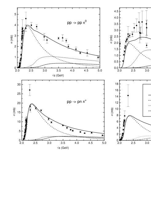
Figure 6: The fitted $1\pi$-production cross sections (solid line) for different isospin channels in comparison to the data [26]; contributions from the $\Delta(1232)$ (dashed), the isospin 1/2 resonances (dotted), the higher isospin 3/2 resonances (dashed-dotted).

The resulting $1\pi$-cross sections are shown in fig. 6 (solid line), where the contributions from the $\Delta(1232)$ (dashed line), the sum of all contributions from the isospin-$1/2$ resonances (dotted line) and the sum of all higher isospin-$3/2$ resonances (dash-dotted line) are displayed separately. Evidently the pion-cross sections are fitted in our resonance model reasonably well up to invariant energies of $5$ GeV.
In fig. 7 we plot the resulting $2\pi$-production cross section (43) for the isospin channels where experimental data are available [26]. As in case of the $1\pi$-production channels the $2\pi$-data can be reproduced well within our multi-resonance model using the matrix elements given in table 1.

Figure 7: Cross sections for $2\pi$-production in nucleon-nucleon collisions for different isospin channels obtained within the simple resonance model in comparison to the experimental data [26].

3.5.3 The $NR\to NN$ Cross Section

The cross sections for the reaction $NR\to NN$, where $R$ stands for the $\Delta(1232)$ as well as a higher baryonic resonances, are given by an expression corresponding to eq. (24) for a two-body final state. For the matrix elements involved we adopt those from the OBE-model of Dimitriev [15] for the $\Delta(1232)$ and those from the simple resonance model (sec. (3.5.2)) in case of higher baryon resonances. Thus, in comparison to previous implementations of the BUU-model [28, 29] we do not have to employ a detailed balance prescription to deduce the $NR\to NN$-cross section, since the matrix elements are known as a function of the invariant energy and the resonance mass.

3.5.4 The $NR\to NR^{\prime}$-Cross Section

For the collisions of a nucleon and a resonance $R$ leading to a nucleon and a different resonance $R^{\prime}$ we use for all resonances (including the $\Delta(1232)$) the average of the matrix elements obtained for the reactions $NN\to NR$ and $NN\to NR^{\prime}$. In analogy to eq. (26) this leads to the following expression

$$\sigma_{NR\to NR^{\prime}\atop R\neq R^{\prime}}= I\,\frac{0.5(\left|\mbox{$\cal M$}_{NN\to NR}\right|^{2}+\left|\mbox{$\cal M$}_{NN\to NR^{\prime}}\right|^{2})\,2\,(2J_{R^{\prime}}+1)}{16\,\pi\,p_{i}\,s}$$

$$\times\int\,d\mu\,p_{f}\frac{2}{\pi}\,\frac{\mu^{2}\,\Gamma_{R^{\prime}}(\mu)}{\left(\mu^{2}-M_{R^{\prime}}^{2}\right)^{2}+\mu^{2}\,\Gamma_{R^{\prime}}^{2}(\mu)},$$

where $I$ accounts for the proper isospin coefficients (cf. table 3) and $J_{R}^{\prime}$ stands for the spin of the resonance in the final channel.

I $N^{+}$ $N^{+}$ $N^{+}$ $N^{+}$ 1 $N^{+}$ $N^{0}$ $N^{+}$ $N^{0}$ 1/2 $N^{+}$ $N^{+}$ $N^{0}$ $\Delta^{++}$ 3/4 $N^{+}$ $N^{+}$ $N^{+}$ $\Delta^{+}$ 1/4 $N^{+}$ $N^{0}$ $N^{+}$ $\Delta^{0}$ 1/4 $N^{+}$ $\Delta^{++}$ $N^{+}$ $\Delta^{++}$ 1 $N^{+}$ $\Delta^{+}$ $N^{0}$ $\Delta^{++}$ 3/8 $N^{+}$ $\Delta^{+}$ $N^{+}$ $\Delta^{+}$ 5/8 $N^{+}$ $\Delta^{0}$ $N^{+}$ $\Delta^{0}$ 1/2 $N^{+}$ $\Delta^{-}$ $N^{+}$ $\Delta^{-}$ 5/8

Table 3: Isospin coefficients $I$ for baryon-baryon collisions. $N$ and $\Delta$ represent isospin $1/2$ and isospin $3/2$ particles, respectively. The isospin channels not listed explicitely are determined by assuming isospin symmetry.

3.5.5 The $NN\to NN\pi$-Cross Section

The $NN\to NR$-cross sections are determined by fitting the experimental data for $1\pi$-production in nucleon-nucleon collisions above the $\Delta(1232)$. As compared to the data the resulting $1\pi$-cross sections are slightly too low just above the $\pi$-production threshold (cf. fig. 8).

Figure 8: The $1\pi$-production cross section taking into account only the contributions due to the decay of baryonic resonances (dashed line) and the total cross sections obtained by adding the direct pion production in nucleon-nucleon collisions (solid line) in comparison to the experimental data [26].

In order to compensate for this deficit we attribute the difference between the data and the cross sections obtained from the resonance model to the cross section for direct (s-wave) $\pi$-production in nucleon-nucleon collisions ($NN\to NN\pi$). The resulting difference (s-wave) cross section can be fitted by the expression

$$\sigma_{N\,N\to N\,N\,\pi}(x)=A\,x^{n_{1}}\,e^{-\left(a\,x^{n_{2}}+b\,x\right)},$$ (45)

with

$$x=\frac{\sqrt{s}-2M_{N}-m_{\pi}}{5\,{\rm GeV}},$$

using the parameters given in table 4.

channel A [mb] a b $n_{1}$ $n_{2}$ $p\quad p\to p\quad p\quad\pi^{0}$ 61.3 1.52 2.50 6.18 3.48 $p\quad p\to p\quad n\quad\pi^{+}$ 122.6 1.52 2.50 6.18 3.48 $p\quad n\to p\quad p\quad\pi^{-}$ 24.9 3.30 0.85 1.93 0.002 $p\quad n\to p\quad n\quad\pi^{0}$ 7.25 0.88 0 2.31 3.64

Table 4: Parameters obtained for the direct $\pi$-production cross section $\sigma_{N\,N\to N\,N\,\pi}$ (eq. (45)).

Now adding $\sigma_{N\,N\to N\,N\,\pi}$ incoherently to the $1\pi$-production cross section from the baryon resonance decays then yields the total cross section depicted in fig. 8 by the solid line which now also gives a fit at threshold.

3.5.6 The $NN\pi\to NN$-Rate

Assuming that the invariant matrix element for the reaction $N_{1}+N_{2}\to N_{3}+N_{4}+\pi$ depends only on the invariant energy one can write the cross section $\sigma_{N_{1}\,N_{2}\to N_{3}\,N_{4}\,\pi}$ (see sec. (3.5.5)) in the following form [13]

$$\sigma_{N_{1}N_{2}\to N_{3}N_{4}\pi}(\sqrt{s})=\frac{S_{N_{1},N_{2}}}{64\,(2\,\pi)^{3}\,p_{i}\,\sqrt{s}^{3}}\,\left|\mbox{$\cal M$}_{N_{1}\,N_{2}\to N_{3}\,N_{4}\,\pi}(\sqrt{s})\right|^{2}\,\int dm_{34}^{2}\,dm_{3\pi}^{2}.$$ (46)

Here $S_{N_{1},N_{2}}$ is the symmetry factor for $N_{1}$ and $N_{2}$, $p_{i}$ is the CMS momentum of the nucleons in the initial state and

$$m_{34}^{2}=(p_{3}+p_{4})^{2},\mbox{ }m_{3\pi}^{2}=(p_{3}+p_{\pi})^{2}.$$

The transition rate for a pion being absorbed by $N_{3}$ and $N_{4}$ is given by

$$W_{fi}=(2\pi)^{4}\,\frac{\delta^{4}\left(p_{N,1}+p_{N,2}-p_{N,3}-p_{N,4}-p_{\pi}\right)\,|\mbox{$\cal M$}|^{2}}{V^{5}}\quad,$$ (47)

where the normalization volume $V$ contains $2E$ particles [30]. Multiplying this equation with the phase-space factors for the two nucleons ($N_{1}$, $N_{2}$) in the final state and taking into account that the pion reacts with two nucleons from the surrounding nuclear medium gives

$$\Gamma_{\pi N_{3}N_{4}\to N_{1}N_{2}} = S_{N_{1},N_{2}}\,\frac{p_{f}}{4\,\pi\,\sqrt{s}}|\mbox{$\cal M$}|^{2}\,\frac{1}{2\,E_{\pi}}\,\frac{\rho_{N,3}}{2E_{N,3}}\,\frac{\rho_{N,4}}{2E_{N,4}},$$ (48)

where $\rho_{N,3}$ and $\rho_{N,4}$ are the corresponding local neutron or proton densities.

3.6 Elastic Baryon-Baryon Cross Sections

For the elastic nucleon-nucleon cross section we use the conventional Cugnon parametrization [1, 14]

$$\sigma_{NN\to NN}=\left(\frac{35}{1+\frac{\sqrt{s}-2M_{N}}{{\rm GeV}}}+20\right)\,{\rm mb}.$$ (49)

The cross sections for nucleon-resonance scattering (with the same baryonic resonance in the initial and final channel) are determined in the following way: assuming an isotropic angular dependence for (49) we fix the matrix element squared by

$$\left|\mbox{$\cal M$}_{NN\to NN}\right|^{2}=16\,\pi\,s\left(\frac{35}{1+\frac{\sqrt{s}-2M_{N}}{{\rm GeV}}}+20\right)\,{\rm mb}.$$ (50)

Now inserting (50) in eq. (26) we obtain for the elastic nucleon-baryon scattering cross section

$$\sigma_{NR\to NR}=\frac{\left|\mbox{$\cal M$}_{NN\to NN}\right|^{2}}{16\,\pi\,p_{i}\,s}\int\,d\mu\,p_{f}\frac{2}{\pi}\,\frac{\mu^{2}\,\Gamma_{R}(\mu)}{\left(\mu^{2}-M_{R}^{2}\right)^{2}+\mu^{2}\,\Gamma_{R}^{2}(\mu)}.$$ (51)

We note that the cross section (51) in addition to elastic scattering also allows for a change in mass of the resonance in the scattering process.

4 Results for Nucleus-Nucleus Collisions and Comparison to Data

As described above the current implementation of the CBUU model takes into account baryonic resonances up to masses of $1.95$ $GeV/c^{2}$ for the first time. Hence, we start our discussion with an analysis of the effects of these resonances on the resulting pion spectra. Since the higher baryon resonances decay ultimately into a nucleon and one pion or into a nucleon and two pions (cf. sec. (3.5.2)) we expect the contributions from those resonances to show up in the low energy as well as in the high energy regime of the pion spectra. An enhancement of the pion yield in the low energy regime is expected due to the $2\pi$-channels ($NN\to\Delta(1232)\Delta(1232)\to NN\pi\pi,\,NN\to NR\to N\pi\pi$, sec. (3.5.2)). Pions produced via the decay of two $\Delta(1232)$, that are excited simultaneously in a nucleon-nucleon collisions, or via the $2\pi$-decay of the higher resonances have a lower momentum than those stemming from the reaction $NN\to NR\to NN\pi$. Thus we expect an enhancement of the low energy pion yield. On the other hand, once a higher baryon resonance is excited and subsequently decays into a nucleon and a single pion, this pion will have a higher momentum in the restframe of the resonance than those emitted in $\Delta(1232)$-decays.

In fig. 9 we show the effect of the $2\pi$-channels on the low energy regime of the pion spectra. Fig. 9 displays the total $\pi$-multiplicity weighted with $1/p_{T}$ as a function of the pion transverse momentum $p_{T}$ for a central $Au+Au$ reaction at $1.5$ AGeV. The solid line represents the result of a full CBUU-calculation and the dashed line is obtained by switching off the $2\pi$-channels. This is done by neglecting the cross section $NN\to\Delta(1232)\Delta(1232)$ as well as that for the time reversed reaction. The effect of the $2\pi$-decay of the higher resonances is eliminated by allowing only the decay into a nucleon and a single pion, i. e. ($\Gamma_{1\pi}/\Gamma_{tot}=1$ and $\Gamma_{2\pi}=0$). In addition the matrix elements for resonance production in nucleon-nucleon scattering have been refitted in order to guarantee the correct description of the $1\pi$-production cross sections in nucleon-nucleon collisions. The resulting value for the matrix element squared in the latter case is

$$\overline{\left|\mbox{$\cal M$}_{N,N\to N,R}\right|^{2}}=16\pi\times 9\,{\rm mb\,GeV^{2}}.$$

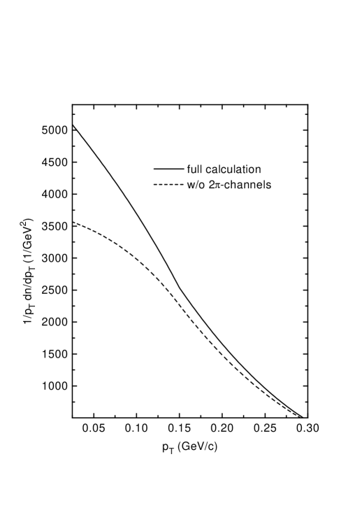
Figure 9: Total pion multiplicity weighted with $1/p_{T}$ as a function of the transverse momentum $p_{T}$ for a central ($b=0.0$ fm) $Au+Au$ collision at $1.5$ GeV/A. The solid line shows the result of the full CBUU-calculation and the dashed line corresponds to the result when omitting the $2\pi$-production channels as described in the text.

As can be seen from fig. 9 at 1.5 GeV/A the $2\pi$-channels increase the pion yield at low $p_{T}$ by $20-25\%$. The effect vanishes already at a transverse momentum of $0.25$ to $0.3$ GeV/c. For beam energies about 1.0 GeV/A we find that this effect is reduced to $\approx 10\%$.

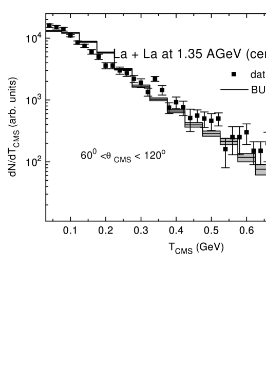
Figure 10: The $\pi^{-}$-multiplicity for central $La+La$ collisions at $1.35$ GeV/A as a function of the center of mass pion kinetic energy for $80^{o}\leq\Theta_{CMS}\leq 120^{o}$. The solid histogram displays the result of the calculation while the shaded areas indicate the statistical error of the calculation. The data (squares) are taken from [31].

Figure 11: The $\pi^{-}$-multiplicity for central $La+La$ collisions at $1.35$ AGeV as a function of the center-of-mass pion kinetic energy. Solid line: CBUU-calculation, dotted line: fraction of pions stemming from $\Delta(1232)$-, $\rho$-, $\sigma$-decay or from direct pion production in nucleon-nucleon collisions; dashed line: fraction of pions originating from decays of higher baryonic resonances. Histograms: fraction of pions from specific resonance decays: solid $N(1440)$, dotted $N(1535)$, dash-dotted $N(1520)$ and dashed $\Delta(1600)$.

After investigating the effect of the $2\pi$-channels on the $\pi$-spectra we now discuss the impact of the higher baryonic resonances at high pion kinetic energies. In this respect we display in fig. 10 the $\pi^{-}$-multiplicity in central $La+La$ collisions at 1.35 AGeV as a function of the center-of-mass kinetic energy of the pions at $80^{o}\leq\Theta_{CMS}\leq 120^{o}$ obtained from a CBUU-calculation in comparison to the experimental data from [31]. We are able to reproduce the experimental spectrum; especially the slope at high pion energies ($T_{CMS}\geq 0.5$ GeV) is described well by the calculation. That this slope is influenced significantly by the higher lying resonances is shown in fig. 11, where we display the calculated pion multiplicity for a central $La+La$ collision at 1.35 GeV/A as a function of the center-of-mass pion kinetic energy. The upper solid line corresponds to the full calculation while the dotted line displays final pions stemming from direct pion production in nucleon-nucleon collisions or from $\Delta(1232)$-, $\rho$- or $\sigma$-decay. The dashed line corresponds to the sum of the final pions stemming from the decay of higher baryonic resonances; the histograms show individually the contributions from single resonances to the pion yield: $N(1440$ (solid line), $N(1535)$ dashed line, $N(1520)$ dash-dotted line and $\Delta(1600)$ dashed line. The sum of the contributions from higher resonances for low kinetic energies is in the order of $10-20\%$ while the yield above $T_{CMS}\approx 0.6$ GeV is fully dominated by pions originating from the decay of higher resonances.

We now turn to a comparison of our calculations to the data on $\pi^{-}$-production in $Ar$ + $KCL$ collisions at $1.8$ GeV/A obtained at the BEVALAC. All data shown in the following are taken from ref. [10]. In the experimental analysis a central and a minimum bias event class have been used. In order to be able to relate the CBUU-results to the experimental events we determine these event classes by comparing to the $\frac{d\sigma}{dp_{T}}$-spectrum. The inclusive cross section is obtained by the integration of the multiplicities $n(b)$ over the impact parameter $b$ via

$$\frac{d\sigma}{dp_{T}}=2\pi\,\int_{0}^{\infty}\frac{dn(b)}{dp_{T}}bdb.$$ (52)

In order to identify the ”central event” class we thus integrate up to a maximal impact parameter $b_{max}$, which we determine by fitting the data. Fig. 12 shows these cross sections as a function of the transverse pion momentum $p_{T}$ from the CBUU-model for $b_{max}$ from $1.6$ to $2.3$ $fm$. In this $b_{max}$-regime one can see that the shape of the calculated spectrum does not depend on the events used; one only observes a shift of the spectrum in magnitude when including more events. Since the integrated spectrum is reproduced well for $b_{max}=2.1$ $fm$, we will use events with $b\leq 2.1fm$ for the comparison of the CBUU-calculations with the data.

Figure 12: The $\pi^{-}$-cross section for central event classes as a function of the transverse momentum $p_{T}$. The squares indicate the data from [10] while the lines show the result of a CBUU-calculation with different $b_{max}$ : solid line $b_{max}=2.1$ fm , dashed line $b_{max}=1.7$ fm, dotted line $b_{max}=1.9$ fm, dash-dotted line $b_{max}=2.3$ fm.

Figure 13: The differential cross section $E\frac{d\sigma}{dE}$ for the central event class ($b_{max}=2.1fm$) as a function of the pion-kinetic energy. The squares indicate the data from [10] and the solid line corresponds to the calculation.

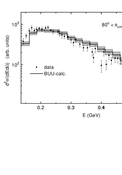
Figure 14: The double differential $\pi^{-}$-cross section for the central event class as a function of the pion-energy. The squares represent the data, while the solid line corresponds to the result of the CBUU-calculation. The shaded areas indicate the statistical errors of the calculation.

From fig. 12 we see that the spectral form of the data is described well over the whole momentum range except for the transverse momenta between $0.3$ and $0.55$ GeV/c where the data are overestimated. This overall agreement is also found when looking at $E\frac{d\sigma}{dE}$ as a function of the pion kinetic energy in the CMS (cf. fig. 13), although we find that the distribution resulting from the calculation seems to be shifted by $\approx 25$ MeV to higher energies. In fig. 14, furthermore, we show a double differential spectrum where the data are indicated by the squares and the solid histrogram corresponds to the result of the CBUU-calculation obtained by scaling the original calculation in units $mb/GeV/sr$ by a factor $1.9$. Again we observe a good agreement for the form of the spectrum, although again the calculation seems to overestimate the data between 0.3 and 0.5 GeV.

After convincing ourselves that the CBUU-model reproduces the spectral form for the $\pi^{-}$-distributions rather well we now turn to differential pion angular distributions. In fig. 15 we display $\frac{dN}{dcos\theta}$ for the inclusive $\pi^{-}$-yield, i.e. integrating eq. (52) up to $\infty$ (top), and for the central event class (bottom) in comparison to the data [10]. The circles represent the data while the squares indicate the results of the calculation. The solid lines are fits to the calculations employing the functional form [10]

$$\frac{dN}{dcos\theta}=const\times(1.0+a\,cos^{2}\theta).$$ (53)

Figure 15: The number of pions as a function of $cos\theta$ in the CMS for minimum bias (top) and central (bottom) events. The data are represented by the circles and the results of the CBUU-calculations are given by the squares. The solid lines represent fits of the form (53) to the CBUU-calculations.

For both event classes the data are reproduced remarkably well. When considering the minimum bias event class we find for the anisotropy parameter $a\approx 1.03$, while $a$ is reduced to $\approx 0.51$ when looking only at central events. As stated in [10] this decrease of anisotropy - when going from minimum bias to central events - can be understood as an effect of the centrality of the heavy-ion collision because for minimum bias events semi-peripheral and peripheral collisions are weighted stronger than central collisions (c.f. eq. (52)). Pions produced in semi-peripheral and peripheral collsions are more likely to originate from first chance $NN\to N\Delta\to NN\pi$ collisions than those produced in central collisions. Thus the anisotropy introduced in these first chance collisions prevails over the more isotropic pion distributions originating from central collisions. This line of argument is supported by the fact that the anisotropy coefficient is reduced to half of its value when considering only central collisions (see. bottom of fig. 15). In central heavy-ion collisions a high density regime is formed where pions and baryonic resonances are produced and absorbed repeatedly. Thus, pions from central collisions result mainly from multi-step processes and hence are emitted more isotropically than pions from peripheral collisions.
Finally, we look (for the central event class) at the energy dependence of the anisotropy parameter $a$ assuming as in [10]

$$\sigma(E)\sim 1+a(E)\,cos^{2}\theta.$$ (54)

Figure 16: The anisotropy parameter $a$ (see text) as a function of the pion-kinetic energy for the central event class. The circles represent the data and the squares indicate the result obtained by fitting the CBUU-results in the regime $0.0\leq cos\theta\leq 0.9$ by $const(1+a(E)cos^{2}\theta)$ for fixed pion kinetic energy.

In fig. 16 we show $a(E)$ as a function of the pion-kinetic energy. The result obained from the CBUU-model is depicted by the squares while the circles indicate the data. The overall functional form of the data is reproduced by the calculation except for the pronounced peak for pion kinetic energies of $0.25$ to $0.35$ GeV. The CBUU-model also shows the increase in anisotropy for energies up to $0.3$ GeV from zero to an $a(E)$ of $\approx 1.0$. Above these energies we observe a slight decrease of the anisotropy coefficient $a(E)$.
In fig. 17 we finally compare our calculations to the more recent data on $\pi^{0}$-production in $Au+Au$ collisions at 1.0 AGeV from the TAPS-collaboration. The solid histogram shows the result of our calculation, while the shaded areas indicate the statistical error of the calculation. The squares represent the data form [32, 33]. Here we find that our calculation is in good agreement with the experimental data, only slightly overestimating the spectrum in the region of $p_{T}\approx 0.2$ GeV/c. In comparison to earlier calculations within the BUU-model of ref. [34] the low $p_{T}$-behaviour of the pion-spectrum has improved. In addition we are now able to reproduce the high $p_{T}$-data while the earlier calculation overestimated the high $p_{T}$-spectrum. The results obtained by Bass et al. within the IQMD-model [7] are $\approx$ 20 % higher than ours in the low $p_{T}$-region, while both calculations are well in line for the other $p_{T}$-regions.

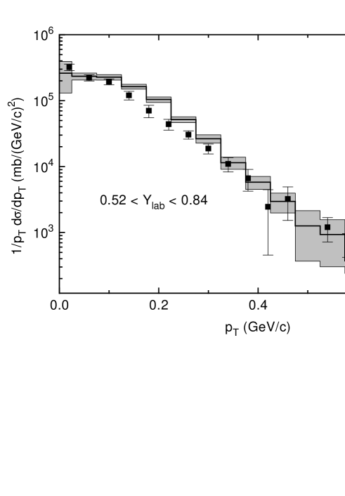
Figure 17: Cross section for $\pi^{0}$-production in $Au+Au$ collisions at 1.0 GeV/A for $0.52\leq Y_{lab}\leq 0.84$ as a function of the pion transverse momentum $p_{T}$. The solid histogram displays the result of the CBUU-calculation, while the shaded areas indicate the statistical error of the calculation. The data TAPS-data are represented by the squares. These data from ref. [32] have been renormalized by a factor $0.6$ determined by a recent new analysis [33].

5 Summary

In this paper we have presented a new implementation of the CBUU-transport-model for the description of relativistic heavy-ion collisions up to energies of about $2$ GeV/A including baryonic resonances up to masses of $1.95$ $GeV/c^{2}$ as well as $\pi,\eta$ and $\rho$ mesons. In addition to earlier implementations we also include 2$\pi$ production channels via $NN\rightarrow\Delta\Delta\rightarrow NN\pi\pi$ and the 2$\pi$-decays of higher baryon resonances. The inclusive 1$\pi$ and 2$\pi$ cross sections from nucleon-nucleon collisions are found to be well reproduced within our multi-resonance approach.

A detailed analysis of nucleus-nucleus collisions from 1 - 2 GeV/A shows that the 2$\pi$ production channels increase the pion yield essentially in the region of low transverse momenta $p_{T}$ while the one pion decays of the higher baryon resonances are dominating the high $p_{T}$ or energetic part of the pion spectrum. Thus the energetic part of the pion spectrum directly reflects the abundancy of higher baryon resonances in the compressed stage of the nucleus-nucleus collision.

In comparison to the $Ar+KCl$-data at $1.8$ AGeV for $\pi^{-}$-production obtained at the BEVALAC we found an overall agreement of the spectral $\pi^{-}$-distributions from the CBUU-model with the data except for the low $p_{T}$-regime where the data are slightly underestimated. In comparing our calculations with the $\pi^{0}$-data of the TAPS-collaboration for Au + Au at 1 GeV/A we find that the CBUU-model is in good agreement with the experimental spectrum, except for transverse momenta of $\approx 0.2$ GeV/c, where the data are overestimated. Furthermore, we have shown that the experimentally observed angular anisotropies for pions are reproduced well and can be understood in the framework of the multi-resonance picture.

References

- [1] G. F. Bertsch and S. Das Gupta: Phys. Rep. 160 (1988) 189.
- [2] W. Cassing, K. Niita and S. J. Wang: Z. Phys. A331 (1988) 439
- [3] W. Cassing, V. Metag, U. Mosel and K. Niita: Phys. Rep 188 (1990) 363
- [4] J. Aichelin: Phys. Rep. 202 (1991) 233
- [5] St. A. Bass: GSI-93-13 Report (1993)
- [6] St. A. Bass, C. Hartnack, H. Stöcker and W. Greiner: Phys. Rev. Lett. 71 (1993) 1144
- [7] St. A. Bass, C. Hartnack, H. Stöcker and W. Greiner: Phys. Rev. C51 (1995) 3343
- [8] Gy. Wolf, W. Cassing, U. Mosel and M. Schäfer: Nucl. Phys. A517 (1990) 615
- [9] Gy. Wolf, W. Cassing and U. Mosel: Nucl. Phys. A552 (1993) 549
- [10] R. Stock: Phys. Rep. 135 (1986) 259
- [11] K. Weber, B. Blättel, W. Cassing, H.-C. Dönges, V. Koch, A. Lang and U. Mosel: Nucl. Phys. A539 (1992) 713; K. Weber, B. Blättel, W. Cassing, H.-C. Dönges, A. Lang, T. Maruyama and U. Mosel: Nucl. Phys. A552 (1993) 571
- [12] T. Maruyama, W. Cassing, U. Mosel, S. Teis and K. Weber: Nucl. Phys. A573 (1994) 653
- [13] Review of Particle Properties: Phys. Rev. D50 (1994)
- [14] J. Cugnon, D. Kinet and J. Vandermeulen: Nucl. Phys. A379 (1982) 553
- [15] V. Dimitriev and O. Sushkov: Nucl. Phys. A459 (1986) 503
- [16] S. Huber and J. Aichelin: Nucl. Phys. A573 (1994) 587
- [17] J. Stoer and R. Burlirsch: vol. 1, Springer-Verlag, Berlin, (1978)
- [18] W. Ehehalt, W. Cassing, A. Engel, U. Mosel and Gy. Wolf: Phys. Lett. B298 (1993) 31
- [19] L. Xiong, C.M. Ko and V. Koch: Phys. Rev. C47 (1993) 788
- [20] T. Kodama, S. B. Duarte, K.C. Chung, R. Donangelo and R. A. M. S. Nazareth: Phys. Rev. C29 (1984) 2146
- [21] L.G. Arnold and B.C. Clark: Phys. Rev. C19 (1979) 917
- [22] G. Welke, M. Prakash, T.T.S. Kuo and S. Das Gupta: Phys. Rev C38, (1988) 2101
- [23] R. S. Varga: Matrix iterative analysis, Prentice Hall 1962
- [24] J. H. Koch, E.J. Moniz and N. Ohtsuka: Ann. Phys. 154 (1084) 99
- [25] B. Krusche, J. Ahrens, G. Anton, R. Beck, M. Fuchs, A.R. Gabler, F. H rtner, S. Hall, P. Harty, S. Hlavac, D. MacGregor, C. McGeorge, V. Metag, R. Owens, J. Peise, M. Röbig-Landau, A. Schubert, R. S. Simon, H. Ströher and V. Tries: Phys. Rev. Lett. 74 (1995) 3736
- [26] Baldini et al.: Landolt-B rnstein vol. 12, Springer, Berlin (1987)
- [27] E. Chiavassa, G. Dellacasa, N. De Marco, C. De Oliveira Martins, M. Gallio, P. Guaita, A. Musso, A. Piccotti, E. Scomparin, E. Vercellin, J. M. Durand, G. Milleret and C. Wilkin: Phys. Lett. B337 (1994) 192
- [28] A. Engel, W. Cassing, U. Mosel, M. Schäfer and Gy. Wolf: Nucl. Phys. A572 (1994) 657
- [29] P. Danielewicz and G. F. Bertsch: Nucl. Phys. A533 (1991) 712
- [30] F. Halzen and A. D. Martin: John Wiley & Sons, New York (1984)
- [31] G. Odynec, J. Bartke, S. I. Chase, J. W. harris, H. G. Pugh, G. Rai, W. Rauch, L. S. Schroeder, L. Teitelbaum, M. Tincknell, R. Stock, R. Rnfordt, R. Brockmann, A. Sandoval, H. Str bele, K. L. Wolf and J. P. Sulivan: Proceedings of the High Energy Heavy Ion Study, LBL (1987) 215
- [32] O. Schwalb, M. Pfeiffer, F.-D. Berg, M. Franke, W. Kühn, V. Metag, M. Notheisen, R. Novotny, J. Ritman, M. E. Röbig-Landau, J. P. Alard, N. Basitid, N. Brummund, P. Dupieux, A. Gobbi, N. Herrmann, H. D. Hildenbrand, S. Hlavac, S. C. Jeong, H. Löhner, G. Montarou, W. Neubert, A. E. Raschke, R. S. Simon, U. Sodan, M. Sumera, K. Teh, C. B. Venema, H. W. Wilscheit, J. P. Wessels, T. Wienhold and D. Wohlfart: Phys. Lett. B321 (1994) 20
- [33] V. Metag: private communication; The data from ref. [32] have been renormalized by a factor determined by a recent new analysis.
- [34] U. Mosel: Nucl. Phys. A583 (1995) 29c