Microscopic Calculation of the ${}^{4}{\rm He}$ System

1 Introduction

The ${}^{4}{\rm He}$ atomic nucleus is one of the best studied nuclei, both experimentally and theoretically, as summarized in the recent $A=4$ compilation [1]. Besides the many textbook examples of the gross structure, there are subtle points, usually neglected, which yield large effects. Most of these effects are only qualitatively and in most cases never quantitatively explained. None of the existing calculations aims at a complete understanding of the many features of ${}^{4}{\rm He}$ no wonder in view of the many different phenomena studied so far [1]. With the recent compilation [1] and the comprehensive $R$-matrix analysis [2] of a large amount of scattering data below 10 MeV, a microscopic calculation for the ${}^{4}{\rm He}$ system in this energy range is most needed for. The difficulties arise already for the total energy of the ground state. In most cases, parameters of the effective nucleon-nucleon potential are modified in such a way as to reproduce that energy or the threshold energies, but seldom both simultaneously. Calculations using effective potentials, however, allow to reproduce only some features, while failing in others. Therefore it remains unclear if the failure is due to the deficiencies of the potential or of the model itself. Only calculations employing realistic nucleon-nucleon potentials without any adjustable parameters can help to answer this question. Such calculations, however, are very complicated and very time consuming, no matter what type of approach is chosen. For realistic potentials, calculating the ground state energy is already a major effort and only three-body forces allow to reproduce that energy within a few keV in Greens-function Monte-Carlo calculations [3]. The next open question is the structure of the first excited state, the $0^{+}$ state just between the ${}^{3}{\rm H}-p$ and the ${}^{3}{\rm He}-n$ thresholds, considered frequently to be a breathing mode, which is reasonably narrow. In calculations this state quite often turns out to be bound (see e.g. [4]). On the experimental side this state shows a peculiar behaviour, indicating a very broad structure in $\alpha-\alpha$ breakup [5]. The $R$-matrix analysis [2] indicates the possible origin of this feature. All the other resonances do not exihibit any narrow structure, but turn out to have a decay width of the order of MeV [1, 6], which makes their location rather arbitrary. On the other side there is such an amount of scattering data, that phase shift analyses are possible, especially for proton-triton and ${}^{3}{\rm He}$-neutron scattering. The $R$-matrix analysis [2] connects all the possible reaction channels simultaneously, thus giving the most complete description and allowing to interpolate to every desired energy or reaction. Since the number of parameters in this analysis is in the order of one hundred, however, an unrestricted fitting procedure is not possible and some physical input is needed, which will be discussed below.

The aim of this paper is to show that with present-day computers, a rather unrestricted calculation using realistic nucleon-nucleon potentials, like the Bonn potential [7], is feasible and yields essentially all known experimental features. What we consider most surprising is the close agreement between the $R$-matrix analysis, which has as input only data in the ${}^{4}{\rm He}$ system, and the refined Resonating Group calculation [8], which has as input only a realistic nucleon-nucleon potential without any adjustable parameters.

We organize the paper in the following way: the next chapter contains a brief review of the Resonating Group Model (RGM) and the model space used for the calculation, where we want to point out the essential differences with existing calculations. After that, we review the $R$-matrix analysis with special emphasis on all restrictions employed in the fitting of the data. The next chapter is devoted to a detailed description of the calculation for the ground state of ${}^{4}{\rm He}$. Then we start with a comparison of the RGM and $R$-matrix results for the various partial waves. Finally we compare selected data with the results of the $R$-matrix analysis and the RGM-calculation, and give a brief outlook.

2 Resonating Group Model and the Model Space for ${}^{4}{\rm\bf He}$

The Resonating Group Model in its various modifications [8, 9, 10] is a suitable method to calculate the scattering of composite objects. In this case the main technical problem lies in the evaluation of the many-body matrix elements. In order to facilitate the calculation of the orbital matrix elements, however, all radial dependencies have to be of Gaussian form, since only then proper antisymmetrization for the translationally invariant wave function is feasible. Therefore also the potential has to be given in terms of Gaussian functions. In this work we use the $r$-space version of the Bonn-potential [7] expressed in Gaussian functions [11]. All further reference to the Bonn-potential is indeed a reference to this Gaussian version. Powerful techniques have been developed to achieve the analytic calculation of the individual matrix elements [8, 10] . Even with these techniques, calculations are usually far from trivial, hence most calculations are restricted to single channel problems, neglecting e.g. effects of the tensor-force, and/or use rather simple effective potentials. Since the calculation of the orbital matrix elements is the most time consuming part, symmetries of the orbital wave function are exploited as far as possible [8] . For simple (central or non-central) potentials, single harmonic oscillator wave functions yield already a good description of the ground state wave function of the lightest nuclei (see e.g. [4]). For a realistic $N-N$ potential this is no longer the case, because of the strongly repulsive shortranged core of the potential, which suppresses the wave function for small internucleon distances. In many cases even a node occurs in the wave function at small distances. In terms of Gaussians this means that more than one Gaussian width parameter is needed to describe even the simplest wave function. Furthermore, the tensor force plays a crucial role. Let us explain the situation for the simplest nucleus, the deuteron: For an effective $N-N$ interaction a single $S$-wave binds the deuteron already; for a reasonable radius of the wave function a linear combination of two Gaussian functions is enough (see [4, 8]). For a realistic potential only a superposition of $S$- and $D$-waves yields a bound deuteron, with at least 3 Gaussians on the $S$-wave and two on the $D$-wave for the Bonn potential [7] (see Appendix A for the detailed wave function). For other potentials, e.g. [12], we find the same behaviour. In the ${}^{4}{\rm He}$ system we have three two-fragment channels, the triton-proton, the ${}^{3}{\rm He}$-neutron, and the deuteron-deuteron channel. For the latter, the $D$-wave admixture in the wave function leads to an additional coupling of internal angular momenta of 2 to the relative orbital angular momentum. These couplings lead to very complicated wave functions for the composite system and increase the computing time neccessary by orders of magnitude. Since we allow for orbital angular momenta inside the deuteron, we treat the ${}^{4}{\rm He}$ system essentially as a four nucleon system, i.e. we consider it as a four cluster problem in the framework of the RGM. Also the triton-proton channel is treated as a four-cluster problem, because we need internal $D$-waves to bind the triton. To get a reasonable binding energy, we need $D$-waves on all internal coordinates, thus leading to a three-cluster description of the triton. Here we need three different Gaussian width parameters on both internal coordinates. To lower the binding energy even more, we allow for a second set of width parameters for all components of the wave function containing at least one $D$-wave. Some details are given in Appendix A. Since in ${}^{3}{\rm He}$ only a neutron is exchanged against a proton compared to the triton, the structure of the wave function is identical, with just modified sets of Gaussian width parameters, given in Appendix A.

Figure 1: Angular momentum structure of the ${}^{3}{\rm He}$ wave function.

Allowing for all possible combinations of $l_{1}\leq 2$ and $l_{2}\leq 2$ (see fig. 1) that can contribute to $J^{\pi}=1/2^{+}$, we get a total of 23 combinations. The total binding energy and the individal contributions of kinetic and potential energy compare favourably well with the results of Carlson [3] (see table 1). This wave function, however, is too complicated to be used in a full-fledged scattering calculation. Therefore we restricted the triton wave function to the dominant terms. These are all three spin-isospin combinations with $l_{1}=l_{2}=0$ and furthermore all combinations with the proton-neutron subsystem having spin=1 and pairs $l_{1},l_{2}$ coupled to $l_{3}$ are $[1,1]2$, $[2,0]2$, $[0,2]2$, $[2,2]0$, $[2,2]1$, and $[2,2]2$. This restricted wave function consists of only 10 combinations and yields only about 70 keV less binding energy than the full wave function (see table 1), but saves large amounts of computing time. In test cases we convinced ourselves that this reduction of the wave function of our physical channels has only minor effects on the ${}^{4}{\rm He}$ results. Also for ${}^{3}{\rm He}$ we use the similarly restricted wave function.

Table 1: Comparison of triton results with other calculations and ${}^{3}{\rm He}$ results

calculation	energy	$\big{<}V\big{>}$	$\big{<}-\frac{\hbar^{2}}{2m}\Delta\big{>}$	$\sqrt{\big{<}r^{2}_{i}\big{>}}$	$P_{l_{tot}=2}$
	[MeV]	[MeV]	[MeV]	[fm]	[%]
Carlson(var)	-7.96(03)	-48.2(05)	40.3(05)	1.69(02)	7.0(1)
Carlson(Faddeev)	-8.29	-49.0	40.7	1.69	7.0
full wave fuction	-8.015	-48.875	40.860	1.64	6.95
reduced w.f.	-7.951	-48.587	40.637	1.64	6.86
${}^{3}{\rm He}$ full w.f.	-7.343	-47.464	40.121	1.69	6.89
${}^{3}{\rm He}$ reduced w.f.	-7.258	-47.124	39.866	1.68	6.76

Together with the deuteron wave function we find total binding energies and threshold energies which are given in table 2. Especially the relative energies compare favourably well with the experimental numbers.

Table 2: Comparison of experimental and calculated total binding energies and relative thresholds (in MeV) for the reduced wave functions

channel	$E_{bin}$		$E_{thres}$
	exp.	cal.	exp.	cal.
${}^{3}{\rm H}-p$	-8.481	-7.951	-	-
${}^{3}{\rm He}-n$	-7.718	-7.258	0.763	0.693
${d-d}$	-4.448	-3.809	4.033	4.142

All further physical channels are three- or four-body breakup channels, which cannot in principle be treated within the RGM [13]. To allow for the neccessary amount of flux that goes into these channels, we approximate these breakup channels by two-fragment channels formed by appropriate combinations of the singlet deuteron $d\raisebox{3.01385pt}{-}$ with itself or with a deuteron. The approximate bound state wave function for the singlet deuteron is also given in Appendix A. This model space, however, is by no means sufficient to find reasonable results in all partial waves. We have to add so called distortion channels [13], sometimes called pseudo-inelastic channels [10], to allow for enough variational freedom in the interaction region. These distortion channels contain therefore no asymptotic part, so that they cannot carry any flux, but have e.g. different symmetries or just increase the model space such that certain parts of the interaction can yield larger contributions. Some details about the distortion channels will be given during the discussion of the individual partial waves.

Having specified the internal wave functions of our fragments, we indicate the structure of the total wave functions; details of the construction of the wave functions can be found in [8, 13]. To keep the notation transparent, we give only the gross structure of the wave function.

$$\Psi={\cal A}\;\left[\;\sum_{L,S}\left[\phi_{{}^{3}{\rm H}}\phi_{{\rm p}}\right]^{S}\;\chi^{S,L}_{{}^{3}{\rm Hp}}\;\left({\bf{r}}_{{}^{3}{\rm Hp}}\;\right)\;+\sum_{L,S}\left[\phi_{{}^{3}{\rm He}}\phi_{{\rm n}}\right]^{S}\;\chi^{S,L}_{{}^{3}{\rm He\,n}}\;\left({\bf{r}}_{{}^{3}{\rm He\,n}}\right)\;\right.$$

$$\left.{}+\sum_{L,S}\left[\phi_{{\rm d}}\phi_{{\rm d}}\right]^{S}\;\chi^{S,L}_{{\rm dd}}\;\left({\bf{r}}_{{\rm dd}}\right)\;+\sum\mbox{distortion channels}\;\right]\;$$ (1)

Here $\cal A$ denotes the four particle antisymmetrizer. The relative-motion wave functions are of the structure

$$\chi^{L}({\bf{r}})\;=\left(b_{L}\cdot f_{L}+a_{L}\cdot\tilde{g}_{L}+\sum_{\nu}c_{\nu L}\cdot E_{\nu L}\right)\cdot Y_{L}(\hat{\bf{r}}),$$ (2)

where the $f_{L}$ and $\tilde{g}_{L}$ are regular and regularized irregular Coulomb functions for the appropriate channel and the $E_{\nu L}$ are Gaussian functions of width $\beta_{\nu}$ times $r^{L}$, which take care of the wave function being different in the interaction region from the asymptotic form. Usually the coefficients $b_{L}$ are determined by the appropriate boundary condition, i.e. only one element in eq.(1) being unity and all others zero. The coefficients $a_{L}$ and $c_{\nu L}$ are linear variational parameters determined from the Kohn-Hulthén variational principle [14] via

$$\left<\;\delta\Psi\;|H-E|\;\Psi\right>=0.$$ (3)

$S$ denotes the channel spin and $L$ the relative angular momentum. The $S$-matrix is directly related to the reactance matrix elements $\bf a$, via the Caley transformation, ${\bf S}=(1+i{\bf a})\cdot(1-i{\bf a})^{-1}$; for further details of the method see [8, 13].

3 The $R$-matrix analysis

The $R$-matrix formulation [18] of multichannel nuclear reaction theory gives a powerful and convenient energy-dependent framework for describing the experimental measurements. It parametrizes the unitary $S$-matrix in terms of (real) reduced-width amplitudes $\gamma_{c\lambda}$ and eigenenergies $E_{\lambda}$, for fixed values of boundary-condition numbers $B_{c}$ and channel radii $a_{c}$. Since these parameters reflect the nature of the interactions only at small distances ($r_{c}\leq a_{c}$), they can be approximately constrained by the symmetry properties of the strong (nuclear) forces. In this analysis of reactions in the $A=4$ system, the approximate charge independence of nuclear forces was used to relate the parameters in charge-conjugate channels, while allowing simple corrections for the internal Coulomb effects.

The Coulomb-corrected, charge-independent $R$-matrix analysis of [15] (also used in [1]) takes its isospin $T=1$ parameters from an analysis of $p-^{3}$He scattering data [16] that gives a good description of all data at proton energies below 20 MeV. The eigenenergies are, however, shifted by the internal Coulomb energy difference $\Delta E_{C}=-0.64$ MeV and the $p-\rm{{}^{3}H}$ and $n-\rm{{}^{3}He}$ reduced width amplitudes are reduced by the isospin Clebsch-Gordan coefficient $1/\sqrt{2}$. The isospin $T=0$ parameters are then varied to fit the experimental data for reactions among the two-fragment channels $p-\rm{{}^{3}H}$, $n-\rm{{}^{3}He}$, and $d-\rm{{}^{2}H}$, at energies corresponding to excitations in ${}^{4}{\rm He}$ below 29 MeV. A summary of the channel configuration and data included for each reaction is given in table 3. In this fit, the $T=0$ nucleon-trinucleon reduced-width amplitudes are constrained by the isospin relation

$$\gamma^{T=0}_{n\,^{3}{\rm He}}\;=-\gamma^{T=0}_{p\,^{3}{\rm H}}$$ (4)

and a small amount of internal Coulomb isospin mixing is introduced by allowing

$$\gamma^{T=1}_{{dd}}\neq 0$$ (5)

which is neccessary to reproduce the differences between the two branches of the $d-d$ reactions. Note that this $R$-matrix analysis [15] is not yet completed nor fully documented. However, this analysis represents the most comprehensive and detailed attempt to date to give a unified phenomenological description of the reactions in ${}^{4}{\rm He}$.

Table 3: Channel configuration (top) and data summary (bottom) for each reaction in the ⁴He system $R$-matrix analysis

Channel	$l_{\rm max}$	$a_{c}$ (fm)
3H$-p$	3	4.9
3He$-n$	3	4.9
2H$-d$	3	7.0

Reaction	Energy range (MeV)	# Observable types	# Data points
3H$(p,p)^{3}$H	$E_{p}=0-11$	3	1382
3H$(p,n)^{3}$He + inv.	$E_{p}=0-11$	5	726
3He$(n,n)^{3}$He	$E_{n}=0-10$	2	126
2H$(d,p)^{3}$H	$E_{d}=0-10$	6	1382
2H$(d,n)^{3}$He	$E_{d}=0-10$	6	700
2H$(d,d)^{2}$H	$E_{d}=0-10$	6	336
	totals:	28	4652

Since the level information is derived from a multilevel $R$-matrix parametrization, a generalization of the single-level Breit-Wigner prescription is neccessary. For the convenience of the reader, we repeat here the essential steps given in [2]. The multilevel generalization of the usual single-level prescription in terms of $R$-matrix parameters is to find the poles and residues of the channel-space matrix

$$K_{R}=G\left[\epsilon(E)-E\right]^{-1}G^{T}$$ (6)

in which the elements of G are

$$G_{c\lambda}=P^{1/2}_{c}\gamma_{c\lambda}$$ (7)

and $\epsilon(E)$ is the level-space matrix of elements

$$\epsilon_{\lambda^{\prime}\lambda}=E_{\lambda}\delta_{\lambda^{\prime}\lambda}-\sum_{c}\gamma^{T}_{\lambda^{\prime}c}\left(S_{c}-B_{c}\right)\gamma_{c\lambda}.$$ (8)

In eqs.(7) and (8) $S_{c}$ and $P_{c}$ are, respectively, the usual energy-dependent channel shift and penetrability functions. As the notation implies, $K_{R}$ in eq. (6) is similar to Heitler’s reactance matrix [17], except that it is not a true asymptotic quantity. It therefore gives resonance parameters that depend on the values of $a_{c}$, so that properties such as level spacings are functions of the channel radii. Near one of its poles, $K_{R}$ has the rank one form

$$K_{R}=\frac{1}{2}\frac{\rho_{R}\rho^{T}_{R}}{E_{R}-E}$$ (9)

in terms of the channel-space residue amplitude $\rho_{R}$ and pole energy $E_{R}$. The pole energy is taken to be the “resonance energy” and the total width is

$$\Gamma=\rho^{T}_{R}\rho_{R}=\sum_{c}\rho^{2}_{R_{c}},$$ (10)

naturally suggesting that partial widths be defined as

$$\Gamma_{c}=\rho^{2}_{R_{c}}.$$ (11)

This prescription gives resonance parameters based on the positions and residues of apparent poles of the $S$-matrix, as seen from the real energy axis of the physical sheet. When the $S$-matrix is continued onto the complex energy surface, near one of its poles it has the form

$$S=i\frac{\rho_{0}\rho^{T}_{0}}{E_{0}-E}$$ (12)

where $E_{0}=E_{R}-i\Gamma/2$ is the complex pole energy and $\rho_{0}$ is the complex residue amplitude. A procedure for obtaining $E_{0}$ and $\rho_{0}$ from $R$-matrix parameters is given in [19]. The expectation of the Breit-Wigner approximation is that on any Riemann sheet, $E_{R}$ will have the value given in eq. (9), $\Gamma$ will be given by eq. (10) and the residue amplitudes $\rho_{0}$ will differ from $\rho_{R}$ only by unimportant phase factors. For light systems like the ${}^{4}{\rm He}$-system described in terms of $R$-matrix parameters, however, this is often not the case [19, 20]. As explained in [19], a parameter characterizing the strength of an $S$-matrix pole,

$$S_{P}=\frac{\rho^{T}_{0}\rho_{0}}{\Gamma}$$ (13)

in terms of the magnitude of its residue compared to its displacement from the real axis can be quite different from unity.

Furthermore, “shadow” poles [21] associated with a resonance can have different positions and residues on different sheets of the Riemann energy surface due to extended unitarity of the $S$-matrix. We refer to a resonance exhibiting any of these differences with the Breit-Wigner expectations as a non-Breit-Wigner resonance. In order to compare the RGM-calculation and the $R$-matrix analysis also in the level parameters, we adopt the same prescription in both cases. In the $R$-matrix analysis channel radii $a_{pt}$ = $a_{n\,{\rm{}^{3}He}}$ = 4.9 fm and $a_{dd}$ = 7.0 fm are used. In the RGM calculation we “locate” therefore a resonance at that energy, where the difference between the calculated phase shift and the “background phase shift”, determined from the appropriate channel radius, passes through ninety degrees.

4 The ${}^{4}{\rm\bf He}$ Ground State

In this chapter we will give some information about the ground state of ${}^{4}{\rm He}$. For this purpose, we consider different model spaces. The simplest space consists just of the three ${}^{1}S_{0}$ channels ${}^{3}{\rm H}-p$, ${}^{3}{\rm He}-n$, and ${d-d}$. In such a model space we find only half the experimental binding–energy of -28.296 MeV (see table 4). Adding the ${}^{5}D_{0}$ ${d-d}$ channel and the ${d\raisebox{3.01385pt}{-}-d\raisebox{3.01385pt}{-}}$ channel to simulate the breakup channels, we gain about 2 MeV (see table 4), i.e. taking all the physical channels into account, the ground state is only 8 MeV below the lowest threshold. To improve the binding energy, we have to add distortion channels. First of all we allow for 30 ${\rm{}^{3}H}-p$ distortion channels and 30 ${}^{3}{\rm He}-n$ ones, which increases the binding energy by about 8 MeV (see table 4). Adding 82 deuteron-deuteron distortion channels we gain again about 1.5 MeV. Finally we allowed for additional 62 distortion channels of the structure ${\rm 2N-2N}$, which brought the energy down to -25.849 MeV, close to the result of ref. [3].

Table 4: Calculated ground state energies in MeV for various model spaces

# channels	3	5	5 + 60	5+60+82	5+204	227	ref. [3]
total energy	-14.033	-15.873	-24.345	-25.798	-25.849	-25.910	-25.86(15)
kinetic energy	36.671	44.834	74.767	80.642	80.834	80.981	81.62(7)
Coulomb	0.611	0.641	0.772	0.795	0.796	0.797	0.74(01)
Central	-21.238	-23.489	-37.320	-39.714	-39.756	-39.828	-
Tensor	-20.833	-27.881	-46.501	-50.496	-50.684	-50.772	-
Spin-orbit	0.115	0.236	0.418	0.474	0.481	0.449	1.04(01)
$p^{2}$-potential	-9.359	-10.214	-16.482	-17.499	-17.519	-17.537	-17.77(27)

Increasing the model space even further improved the binding energy only marginally, but needed much more computing time and caused almost numerical linear dependencies; therefore we did not pursue it any further. Since e.g. the triton wave function consists already of 10 different components, we finally diagonalized the Hamiltonian in the full space spanned by all structures calculated and no longer coupled the various components to physical channels. The 5 physical channels are spanned by 36 different components. We omitted the small width parameters in these components, which are neccessary to reproduce the oscillatory behaviour of the scattering wave functions, but correspond to large distances between the fragments. Hence they lead to minimal interaction between the fragments and thus yield eigenvalues of the Hamiltonian close to the threshold energies. We convinced ourselves that a reasonable choice is to choose the same width parameters as for the distortion channels. The actual values are given in Appendix B. Because of numerical linear dependencies, only 18 out of the 36 components could be retained, yielding a total of 227 channels. The results are displayed in the next-to-last column of table 4. The various results are in close agreement with those of ref. [3]. The point Coulomb form factor is also quite similar to that of ref. [24] found for the Argonne potential (see fig. 2). Therefore we believe that the inclusion of meson-exchange-currents into our calculation would also reproduce these data.

Figure 2: Point Coulomb form factor for the ${}^{4}{\rm He}$ ground state (full line) together with data [25, 26] and the results of ref. [24] (dashed line). Also shown is the result for the minimal wave function (dotted line).

Our calculation with 227 channels corresponds to a calculation in a certain configuration space with only bound states. Hence, we consider the two lowest eigenvalues of the Hamiltonian in this space as variational approximations to the ground and first excited $0^{+}$ states. In table 5 we give the binding energy, the probability of total nucleon spin being equal to two, that for it being equal to one, the charge radius and the root-mean-square radius for the ground state and the first excited state. The probability of $S=2$ is often called $D$-state probability, that of $S=1$ sometimes $P$-state probability. Since, however, various orbital angular momenta of two can be coupled to a total angular momentum of zero, which is non-orthogonal to a pure $S$-state, we consider the above definition the better one.

Table 5: Properties of the first two $0^{+}$states in various model spaces

	full space	coef$>$0.01	coef$>$0.015	minimal	ref. [3]
$\#{\rm channels}$	227	138	58	20
$E_{tot}(MeV)$	-25.910	-25.276	-24.557	-23.203	-25.86(15)
$P_{S=2}(\%)$	10.2	10.5	10.1	9.1	11.3(1)
$P_{S=1}(\%)$	0.19	0.18	0.13	0.08	-
$r_{ch}(fm)$	1.47	1.49	1.51	1.55	-
$r_{rms}(fm)$	1.47	1.49	1.51	1.54	1.50(1)
$E_{0^{+}}(MeV)$	-6.417	-6.205	-5.797	-5.245	-
$P_{S=2}(\%)$	6.86	6.79	6.59	6.34	-
$P_{S=1}(\%)$	0.06	0.06	0.03	0.02	-
$r_{ch}(fm)$	3.09	3.10	3.08	3.04	-
$r_{rms}(fm)$	3.02	3.02	2.99	2.97	-

In the first column of table 5, we give the results of the full calculation. All results for the ground state agree reasonably well with those of ref. [3], although the probability of finding spin two is a bit smaller, which might be due to slightly different parameters for the potential used. The $S=1$ configurations contribute about one MeV to the binding energy, despite their marginal admixture. Due to the different width parameters used for the triton and ${}^{3}{\rm He}$ fragments, the charge and mass radii of ${}^{4}{\rm He}$ can in principle be different. The differences, however, are too small to show up in table 5. The energy of the first excited state is above the ${}^{3}{\rm He}-n$ threshold. Allowing for all width parameters used for the physical channels, it would occur a few keV above the lowest threshold, the ${}^{3}{\rm H}-p$ one. Thus the first excited state would no longer be a reasonable approximation to the $0^{+}$ resonance, but rather of the lowest threshold. We convinced ourselves that the model space chosen yields a ground state energy just 60 keV less bound than in the space containing all width parameters. This is about the same amount gained by uncoupling the physical channels. Considering, however, how much the model space is increased, the gain is just a third of the former.

Figure 3: Point Coulomb form factor for the first excited state (dashed line) compared to the ground state form factor (full line). Also shown is the result for the minimal wave function (dotted line).

If we reduce, however, the number of width parameter to only four, then we lose only 25 keV for the ground state, but three MeV for the excited state. Therefore we consider the model space chosen as optimal. The relatively high energy found for this excited state might explain the difficulties of shell model calculations [23] to reproduce the position given in the compilation [1].

As one might have expected, the radius of the first excited state is much larger than that of the ground state. The probabilities for spin unequal to zero, however, are much lower than for the ground state, in contrast to the results found in ref. [23], shading doubts on the interpretation of this state as a breathing mode [23]. Also the form factor for the first excited state is quite different from that of the ground state (see fig. 3). The minimum is almost at the same position as for the ground state, but for most momentum transfers the form factor of the first excited state is about an order of magnitude below the ground-state one.

Figure 4: Comparison of the point Coulomb form factor of the ground state for the full wave function (full line), the 58 channel wave function (dashed line) and the minimal wave function (dotted line).

Since a wave function consisting of more than 200 components, each containing five different width parameters, is not instructive, we tried to find a much simpler one by reducing the number of configurations. The most obvious idea of omitting all $S=1$ components, because of their tiny percentage, was not successful, as we lost well over one MeV in binding energy. Therefore we omitted all configurations which had (non-orthogonal) expansion coefficients below 0.01. Thus reducing the number of channels by roughly 40 percent, we lost only a moderate amount of binding energy, but all the other results remained almost unchanged (see second column in table 5). The change in the form factors is too small to be displayed in fig. 2. Omitting repeatedly all configurations with coefficients not exceeding 0.015 we could again cut the number of channels by more than half. The binding energies are now already reduced appreciably, but the other results hardly change (see third column in table 5); also the form factors are almost unchanged (see fig. 4).

This wave function, however, is still too complicated to be used in, say, radiative capture calculations. Omitting the last remaining $S=1$ channels, which had expansion coefficients barely larger than those of the deleted states, we lost again more than an MeV. Therefore we changed the strategy of channels to be deleted: We deleted every channel if the loss of binding energy was below 70 keV. Employing this procedure we ended up with just 20 channels. We call this the minimal wave function, because deleting any additional channel reduces the ground state binding energy by more than one hundred keV and, more importantly, the energy of the first excited state by more than 350 keV. The results for this wave function are displayed in table 5 and figs. 2, 3 and 4. Here the loss in binding energy is large, but all other calculated quantities are still reasonable. Therefore we consider this wave function useful as a starting point for more detailed studies, like ${d-d}$ radiative capture [27] . Its structure is given in appendix B.

5 Partial Wave Analysis

In the following we will present the results of the resonating group calculation and the $R$-matrix analysis for all relevant partial waves. Because of the large amount of data we restrict the presentation mainly to the elastic scattering phase shifts. Only in cases where these seem to disagree, we present some additional information, like Argand plots. The $R$-matrix results are given for an energy up to 7.5 MeV in the center-of-mass of the triton-proton channel and correspondingly in the other channels. This energy is well within the range of data taken into account, and therefore end-of-data effects should be negligible. To give an impression how the calculated phase shifts vary with energy, we display the RGM results up to an energy of 12.5 MeV. The scattering calculation, however, is stable to the highest energy calculated till now, of 80 MeV. We consider as “physical channels” in the RGM calculation the ${t-p}$ and ${}^{3}{\rm He}-n$ channels and all [2+2] fragmentations, like ${d-d}$, ${d-d\raisebox{3.01385pt}{-}}$ and ${d\raisebox{3.01385pt}{-}-d\raisebox{3.01385pt}{-}}$, which can be coupled to the quantum numbers considered.

Let us start with the partial waves of positive parity. The most elaborate one to calculate is for the $0^{+}$-channels, because in this partial wave there is the bound ground state and the low-lying first excited state. In fig. 5 we compare the ${t-p}$ phase shifts extracted from the $R$-matrix analysis with RGM-calculations for various model spaces in the neighbourhood of the ${}^{3}{\rm He}-n$ threshold. The $R$-matrix results show a steep rise till the ${}^{3}{\rm He}-n$ threshold exceeding 100 degrees and a gradual decrease above the threshold.

Figure 5: Comparison of elastic ${}^{1}S_{0}$ ${t-p}$ phase shifts extracted from $R$-matrix analysis (full dots) and calculated for various model spaces within the RGM (full lines) near the ${}^{3}{\rm He}-n$ threshold. The numbers besides the lines denote the dimension of the model space. Note that the calculated threshold is a bit lower than the experimental value, (cf. table 2.)

For the RGM, we give results for model spaces similar to the ones used for the bound state (see table 4). For the simplest model space of 5 physical channels, as described in the previous section, we find a repulsive triton-proton phase shift. The ${}^{3}{\rm He}-n$ threshold is hardly detectable. Just around 8 MeV there is a sign of the first excited state (see table 6).

Table 6: Resonances extracted from the $R$-matrix approach and the RGM calculations. In the first column the $J^{\pi}$ value is given, then the dominant isospin. In the third column the dominant structure is indicated, if it is nontrivial, then the energy relative to the ${t-p}$ threshold as given in [1]. In the next two columns we give the energies of the latest RGM calculation (usually the one with the largest model space) and one, which allowed only for the few physical channels as described in the text. All energies are given in MeV.

$J^{\pi}$	T	struc	$R$-matrix	RGM full	RGM phys
$0^{+}$	0		0.4	0.5	7.7
$0^{-}$	0		1.2	1.2	2.2
$2^{-}$	0		2.0	2.9	4.2
$2^{-}$	1		3.5	4.5	5.7
$1^{-}$	1	${}^{3}P_{1}$	3.8	4.6	5.6
$1^{-}$	0	${}^{3}P_{1}$	4.4	5.1	6.0
$0^{-}$	1		5.5	5.8	7.0
$1^{-}$	1	${}^{1}P_{1}$	6.1	6.7	7.5
$2^{+}$	0		7.6	7.3
$1^{+}$	0		8.5	11.0
$1^{-}$	0	$d-d$	8.6	12.7	13.5
$2^{-}$	0	$d-d$	8.6	11.5	12.2
$0^{-}$	0	$d-d$	8.8	10.9	11.4
$2^{+}$	0	$d-d$	8.9	10.7
$2^{+}$	0	$d-d$	10.1	11.0
$0^{+}$	0	${}^{5}D_{0}$	-	10.9	11.0
$0^{+}$	0	$d-d$	-	10.3	-
$1^{+}$	0	$d-d$	-	11.0

Adding the 60 distortion channels of [3+1]-fragmentations yields qualitatively the $R$-matrix result: a steep rise up to the ${}^{3}{\rm He}-n$ threshold, which is a bit lower than in reality (compare table 2), and then a gradual falloff. The possibility of a Wigner cusp at the threshold cannot be decided from the calculation. From the steep rise one could conclude the existence of a nearby $0^{+}$resonance above the threshold. The full calculation, which includes 204 distortion channels of various kind (see previous section), reproduces the $R$-matrix results below the ${}^{3}{\rm He}-n$ threshold almost perfectly, reaches 100 degrees at threshold (which is a bit too low) and then falls off gradually. From this calculation, we would position the first excited state in agreement with the $R$-matrix just below the threshold (see table 6). In the previous chapter we showed that the bound-state calculation for a model space containing the same structures, but fewer width parameters on the relative coordinate of the physical channels, puts the state well above the ${}^{3}{\rm He}-n$ threshold. This means that the state is strongly shifted due to the coupling to the open channels, a fact also found in the $R$-matrix analysis (see ref. [1]). As was mentioned in ref. [1], the $S$-matrix pole corresponding to the first excited $0^{+}$ state in the $R$-matrix analysis is quite broad, and appears well above the ${}^{3}{\rm He}-n$ threshold, at about 3MeV relative to the $t-p$ mass. In these respects, it differs considerably from the resonance parameters determined by the usual prescription (the multi-level generalisation of which we have used), and from the apparent position and width of the resonance in the data. However, this is clearly the case of a non-Breit-Wigner resonance, as discussed in section 3, that appears in the ${}^{4}{\rm He}$ data primarily as a narrow threshold effect (near the ${}^{3}{\rm He}-n$ threshold), but is in fact a relatively broad structure located higher in excitation energy, as it appears in $\alpha-\alpha$ scattering [5] and in most calculations, including the present one.

Figure 6: Comparison of elastic ${}^{1}S_{0}$ ${}^{3}{\rm He}-n$ phase shifts extracted from $R$-matrix analysis (full triangles) and calculated for various model spaces within the RGM (dashed lines) above the ${}^{3}{\rm He}-n$ threshold. The numbers besides the lines denote the dimension of the model space used.

This full calculation seems to be the optimal one. Near the deuteron-deuteron threshold, however, numerical instabilities develop, because of linear dependencies in the [2+2]-fragmentations. In order to get numerical stability we had to remove most of the [2+2] distortion channels. Keeping 133 distortion channels yielded numerically stable results for the whole energy range calculated. As can be seen in fig. 5, the deviations from the full calculation are only minor ones.

In fig. 6 we present the elastic ${}^{3}{\rm He}-n$ scattering phase shifts again from the $R$-matrix analysis and the various model spaces in the RGM. Starting at the threshold the $R$-matrix phase shifts are negative and fall to about -80 degrees at 2 MeV. Note that in the following all energies are center-of-mass energies above the triton-proton threshold.

Figure 7: Elastic $0^{+}$ phase shifts for all physical two-fragment channels. The data from the $R$-matrix are denoted by full dots (${t-p}$ channels), full triangles (${}^{3}{\rm He}-n$ channels), and crosses (${d-d}$ channels). The calculated phase shifts are denoted by full lines, dashed lines, and dashed-dotted lines, respectively. For fragmentations with more than one channel, the quantum numbers are indicated.

For the physical channels alone, the RGM yields also negative phase shifts, but far from the $R$-matrix ones. Also the calculation including the [3+1] distortion channels is still far from the $R$-matrix data. The full calculation, however, reproduces the data again almost perfectly and the reduction to 138 channels yields only minor modifications at the higher energies (see fig. 6).

In fig. 7 we display the phase shifts of all two-fragment channels over the whole energy range. The beautiful agreement at low energies between the $R$-matrix and RGM results obviously does not carry on to higher energies. (The RGM calculation is the 138 channel one.)

Let us now consider the ${d-d}$ phase shifts. The calculated ${}^{1}S_{0}$ phases agree reasonably well with those from the $R$-matrix. The ${}^{5}D_{0}$ phases are, however, qualitatively different: the $R$-matrix phases are negative and reach more than -30 degrees at 7.5 MeV, whereas the calculated phase shifts are tiny and positive. We will discuss this point in the final section.

The calculated [3+1] phase shifts start to deviate from the $R$-matrix results around 2 MeV. Whereas the $R$-matrix phase shifts for the two channels differ by about 180 degrees, a difference which does not modify any experimental datum, the RGM phases for the two channels converge to almost the same negative value, however, different from the $R$-matrix result (see fig. 7).

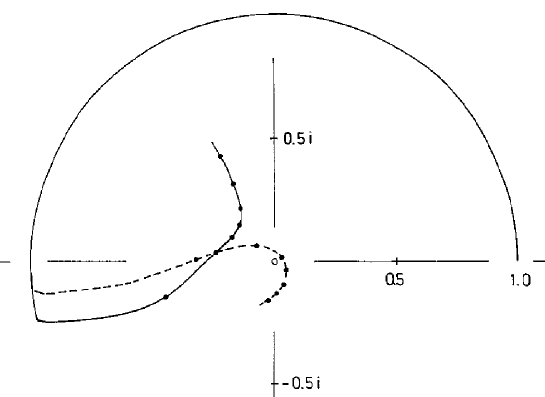
Figure 8: Argand plot of the ${}^{1}S_{0}$ ${t-p}$ $S$-matrix element. The full line represents the $S$-matrix deduced from the $R$-matrix in the complex plane, the broken line the one calculated within the RGM. The dots on the curves denote steps of one MeV in the center-of-mass energy.

The Argand plot of the ${t-p}$ $S$-matrix elements (see fig. 8) hints at the origin of this difference. The diagonal $S$-matrix elements become (very) small in both approaches, due to the underlying $0^{+}$, $T=0$ resonance, discussed above. Since this resonance has almost good isospin $T=0$, the coupling $S$-matrix element between the triton-proton and the ${}^{3}{\rm He}-n$ channel reaches almost the unitary limit of unity. Even at 7.5 MeV the coupling matrix element exceeds the diagonal ones appreciably in both approaches. Since the diagonal $S$-matrix elements are so small, elastic scattering will not allow to determine them more precisely (see discussion below).

From an analysis of the calculated eigenphase shifts together with the background phases for channel radii as given in ref [1], we deduce two additional resonances of almost pure ${d-d}$ structure between 10 and 11 MeV. These resonances do not occur in the recent compilation [1]. The one of ${}^{5}D_{0}$ structure appears already in the model space of only physical channels (see table 6). These high lying resonances of pure ${d-d}$ structure will occur in more partial waves and we will discuss them at the end of this section.

Figure 9: Same as fig. 7, but for the $1^{+}$ phase shifts.

Let us now come to the next partial wave, the $1^{+}$ one. In this partial wave the $R$-matrix analysis [1] finds only one broad resonance about 9 MeV above the ${t-p}$ threshold. Therefore we restricted the RGM calculation to the physical channels only, the ${}^{3}S_{1}$ and ${}^{3}D_{1}$ channels for the [3+1] fragmentations and ${}^{5}D_{1}$ for the deuteron-deuteron channel. In fig. 9 we compare the elastic phase shifts from the $R$-matrix and the RGM for all five channels. All $R$-matrix phases are negative, with the $S$-phase shifts reaching -70 degrees, whereas all $D$-phases do not even reach -15 degrees. The calculated phase shifts are negative too. The $S$-phases agree nicely with the $R$-matrix ones and the $D$-phases are even smaller. From an analysis of the calculated eigenphase shifts together with the background phases for radii as given in ref [1], we again try to deduce resonances. We find in the energy range considered solely a single broad $T=0$ resonance around 11 MeV (see table 6). This is appreciably higher than in the $R$-matrix analysis [1], but the resonance has the same structure.

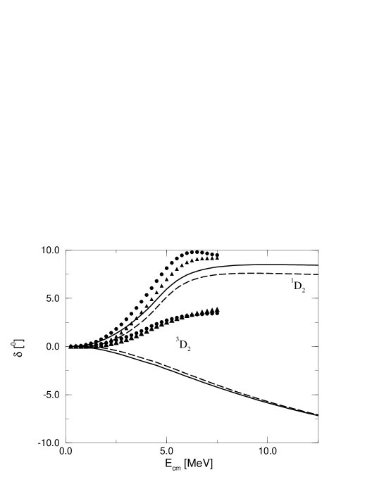
Figure 10: Comparison of $2^{+}$ ${t-p}$ and ${}^{3}{\rm He}-n$ phase shifts.

Since we did not allow for distortion channels, which lead to a stronger coupling of channels in the interaction region, we anticipate that the energy of this resonance would be reduced when distortion channels are included, so that the resonance energies agree more closely.

The $2^{+}$-partial wave contains the most coupled channels. In the $R$-matrix analysis the ${}^{1}D_{2}$ and ${}^{3}D_{2}$ [3+1] fragmentation channels are taken into account together with the ${}^{5}S_{2}$, ${}^{1}D_{2}$, and ${}^{5}D_{2}$ deuteron-deuteron channels. The ${}^{5}G_{2}$ ${d-d}$ channel is neglected. In the RGM calculation, we again restrict ourselves to the physical channels and allow for the same 7 channels. A test calculation [27] including the ${}^{5}G_{2}$ channel, but partially simpler internal functions, yields only minor modifications and is therefore not discussed here. In fig. 10 we compare the $R$-matrix [3+1] phase shifts with those calculated from the RGM. All $R$-matrix phases are positive, the ${}^{1}D_{2}$ reaching almost 10 degrees, with the ${t-p}$ phases a bit larger than the ${}^{3}{\rm He}-n$ ones. The ${}^{3}D_{2}$ phases are quite small, barely reaching 3 degrees. The ${}^{1}D_{2}$ RGM phase shifts agree nicely with the $R$-matrix ones, even so they do not reach quite as high. The ${}^{3}D_{2}$ phases, however, have essentially the opposite sign. It should be noted, however, that a previous $R$-matrix analysis using a somewhat smaller data basis also yielded negative ${}^{3}D_{2}$ phase shifts. The origin of this sign change is not yet known.

Figure 11: Comparison of $2^{+}$ ${d-d}$ phase shifts.

In fig. 11 we present the ${d-d}$ phase shifts. The ${}^{5}S_{2}$ phases fall off strongly and agree perfectly for the two approaches. All $D$-wave phase shifts are small. The $R$-matrix analysis finds positive values at the higher energies, whereas the RGM finds negative values.

In the recent compilation [1] three $2^{+}$ $T=0$ levels are given, all essentially of rather pure ${d-d}$ structure, at 7.6, 8.9, and 10.1 MeV above the ${t-p}$ threshold, having primarily ${}^{5}S_{2}$, ${}^{1}D_{2}$, and ${}^{5}D_{2}$ components. In the RGM calculation, we cannot easily find the complex energy poles of the $S$-matrix, so that the partial widths of the various channels can only be given in case of a Breit-Wigner resonance. We can, however, always diagonalize the $S$-matrix to get the eigenphases and the eigenvectors at all real energies. From these eigenvectors we can determine the isospin value and even its purity of the level under consideration and its structure. In the energy range considered, we find also three $T=0$ resonances, having predominantly ${d-d}$ structure, at 7.3, 10.7, and 11.0 MeV. The structure is the same as found in the $R$-matrix analysis, but the state at 10.7 MeV has also components of ${}^{1}D_{2}$ ${t-p}$ and ${}^{3}{\rm He}-n$ of about 30 percent. Since the width of all these resonances is some MeV [1], the agreement is quite good (see table 6).

For the $3^{+}$ and $4^{+}$ partial waves, the $R$-matrix analysis finds small negative values for all $D$-wave phase shifts for all fragmentations. Till now there is no full-fledged RGM calculation for these partial waves. In order to get an idea what might come out of such a calculation, we used all the matrix elements calculated so far that could be coupled to $3^{+}$ or $4^{+}$. For the [3+1] fragmentations, the resulting internal wave functions are quite good, which can be deduced from the resulting threshold energy, where we loose some hundred keV only. The deuteron-deuteron channels, however, are almost unbound relative to the four-nucleon threshold in the $3^{+}$ case and unbound by more than 3 MeV for the $4^{+}$ channel. This is also reflected in the calculated phase shifts. The ${}^{3}D_{3}$ [3+1] phase shifts are negative and close to their ${}^{3}D_{1}$ and ${}^{3}D_{2}$ counterparts. The ${}^{5}D$ ${d-d}$ phases are tiny and even positive in the $4^{+}$ channel.

Before presenting the negative parity partial waves, let us briefly summarize the results for all $D$-waves. For the ${}^{3}D_{J}$ [3+1] phase shifts, the $R$-matrix yields negative values for $J=1$ and $J=3$, but positive ones for $J=2$. Such a behaviour can be due to a strong tensor force. The RGM calculation yields negative values in all cases with barely any $J$-splitting. Also the splitting of the $R$-matrix ${}^{5}D_{J}$ ${d-d}$ phase shifts follow essentially the pattern of a strong tensor force. The corresponding RGM ones are tiny and show almost no splitting.

Figure 12: Same as fig. 7, but for the $0^{-}$ phase shifts.

Let us now come to the negative-parity partial waves. In the compilation [1] three $0^{-}$ resonances are given. The $R$-matrix analysis takes the ${}^{3}P_{0}$ for the three physical channels into account. In fig. 12 the $R$-matrix phases are compared to the RGM ones. From the steep rise of the ${t-p}$ $R$-matrix data around 1.0 and 4.0 MeV, one can easily conclude the existence of two resonances. The third one, which is of ${d-d}$ structure [1] is not apparent. Except where the [3+1] phases vary rapidly with energy, the ${t-p}$ and ${}^{3}{\rm He}-n$ phases differ essentially by multiples of 180 degrees. Above 4.5 MeV we have added 180 degrees to the ${}^{3}{\rm He}-n$ phase shifts in oder to facilitate the comparison with the RGM results. The RGM calculation takes also the physical channels into account and a few distortion channels of ${d-d}$ structure. As for the $0^{+}$ channels, the [3+1] results look obviously different for the lower energies. At the higher energies they do not quite reach the $R$-matrix phases. The ${d-d}$ phase shifts agree nicely. Similar to the $0^{+}$ partial waves, we anticipate that the resonances with their rather pure isospin are the origin of the differences. As can be seen from the Argand plots in figs. 13 and 14, this is indeed the case. The model space used here corresponds to curve $b$ in figs. 13 and 14. Even though the agreement is not perfect, all the qualitative features agree. Since the $R$-matrix and RGM curves of the $S$-matrix pass on different sides of the origin, one of the phases is increasing and the other decreasing. From the eigenphase shifts we can deduce also three resonances, two of [3+1] structure; a $T=0$ one at 1.6 MeV which has a rather large $T=1$ admixture and a rather pure $T=1$ one at 6.6 MeV, and one of ${d-d}$ structure at 11.1 MeV. These findings agree again nicely with those of ref. [1] (cf. table 6).

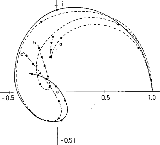
Figure 13: Argand plot of the ${}^{3}P_{0}$ elastic ${t-p}$ $S$-matrix elements extracted from the $R$-matrix (full) and calculated by using the physical channels only (dashed line a), adding 6 ${d-d}$ distortion channels (dashed line b) and adding a total of 46 distortion channels (dashed line c). The origin is marked as a small circle in the middle of the figure.

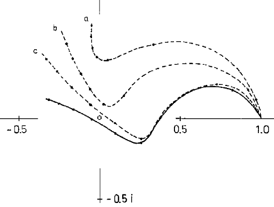
Figure 14: Argand plot of the ${}^{3}P_{0}$ elastic ${}^{3}{\rm He}-n$ $S$-matrix elements extracted from the $R$-matrix (full) and calculated by using the physical channels only (dashed line a), adding 6 ${d-d}$ distortion channels (dashed line b) and adding a total of 46 distortion channels (dashed line c).

In order to demonstrate the effect of changing the model space, we display in figs. 13 and 14 the $S$-matrix elements for elastic triton-proton and ${}^{3}{\rm He}-n$, respectively. For the physical channels only, the RGM results looks quite different for the ${t-p}$ $S$-matrix, even qualitatively. The standard calculation (curve b) displays already all the qualitative features of the $R$-matrix results. The model space of dimension 50 (curves c) reproduces in both cases the $R$-matrix results at low energies perfectly, but crosses the imaginary axis below instead of above the real axis (fig. 13) and vice versa (fig. 14). From these figures it is obvious that small modifications in any of the approaches might change the $S$-matrix a small amount, so that the behaviour near the origin will also qualitatively agree. For the large model space, the resonances are all shifted downward to 1.2, 5.8, and 10.9 MeV, thus agreeing even better with the compilation [1] (see table 6).

The $1^{-}$ phase shifts are displayed in fig. 15. The $R$-matrix data yield positive ${}^{3}P_{1}$ and negative ${}^{1}P_{1}$ [3+1] phases and also negative $d-d$ ones. The extracted level structure is quite rich [1]. The RGM calculation uses all physical channels and a few distortion channels. The results compare favourably with the $R$-matrix ones, even though the ${}^{3}P_{1}$ phases are not quite as large. Allowing for a large number of distortion channels, corresponding to those of the $0^{-}$ partial wave, the positive phases grow up to 45 degrees, and so come into close agreement. From the eigenphase shifts we deduce also four resonances (see table 6), which agree nicely in structure and position with the $R$-matrix ones. It should be noted that the ${}^{3}P_{1}$ [3+1] resonances are strongly isospin mixed.

Figure 15: Same as fig. 7, but for the $1^{-}$ phase shifts.

In the $2^{-}$ partial wave the $R$-matrix allows for $P$- and $F$-waves in all configurations. In fig. 16 the $P$-wave phase shifts are displayed. The [3+1] phases reach about 90 degrees at rather low energies, which indicate the existence of two lying resonances (see ref. [1] and table 6). The ${d-d}$ phases are negative as in the other two negative-parity partial waves. The RGM calculation yields somewhat different results: the positive phase shifts reach only half the $R$-matrix value, whereas the negative ${d-d}$ phases are about a factor two more negative. The extracted resonance positions are still quite reasonable (see table 6).

Figure 16: Same as fig. 7, but for the $2^{-}$ phase shifts.

Since the $R$-matrix analysis allows also for $F$-waves, there are also results for the $3^{-}$ and $4^{-}$ partial waves. The ${}^{1}F_{3}$ phase shifts are negative and reach -4 degrees at the highest energy. The ${}^{3}F_{J}$ phase shifts are all positive or tiny, i.e. in magnitude below 0.2 degrees. The [3+1] ${}^{3}F_{3}$ phase shifts reach up to 7.0 degrees and the ${d-d}$ ${}^{3}F_{4}$ one up to 4.8 degrees, all others are tiny. Resonant structures do not appear. No RGM results exist till now for these partial waves.

For the negative parities the $R$-matrix and RGM phase shifts could be interpreted as due to an effective strong tensor force for the [3+1] fragmentations. Whereas the $R$-matrix results for the ${d-d}$ $F$-waves point more into the direction of a stronger spin-orbit force.

The high lying resonances of ${d-d}$ structure, which occur in almost all partial waves deserve some further discussion. They are not related to any circling of the corresponding $S$-matrix element as in the $0^{+}$ and $0^{-}$ partial waves (see figs. 8, 13, and 14). They are due to the prescription given in ref. [1], where the ${d-d}$ channel has a channel radius of 7.0 fm. This large channel radius leads to rather large background phase shifts, so that around 11 MeV the differences between the eigenphases of the $S$-matrix and the background phase pass through ninety degrees, the criterion we chose for defining the energetic position of a resonance. So it might be that the position of all of these high energy $d-d$ resonances is strongly influenced by the large value of the channel radius. Unfortunately within the RGM we are not aware of any better criterion. This might be the reason, why we find in the RGM calculation also in the $0^{+}$ and $1^{+}$ partial waves resonances around that energy, which have no counterpart in the $R$-matrix analysis (cf. table 6).

6 Comparison with data

In this chapter we compare the various calculations with a wide variety of experimental data. We present figures for all possible elastic scatterings and reactions. Out of the large amount of data, we have selected those energies for which several observables are measured, if possible by different groups. Most of the data presented here are in the data set used to determine the $R$-matrix parameters. We will point out those that are not included in the set. We present results for the $R$-matrix analysis together with RGM calculations. In order to demonstrate the effects of enlarging the model spaces in the calculation we display curves for the largest model space used, denoted by “full”, and for the negative parities for the physical model space only, denoted by “small”. To demonstrate how the calculation using a realistic nucleon-nucleon interaction differs from previous calculations, we display also the results from a previous calculation [4], denoted by “semi-realistic”. Since the $R$-matrix analysis uses most of the data as input values, we consider the $S$-matrix elements determined in this analysis as experimentally determined, despite the fact that the analyis has not yet fully converged. We emphasize the differences of the $S$-matrix elements originating from the $R$-matrix analysis and the full RGM calculation and present the results when we change the value of a specific matrix element from its RGM value to its $R$-matrix value in order to demonstrate that it is just this single matrix element that does not allow to reproduce the data. At the end of this chapter we discuss the various differences and their possible origin. It should be noted that the partial wave analysis of the RGM calculation and the $R$-matrix differ. The $R$-matrix analysis contains additionally the positive-parity contributions for $J^{\pi}=3^{+}$ and $4^{+}$ and all the negative-parity $F$-wave contributions. We will point out in the following in which reactions these differences play a substantial role. The meaning of the lines in all figures is the same as given in fig. 18.

Figure 17: Differential elastic proton-triton cross section calculated at 3.0 MeV $E_{\rm cm}$. The data are for 4.15 MeV protons from ref. [28] (dots) and from ref. [29] (triangles). The full line represents the $R$-matrix analysis, the dashed one the full calculation, the dot-dashed one the small calculation, and the dotted one the semi-realistic calculation. The errors in the data are of the size of the symbols.

Figure 18: Proton analysing power of the reaction ${}^{3}{\rm H}(p,p){{}^{3}{\rm H}}$ calculated for 3.0 MeV $E_{\rm cm}$. The data are for 4.15 MeV protons from ref. [29]. The full line represents the $R$-matrix analysis, the dashed one the full calculation, the dot-dashed one the small calculation, and the dotted one the semi-realistic calculation. The open circles denote the full calculation with the ${}^{3}P_{2}$ matrix element replaced by the corresponding $R$-matrix one.

The various reactions are presented in the order of their thresholds, starting with triton-proton elastic scattering. Here differential cross section and analysing power measurements for the proton and also for the triton exist around 4 MeV proton energy. In fig. 17 we compare the differential cross section data with the various calculations.

Figure 19: Triton analysing power of the reaction ${}^{3}{\rm H}(p,p){{}^{3}{\rm H}}$ calculated for 3.0 MeV $E_{\rm cm}$. The data are for 4.28 MeV protons from ref. [30]. The labeling is the same as in fig. 18.

The $R$-matrix analysis is performed in 250-keV steps of the center-of-mass energy starting from the triton-proton threshold. Since there are no rapid changes with energy of the observables presented, we use the results of the calculations for the nearest energy to that of the data. The error introduced by this procedure is usually well within the experimental error bars. The RGM calculations are also in 250 keV steps of center-of-mass energy, but the calculated thresholds are slightly different (see table 2). From fig. 17 we see that the $R$-matrix analysis reproduces the data quite well. This demonstrates how good the fit to the data is in general. The RGM calculation, on the other hand, reproduces the data reasonably well, taking into account that the calculations contain no adjustable parameters. There are, however, marked deviations from the data. The full calculation using the Bonn potential describes the data much better than the small calculation, but the deviations for forward angles are appreciable.

Figure 20: Differential cross section of the reaction ${\rm{}^{3}H}(p,n)^{3}{\rm He}$ calculated for $E_{cm}=3.0$ MeV. The data are for 4.101 MeV protons from ref. [31]. The labeling is as in fig. 18.

The calculation using the semi-realistic potential describes the forward data very well, but deviates strongly for larger angles. Since we know the $S$-matrix elements from the calculations and the $R$-matrix analysis themselves, we can try to trace the differences to specific $S$-matrix elements. The full calculation differs from the $R$-matrix analysis in the ${}^{3}P_{2}$ matrix element. Note that we represent all $S$-matrix elements in the form $S_{kl}=\eta_{kl}e^{2i\delta_{kl}}$ with phase shifts $\delta_{kl}$ and channel couplings $\eta_{kl}$. In the full calculation, $\eta=0.86$ instead of 0.68 for the $R$-matrix analysis, and the phase shift of 49 degrees misses by 20 degrees the $R$-matrix result; thus the coupling to the ${}^{3}{\rm He}-n$ channels is much weaker. When we use the $R$-matrix ${}^{3}P_{2}$ matrix element instead of the calculated one, the data are very well reproduced. The results lie on top of the $R$-matrix results, therefore we do not display them in fig. 17. The semi-realistic calculation yields a much better ${}^{3}P_{2}$ matrix element. Here the deviations are mainly due to too strong a coupling for the ${}^{3}P_{1}$ matrix element.

Proton analysing power measurements at the same energy as the cross section and nearby triton analysing power data are displayed in figs. 18 and 19, respectively. The $R$-matrix analysis again does an excellent job, whereas the RGM calculation reproduces the data only qualitatively (see figs. 18 and 19). This is again due to the differences in the ${}^{3}P_{2}$ matrix elements (see open circles in figs. 18 and 19), which reproduce the data much better. Note, however, that all calculations yield an analysing power for the proton and the triton that is markedly different in the maximum. This difference is due to the coupling matrix element ${}^{1}P_{1}\rightarrow{{}^{3}P_{1}}$, which is different from zero due to the spin-orbit component of the potentials used. Contrary to the nucleon-nucleon system, such singlet-triplet transitions are not forbidden by the Pauli principle.

The differential cross section for the ${\rm{}^{3}H}(p,n){\rm{}^{3}He}$ reaction at almost the same energy is displayed in fig. 20. Whereas the $R$-matrix reproduces the data quite well, the RGM calculation yields only qualitative agreement with the data, with the increased model space yielding again better agreement. The differences can again be traced to essentially a single matrix element, the already known ${}^{3}P_{2}$ one. For the Bonn potential it reaches only two thirds of the magnitude of the $R$-matrix one, and its relative phase to the ${}^{1}S_{0}$ matrix element is only 60 degrees instead of 80. This just demonstrates the unitarity of the $S$-matrix, i.e. the missing coupling in the elastic triton-proton channel now shows up in the missing strength going from the proton to the neutron channel. All other large matrix elements agree within a few percent in modulus and phase. Changing again in the full calculation the ${}^{3}P_{2}$ matrix element to its $R$-matrix value reproduces the data almost perfectly (cf. fig. 20). Except in the minimum, the modified RGM agrees with the $R$-matrix result. For the semi-realistic potential, the ${}^{3}P_{2}$ matrix element overshoots the $R$-matrix one by 25 percent and the ${}^{3}P_{1}$ one by even 50 percent.

Figure 21: Differential cross section calculated for 8MeV neutrons off ${}^{3}{\rm He}$. The data are for 7.9 MeV neutrons from ref. [33] (dots) and from ref. [32] (triangles) for 8 MeV. The labeling is as in fig. 18.

Figure 22: Neutron analysing power for the scattering of 8 MeV neutrons off ${}^{3}{\rm He}$. Data are from ref. [34] (triangles) and from ref. [35] (dots). The labeling is as in fig. 18.

Elastic neutron scattering cross section and neutron analysing powers around 8 MeV neutron energy are displayed in fig. 21 and fig. 22, respectively. The cross section data are well reproduced not only by the $R$-matrix analysis but also by the full and semi-realistic calculations. Changing in the full calculation again the ${}^{3}P_{2}$ matrix element to its $R$-matrix value brings the results on top of the semi-realistic cross section results.

Figure 23: Differential cross section for the reaction ${}^{2}{\rm H}(d,p){\rm{}^{3}H}$ calculated for $E_{cm}=2.11$ MeV. Data are for 4.0 MeV deuterons from ref. [36] (triangles) and from ref. [37] (dots). The labeling is as in fig. 18.

Figure 24: The analysing power $iT_{11}$ for the reaction ${}^{2}{\rm H}(d,p){\rm{}^{3}H}$ calculated for $E_{cm}=2.11$ MeV. Data are for 4.0 MeV deuterons from ref. [36].The labeling is the same as in fig. 18.

The neutron analysing power, however, is well reproduced by the $R$-matrix, but only qualitatively by the RGM-calculations. The height at the maximum analysing power around 115 degrees is controlled by the phase of the ${}^{3}P_{2}$ matrix element, since the modulus of the matrix elements turns out to be quite similar for all calculations. In the full calculation the phase shift is about 25 degrees below the $R$-matrix analysis (see fig. 16). Increasing the phase of the RGM matrix element by this amount, as was done above for the cross section, reproduces also the analysing power data perfectly. Also the minimum around 90 degrees is well reproduced for this choice. It should be mentioned, however, that the coupling matrix element ${}^{1}P_{1}\rightarrow{{}^{3}P_{1}}$ is only about half the $R$-matrix one, thus leading to a much smaller difference between the neutron and ${}^{3}{\rm He}$ polarisations (compare with the discussion of the charge conjugate scattering ${\rm{}^{3}H}(p,p){\rm{}^{3}H}$ above). There are, however, no ${}^{3}{\rm He}$ polarisation data available, hence one cannot decide about which calculation is correct. All the above elastic neutron scattering data are not included in the $R$-matrix fit, hence, we consider the calculations to be predictions.

Let us now come to the deuteron induced reactions. In fig. 23 the ${\rm{}^{2}H}(d,p){\rm{}^{3}H}$ differential cross section is displayed. The data are well reproduced by all calculations. Here for the first time the small calculation reproduces the data even better than the full calculation. The semi-realistic calculation overshoots the data a bit. At the forward (and backward) angles, the $F$-waves, which are missing in the RGM calculations, contribute about 50 percent to the cross section in the $R$-matrix analysis and indicate that even G-waves may be necessary.

In figs. 24, 25, 26, and 27 the deuteron analysing powers are displayed. Whereas the $R$-matrix analysis describes the data nicely, the RGM calculations fail completely. In the $R$-matrix analysis the dominant matrix elements are the ${}^{3}P_{1}$, ${}^{1}D_{2}$, and the ${}^{5}S_{2}\rightarrow{{}^{3}D_{2}}$ matrix elements, but also quite a number of others must not be neglected, like the ${}^{1}S_{0}$ and the ${}^{5}S_{2}\rightarrow{{}^{1}D_{2}}$. The coupling matrix element ${}^{5}S_{2}\rightarrow{{}^{3}D_{2}}$ determines essentially the form of the angular distribution of all polarisation observables. The $R$-matrix analysis finds this matrix element to half of the leading ${}^{3}P_{1}$ one and the relative phase shift to be +60 degrees. The full RGM calculation yields, however, only a quarter of the leading matrix element and the relative phase shift of -33 degrees, i.e. the opposite sign. The ${}^{1}S_{0}$ and ${}^{3}P_{2}$ overshoot the $R$-matrix result by a factor 2 to 3. The other RGM calculations give similar results. Changing the RGM coupling matrix element ${}^{5}S_{2}\rightarrow{{}^{3}D_{2}}$ to the $R$-matrix value yields reasonable agreement for the vector polarisation data (cf. fig. 24) and improves the angular form of the tensor analysing powers (cf. figs. 25, 26, and 27). For the forward angles the calculation comes now much closer to the data, but the shape of the angular distribution does not match. The reason for this discrepancy can be found in the interference terms of the large and the smaller matrix elements. The $R$-matrix analysis indicates that for a detailed description of these data, the $F$-wave contributions are necessary. The modified cross section turns out to be slightly too large.

For the ${\rm{}^{2}H}(d,n){\rm{}^{3}He}$ reaction, data exist for the same energy as for the charge conjugate ${\rm{}^{2}H}(d,p){\rm{}^{3}H}$ reaction. In fig. 28 we compare the differential cross section data with the various calculations. The $R$-matrix analysis again does a perfect job. Also the full RGM calculation reproduces the data nicely, whereas the semi-realistic one overshoots the data appreciably. The dominant matrix elements are again ${}^{3}P_{1}$, ${}^{1}D_{2}$, and ${}^{5}S_{2}\rightarrow{{}^{3}D_{2}}$ in the $R$-matrix analysis, but also the ${}^{1}S_{0}$, ${}^{3}P_{2}$, and ${}^{5}S_{2}\rightarrow{{}^{1}D_{2}}$ being of equal magnitude, must not be neglected. The full RGM calculation yields the two dominant matrix elements similarly, but the coupling matrix elements ${}^{5}S_{2}\rightarrow{{}^{3}D_{2}}$ and also ${}^{5}S_{2}\rightarrow{{}^{1}D_{2}}$ are only half of the $R$-matrix value. On the other hand, the ${}^{1}S_{0}$ and ${}^{3}P_{2}$ ones are doubled, as is the case of the charge conjugate reaction.

Figure 25: Same as fig. 24, but for the analysing power $T_{20}$.

Figure 26: Same as fig. 24, but for the analysing power $T_{21}$.

Figure 27: Same as fig. 24, but for the analysing power $T_{22}$.

Figure 28: Differential cross section for the reaction ${}^{2}{\rm H}(d,n){\rm{}^{3}He}$ calculated for $E_{cm}=2.11$ MeV. Data are for 4.0 MeV deuterons from ref. [37]. The labeling is as in fig. 18.

Figure 29: The deuteron vector analysing power for the reaction ${}^{2}{\rm H}(d,n){\rm{}^{3}He}$ calculated for $E_{cm}=2.11$ MeV. Data are for 4.0 MeV deuterons from ref. [38].The labeling is the same as in fig. 17.

Figure 30: Same as fig. 29, but for the analysing power $A_{zz}$.

The Ohio-State group [38] has measured all deuteron polarisation observables also for 4.0 MeV deuterons. In figs. 29 and 30, we present only the vector analysing power and $A_{zz}$ data, because the overall behaviour is quite similar to the charge conjugate reaction.

As in the charge conjugate reaction ${\rm{}^{2}H}(d,p){\rm{}^{3}H}$, only the $R$-matrix analysis reproduces the data, whereas all RGM calculations fail completely. To find such a good agreement with data, the ${}^{3}F_{3}$ and ${}^{3}F_{4}$ matrix elements in the $R$-matrix are vital. Again the ${}^{5}S_{2}\rightarrow{{}^{3}D_{2}}$ matrix element is dominating the angular form of all analysing powers. Using in the full RGM calculation the corresponding ${}^{5}S_{2}\rightarrow{{}^{3}D_{2}}$ matrix element from the $R$-matrix does not reproduce the data much better. Here it is also neccessary to modify the corresponding ${}^{5}S_{2}\rightarrow{{}^{1}D_{2}}$ matrix element. Then the cross section is not changed at all, the vector analysing power is reproduced reasonably well, but for the description of the tensor polarisations, not too much is gained (cf. figs. 29 and 30). Note that in the RGM no $F$-waves are included.

Figure 31: Differential cross section for elastic deuteron-deuteron scattering calculated for $E_{cm}=3.11$ MeV. Data are for 6.0 MeV deuterons from ref. [39]. The labeling is as in fig. 17.

Let us now discuss the last two-fragment process, elastic deuteron-deuteron scattering. Because of the identical bosons in the entrance and exit channel, the vector polarisation and $T_{21}$ are antisymmetric and all other observables are symmetric about 90 degrees. Since the data are usually converted into the forward hemisphere we display this part only in the following figures. In fig. 31 we present rather old data [39] for the differential cross section together with the calculations. The $R$-matrix analysis reproduces the data very well. The two realistic RGM calculations lying on top of each other also reproduce the data reasonably well, the semi-realistic calculation, however, overshoots the data appreciably.

Figure 32: Vector analysing power $iT_{11}$ for elastic deuteron-deuteron scattering calculated for $E_{cm}=3.11$ MeV. Data are for 6.0 MeV deuterons from ref. [40]. The labeling is as in fig. 17.

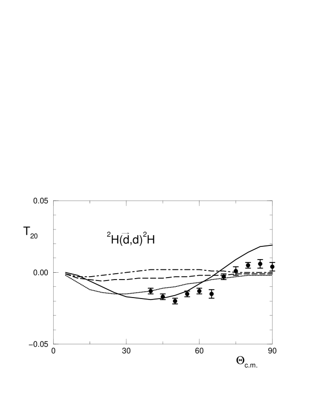
Figure 33: Same as fig. 32 but for the tensor analysing power $T_{20}$.

The analysing powers have been measured by the Zürich group [40]. In figs. 32, 33, 34, and 35 we compare the data with various calculations. All polarisations are quite small, of the order of one or two percent. Note the large scale on the figures. Except for the tensor polarisation $T_{22}$, where all calculations fail, the $R$-matrix analysis reproduces the data well. Considering the small values, also the full calculation reproduces the data reasonably well. Since the polarisations are so small, it is useless to search for the matrix element(s), which dominate the structure of the polarisations. It has to be mentioned, however, that the inclusion of these tiny polarisations into the $R$-matrix analysis changed the sign in the ${}^{3}D_{2}$ triton-proton and neutron-${}^{3}{\rm He}$ elastic matrix elements (see the above discussion following fig. 10).

Figure 34: Same as fig. 32, but for the tensor analysing power $T_{21}$.

Figure 35: Same as fig. 32, but for the tensor analysing power $T_{22}$.

Considering all the figures displaying a comparison of data and calculations together, it is obvious that the parameter-free calculations reproduce the differential cross sections rather well, whereas the polarisations are sometimes grossly missed. The differences in the description of the data between the $R$-matrix analysis and the RGM-calculations are concentrated in a few $S$-matrix elements. In order to reproduce the data the calculated ${}^{3}P_{2}$ matrix elements for all channels and the ${}^{5}S_{2}\rightarrow{{}^{3}D_{2}}$ and the ${}^{5}S_{2}\rightarrow{{}^{1}D_{2}}$ matrix element in the deuteron-deuteron fusion reaction have to be changed. In the ${}^{3}P_{2}$ one, the coupling to the $F$-waves cannot be totally neglected. So in both cases the tensor force is crucial for the determination of these matrix elements, because the coupling is to channels with a different orbital angular momentum. As discussed in the previous chapter, the $R$-matrix analysis indicates a rather strong tensor force. It might therefore be that the Bonn potential is the origin for the discrepancies of the RGM calculation with data. That the tensor component in the Bonn potential is rather weak has been pointed out many times, e.g. [41].

7 Conclusion and Outlook

We performed microscopic multi-channel calculations employing an $r$-space version of the realistic Bonn potential in the framework of the resonating group model. This is a parameter-free calculation in a rather large model space, chosen by physical arguments and restricted by computational limitations. For the ground state it is essentially a variational calculation, with the functional form of the wave function dictated by the following scattering calculation.

For the ground state energy we got almost the same results as were obtained using variational wave functions [3] for the same potential. The extracted point Coulomb form factor agrees nicely with that of a variational calculation [24] using another realistic nucleon-nucleon potential. Restricting the model space to those parts appropriate for bound state wave functions, we could determine properties of the first excited state and also the point Coulomb form factor. From the properties we concluded that this resonance is not a breathing mode and gave arguments why the energy of this resonance in shell model calculations differs from that determined from scattering experiments. Also the form factor deviates strongly from that of the ground state.

From the scattering calculations we extracted phase shifts and demonstrated that the parameter-free calculation yields not only qualitatively, but in most cases even quantitatively, the same answers as the $R$-matrix analysis using only data. In some cases we showed that the apparent differences of the two methods are caused by only minor variations of the $S$-matrix elements near the origin. The other deviations appear in channels that can be strongly influenced by the tensor-force terms in the nucleon-nucleon interaction. Since it is well known that the potential we used has a rather weak tensor component [41], we blame the potential for those differences. Extracting resonance positions in an analogous way to the recent compilation [1] yielded close agreement in the sequence, quantum numbers, and structure of the resonances. Near the upper limit of the energy interval considered, the difference between eigenphases of mainly deuteron-deuteron structure and background phase shifts passed through ninety degrees, the accepted criterion for the position of a resonance. In these cases, however, the interpretation as a resonance seems to be doubtful.

Finally we compared the various calculations with data. All differential cross sections were well reproduced, especially if we used the largest model space. The polarisation observables, however, revealed the shortcomings mentioned above. Only after modifying in most cases a single $S$-matrix element, the agreement between calculation and data became satisfactory. For the $d-d$ fusion reaction, however, $F$-wave contributions that could not be taken into account and the interference effects with smaller matrix elements prevented a reasonable agreement.

Taking all this information together, the parameter-free microscopic calculations using a realistic nucleon-nucleon force are very promising in explaining and even predicting data. The shortcomings discussed above indicate the direction of further studies. Increasing the model space brings calculations and data in closer agreement (cf. figs. 17 to 35), but the essential deviations between $R$-matrix analysis and RGM calculations are untouched. Since we suspect the nucleon-nucleon potential is responsible for these deviations, it is necessary to use another potential with a stronger tensor component. Since the RGM requires the potential to be given in $r$-space, we consider the Argonne AV14 [42] the proper choice, especially because there exist many calculations of ground state properties for light nuclei with this potential. Furthermore, results for this two-body potential supplemented by various three-body potentials are also available. Work in this direction is under way.

Acknowledgements: Both authors wish to acknowledge the hospitality of various institutions, where part of the work was done: Los Alamos National Laboratory, where all this work started quite some time ago, while one of us (H. M. H.) was on sabbatical, the ECT*/Trento, where most of the manuscript was written, and Triangle Universities Nuclear Laboratory, where final preparation of the manuscript took place. This work would not have been possible without the support in part by funds from the U. S. Department of Energy Division of Nuclear Physics (G. M. H.) and from the Deutsche Forschungsgemeinschaft, the BMFT and the BMBF (H. M. H.).

Appendix A Appendix 1: Wave functions of the fragments

The general structure of the wave functions is given in eqs. (1) and (2) (for further details see [8, 13]). For the deuteron we have used the most simple wave function. Since the spin part is trivial, we give just the orbital part.

$$\psi_{D}=\sum_{n=1}^{3}c_{n}e^{-\beta_{n}/2\;({\bf r}_{1}-{\bf r}_{2})^{2}}\;{\cal Y}_{0}({\bf r}_{1}-{\bf r}_{2})\;+\sum_{n=4}^{5}c_{n}e^{-\beta_{n}/2\;({\bf r}_{1}-{\bf r}_{2})^{2}}\;{\cal Y}_{2}({\bf r}_{1}-{\bf r}_{2})$$ (14)

Here $\cal Y$ denote solid spherical harmonics [27] . The width parameters $\beta_{n}$ and the coefficients $c_{n}$ for the deuteron and the singlet deuteron $d\raisebox{3.01385pt}{-}$ are given in table 7.

Table 7: Deuteron and singlet deuteron parameters

n	1	2	3	4	5
$\beta_{n}$	5.8359	0.5201	0.0684	1.625	0.4339
$c_{d}$	6.239420	-6.659597	-2.370518	-6.685710	-0.7940629
$c_{\bar{d}}$	-4.491821	3.059319	3.018020	0	0

The spatial part of the three-nucleon wave functions is of the form

$$\psi_{3N}=\sum_{l_{1},l_{2},L,n,m}\;c_{n,m}^{\left[l_{1},l_{2}\right]L}\;e^{-\beta_{n}s_{1}^{2}}\;e^{-\beta_{m}s_{2}^{2}}\;{\cal{Y}}_{l_{1}}({\bf s}_{1})\;{\cal{Y}}_{l_{2}}({\bf s}_{2})\;\phi^{S}$$ (15)

where $\phi^{S}$ denotes the appropriate spin functions of each term in the sum. The Jacobian coordinates are given by

$${\bf s}_{1}=\frac{1}{\sqrt{2}}({\bf r}_{1}-{\bf r}_{2})\;\;\mbox{ and }\;\;{\bf s}_{2}=\frac{1}{\sqrt{6}}({\bf r}_{1}+{\bf r}_{2})\;-\sqrt{\frac{2}{3}}\;{\bf r}_{3}$$ (16)

The width parameters $\beta_{n}$ and $\beta_{m}$ for triton and ${}^{3}{\rm He}$ are given in table 8.

Table 8: Triton and ${}^{3}{\rm He}$ width parameters

k	1	2	3	4	5	6
$\beta_{n}^{{}^{3}{\rm H}}$	4.972	0.8659	0.1531	8.665	1.8056	0.5414
$\beta_{m}^{{}^{3}{\rm H}}$	3.293	0.3972	0.07513	1.626	0.4745	0.09417
$\beta_{n}^{{}^{3}{\rm He}}$	4.8887	0.8286	0.1493	8.354	1.939	0.61723
$\beta_{m}^{{}^{3}{\rm He}}$	3.616	0.3822	0.06763	1.546	0.4668	0.09258

The first three parameters belong to the structures containing no $D$-waves and the last three width parameters belong to those containing at least one $D$-wave.

Appendix B Appendix 2: Minimal ${}^{4}{\rm\bf He}$ Wave Function

Since the full bound state wave function of the ${}^{4}{\rm He}$ ground state contains 227 different configurations, it is too complicated to be given in detail. To give an impression about the dominant structures of the ground state wave function, we will describe in some detail the minimal wave function of table 5. It consists of 20 configurations, where 11 originate from the physical channels, which have been resolved into its constituents, and 9 are former distortion channels. All of them have orbital angular momentum zero on the relative coordinate between the fragments, but as can be seen in table 5, all spin values are present. For the relative motion we choose 5 width parameters, used also for all distortion channels irrespective of the fragmentation, with the values: 2.433, 0.8214, 0.2987, 0.1185, 0.05001 in units of ${\rm fm}^{-2}$. For the internal width parameters of the fragments the parameters given in tables 7 and 8 are used.

The dominant $S=0$ contribution contains 11 configurations: In the triton-proton fragmentation, the three containing no internal angular momentum from the physical channel and also the combination with the proton-neutron pair inside the triton coupled to spin=1, but with the coefficients for the various internal width parameters taken for the third exited state. The ${}^{3}{\rm He}-n$ fragmentation contains the analogous three contributions from the physical channel. From the distortion channels we also find the vector with the internal proton-neutron pair of $S=1$, but here the second and third excited states appear with large expansion coefficients, indicating that together with some other state they are numerically almost linearly dependent. For the deuteron-deuteron fragmentation none of the physical components contribute. The $S$-wave part of the deuteron, together with the $S$-wave part of the first and second excited states of the deuteron, form the remaining two channels. The overlap of the components originating from the physical channels with the total wave function is in excess of 90 percent. The overlap of the configurations containing excited fragment wave functions is only about 84-85 percent, whereas the one containing the first excited state of the deuteron has less than 10 percent.

The next important $S=2$ contribution contains 8 configurations: For the triton-proton fragmentation only the two configurations with one internal angular momentum being two, the other zero, originating from the physical channel, contribute. For the ${}^{3}{\rm He}-n$ fragmentation, the configuration with $P$-waves on both internal coordinates and that with a $D$-wave between the internal neutron-proton pair contribute from the physical channel. From the distortion channels the two configurations with one internal $D$-wave, with the coefficients from the first excited state contribute. For the deuteron-deuteron fragmentation, the $S$-wave part of the deuteron and the $D$-wave of the deuteron and the first excited state of the deuteron form the two contributing channels. The overlap of the various components with the total wave function varies between 3 percent for the $d-d$ distortion channel and 27 percent for the ${}^{3}{\rm He}$ $D$-wave physical channel.

The $S=1$ component is formed from the $D$-wave part of the deuteron and the $D$-wave of the first excited state, coupled to spin equal one.

References

- [1] D.R. Tilley, H.R. Weller and G.M. Hale, Nucl. Phys. A541 (1992) 1
- [2] G.M. Hale, D.C. Dodder and K. Witte (unpublished)
- [3] J. Carlson, Phys. Rev. C38 (1988) 1879
- [4] H.M. Hofmann, W. Zahn and H. Stöwe, Nucl. Phys. A357 (1981) 139
- [5] M. Baumgartner, H.P. Gubler, M. Heller, G R. Plattner, W. Roser and I. Sick, Nucl. Phys. A368 (1981) 189
- [6] S. Fiarman and W.E. Meyerhof, Nucl. Phys. A206 (1973) 1
- [7] R. Machleidt, K. Holinde and Ch. Elster, Phys. Rep. C149 (1987) 1
- [8] H.M. Hofmann, in: Models and Methods in Few-Body Physics, eds. L. S. Ferreira et al., Lecture Notes in Physics 273, Springer, Heidelberg 1987
- [9] K. Wildermuth and Y.C. Tang, A Unified Theory of the Nucleus, Vieweg, Braunschweig 1977
- [10] Y. C. Tang, in: Topics in Nuclear Physics, Lecture Notes in Physics 145, Springer, Heidelberg 1981
- [11] H. Kellermann, H.M. Hofmann and Ch. Elster, Few-Body Sys. 7 (1989) 31
- [12] H. Eikemeier and H.H. Hackenbroich, Nucl. Phys. A169 (1971) 407
- [13] H.M. Hofmann, in Finite Systems and Multiparticle Dynamics, vol. 3, D. A. Micha and F. S. Levin eds., Plenum to be published
- [14] W. Kohn, Phys. Rev. 74 (1948) 1763
- [15] G.M. Hale et al. (1989) (unpublished)
- [16] G.M. Hale et al. (1983) (unpublished)
- [17] W. Heitler, The Quantum Theory of Radiation, Oxford University Press 1954
- [18] E.P. Wigner and L. Eisenbud, Phys. Rev. 72 (1947) 29; A.M. Lane and R.G. Thomas, Rev. Mod. Phys. 30 (1958) 257
- [19] G.M. Hale, R.E. Brown and N. Jarmie, Phys. Rev. Lett. 59 (1987) 763
- [20] P.E. Koehler et al., Phys. Rev. C37 (1988) 917
- [21] R.J. Eden and J.R. Taylor, Phys. Rev. B133 (1964) 1575
- [22] A.R. Edmonds, Angular Momentum in Quantum Mechanics, Princeton University Press 1960
- [23] R. Ceulener, P. Vandepeutte and C. Semay, Phys. Rev. C38 (1988) 2335
- [24] R. Schiavilla, V.R. Pandharipande and D.O. Riska, Phys. Rev. C41 (1990) 309
- [25] R.G. Arnold et al., Phys. Rev. Lett. 40 (1978) 1429
- [26] R.F. Frosch et al., Phys. Rev. 160 (1968) 874
- [27] E.L. Tomusiak, W. Leidemann and H.M. Hofmann, Phys. Rev. C52 (1995) 1963
- [28] R. Detomo et al., unpublished data from Ohio State University; private communication from T. Donoghue (1978)
- [29] R. Kankowsky, J.C. Fritz, K. Kilian, A. Neufert and D. Fick, Nucl. Phys. A263 (1976) 29
- [30] R.F. Haglund, Jr., R.E. Brown, N. Jarmie, G.G. Ohlsen, P.A. Schmelzbach and D. Fick, Phys. Lett. 79B (1978) 35
- [31] J.E. Perry, Jr. et al. (unpublished), reported by J.D. Seagrave in Proceedings of the Conference on Nuclear Forces and the Few Nucleon Problem, London (1959)
- [32] B. Haesner, Dissertation, Kernforschungszentrum Karlsruhe (August 1982); private communication from H. Klages (1995)
- [33] M. Drosg, D.K. McDaniels, J.C. Hopkins, J.D. Seagrave, R.H. Sherman and E.C. Kerr, Phys. Rev. C9 (1974) 179
- [34] L. Drigo, G. Tornielli and G. Zannoni, Ann. Phys. 7 (1982) 408
- [35] P.W. Lisowski, C.T. Rhea and R.L. Walter, Nucl. Phys. A259 (1976) 61
- [36] W. Grüebler, V. König, P.A. Schmelzbach, R. Risler, R.E. White and P. Marmier, Nucl. Phys. A193 (1972) 129
- [37] R.L. Schulte, M. Cosack, A.W. Obst and J.L Weil, Nucl. Phys. A192 (1972) 609
- [38] L.J. Dries, H.W. Clark, R. Detomo, Jr. and T.R. Donoghue, Phys. Lett. 80B (1979) 176
- [39] J.E. Brolley, Jr., T.M. Putnam, L. Rosen and L. Stewart, Phys. Rev. 117 (1960) 1307
- [40] W. Grüebler, V. König, R. Risler, P.A. Schmelzbach, R.E. White and P. Marmier, Nucl. Phys. A193 (1972) 149
- [41] R. Machleidt, Adv. Nucl. Phys. 19 (1991) 230
- [42] R.B. Wiringa, R.A. Smith and T.L. Ainsworth, Phys. Rev. C 29 (1984) 1207