Full $pf$ shell study of $A=47$ and $A=49$ nuclei

Abstract

Complete diagonalizations in the $pf$ major shell, lead to very good agreement with the experimental data (level schemes, transitions rates, and static moments) for the $A=47$ and $A=49$ isotopes of Ca, Sc, Ti, V, Cr, and Mn. Gamow-Teller and M1 strength functions are calculated. The necessary monopole modifications to the realistic interactions are shown to be critically tested by the spectroscopic factors for one particle transfer from ⁴⁸Ca, reproduced in detail by the calculations. The collective behaviour of ⁴⁷Ti, and of the mirror pairs ⁴⁷V–⁴⁷Cr and ⁴⁹Cr–⁴⁹Mn is found to follow at low spins the particle plus rotor model. It is then analysed in terms of the approximate quasi-SU(3) symmetry, for which some new results are given.

]

I INTRODUCTION

In a recent paper [1] hereafter referred as I, the A=48 nuclei were studied through exact diagonalizations in the full $pf$ shell, using a realistic interaction whose monopole centroids had been minimally modified to cure the bad saturation properties characteristic of all forces that describe adequately the NN phase shifts. Close agreement with experiment was obtained for the observables (level schemes, static moments and electromagnetic transitions) near the ground states, and at higher energies as shown by Gamow Teller strength functions calculated for A=48 and other nuclei in the region [2, 3].

One of the most interesting findings in [1] was the backbending behaviour of ⁴⁸Cr, simultaneously established experimentally [4], and reminiscent of energy patterns hitherto found only in much heavier rotational nuclei. In ref. [5] the question was treated in some detail, establishing the equivalence of shell model and mean field treatments, and a similar study is now avilable for ⁵⁰Cr [6]. Recent experiments indicate that the agreement with the calculated yrast energies in ⁴⁸Cr has become almost perfect, and further data on the collective properties in the A=46-50 region are forthcoming [7].

It appears that an exhaustive study of the A=47 and A=49 nuclei along the lines of I, and using the same interaction, is a natural next step. This paper is devoted to it, and it is organized so as to address three basic issues:

  Detailed spectroscopy

A much decried aspect of Nuclear Physics, often referred to as “zoology”, but nevertheless an essential test of the quality of the calculations. This test is notoriously more difficult to pass in odd nuclei.

  The interaction

It is of interest to illustrate why it is sufficient to study closed shell nuclei, and the single-particle and single-hole excitations based on them, to obtain the monopole modifications that transform the realistic interactions into successful ones.

  Collective properties

The behaviour of yrast lines in rotor-like nuclei did not seem amenable to exact shell model diagonalizations. Since the A=46-50 region offers a counter example, it is well worth going into it in some detail.

Accordingly, we shall proceed as follows:

Section II will be devoted to detailed spectroscopy by comparing calculations with the impressive body of data in Burrows’s compilation [8, 9, 10]. The agreement turns out to be particularly satisfactory when the experimental results are unambiguous, suggesting that the calculations become useful guides in the cases of difficult assignments.

Section III deals with Gamow Teller and M1 strength functions. Though there are no measures of these quantities some of them may be of special interest. In particular ⁴⁷Ti is predicted to exhibit a strong “scissors”-like excitation.

In section IV we analyze the spectroscopic factors for one particle transfer from ⁴⁸Ca to ⁴⁹Ca and ⁴⁹Sc, and explain their direct bearing on the minimal monopole modifications that cure the problems of the Kuo Brown interaction (KB) [11], transforming it into the successful variant that we use (KB3) [12, 13, 14, 15].

Rotational properties of the two mirror pairs obtained by adding or removing a particle from ⁴⁸Cr will be studied in section V. It will be seen that several low lying bands are almost perfectly described—up to some critical spin—by strong particle (or hole)-rotor couplings. The microscopic mechanisms at the origin of the collective behaviour can be understood in terms of quasi-SU(3) [16], and some time will be devoted to explaining how this approximate symmetry works.

Throughout the paper, $f$ stands for $f_{7/2}$ (except of course when we speak of the $pf$ shell) and $r$, generically, for any or all of the other subshells ($p_{1/2}\;p_{3/2}\;f_{5/2}$). Spaces of the type

$$f^{n-n_{0}}r^{n_{0}}+f^{n-n_{0}-1}r^{n_{0}+1}+\cdots+f^{n-n_{0}-t}r^{n_{0}+t}$$ (1)

represent possible truncations: $n_{0}$ is different from zero if more than 8 neutrons (or protons) are present and when $t=n-n_{0}$ we have the full space $(pf)^{n}$ for $A=40+n$.

We use: harmonic oscillator wave functions with $b=1.01A^{1/6}$ fm; bare electromagnetic factors in $M1$ transitions; effective charges of 1.5 $e$ for protons and 0.5 $e$ for neutrons in the electric quadrupole transitions and moments.

Other definitions and conventions are introduced at the beginning of the sections in which they are first needed.

II Level schemes and electromagnetic properties

The diagonalizations are done with the code antoine [17], a fast implementation of the Lanczos algorithm in the $m$-scheme. Some details may be found in ref. [18]. The interaction KB3 is the same as in I, and it will be revisited in section IV. The $m$-scheme and maximal $JT$ dimensions of the nuclei analyzed are given in table I.

A Energy Levels in A=47

⁴⁷Ca. Calculated and experimental levels are compared in fig. 1. The ambiguities in the experimental spin assignments make it difficult to pass judgement on the agreement, except that it seems fair.

⁴⁷Sc (fig. 2). In this nucleus the experimental situation is cleaner and the agreement striking. Notice the very nice correspondence for the high spin states.

⁴⁷Ti (fig. 3). The stable member of the $A=47$ isobaric multiplet is the best known experimentally. We have plotted all the calculated and measured levels of negative parity up to 4 MeV. From there up, only the yrast or the ones with high spin, relevant to the discussion below are included. There is an excellent correspondence between theory and experiment; the ground state doublet, the triplet around 1.5 MeV and the two bunches of levels at 2.5 and 3.7 MeV. In the high spin regime, Cameron and collaborators [19] have identified two states at 6.366 and 8.005 MeV. They propose spins $\frac{21}{2}^{-}$ and $\frac{27}{2}^{-}$ while our calculation favours $\frac{19}{2}^{-}$ and $\frac{25}{2}^{-}$ in line with the assignments made in Burrows’ compilation [8]. The yrast sequence will be discussed in detail in section V.

⁴⁷V and ⁴⁷Cr (fig. 4). The almost degererate ground state triplet of these nuclei is one of the hard nuts to crack in $pf$-shell spectroscopy. In the MBZ [21] model, i.e. a single $1f_{\frac{7}{2}}$ shell and the ⁴²Sc two-body matrix elements as effective interaction, the state $\frac{3}{2}^{-}$ appears at an excitation energy of 1.2 MeV above the $\frac{5}{2}^{-}$-$\frac{7}{2}^{-}$ ground state doublet. The perturbative quasiconfiguration calculation of [15](using the KB3 interaction) brought the $\frac{3}{2}^{-}$ state down to 0.5 MeV, but it takes the exact $pf$ shell diagonalization to give the correct ordering $\frac{3}{2}^{-}$, $\frac{5}{2}^{-}$, $\frac{7}{2}^{-}$. A $\frac{3}{2}^{-}$ ground state is consistent with ⁴⁷V being a K=$\frac{3}{2}$ rotor. The theoretical level scheme fits perfectly to the experiment except for a couple of doublets that come out inverted.

B Electromagnetic Moments and Transitions in A=47

In table II we collect our predictions for the magnetic dipole and electric quadrupole moments to compare with the availabe experimental values. The agreement is very good, except for $Q$ in ⁴⁷Ca. For ⁴⁷V and ⁴⁷Cr no experimental results are known.

For ⁴⁷Ca, there is an experimental upper bound to the probability of the transition $3/2^{-}$ $\rightarrow$ $7/2^{-}$; $B(E2)<2.8$ $e^{2}$ fm⁴, that is compatible with the predicted value (0.68 $e^{2}$ fm⁴). Tables III, IV and V display the E2 and M1 transition probabilities in ⁴⁷Sc, ⁴⁷Ti and ⁴⁷V. The data are of poor quality, but in general compatible with our results, though there is a tendency for quadrupole transitions between low-lying levels to be stronger than our predictions indicate. This effect can be probably attributed to mixing with the intruder excitations of the ⁴⁰Ca core.

C Energy Levels in A=49

⁴⁹Ca and ⁴⁹Sc. These nuclei will be discussed in section IV.

⁴⁹Ti is the stable member of the $A=49$ isobaric multiplet. It is interesting to compare fig. 5 for this nucleus with fig. 2 for ⁴⁷Sc, its cross-conjugate in the $f^{n}$ model, which would predict identical spectra. There are similarities indeed, but there are also significant differences. The quality of the agreement with experiment is high in both cases. Fig. 5 deserves a special comment: it was drawn using the information of the 1986 compilation of ref. [9]. In the 1995 version the level immediately above 1.6 MeV that was given as $(5/2,7/2,9/2)^{-}$ becomes a doublet ${5/2}^{-}$-${9/2}^{-}$ leading to a one to one corresponce with the calculations below 2 MeV, except for the new ${5/2^{-}}$ level—a possible intruder. However, the next two levels that were taken to be either ${5/2}^{-}$ or ${7/2}^{-}$ in both cases, are now given a tentative ${5/2}^{-}$ assignment, while the calculations would obviously prefer ${7/2}^{-}$ …

⁴⁹V is our showpiece: the quality of the agreement in figure 6 is simply amazing.

⁴⁹Cr and ⁴⁹Mn. The left panel of fig. 7 indicates that up to the second 19/2^- state there is a one to one correspondence between the experimental levels and the theoretical ones with an excellent agreement in energies. The data are consistent with a $K=5/2$ rotor as we shall explain in section V. The yrast states above 7 MeV in ⁴⁹Cr, taken from a recent experiment [20], appear to be 2 MeV above the calculated ones, a discrepancy well beyond the typical deviations of our results. Furthermore, in the $f^{n}$ space ⁴⁷V and ⁴⁹Cr are cross conjugate and have the same spectra: It would be a real surprise to find a 25/2^-- 27/2^- doublet 2 MeV higher in Chromium than in Vanadium. There seem to be two ways out of the conundrum.

• Assume the states are not yrast. The calculations have been pushed to include several states for each $J$, and some tentative correspondencess—based on energetics and decay properties— are indicated in the figure by dot-dash lines. The identifications are hazardous, and we prefer the alternative explanation.

• Assume the states are yrast. Then some gamma(s) may have been misplaced in the level scheme. The right panel of fig. 7 shows what would be the situation if the $J=23/2^{-}$ level was taken to decay to the first (lowest) $J=19/2^{-}$ instead of the second (as assumed in [20]). Cross conjugation is now respected, and the agreement with the calculation becomes excellent. Therefore we shall adopt this interpretation of the spectrum in the discussion in section V.

D Electromagnetic Moments and Transitions in A=49

The experimental information about magnetic moments is collected in Table VI. In all cases the predictions agree with the data, including the very recently measured moment of the 19/2^- isomeric state in ⁴⁹Cr. The only known $Q$ nicely agrees with the calculated one.

In tables VII, VIII and IX we find the experimental information on $E2$ and $M1$ transitions for the $A=49$ isotopes of Ti, V, and Cr. ( The data available for the other members of the multiplet are too imprecise to compare with the calculation.) The agreement is in general excellent, and in particular for the $B(E2)$ values in ⁴⁹V and ⁴⁹Cr and the $B(M1)$ transition probabilities in ⁴⁹Cr.

From this review of detailed properties it is possible to draw a general conclusion: the calculations are very successful in describing the data, the only systematic exceptions coming from the Ca isotopes: The agreement in fig. 1 is probably the less satisfactory of all we have shown, and in table II the magnetic moment of ⁴⁷Ca is the only one that deviates significantly from the measured ones. In I we had already had problems with the positioning and B(E2) value for the $2^{+}$ state of ⁴⁸Ca, and in section IV we shall also encounter some discrepancies of monopole origin in ⁴⁹Ca. When corrected, the agreement with experiment will no doubt improve, but it seems almost certain that a full understanding of the Ca isotopes demands a closer look at the influence of intruders.

III M1 and GT strength functions

In this section we shall calculate strength functions following Whitehead’s prescription [22]. The procedure amounts to define a “sum rule state” by acting with the transition operator we are interested in ( M1 or GT here, single particle creation operator in next section) and then use it as starting state for Lanczos iterations. At the $n$-th iteration $n$ peaks are obtained that contain full information on the $2n-1$ moments of the strength distribution. The sum rule is the norm of the starting state. For more detailed explanations and illustrations the reader is referred to [23, 24, 25].

For the M1 strength we write

$$B(M1)=\left(\sqrt{B}_{l}\pm\sqrt{B}_{s}\right)^{2},$$ (2)

where the $l$ and $s$ subscripts correspond to orbital and spin contributions respectively.

The Gamow-Teller (GT) strength is defined through

$$B(GT)=\left(\frac{g_{A}}{g_{V}}\right)^{2}_{\text{eff}}\langle\mathchoice{{\hbox{\boldmath$\displaystyle\sigma\tau$}}}{{\hbox{\boldmath$\textstyle\sigma\tau$}}}{{\hbox{\boldmath$\scriptstyle\sigma\tau$}}}{{\hbox{\boldmath$\scriptscriptstyle\sigma\tau$}}}\rangle^{2},\hskip 14.22636pt\langle\mathchoice{{\hbox{\boldmath$\displaystyle\sigma\tau$}}}{{\hbox{\boldmath$\textstyle\sigma\tau$}}}{{\hbox{\boldmath$\scriptstyle\sigma\tau$}}}{{\hbox{\boldmath$\scriptscriptstyle\sigma\tau$}}}\rangle=\frac{\langle f||\sum_{k}\mathchoice{{\hbox{\boldmath$\displaystyle\sigma$}}}{{\hbox{\boldmath$\textstyle\sigma$}}}{{\hbox{\boldmath$\scriptstyle\sigma$}}}{{\hbox{\boldmath$\scriptscriptstyle\sigma$}}}^{k}\mathchoice{{\hbox{\boldmath$\displaystyle t$}}}{{\hbox{\boldmath$\textstyle t$}}}{{\hbox{\boldmath$\scriptstyle t$}}}{{\hbox{\boldmath$\scriptscriptstyle t$}}}^{k}_{\pm}||i\rangle}{\sqrt{2J_{i}+1}},$$ (3)

where the matrix element is reduced with respect to the spin operator only (Racah convention [26]), $\pm$ refers to $\beta^{\pm}$ decay, $\mathchoice{{\hbox{\boldmath$\displaystyle t$}}}{{\hbox{\boldmath$\textstyle t$}}}{{\hbox{\boldmath$\scriptstyle t$}}}{{\hbox{\boldmath$\scriptscriptstyle t$}}}_{\pm}=(\mathchoice{{\hbox{\boldmath$\displaystyle\tau$}}}{{\hbox{\boldmath$\textstyle\tau$}}}{{\hbox{\boldmath$\scriptstyle\tau$}}}{{\hbox{\boldmath$\scriptscriptstyle\tau$}}}_{x}\pm\text{i}\mathchoice{{\hbox{\boldmath$\displaystyle\tau$}}}{{\hbox{\boldmath$\textstyle\tau$}}}{{\hbox{\boldmath$\scriptstyle\tau$}}}{{\hbox{\boldmath$\scriptscriptstyle\tau$}}}_{y})/2$, with $\mathchoice{{\hbox{\boldmath$\displaystyle t$}}}{{\hbox{\boldmath$\textstyle t$}}}{{\hbox{\boldmath$\scriptstyle t$}}}{{\hbox{\boldmath$\scriptscriptstyle t$}}}_{+}p=n$ and $(g_{A}/g_{V})_{\text{eff}}$ is the effective axial to vector ratio for GT decays,

$$\left(\frac{g_{A}}{g_{V}}\right)_{\text{eff}}=0.77\left(\frac{g_{A}}{g_{V}}\right)_{\text{bare}},$$ (4)

with $(g_{A}/g_{V})_{\text{bare}}=1.2599(25)$ [27];

for Fermi decays we have

$$B(F)=\langle\mathchoice{{\hbox{\boldmath$\displaystyle\tau$}}}{{\hbox{\boldmath$\textstyle\tau$}}}{{\hbox{\boldmath$\scriptstyle\tau$}}}{{\hbox{\boldmath$\scriptscriptstyle\tau$}}}\rangle^{2},\hskip 28.45274pt\langle\tau\rangle=\frac{\langle f||\sum_{k}\mathchoice{{\hbox{\boldmath$\displaystyle t$}}}{{\hbox{\boldmath$\textstyle t$}}}{{\hbox{\boldmath$\scriptstyle t$}}}{{\hbox{\boldmath$\scriptscriptstyle t$}}}^{k}_{\pm}||i\rangle}{\sqrt{2J_{i}+1}};$$ (5)

Half-lives, $T_{1/2}$, are found through

$$(f_{A}+f^{\epsilon})\,T_{1/2}=\frac{6146\pm 6}{(f_{V}/f_{A})B(F)+B(GT)}.$$ (6)

We follow ref. [28] in the calculation of the $f_{A}$ and $f_{V}$ integrals and ref. [29] for $f^{\epsilon}$. The experimental energies are used.

A Scissors mode in ⁴⁷Ti

The existence of magnetic dipole orbital excitations in deformed nuclei has been a topic of interest since the discovery of the “scissors” mode in heavy nuclei [32]. It was suggested by Zamick and Liu [33] that scissors-like excitations coud also exist in lighter nuclei. In a study of ⁴⁶Ti and ⁴⁸Ti [18] it was found that the low lying 1⁺ states of these nuclei has indeed orbital character. In odd nuclei the strength can split in up to three $J$ values. Since experiments can be done only for stable targets, we have repeated the calculations for ⁴⁷Ti and ⁴⁹Ti. For the latter, nothing very interesting seems to happen, since quadrupole collectivity—an essential ingredient in scissor-like behaviour—is practically absent. For the former, quadrupole coherence is fairly strong, as we shall see in section V A. Therefore we restrict ourselves to showing in fig. 8 the orbital, spin and total $M1$ strength functions of ⁴⁷Ti. Notice the very different structure of the orbital and spin strengths. The former is dominated by the peaks at around 2 MeV while the latter is basically a resonace centered at about 9 MeV with a much smaller peak at low energy. In the total strength the two regions show up. The large spikes in the orbital strength are the natural candidates to represent the scissors mode. The angular momentum, excitation energy and strength of these states are:

$J$	E (MeV)	Orbital	Spin	Total
7/2-	2.34	0.162	0.229	0.776
3/2-	2.37	0.092	0.093	0.370

The values of the ratio $B_{l}/B_{s}$, 1.0 and 0.7 (using bare gyromagnetic factors), strongly support the scissors interpretation of these magnetic dipole excitations.

B Half-lives and Gamow-Teller strength functions

We denote the total strength in the $\beta^{+}$ or $(n,p)$ channel by $S_{+}$ and the strength in the $\beta^{-}$ or $(p,n)$ channel by $S_{-}$. We express them in units of the Gamow-Teller sum rule so that they satisfy $S_{-}-S_{+}=3(N-Z)$. From past experience we know that even severely truncated calculations may give a sensible view of the overall strength distributions, but miss the sum rule values by a sizeable factor [1, 3]. To have a fuller picture we have compared exact results with those of the most severe truncation compatible with the $3(N-Z)$ sum rule, $t=0$ in the father and $t=1$ in the daughters (notation defined in eq. (1)) . The results are compiled in table X incorporating the numbers we had for $A=48$. There is, in all cases, a strong reduction of the $S_{+}$ strength. The reduction factor is fairly constant for each isotopic chain and all the values are close to 2. This is probably a good estimate of the reduction of strength to be expected in the general case due to $0\hbar\omega$ correlations.

The half-lives of the $A=47$ isobars are known up to ⁴⁷Cr. In table XI we compare our calculations (using the effective value of $g_{A}$) with the experimental values. Agreement is perfect for Ca, Sc and Cr and fair for V. For the proton richer nuclei the half-lives are not known and we list our predictions alone. For the $Z>N$ nuclei we also show the percentage of intensity that goes to the analog state by a Fermi transition. Where it is experimentally known (⁴⁷Cr) the agreement with the predicted value is very good. In table XII we proceed in the same way with the $A=49$ multiplet. All the calculated half-lives have been measured. The agreement is close to perfect for all the short ones. Very long half-lives usually mean that the decay window is very small and the fraction of strength allotted to it is very critical, which probably explains the discrepancies in the Ca and V cases.

Figure 9 shows the strength function for the processes ⁴⁷Sc$(\beta^{-}){}^{47}$Ti and ⁴⁷Fe$(\beta^{+}){}^{47}$Mn. The spikes that come out of the Lanczos strength function have been smoothed by gaussians of 500 keV full width half maximum (FWHM) if they correspond to converged or quasi-converged states and 1.3 MeV otherwise. The Fe to Mn decay— not studied experimentally yet—has a very large $Q_{\beta}$ window ($Q_{\text{EC}}=15.64$ MeV) that covers an important fraction of the full strength. On the contrary, only the small bump at around 0 MeV in the strength function contributes to the ⁴⁷Sc decay (here we are lucky and the half-life comes out on the experimental spot).

Next, we show the strength functions corresponding to the—not yet performed—reactions ⁴⁷Ti$(p,n){}^{47}$V and ⁴⁷Ti$(n,p){}^{47}$Sc (figure 10). We have followed different procedures to present the distributions of the $(p,n)$ and $(n,p)$ processes. For the former, the individual peaks are broadened by Gaussians whose width is taken to be equal to the typical instrumental one for these reactions. For the latter, the spikes have been replaced by gaussians with FWHM=1 MeV, and then we have summed up the strength in 1 MeV bins. We show the original spikes as reference. The upper part of the figure contains the strength function obtained in a $t=1$ calculation. It is similar in structure to the full calculation (lower left part) though the resonance is shifted down by some 2.5 MeV. For the reactions ⁴⁹Ti$(p,n){}^{49}$V and ⁴⁹Ti$(n,p){}^{49}$Sc, figure 11 shows that the $t$=1 calculation gives a fair idea of the exact distribution, but the Gamow-Teller resonance is again shifted down by some 2-3 MeV.

Comparing the exact $(p,n)$ profiles in figures 10 and 11 we find that the GT resonance is definitely broader in ⁴⁷Ti than in ⁴⁹Ti. The effect does not show in the truncated calculations, which suggests that the extra broadening should be associated to deformation—absent in ⁴⁹Ti—but significant in ⁴⁷Ti as we shall see in section V.

IV Spectroscopic Factors in ⁴⁹Sc and ⁴⁹Ca. The KB3 interaction.

The monopole modifications that cure the defficiencies of the KB matrix elements and transform them into the excellent KB3 interaction can be characterized by a single prescription:

make sure to have correct gaps and correct single particle properties in ⁴⁸Ca and ⁵⁶Ni.

Our purpose in this section is to analyse in detail this prescription.

A Elementary monopole results

The reason to single out closed shells and single-particle and single-hole states built on them ($cs\pm 1$ for short) is that we know to a good approximation their eigenstates, whose energies are given in terms of the few parameters that define the “monopole” Hamiltonian. Writing $H=H_{m}+H_{M}$, as a sum of monopole($m$) and multipole($M$) parts, and calling $n_{r}$ and $T_{r}$ the number and isospin operators for orbit $r$ of degeneracy $D_{r}=2(2j_{r}+1)$, $V_{rstu}^{JT}$ the two-body matrix elements and $\varepsilon_{r}$ the single particle energies , we have  [34]:

$$H_{m}=\sum_{r}\varepsilon_{r}n_{r}+$$ (8)

$$\sum_{r\leq s}(1+\delta_{rs})^{-1}[a_{rs}\,n_{r}(n_{s}-\delta_{rs})+b_{rs}(T_{r}\cdot T_{s}-\frac{3}{4}n\delta_{rs})],$$ (9)

$$a_{rs}=\frac{1}{4}(3V^{1}_{rs}+V^{0}_{rs}),\quad b_{rs}=V^{1}_{rs}-V^{0}_{rs},$$ (10)

where the “centroids” are:

$$V_{rs}^{T}=\frac{\sum_{J}V_{rsrs}^{JT}(2J+1)}{\sum_{J}(2J+1)}.$$ (11)

The sums run over Pauli allowed values of $J$. The important property of $H_{m}$ is that it reproduces the average energies of the configurations to which a given state belongs. For the $cs\pm 1$ set, there is only one state per configuration, and therefore its energy is exactly given by $H_{m}$.

Calling $f\equiv f_{7/2}$, $p\equiv p_{3/2}$, $r\equiv p_{3/2},p_{1/2},f_{5/2}$, and $r^{\prime}\equiv p_{1/2},f_{5/2}$, from eqs. (8) and (10) we find the following estimates for binding energies ($B_{e}$), single particle gaps ($\Delta$) and excitation energies ($\epsilon$):

$$B_{e}(^{48}\text{Ca})=8\varepsilon_{f}+28V^{1}_{ff}.$$ (12)

$$B_{e}(^{56}\text{Ni})=16\varepsilon_{f}+120a_{ff}-6b_{ff}.$$ (13)

$$\text{$\Delta$}(^{48}\text{Ca}) = -2B_{e}(^{48}\text{Ca})+B_{e}(^{49}\text{Ca})+B_{e}(^{47}\text{Ca})$$ (14)

$$= \varepsilon_{p}-\varepsilon_{f}+8V_{fp}^{1}-7V_{ff}^{1}.$$ (15)

$$\text{$\Delta$}(^{56}\text{Ni}) = -2B_{e}(^{56}\text{Ni})+B_{e}(^{57}\text{Ni})+B_{e}(^{55}\text{Ni})$$ (16)

$$= \varepsilon_{p}-\varepsilon_{f}+16a_{fp}-15a_{ff}+\frac{3}{4}b_{ff}.$$ (17)

$$\epsilon_{r^{\prime}}(^{49}\text{Ca})=\varepsilon_{r^{\prime}}-\varepsilon_{p}+8(V^{1}_{fr^{\prime}}-V^{1}_{fp}).$$ (18)

$$\epsilon_{r}(^{49}\text{Sc})=\varepsilon_{r}-\varepsilon_{f}+8(a_{fr}-a_{ff})-\frac{5}{2}(b_{fr}-b_{ff}).$$ (19)

$$\epsilon_{r^{\prime}}(^{57}\text{Ni})=\varepsilon_{r^{\prime}}-\varepsilon_{p}+16(a_{fr^{\prime}}-a_{fp}).$$ (20)

NOTE In work on masses—to avoid minus signs—it is customary to take $B_{e}>0$ for bound systems. Here we keep $B_{e}<0$, but reverse the definition of $\Delta$ so as to conform with the usual one ($\Delta>0$ means the closed shell is more bound).

The expressions above are useful guides, but the $a_{rs}$ and $b_{rs}$ parameters must be chosen so that the exact diagonalizations reproduce the binding and excitation energies. At the time the monopole modifications to KB were proposed the task involved some guessing, that can now be eliminated, and it is instructive to reexamine critically the KB3 interaction, which was defined in three steps [12, 13, 14, 15]:

  KB’

The $V_{fr}^{T}$ centroids.

$$V_{fr}^{T}(\text{KB'})=V_{fr}^{T}(\text{KB})-(-)^{T}\,300\text{ keV},$$ (21)

  KB1

The $V_{ff}^{T}$ centroids ($V_{fr}^{T}$ centroids from KB’)

$$\begin{array}[]{l}V_{ff}^{0}(\text{KB1})=V_{ff}^{0}(\text{KB})-350\text{ keV},\\[5.69054pt] V_{ff}^{1}(\text{KB1})=V_{ff}^{1}(\text{KB})-110\text{ keV}.\end{array}$$ (22)

  KB3

KB1 plus minor non-monopole changes.

$$\begin{array}[]{l}W_{ffff}^{J0}(\text{KB3})=W_{ffff}^{J0}(\text{KB1})-300\text{ keV for $J=1,3$};\\[5.69054pt] W_{ffff}^{21}(\text{KB3})=W_{ffff}^{21}(\text{KB1})-200\text{ keV}.\end{array}$$ (23)

while the other matrix elements are modified so as to keep the centroids (22). These very mild changes were made to improve the spectroscopy of some nuclei at the beginning of the $pf$ shell. Their limited influence is discussed in I, and we shall not bother with them in this paper.

To give an idea of the influence of the monopole changes: Eqs. (15) and (17) yield

$\Delta$(⁴⁸Ca)=2.06 MeV, and $\Delta$(⁵⁶Ni)=3.42 MeV for KB,

$\Delta$(⁴⁸Ca)=4.46 MeV, and $\Delta$(⁵⁶Ni)=5.86 MeV for KB’,

$\Delta$(⁴⁸Ca)=5.22 MeV, and $\Delta$(⁵⁶Ni)=8.57 MeV for KB3,

to be compared with experimental values

$\Delta$(⁴⁸Ca)=4.81 MeV, and $\Delta$(⁵⁶Ni)=6.30 MeV (exp).

If we turn to the exact calculations, we find that $\Delta$(⁴⁸Ca), for KB increases by some 600 keV, while for KB’ and KB3 it hardly moves! For KB3 it actually goes down to 5.17 MeV. For ⁵⁶Ni, the situation is more difficult to assess because full diagonalizations are not possible yet. Still, going to the $t=4$ level reveals that for KB, instead of a closed shell we have a nice rotational band dominated by 4p-4h configurations. At the same level of truncation the KB’ ground state remains normal but we are still far from convergence, and at $t=6$ it produces in turn a rotational ground state. KB3 yields $\Delta$(⁵⁶Ni)=7.90 MeV, and extrapolation to the exact result indicates that the closed shell will persist with the gap remaining above the experimental one by about 1 MeV [3].

B Spectra and spectroscopic factors

Let us now examine the spectrum of ⁴⁹Ca. In fig. 12 we show the results for KB, KB’ and KB3. The unmodified interaction predicts 10 levels below 3.2 MeV, where two are observed. The remarkable thing is that with the change in $V^{1}_{fr}$—involving a single parameter—KB’ produces a phenomenal improvement. The remaining discrepancies are eliminated by one extra modification in $V^{1}_{ff}$: The quality of agreement with experiment achieved by KB3 is excellent for the levels below 4.1 MeV, with two possible exceptions:

The calculations predict two ${7/2}^{-}$ levels at 3.04 and 4.09 MeV with very small spectroscopic factors for $(d,p)$ transfer, but still sufficient to be observed. Both are strongly dominated by the $f^{7}p^{2}$ configuration, and very unlikely to move up by more than a few hundred keV. Now: there are possible experimental counterparts at 3.35 and 4.1 MeV, assigned as ${9/2}^{+}$ and ${7/2}^{+}$ respectively. We think there is room for revising these assignments, especially for the first of the two states.

For ⁵⁶Ni we have not gone beyond the calculations in [3], which indicate that the single particle spectrum is quite adequately described by KB3. As made clear by eqs. (19) and (20), ⁴⁹Sc should provide the same information about centroids as ⁵⁷Ni. Fig. 13 does not seem very encouraging in this respect: Although there is a nice correspondence between theory and experiment for the first bunch of levels around 4 MeV, it is impossible to read from the spectra alone any clear message about single particle excitations, and hence about monopole behaviour. The reason is that the states we are interested in,

$$|r\rangle=a^{{\dagger}}_{r}|^{48}\text{Ca gs}\rangle,$$ (24)

are heavily fragmented. The amplitude of vector $|r\rangle$ in each of the fragments is essentially the spectroscopic factor, defined as

$$S(j,t_{z})=\frac{\langle J_{f}T_{f}T_{zf}||a^{{\dagger}}_{jt_{z}}||J_{i}T_{i}T_{zi}\rangle^{2}}{2J_{f}+1},$$ (25)

where the matrix element is reduced in angular momentum only; $j$ and $t_{z}$ refer to the spin and third isospin component of the stripped nucleon. To calculate $S(j,t_{z})$ we proceed as in section III: use $|r\rangle$ as starting vector for a sequence of Lanczos iterations.

The excitation energies of the starting vectors, $e_{r}=\langle r|H|r\rangle-\langle f|H|f\rangle$, (in MeV)

$$e_{p_{3/2}}=4.54\quad e_{p_{1/2}}=5.99\quad e_{f_{5/2}}=5.76,$$ (26)

are almost identical to the values obtained through eq. (19):

$$\epsilon_{p_{3/2}}=4.58\quad\epsilon_{p_{1/2}}=5.99\quad\epsilon_{f_{5/2}}=5.66,$$ (27)

a result readily explained by the weakness of the ground state correlations in ⁴⁸Ca. By the same token the sum rules for $(2j+1)S(j,t_{z})$ are very close to their theoretical maximum, $(2j+1)$. It may be worth mentioning here that the the sum rule is actually quenched by a factor of about 0.7 because of the deep correlations that take us out of the model space. The problem is discussed in detail in ref. [2], and shall be ignored here.

The spectroscopic factors for $f_{7/2}$ in fig. 14, show little fragmentation. For $p_{3/2}$, fig. 15 seems to indicate a discrepancy between theory—that produces substantial fragmentation—and experiment, that falls quite short of the sum rule, by detecting basically only two peaks. Note that the higher, at around 11.5 MeV, corresponds to the IAS of the ground state of ⁴⁹Ca. The discrepancy is explained when we consider fig. 16 for the $p_{1/2}$ strength: now the too numerous experimental fragments abundantly exceed the sum rule. What seems to be happening is that the method chosen to analyse the data does not distinguish among the $L=1$ peaks those with $J=1/2$ from those with $J=3/2$, unduly favouring the former.

Note that the lowest calculated state is a bit too high in fig. 16. (The higher states are again isobaric analogues.)

The situation becomes truly satisfactory for the $f_{5/2}$ strength in fig. 17. The four lowest theoretical peaks may demand a slight downward shift but they have nearly perfect counterparts in experiment, where a fifth state also shows—a probable intruder. Higher up the agreement remains quite good, especially if we remember that, at 60 iterations, the spikes beyond 7 MeV do not represent converged eigenstates but doorways, subject to further fragmentation. Note that it is the second of the two IAS levels slightly above 15 MeV that carries most of the strength.

It is clear that in the $J=1/2$ and 3/2 spectra, the lowest state in each is sufficiently dominant to be identified as the single particle state, while for $J=5/2$, this object has been replaced by a bunch of levels at around 5 MeV. In all cases the calculations are too high by some 300 to 500 keV, indicating unperturbed positions in eq. (19) too high by about this amount: A residual monopole defect that should be corrected. However, it is worth noting that the main strength (i.e., the single particle states, and the 5/2 multiplet) has already been pushed down by about 1 MeV. This is a genuine dynamical effect—abundantly studied in the literature under the name of “particle-vibration coupling ”—which amounts to stress that when a particle is added to a “core”, it couples not only to its ground state, but also to its excitations.

What we have shown in this section is a fully worked out realistic example of how the displacement and fragmentation of the original “doorway” states, $|r\rangle$, takes place. In the language of Landau’s theory one would speak of bare particles becoming dressed quasi-particles, and it is one of the merits of exact shell model calculations to be able to illustrate in detail this subtle dressing process.

C A critical assessment of KB3

Our basic tenet is that once $H_{m}$ provides the correct unperturbed energies, the residual $H_{M}$ takes good care of the mixing. It is particularly well illustrated by the study of the spectroscopic factors, where both the unperturbed positioning ($H_{m}$) and the fragmentation mechanism ($H_{M}$) are crucial. Other properties —in particular collective ones—are, usually, not as sensitive to monopole behaviour, and if they are, it may be more difficult to have a clearcut picture of the relative influence of $H_{m}$ and $H_{M}$. What we are aiming at, is that the place to look for monopole problems and cures is in the $cs\pm 1$ states: From what we have seen in this section, good gaps and single particle properties around ⁴⁸Ca are sufficient to ensure that the interaction is good for the nuclei at the beginning of the $pf$ shell.

The outstanding problems seem relatively minor: the gap in ⁵⁶Ni should be reduced by about 1 MeV, and the $\epsilon_{r}$ values in eq. (27) should be reduced by some 300 to 500 keV. The gap in ⁴⁸Ca needs also a reduction of some 300 keV and some gentle tampering with $\epsilon_{r}$ values in ⁴⁹Ca may be warranted. The necessary changes amount basically to making $a_{fr}-a_{ff}$ more attactive by 50 keV or so.

There is a serious problem though, with the KB3 interaction: the $V^{T}_{rr^{\prime}}$ centroids were left untouched, because for the nuclei we had been interested in, their influence was small and difficult to detect. In a sense this was a blessing since it simplified the task of doing the monopole corrections. However, to move beyond ⁵⁶Ni it is necessary to do the corrections, because—as was pointed out by Brown and Ormand [35]—the single hole properties of KB3 around ⁷⁹Zr are atrocious, and the reader is warned not to rely on this interaction above A$\approx$60 . We shall not go into the problem here, and simply refer to a forthcoming characterization of $H_{m}$,—in terms of very few parameters—valid for the whole periodic table [36].

D Binding energies

In I it was noted that KB3 overbinds all A=48 nuclei by about 780 keV and it was proposed to cure the problem by a monopole correction of 28.85$n(n-1)/2$ keV. Calculating Coulomb energies, as in I, through the following expressions $(n=\pi+\nu,\pi$ = protons, $\nu$ = neutrons) [12]

$$\begin{array}[]{cc}\lx@intercol\hfil\displaystyle{H_{\text{Coul}}=\frac{\pi(\pi-1)}{2}V_{\pi\pi}+\pi\nu V_{\pi\nu}+7.279\pi\text{ MeV,}}\hfil\lx@intercol\\[8.53581pt] \displaystyle{V_{\pi\pi}=0.300\,(50)\text{ MeV,}}&\displaystyle{V_{\pi\nu}=-0.065\,(15)}\text{ MeV,}\end{array}$$ (28)

we obtain binding energies relative to the ⁴⁰Ca core as listed in table XIII for A=47 and in table XIV for A=49. (Here we use the convention that binding energies are positive). The agreement with the measured values is quite good, the larger discrepancies coreesponding to the estimates based on systematics [37].

V Collective properties.

The collective model [38] provides a framework for the study of the shape oscillations to which nuclei are subjected under one form or another. In general, the coupling between different modes precludes the sort of general predictions that are possible in the extreme cases, and we shall start by examining ⁴⁷Ti, which is definitely collective, but neither a rotor nor a vibrator. Then we move on to ⁴⁹Cr-⁴⁹Mn and ⁴⁷V-⁴⁷Cr, for which the strong coupling limit should apply. Following I, a good rotor will be characterized by a $J(J+1)$ energy sequence and by a constant intrinsic quadrupole moment $Q_{0}$ for all members of the band. In addition to being a constant, we expect $Q_{0}$ to be the same when extracted from the spectroscopic quadrupole moment through

$$Q_{0}=\frac{(J+1)\,(2J+3)}{3K^{2}-J(J+1)}\,Q_{spec}(J),\hskip 14.22636pt\text{for {\hbox{K\neq 1}}}$$ (29)

or from the BE2 transitions through the rotational model prescription (for $K\neq\frac{1}{2},1$)

$$B(E2,J\;\rightarrow\;J-2)=\frac{5}{16\pi}\,e^{2}|\langle JK20|J-2,K\rangle|^{2}\,Q_{0}^{2}.$$ (30)

For even-even nuclei this is about as far as we can go in deciding whether we are faced with a good rotor or not. When a particle is added or removed, the collective model description of its coupling to the rotor leads to some very precise predictions that make the comparison with microscopic calculations more stringent. In section V B we are going to see that the low spin states in the ⁴⁹Cr-⁴⁹Mn and ⁴⁷V-⁴⁷Cr mirror pairs follow these predictions quite well. Then, a change of regime takes place and the calculations remain in agreement with experiment but the strong coupling limit of the collective model ceases to be valid.

By what should we replace it?

From the studies of ^48,50Cr [5, 6], we know how the change of regime—associated with backbend— takes place, and there is a framework—quasi-SU(3) [16]—that describes yrast behaviour before and after backbend. We shall devote some time to it in section V C.

A Incipient collectivity in ⁴⁷Ti.

Quadrupole collectivity is not confined to “good rotors”. There are other species that include “vibrators”, “$\gamma$-soft nuclei” and the like. ⁴⁸Ti was found in I to be one of those nuclei that are definitely collective, but definitely not rotors. Its neighbour ⁴⁷Ti belongs to the same category: In figure 18 we have plotted the experimental excitation energies against angular momentum (open circles). A $J(J+1)$ law (open triangles) was fitted to these points. The rms deviation is 313 keV and the static moment of inertia ${\cal J}^{(1)}=11$ MeV^-1. The largest distortions take place at spins $\frac{7}{2}^{-}$ and $\frac{9}{2}^{-}$. Clearly, there is a rotational flavour, but it is not fully convincing. If now we turn to the quadrupole moments, extracting $Q_{0}$ for the yrast states from eqs. (29) and (30) we find the results shown in table XV. The $Q_{0}$ values coming from the spectroscopic moments are quite erratic, while those obtained from the $B(E2)$’s are closer to constancy at around $Q_{0}=60$ e fm², similar to the number found in ⁴⁸Ti. Therefore, though we do not have a good rotor, the structure of the yrast band of ⁴⁷Ti suggests the existence of an incipient prolate intrinsic state.

Are we in the presence of a “new form of collectivity”?

In attempting to give an answer, we may remember that Bohr’s collective Hamiltonian was precisely designed to cope with such intermediate coupling situations (see appendix 6B of [38]). Unfortunately, they demand the specification of potential energy surfaces and inertial parameters that can be (meaningfully) determined only in terms of “some” underlying microscopic Hamiltonian.

Now: we have a reliable Hamiltonian that has proven capable of describing whatever form of collectivity present in a given nucleus. It also happens that the collectivity seems to be predominantly quadrupole. Therefore, before (or perhaps, instead of) answering the question above we should do well to examine the following one(s):

What is the collective part of the Hamiltonian? How does it work?

Section V C will be devoted to this problem.

B Particle-rotor coupling in ⁴⁹Cr-⁴⁹Mn and ⁴⁷V-⁴⁷Cr

Since ⁴⁸Cr seems to be a reasonably good rotor at low spins, we expect the two mirror pairs obtained by adding and removing a particle from it to be reasonably well described by the strong coupling limit particle plus rotor model. In their simplest form, the predictions would be the following:

  Energies

The bands should have the same moment of the inertia as the underlying rotor. Coriolis decoupling is expected to be appreciable only in $K=1/2$ bands (not our case)

  Deformations

The quadrupole moments should be the same as those of the underlying rotor.

  Magnetic moments

The contribution of the extra particle (or hole) is now crucial, and can largely exceed that of the rotor. The precise prediction will be discussed in section V B 2.

At first we restrict ourselves to presenting evidence on these three items. Conclusions will be drawn at the end of the section.

1 Energetics and quadrupole properties

The yrast levels in figures 4 and 7 have been fitted to a $J(J+1)$ law, with the results shown in fig. 19. For ⁴⁷V the agreement is quite good for all spins , using a static moment of inertia, ${\cal J}^{(1)}=12$ MeV^-1. For ⁴⁹Cr only the states with $J\leq 17/2$ where included in the fit, yielding, ${\cal J}^{(1)}=8$ MeV^-1. The energies of the states with $J\geq 19/2$ seem to behave as a strongly decoupled rotational band of high $K$, but the quadrupole moments and transitions do not support this interpretation.

The results of applying eqs. (29) and (30) to the $K=3/2$ and $K=5/2$ bands in the ⁴⁷V-⁴⁷Cr and ⁴⁹Cr-⁴⁹Mn pairs respectively are given in tables XVI and XVII . For the lowest states the values are close to the ones obtained for ⁴⁸Cr in ref. [1] ($Q_{0}(2^{+})=103\ e$ fm²), which is indeed what we expect in the particle plus rotor model, but the situation is somewhat different for the two pairs:

• ⁴⁷V-⁴⁷Cr. For $Q_{0}$ extracted from $Q_{s}$ there is a curious staggering effect for the lower spins that does not show for the $BE2$-extracted numbers. The anomaly at $J=17/2$ is due to the presence of an almost degenerate state of this spin (refer to fig 4). Beyond this spin, $Q_{0}$ decreases but not drastically. In view of the good $J(J+1)$ behaviour for all spins, one may be tempted to conclude that there is no significant change of regime along the yrast line. The study of the gyromagnetic factors will tell us soon that this is not so.

• ⁴⁹Cr-⁴⁹Mn. Here the situation is simpler, and similar to that of ⁴⁸Cr: A plot of $J\,vs\,E_{\gamma}$ would show a backbend at $J=17/2$. Beyond this spin the $f_{7/2}^{n}$ configuration becomes strongly dominant and $Q_{0}$ behaves erratically, and there are indications—to be confirmed by the gyromagnetic factors—that the change of regime starts at $J=13/2$, i.e., before the backbend.

2 Gyromagnetic factors

A very interesting test of the validity of the collective model comes from the magnetic moments, for which the predicted contributions of the particle (or hole) and the rotor are of similar magnitude.

For the gyromagnetic factors of a $K$-band we have:

$$g(J)=g_{R}+(g_{K}-g_{R})\frac{K^{2}}{J(J+1)},\hskip 14.22636pt\text{for {\hbox{K\neq\frac{1}{2}}}};$$ (31)

where $g_{R}$ is the rotor gyromagnetic factor and $g_{K}$ is defined by

$$g_{K}K=\langle\Phi_{K}|g_{l}\mathchoice{{\hbox{\boldmath$\displaystyle l$}}}{{\hbox{\boldmath$\textstyle l$}}}{{\hbox{\boldmath$\scriptstyle l$}}}{{\hbox{\boldmath$\scriptscriptstyle l$}}}_{3}+g_{s}\mathchoice{{\hbox{\boldmath$\displaystyle s$}}}{{\hbox{\boldmath$\textstyle s$}}}{{\hbox{\boldmath$\scriptstyle s$}}}{{\hbox{\boldmath$\scriptscriptstyle s$}}}_{3}|\Phi_{K}\rangle.$$ (32)

$|\Phi_{K}\rangle$ is the intrinsic wave function of the particle, corresponding to a Nilsson orbit of quantum numbers $[Nn_{z}m_{l}]K$. Using the asymptotic wavefunctions we find

$$g_{K}=g_{s}+(g_{l}-g_{s})\frac{m_{l}}{K}$$ (33)

To compare the shell model results with eq. (31) we have to extract $g_{R}$ and $g_{K}$ from our wave functions. As a first step, let us decompose the gyromagnetic factors as a sum of isoscalar ($g_{0}$) and isovector ($g_{1}$) contributions. Figure 20 shows that $g_{0}$ is approximately constant for all the exact eigenvectors in the mirror pairs and close to the rotor value (⁴⁸Cr). Therefore we have $g_{0}\approx g_{R}$. The scale of the figure very much emphasizes the discrepancies. For all practical purposes they can, and will, be neglected. For ⁴⁸Cr the identification is trivial, since $g_{R}$ is pure isoscalar. For the other nuclei, the isoscalar contribution to the collective prediction in eq. (31) is

$$g_{0}=g_{R}+\left(\frac{g^{\pi}_{K}+g^{\nu}_{K}}{2}-g_{R}\right)\frac{K^{2}}{J(J+1)}.$$ (34)

For $g_{0}\approx g_{R}$ to hold, the second term in the right hand side must vanish, and then:

$$g^{\pi}_{K}-g_{R}\approx-(g^{\nu}_{K}-g_{R}).$$ (35)

If we accept eq. (35) as a strict equality we have:

$$\begin{array}[]{l}\displaystyle{g_{0}=g_{R}},\\[5.69054pt] \displaystyle{g_{1}=(g^{\pi}_{K}-g_{R})\frac{K^{2}}{J(J+1)}}.\end{array}$$ (36)

We set $g_{R}=0.535\ \mu_{N}$, the mean value of the gyromagnetic factors of ⁴⁸Cr. To obtain $g_{K}-g_{r}$ we fit $g_{1}$ computed for every spin using (36). We assume $K=3/2$ for ⁴⁷V-⁴⁷Cr and $K=5/2$ for ⁴⁹Cr-⁴⁹Mn. The fit is restricted to states with $J<19/2$ for $A=47$ nuclei and $J<15/2$ for the $A=49$ nuclei. The values obtained for $(g^{\pi}_{K}-g_{R})$ are

$$\begin{array}[]{ll}g^{\pi}_{3/2}-g_{R}=1.561\ \mu_{N}&\text{for }{{}^{47}\text{V}},\\ g^{\pi}_{5/2}-g_{R}=1.137\ \mu_{N}&\text{for }{{}^{49}\text{Mn}},\\ \end{array}$$ (37)

With $g_{R}=0.535\ \mu_{N}$, and the expression (35) we obtain for $g_{K}$ the numbers to the left in the rhs of eq. (38). For comparison, we have written to the right the values predicted by eq. (33) for asymptotic Nilsson wave functions [321]3/2 for $A=47$ nuclei and [312]5/2 for $A=49$ using effective gyromagnetic factors for the proton and neutron [38]

$$\begin{array}[]{llll}g^{\pi}_{3/2}=\phantom{-}2.096&vs.&\phantom{-}2.130\ \mu_{N}&\text{for }{{}^{47}\text{V}},\\ g^{\nu}_{3/2}=-1.026&vs.&-1.023\ \mu_{N}&\text{for }{{}^{47}\text{Cr}},\\ g^{\pi}_{5/2}=\phantom{-}1.672&vs.&\phantom{-}1.718\ \mu_{N}&\text{for }{{}^{49}\text{Mn}},\\ g^{\nu}_{5/2}=-0.602&vs&-0.654\ \mu_{N}&\text{for }{{}^{49}\text{Cr}}.\end{array}$$ (38)

Clearly the agreement between both set of values is excellent. The numbers to the right can be used to test eq. (35). With the set for ⁴⁷V and ⁴⁷Cr we find $g_{R}=0.554\ \mu_{N}$, while the one for ⁴⁹Cr and ⁴⁹Mn yields $g_{R}=0.532\ \mu_{N}$, which compare well with our adopted, $g_{R}=0.535\ \mu_{N}$.

In figure 21 we plot the gyromagnetic factors as a function of spin. The dashed lines are the predictions of the particle plus rotor model using the fitted values for $g_{K}$. The model gives a very adequate average description of the exact results at low spin. Deviations become important at $J=19/2$ for ⁴⁷V-⁴⁷Cr and $J=15/2$ for ⁴⁹Cr-⁴⁹Mn, very precisely at the spins where a change of regime is detected in tables XVI and XVII.

The conclusion is that the collective model works quite well in a region where—until recently—it was not supposed to work. It can be viewed as a classical background on which quantum deviations show as staggering effects associated to Coriolis coupling. There is also a discrepancy that—at first sight—seems perplexing: the odd nuclei have a better $J(J+1)$ behaviour than the underlying rotor, and different moments of inertia. Even more surprising: there is no backbend in the ⁴⁷V-⁴⁷Cr pair, though there is clearly a breakdown of the strong coupling limit along the yrast band.

We do not have a detailed explanation for this behaviour, but a good idea of its origin. In ref. [16] it was shown that the structure of the wavefunctions depends almost entirely on the interplay between monopole and quadrupole forces, while the backbending pattern is due to other parts of the interaction, and can be treated in first order perturbation theory. (See figs. 2-3 of [16]). The same is true for the moments of inertia (see fig. 5 of ref. [5]). Therefore, the energetics may depend on “details” but the wavefunctions do not. The “details” can be very important (pairing, for instance), and lead to secular effects, as the observed correlations between moments of inertia and deformation. Still, the monopole plus quadrupole contributions to the Hamiltonian have special status.

The change of yrast regime at some critical spin is a very general phenomenon and one would like to have a general answer to the question: What happens at backbend? Our calculations certainly show that the change in regime occurs at yrast energies where two levels of the same spin are close together. This is in line with the traditional interpretation in terms of “band” crossing, provided we can associate the levels beyond backbend to a band. A preliminary attempt in this direction was made for ⁵⁰Cr in ref. [6]. The subject is certainly interesting, but we shall not pursue it here.

C Quasi-SU(3)

The collective model is a general framework to decide whether a given nucleus is rotating or not. It says nothing concerning either the onset or breakdown of rotational behaviour. Though it has been suspected for long that Elliott’s quadrupole force [39] is the main agent responsible for stable deformations, with the advent of successful phenomenological potentials of Skyrme and Gogny type—capable of mean-field descriptions of bulk properties, including deformation—the question went into a limbo. Recent studies however, establish clearly that a quadrupole force of Elliot’s type is indeed massively present in the realistic forces [40], and that the rotational and backbending features in ⁴⁸Cr originate in its interplay with the monopole field [16]. The crux of the matter is that the latter may break Elliott’s exact SU(3) scheme in such a way that it is replaced by an approximate quasi-SU(3) symmetry. For weak enough single particle splittings, rotational motion is almost as perfect in the approximate scheme as in the exact one. When the splittings are increased the backbending change of regime occurs.

The purpose of this section is to present some new results concerning quasi-SU(3) and to illustrate its use in our region.

Let us start by considering fig. 22. In the left panel we have the spectra obtained by diagonalizing the operator $2q_{20}=2z^{2}-x^{2}-y^{2}$ in the one particle space of the $pf$ shell. Two particles can go into each level (only positive projections are shown). By filling them orderly we obtain the intrinsic states for the lowest SU(3) representations: $(\lambda,0)$ if all states are occupied up to a given level and $(\lambda,\mu)$ otherwise. For instance: putting two neutrons and two protons in the $K=1/2$ level leads to the (12,0) representation. For four neutrons and four protons, the filling is not complete and we have the (triaxial) (16,4) representation for which we expect a low lying $\gamma$ band.

In the right panel of the figure we have the spectrum for the same diagonalization but now in the restricted space of the $f_{7/2}$ and $p_{3/2}$ orbits (the lower $\Delta j=2$ sequence, which we call $fp$). The result is not exact, but a very good approximation. The idea is that the orbits that come lowest after spin orbit splitting in a major shell, form sequences $j$= 1/2, 5/2, 9/2…or 3/2, 7/2, 11/2…, whose behaviour must be close to that of the sequences $l$= 0, 2, 4…or 1, 3, 5…that span the one particle representations of SU(3). Quasi-SU(3) amounts to start from SU(3) and make the replacements

$\displaystyle l\longrightarrow j=l+1/2\quad m\longrightarrow m+1/2\times\text{sign}(m).$

The correspondence is one-to-one and respects SU(3) operator relationships, except for $m=0$, where it breaks down. Therefore, the symmetry cannot be exact, but this turns out to be an asset rather than a liability, because the new coupling scheme can account quite well for a variety of experimental facts. The way to proceed is simply to reason with the right panel of fig. 22 as we would do with the left one. Then, both the four and eight particle “representations” for $T=0$ will be axial, while the ten particle $T=1$ ones would be triaxial. A first positive indication is the absence of a $\gamma$ band in ⁴⁸Cr (its counterpart in the $sd$ shell, ²⁴Mg, is triaxial). For ⁵⁰Cr we would expect a $\gamma$ band. Experiment and calculations give no clear answer in this case and in ref. [6] it was promised to return to the problem in this paper. Before we go into it, it is worth gaining some further insight into the meaning of quasi-SU(3).

So far we have introduced quasi-SU(3) following the arguments of [16], which rest on the fact the two lowest $\Delta j=2$ sequence of orbits, separated from the rest by the spin-orbit splitting, are sufficient to ensure quadrupole coherence. It does not mean that the higher orbits can simply be neglected. To study their influence we start by noting that all indications point to the validity of a description in which quadrupole and monopole terms are clearly dominant [5, 16]. Therefore, we want to diagonalize the schematic Hamiltonian

$$H_{mq}=\hbar\omega\left(\sum\epsilon_{i}n_{i}-\frac{8\kappa}{(p+3/2)^{4}}q\cdot q\right),$$ (39)

where we we have borrowed from [40] the normalized form of the quadrupole force that emerges naturally when it is extracted from a realistic interaction. Here we use $q=(4\pi/5)^{1/2}r^{2}Y^{2}$, $r$ is the dimensionless coordinate, $p$ the principal quantum number. Since we are interested in situations of permanent deformation, $q_{20}$ is expected to be a good approximate quantum number. Therefore, we could obtain the intrinsic state by linearizing $H$, which amounts to a mean field calculation. (Note here that we want a Hartree, not a Hartree-Fock variation, so as to guarantee the exact SU(3) solution for vanishing single particle splittings.) The operation amounts to replacing $q\cdot q$ by $q_{20}q_{20}$, and demands some care since $q_{20}$ is a sum of neutron and proton contributions $q_{20}=q_{20}^{\nu}+q_{20}^{\pi}$. The correct linearization for the neutron operators, say, is then

$\displaystyle q_{20}\,q_{20}\longrightarrow q_{20}^{\nu}\langle q_{20}^{\nu}+2q_{20}^{\pi}\rangle\approx\frac{3}{2}q_{20}^{\nu}\langle q_{20}\rangle,$

where we have assumed $\langle q_{20}^{\nu}\rangle\approx\langle q_{20}^{\pi}\rangle$. Therefore we are left with

$$H_{mq0}=\hbar\omega\left(\varepsilon H_{sp}-\frac{3\kappa}{(p+3/2)^{4}}\langle 2q_{20}\rangle 2q_{20}\right),$$ (40)

which is a Nilsson problem with the coefficient of $2q_{20}$ under a new guise. In the usual formulation it is taken to be one third of the deformation parameter $\delta$:

$$\frac{\delta}{3}=\frac{1}{4}\frac{\langle 2q_{20}\rangle}{\langle r^{2}\rangle}=\frac{\langle 2q_{20}\rangle}{(p+3/2)^{4}}.$$ (41)

By equating with the coefficient of $2q_{20}$ in eq. (40) we find

$\displaystyle\kappa=\frac{4}{12}=0.33,$

which can be interpreted as a “derivation” of the value of the quadrupole coupling constant. Of course, we would like it to agree with the value extracted from a realistic interaction. In fact, it comes quite close to it. From ref. [40] we know that the bare $\kappa$ is 0.22, and that it is boosted by 30% through core polarization renormalizations. If only the quadrupole force is kept in a schematic calculation a further boost of 15% is necessary to account for the effect of the neglected contributions. We are left with $\kappa=0.33$. The agreement seems too good to be true, but the reader is referred to [40] to check that we have not cheated.

Nilsson diagrams are shown in fig. 23. The right panel corresponds to the usual representation in which the levels are shown as a function of the deformation parameter $\delta$. In eq. (40) we have set $\varepsilon=1$ and $\hbar\omega H_{sp}$= the single particle spectrum as given in ⁴¹Ca (basically equidistant single particle orbits $f_{7/2}$, $p_{3/2}$, $p_{1/2}$, $f_{5/2}$ with a splitting of 2 MeV). In the figure the centroid of the spectrum is made to vanish.

In the left panel we have turned the representation around: since we are interested in rotors, we start from perfect ones (SU(3)) and study what happens under the influence of an increasing single particle splitting. Here we have used $\langle 2q_{20}\rangle\approx 32-36$, obtained for 4 neutrons and 4 protons filling the lowest orbits in either side of fig. 22. In principle this number should be obtained self consistently, but we shall see that it varies little as a function of $\varepsilon$. For $p=3$, and $\hbar\omega\approx 10$ MeV, this means in round numbers $\delta=0.25$.

The figures suggest that quasi-SU(3) operates in full at $\varepsilon\approx 0.8$ where the four lowest orbits are in the same sequence as the right side of fig. 22 (Remember here that the real situation corresponds to $\varepsilon\approx 1.0$). The agreement even extends to the next group, although now there is an intruder ([310]1/2 orbit). The suggestion is confirmed by an analysis of the wavefunctions: For the lowest two orbits, the overlaps between the pure quasi-SU(3) wavefunctions calculated in the restricted $fp$ space and the ones in the full $pf$ shell exceeds 0.95 throughout the interval $0.5<\varepsilon<1$. More interesting still: the contributions to the quadrupole moments from these two orbits vary very little, and remain close to the values obtained at $\varepsilon=0$ (i.e., from fig. 22). To fix ideas: for ⁴⁸Cr we would have $Q_{0}\approx 2\langle q_{20}\rangle A^{1/3}\equiv 116e$ fm², a quite useful estimate of the exact $Q_{0}\approx 100e$ fm².

These remarks readily explain why calculations in the restricted $(fp)^{n}$ spaces account remarkably well for the results in the full major shell ($(pf)^{n}$).

Now we can understand from the diagrams why ⁴⁸Cr is not triaxial, and why the expected $\gamma$ band in ⁵⁰Cr fails to materialize: calculations in the $(fp)^{10}$ space indicate that its presence depends on the near degeneracy of the [312]5/2 and [321]1/2 orbits, which is broken because the effective $\delta$ is likely to be closer to 0.2 than 0.3. As a consolation we are left with a weaker prediction: in $A=49$, there should be a low lying $K=1/2$ band, and indeed there is a $J=1/2^{-},3/2^{-}$ doublet below 2 MeV in fig 7, which calculations in the $(fp)^{9}$ space predict unambiguously to be the lowest states of a fairly good rotational sequence, that persists well after the degeneracy between the $K=1/2$ and 5/2 levels is broken.

It is seen that the description of rotational features can proceed in three steps.

  quasi-SU(3)

No calculations are done. We simply use fig. 22 to estimate $Q_{0}$ and find hints about low lying bands beyond the ground state one.

  schematic diagonalization

Diagonalizations of the quadrupole force in the presence of a single particle (or more generally monopole) field are made in the $\Delta j=2$ spaces to check the hints from the previous item. The simplicity of the problem will certainly point to efficient computational strategies that will make it possible to enlarge the spaces and account for the full interaction perturbatively.

  full diagonalization

In principle they are necessary for very accurate detailed descriptions. In practice they will be seldom feasible. However the experience gained in the few cases they are, will be of great help in checking the reliability of the methods emerging from the preceeding steps.

We close by insisting on the fact that the microscopic realistic collective Hamiltonian is to a very good first approximation the monopole plus quadrupole $H_{mq}$. SU(3) and quasi-SU(3) can be viewed as the geometric equivalents of the strong coupling limit of the collective model, but there are other regimes and one should take seriously the task of diagonalizing the schematic Hamiltonian exactly.

VI Conclusions

The nuclei around ⁴⁸Cr have two special characteristics: they seem to be the lightest in which collective features typical of the medium and heavy regions appear, and they are the ones in which the largest exact shell model calculations are possible at the moment. The combination is a fortunate one, and we have tried to make the most of it.

The results in section II strongly support the contention that realistic interactions with minimal monopole modifications are capable of describing nuclear properties with great accuracy. In many cases of dubious or ambiguous experimental assignments we have proposed alternative ones. They could be interpreted as “predictions” that could provide checks on our results. Further checks could come through measures proposed in section III.

In section IV we went to some length to explain what is involved in the monopole modifications to the interaction. The calculation of spectroscopic factors—necessary to disentangle the monopole centroids from the raw data—is of interest in exploring in detail particle-vibration coupling.

Finally, in section V, we dealt with particle-rotor coupling. The aim was to understand what the calculations were saying. First in terms of the collective model, and then in terms of its basic microscopic counterpart, the quadrupole plus monopole Hamiltonian, which exhibits an approximate symmetry—quasi-SU(3). It may come as a surprise that things as simple as Nilsson diagrams in their original form (oscillator basis in one major shell) could be further simplified through quasi-SU(3), and then come so close to describing what realistic interactions are doing in exact diagonalizations. But then, the surprise is a pleasant one.

This work has been partially supported by the DGICyT, Spain under grants PB93-263 and PB91–0006, and by the IN2P3-(France) CICYT (Spain) agreements. A. P. Z. is Iberdrola Visiting Professor at the Universidad Autónoma de Madrid.

FIG. 1.: Theoretical and experimental energy levels of ⁴⁷Ca.

FIG. 2.: Theoretical and experimental energy levels of ⁴⁷Sc.

FIG. 3.: Theoretical and experimental energy levels of ⁴⁷Ti.

FIG. 4.: Energy levels of ⁴⁷V and ⁴⁷Cr.

FIG. 5.: Theoretical and experimental energy levels of ⁴⁹Ti.

FIG. 6.: Theoretical and experimental energy levels of ⁴⁹V.

FIG. 7.: Energy levels of ⁴⁹Cr and ⁴⁹Mn. To the left comparison with experimental data as given in ref. [20]. To the right comparison with our reinterpretation of these data as explained in the text.

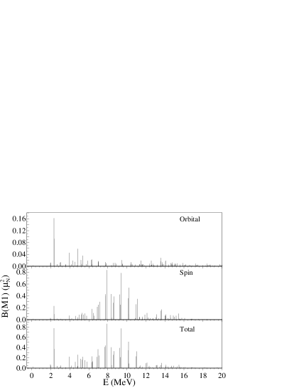
FIG. 8.: $M1$ strength functions of ⁴⁷Ti, using bare gyromagnetic factors. 60 Lanczos iterations for each $J$

FIG. 9.: ⁴⁷Sc$(\beta^{-}){}^{47}$Ti and ⁴⁷Fe$(\beta^{+}){}^{47}$Mn strength function.

FIG. 10.: ⁴⁷Ti$(p,n){}^{47}$V and ⁴⁷Ti$(n,p){}^{47}$Sc strength functions.

FIG. 11.: ⁴⁹Ti$(p,n){}^{49}$V and ⁴⁹Ti$(n,p){}^{49}$Sc strength functions.

FIG. 12.: Theoretical levels for the KB, KB’ and KB3 interactions compared with experiment in ⁴⁹Ca.

FIG. 13.: Theoretical and experimental energy levels of ⁴⁹Sc.

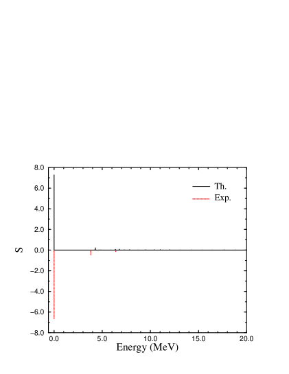
FIG. 14.: Spectroscopic factors, $(2j+1)S(j,t_{z})$, corresponding to stripping of a particle in the orbit 1$f_{7/2}$.

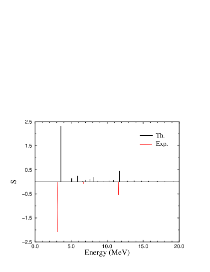
FIG. 15.: Spectroscopic factors, $(2j+1)S(j,t_{z})$, corresponding to stripping of a particle in the orbit 0$p_{3/2}$.

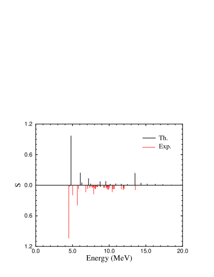
FIG. 16.: Spectroscopic factors, $(2j+1)S(j,t_{z})$, corresponding to stripping of a particle in the orbit 0$p_{1/2}$.

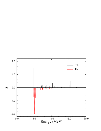
FIG. 17.: Spectroscopic factors, $(2j+1)S(j,t_{z})$, corresponding to stripping of a particle in the orbit 1$f_{5/2}$.

FIG. 18.: Experimental excitation energies of ⁴⁷Ti compared with a rotational spectrum.

FIG. 19.: Comparison between the spectrum of ⁴⁷V and ⁴⁹Cr and the predictions of the rotational model. For ⁴⁷V we use the experimental energies measured in [19] with the energies of the 17/2 and 21/2 taken from the mirror nucleus ⁴⁷Cr. For ⁴⁹Cr we use the theoretical energies because of the discrepancies noted in section II C

FIG. 20.: Gyromagnetics factors of ⁴⁸Cr and its comparison with the isoscalar part of the gyromagnetic factors of the mirror pairs ⁴⁷V-⁴⁷Cr and ⁴⁹Cr-⁴⁹Mn.

FIG. 21.: Gyromagnetics factors of the nuclei ⁴⁷V, ⁴⁷Cr, ⁴⁹Cr and ⁴⁹Mn as a function of the angular momentum. The curves represent the predictions of the particle plus rotor model.

FIG. 22.: Nilsson orbits for SU(3) and quasi-SU(3). The band heads are at $-2p=-6$ for SU(3) and $-2p+1/2=-11/2$ for quasi-SU(3).

FIG. 23.: Nilsson diagrams in the $pf$ shell. Energy vs. single particle splitting $\varepsilon$ (left panel), energy vs. deformation $\delta$ (right panel).

TABLE I.: $m$-scheme and maximal $JT$ dimensions in the full $pf$ shell.

	47Ca	47Sc	47Ti	47V
$m$-scheme	7 531	71 351	262 231	483 887
$2J\ 2T$	7 7	9 5	9 3	9 1
	1 121	8 858	25 600	29 121
	49Ca	49Sc	49Ti	49V	49Cr
$m$-scheme	15 666	219 781	1 227 767	3 580 369	6 004 205
$2J\ 2T$	7 9	9 7	9 5	9 3	9 1
	2 215	27 091	127 406	287 309	289 959

TABLE II.: Dipole magnetic moments and quadrupole electric moments of the $A=47$ isobars.

Nucleus	State	$\mu$ ($\mu_{N}$)		$Q$ ($e$ fm2)
		Expt.	Theor.	Expt.	Theor.
47Ca	7/2- (g.s.)	$-$1.380(24)	$-$1.41	2.1(4)	6.7
47Sc	7/2- (g.s.)	5.34(2)	5.12	$-$22(3)	$-$21
47Ti	5/2- (g.s.)	$-$0.78848(1)	$-$0.97	30.3(24)	22.7
	5/2-	$-$1.9(6)	$-$1.16		8.16
47V	3/2- (g.s.)		2.14		19.9
47Cr	3/2- (g.s.)		$-$0.47		20.6

TABLE III.: $E2$ and $M1$ transitions of ⁴⁷Sc.

$J^{\pi}_{n}$(i)	$J^{\pi}_{m}$(f)	$B(E2)$ ($e^{2}$ fm4)		$B(M1)$ ($\mu_{N}^{2}$)
		Expt.	Theor.	Expt.	Theor.
$\frac{3}{2}^{-}_{1}$	$\frac{7}{2}^{-}_{1}$	111(30)	60
$\frac{11}{2}^{-}_{1}$	$\frac{7}{2}^{-}_{1}$	91(30)	24
$\frac{5}{2}^{-}_{1}$	$\frac{3}{2}^{-}_{1}$	1108(605)	38	0.41(14)	1.82
$\frac{5}{2}^{-}_{1}$	$\frac{7}{2}^{-}_{1}$	0.9${}^{+1.5}_{-0.9}$	0.48	0.27(9)	0.66
$\frac{9}{2}^{-}_{1}$	$\frac{11}{2}^{-}_{1}$	130${}^{+220}_{-130}$	6.3	0.25(14)	1.72
$\frac{9}{2}^{-}_{1}$	$\frac{7}{2}^{-}_{1}$	3${}^{+4}_{-3}$	9.2	0.034(18)	0.25
$\frac{7}{2}^{-}_{2}$	$\frac{5}{2}^{-}_{1}$			$>0.077$	1.17
$\frac{5}{2}^{-}_{2}$	$\frac{3}{2}^{-}_{1}$			$>0.016$	0.021

TABLE IV.: $E2$ and $M1$ transitions of ⁴⁷Ti.

$J^{\pi}_{n}$(i)	$J^{\pi}_{m}$(f)	$B(E2)$ ($e^{2}$ fm4)		$B(M1)$ ($\mu_{N}^{2}$)
		Expt.	Theor.	Expt.	Theor.
$\frac{7}{2}^{-}_{1}$	$\frac{5}{2}^{-}_{1}$	252(50)	140	0.0460(14)	0.0175
$\frac{9}{2}^{-}_{1}$	$\frac{7}{2}^{-}_{1}$	191(40)	102	0.188(20)	0.154
$\frac{9}{2}^{-}_{1}$	$\frac{5}{2}^{-}_{1}$	70(30)	55
$\frac{11}{2}^{-}_{1}$	$\frac{9}{2}^{-}_{1}$	705(605)	83	0.70(13)	0.242
$\frac{11}{2}^{-}_{1}$	$\frac{7}{2}^{-}_{1}$	159(25)	98
$\frac{3}{2}^{-}_{1}$	$\frac{7}{2}^{-}_{1}$	39(11)	46
$\frac{3}{2}^{-}_{1}$	$\frac{5}{2}^{-}_{1}$	3.3(15)	22	0.00270(90)	0.00011
$\frac{1}{2}^{-}_{1}$	$\frac{5}{2}^{-}_{1}$	$<17$	21
$\frac{3}{2}^{-}_{2}$	$\frac{7}{2}^{-}_{1}$	36.3(70)	8.3
$\frac{3}{2}^{-}_{2}$	$\frac{5}{2}^{-}_{1}$	$<272$	0.48	0.0734(125)	0.102
$\frac{15}{2}^{-}_{1}$	$\frac{11}{2}^{-}_{1}$	135(26)	111
$\frac{17}{2}^{-}_{1}$	$\frac{15}{2}^{-}_{1}$	604${}^{+70}_{-604}$	41	1.02(32)	0.793
$\frac{19}{2}^{-}_{1}$	$\frac{17}{2}^{-}_{1}$	$<50$	25	0.45(13)	1.03

TABLE V.: $E2$ and $M1$ transitions of ⁴⁷V.

$J^{\pi}_{n}$(i)	$J^{\pi}_{m}$(f)	$B(E2)$ ($e^{2}$ fm4)		$B(M1)$ ($\mu_{N}^{2}$)
		Expt.	Theor.	Expt.	Theor.
$\frac{5}{2}^{-}_{1}$	$\frac{3}{2}^{-}_{1}$	2418(806)	251	0.082(5)	0.125
$\frac{7}{2}^{-}_{1}$	$\frac{5}{2}^{-}_{1}$			0.354(43)	0.239
$\frac{7}{2}^{-}_{1}$	$\frac{3}{2}^{-}_{1}$	91(71)	106
$\frac{9}{2}^{-}_{1}$	$\frac{7}{2}^{-}_{1}$	$161<B(E2)<1300$	76	$0.0023<B(M1)<0.12$	0.080
$\frac{9}{2}^{-}_{1}$	$\frac{5}{2}^{-}_{1}$	181(60)	138
$\frac{11}{2}^{-}_{1}$	$\frac{7}{2}^{-}_{1}$	201(101)	186

TABLE VI.: Dipole magnetic moments and quadrupole electric moments of the $A=49$ isobars.

Nucleus	State	$\mu$ ($\mu_{N}$)		$Q$ ($e$ fm2)
		Expt.	Theor.	Expt.	Theor.
49Ca	3/2- (g.s.)	$-$1.38(6)	$-$1.46		$-$3.95
49Sc	7/2- (g.s.)		5.38		$-$19.3
49Ti	7/2- (g.s.)	$-$1.10417(1)	$-$1.12	24(1)	22
49V	7/2- (g.s.)	$\pm$4.47(5)	4.37		$-$11.1
	3/2- (0.153)	2.37(12)	2.25		18.87
49Cr	5/2- (g.s.)	$\pm$0.476(3)	$-$0.50		36.1
	19/2- (4.365)	7.4(12)	6.28		$-3.43$
49Mn	5/2- (g.s.)		$-$3.24		36.4

TABLE VII.: $E2$ and $M1$ transitions in ⁴⁹Ti. The identification of the states follows the theoretical results.

$J^{\pi}_{n}$(i)	$J^{\pi}_{m}$(f)	$B(E2)$ ($e^{2}$ fm4)		$B(M1)$ ($\mu_{N}^{2}$)
		Expt.	Theor.	Expt.	Theor.
$\frac{3}{2}^{-}_{1}$	$\frac{7}{2}^{-}_{1}$	33(4)	26
$\frac{11}{2}^{-}_{1}$	$\frac{7}{2}^{-}_{1}$	65(6)	72
$\frac{3}{2}^{-}_{2}$	$\frac{7}{2}^{-}_{1}$	$7.42<B(E2)<10.3$	54
$\frac{9}{2}^{-}_{1}$	$\frac{7}{2}^{-}_{1}$	$<1.49\times 10^{3}$	101	$<0.29$	0.24
$\frac{1}{2}^{-}_{1}$	$\frac{3}{2}^{-}_{1}$	$0.17<B(E2)<3.37\times 10^{3}$	125	$1.39\times 10^{-4}<B(M1)<2.72$	0.52
$\frac{1}{2}^{-}_{1}$	$\frac{3}{2}^{-}_{2}$	$32<B(E2)<7.0\times 10^{5}$	68	$<0.93$	0.17
$\frac{5}{2}^{-}_{1}$	$\frac{7}{2}^{-}_{1}$	$11<B(E2)<202$	56	$0.20<B(M1)<0.32$	0.31
$\frac{7}{2}^{-}_{2}$	$\frac{5}{2}^{-}_{1}$			0.88(27)	0.79
$\frac{7}{2}^{-}_{2}$	$\frac{9}{2}^{-}_{1}$			0.98(45)	1.07
$\frac{7}{2}^{-}_{2}$	$\frac{7}{2}^{-}_{1}$	$<73$	18	$<0.27$	0.0096
$\frac{7}{2}^{-}_{3}$	$\frac{5}{2}^{-}_{1}$			0.38(18)	0.71
$\frac{7}{2}^{-}_{3}$	$\frac{9}{2}^{-}_{1}$			0.48(23)	0.97
$\frac{7}{2}^{-}_{3}$	$\frac{7}{2}^{-}_{1}$	$<50$	11	$<0.021$	0.012
$\frac{15}{2}^{-}_{1}$	$\frac{11}{2}^{-}_{1}$	$0.099<B(E2)<195$	46
$\frac{17}{2}^{-}_{1}$	$\frac{15}{2}^{-}_{1}$	$>270$	49	$>1.15$	1.74

TABLE VIII.: $E2$ and $M1$ transitions in ⁴⁹V.

$J^{\pi}_{n}$(i)	$J^{\pi}_{m}$(f)	$B(E2)$ ($e^{2}$ fm4)		$B(M1)$ ($\mu_{N}^{2}$)
		Expt.	Theor.	Expt.	Theor.
$\frac{5}{2}^{-}_{1}$	$\frac{7}{2}^{-}_{1}$			0.224(14)	0.12
$\frac{3}{2}^{-}_{1}$	$\frac{5}{2}^{-}_{1}$			0.00267(9)	0.0028
$\frac{3}{2}^{-}_{1}$	$\frac{7}{2}^{-}_{1}$	204(6)	196
$\frac{11}{2}^{-}_{1}$	$\frac{7}{2}^{-}_{1}$	149(27)	157
$\frac{9}{2}^{-}_{1}$	$\frac{11}{2}^{-}_{1}$			0.41(18)	0.50
$\frac{9}{2}^{-}_{1}$	$\frac{5}{2}^{-}_{1}$	84(24)	88
$\frac{9}{2}^{-}_{1}$	$\frac{7}{2}^{-}_{1}$	63(19)	41	0.0120(34)	0.0066
$\frac{15}{2}^{-}_{1}$	$\frac{11}{2}^{-}_{1}$	298${}^{+85}_{-180}$	140
$\frac{11}{2}^{-}_{2}$	$\frac{11}{2}^{-}_{1}$	$>460$	0.46	$>0.66$	0.72
$\frac{15}{2}^{-}_{2}$	$\frac{15}{2}^{-}_{1}$	$<1.28(53)\times 10^{3}$	99	2.0(9)	1.40
$\frac{15}{2}^{-}_{2}$	$\frac{11}{2}^{-}_{1}$	190(90)	34
$\frac{13}{2}^{-}_{1}$	$\frac{15}{2}^{-}_{1}$			0.39(30)	1.0
$\frac{13}{2}^{-}_{1}$	$\frac{9}{2}^{-}_{1}$	290(200)	110

TABLE IX.: $E2$ and $M1$ transitions in ⁴⁹Cr.

$J^{\pi}_{n}$(i)	$J^{\pi}_{m}$(f)	$B(E2)$ ($e^{2}$ fm4)		$B(M1)$ ($\mu_{N}^{2}$)
		Expt.	Theor.	Expt.	Theor.
$\frac{7}{2}^{-}_{1}$	$\frac{5}{2}^{-}_{1}$	383(117)	332	0.15(4)	0.14
$\frac{9}{2}^{-}_{1}$	$\frac{7}{2}^{-}_{1}$	426(149)	283	0.45(9)	0.39
$\frac{9}{2}^{-}_{1}$	$\frac{5}{2}^{-}_{1}$	149(43)	97
$\frac{11}{2}^{-}_{1}$	$\frac{9}{2}^{-}_{1}$	107(85)	213	0.50(9)	0.47
$\frac{11}{2}^{-}_{1}$	$\frac{7}{2}^{-}_{1}$	213(43)	166
$\frac{1}{2}^{-}_{1}$	$\frac{5}{2}^{-}_{1}$	$<10$	7.0
$\frac{3}{2}^{-}_{1}$	$\frac{7}{2}^{-}_{1}$	21(6)	4.1
$\frac{3}{2}^{-}_{1}$	$\frac{5}{2}^{-}_{1}$	0.26(12)	4.8	0.0048(14)	0.00003
$\frac{13}{2}^{-}_{1}$	$\frac{11}{2}^{-}_{1}$	$4^{+106}_{-4}$	153	0.27(7)	0.62
$\frac{13}{2}^{-}_{1}$	$\frac{9}{2}^{-}_{1}$	64(30)	192
$\frac{15}{2}^{-}_{1}$	$\frac{13}{2}^{-}_{1}$	$<256$	92	0.20(7)	0.79
$\frac{15}{2}^{-}_{1}$	$\frac{11}{2}^{-}_{1}$	92(27)	185
$\frac{19}{2}^{-}_{1}$	$\frac{17}{2}^{-}_{1}$			0.356(32)	0.520
$\frac{19}{2}^{-}_{1}$	$\frac{15}{2}^{-}_{1}$	127(10)	158

TABLE X.: $S_{+}$ strength for $t=1$ and full calculations. $\overline{q}$ is the average of the ratios between the two values of the strength for a given $Z$

Nucleus	Space	$A=47$	$A=48$	$A=49$	$\overline{q}$
Sc	$t=1$	1.72	1.71	1.71	1.96
	full	0.89	0.85	0.88
Ti	$t=1$	3.45	3.44	3.43	2.60
	full	1.39	1.26	1.33
V	$t=1$	5.58	5.23	5.16	1.88
	full	2.94	2.87	2.67
Cr	$t=1$		7.66	7.24	1.80
	full		4.13	4.13

TABLE XI.: Experimental and theoretical half-lives using the quenching factor 0.77.

Nucleus	Half-Life		Fermi (%)
	Expt.	Theor.	Expt.	Theor.
47Ca	4.336(3) d	4.20 d
47Sc	3.3492(6) d	3.79 d
47V	36.6(3) m	20.7 m
47Cr	500(15) ms	480 ms	78.7	76.1
47Mn		65.2 ms		54.1
47Fe		18.7 ms		26

TABLE XII.: Experimental and theoretical half-lifes using the quenching factor 0.77

Nucleus	Half-Life		Fermi (%)
	Expt.	Theor.	Expt.	Theor.
49Ca	8.718(6) m	3.17 m
49Sc	57.2(2) m	41.4 m
49V	330(15) d	1088 d
49Cr	42.3(1) m	38.2 m
49Mn	382(7) ms	398 ms	72	75
49Fe	75(10)	55 ms	61	42

TABLE XIII.: Binding energies (in MeV) of the $A=47$ nuclei relative to ⁴⁰Ca. The experimental values are from reference [37]. Asterisks are used for those obtained from systematics.

	Ca	Sc	Ti	V	Cr	$Mn$	$Fe$
Expt.	63.99	65.20	65.02	61.31	53.08	$40.01^{*}$	$23.58^{*}$
Theor.	64.06	65.11	64.81	61.07	52.89	$40.28$	$24.22$

TABLE XIV.: Binding energies (in MeV) of the $A=49$ nuclei relative to ⁴⁰Ca. The experimental values are from reference [37]. Asterisks are used for those obtained from systematics.

	Ca	Sc	Ti	V	Cr	Mn	$Fe$	$Co$
Expt.	79.09	83.57	84.79	83.40	79.99	71.50	$57.69^{*}$	$42.20^{*}$
Theor.	78.75	83.69	85.12	83.70	80.23	71.75	$58.27$	$42.73$

TABLE XV.: Intrinsic quadrupole moments ($e$ fm²) of ⁴⁷Ti. The numbers in parenthesis have been calculated using the experimental data. $Q_{0}^{(s)}$ means computed from the spectroscopic moment. $Q_{0}^{(t)}$ from the $B(E2)$ value.

$J$	$Q_{0}^{(s)}$	$Q_{0}^{(t)}$
		$\Delta J=1$	$\Delta J=2$
$5/2^{-}$	63.4 (84.8)
$7/2^{-}$	120.3	61.6 (84.2)
$9/2^{-}$	44.1	57.1 (79.6)	72.7 (83.9)
$11/2^{-}$	10.9	58.6	74.7 (97.1)
$13/2^{-}$	60.7	57.3	67.5
$15/2^{-}$	29.8	50.2	66.0 (74.1)
$17/2^{-}$	69.7	59.3	59.7
$19/2^{-}$	45.6	50.6	51.9
$21/2^{-}$	66.6	40.3	40.4
$23/2^{-}$	53.5	56.8	43.1
$25/2^{-}$	30.1	9.1	20.3
$27/2^{-}$	46.7	65.8	28.8

TABLE XVI.: Intrinsic quadrupole moments ($e$ fm²) of the mirror pair ⁴⁷V-⁴⁷Cr. The numbers in parenthesis have been calculated using the experimental data. $Q_{0}^{(s)}$ means computed from the spectroscopic moment. $Q_{0}^{(t)}$ from the $B(E2)$ value. When a state can decay to two, both numbers are given.

	47V			47Cr
$J^{\pi}_{n}$	$Q_{0}^{(s)}$	$Q_{0}^{(t)}$		$Q_{0}^{(s)}$	$Q_{0}^{(t)}$
		$\Delta J=1$	$\Delta J=2$		$\Delta J=1$	$\Delta J=2$
$3/2^{-}$	100			103
$5/2^{-}$	138	87 (266)		143	95
$7/2^{-}$	67	99	88 (80)	85	102	95
$9/2^{-}$	101	75	82 (92)	105	87	95
$11/2^{-}$	69	100	87 (89)	84	102	98
$13/2^{-}$	101	66	77	106	80	87
$15/2^{-}$	69	103	81	83	105	91
$17/2^{-}_{1}$	$-5.5$	22	17	2.7	35	18
$17/2^{-}_{2}$	68	41	66	63	57	71
$19/2^{-}$	39	106, 109	65	41	88, 122	73
$21/2^{-}$	38	35	54, 39.6	37	5.4	53, 42
$23/2^{-}$	42	43	66	41	26	69
$25/2^{-}$	45	53	57	40	8.4	59
$27/2^{-}$	38	63	55	28	66	55
$29/2^{-}$	35	22	32	29	13	40
$31/2^{-}$	42	69	41	30	29	48

TABLE XVII.: Intrinsic quadrupole moments ($e$ fm²) of the mirror pair ⁴⁹Cr-⁴⁹Mn. The numbers in parenthesis have been calculated using the experimental data. $Q_{0}^{(s)}$ means computed from the spectroscopic moment. $Q_{0}^{(t)}$ from the $B(E2)$ value. When a state can decay to two, both numbers are given.

	49Cr			49Mn
$J^{\pi}_{n}$	$Q_{0}^{(s)}$	$Q_{0}^{(t)}$		$Q_{0}^{(s)}$	$Q_{0}^{(t)}$
		$\Delta J=1$	$\Delta J=2$		$\Delta J=1$	$\Delta J=2$
$5/2^{-}$	101			102
$7/2^{-}$	142	98 (104)		114	101
$9/2^{-}$	92	98 (119)	100 (122)	102	95	101
$11/2^{-}$	69	97	101 (112)	73	97	102
$13/2^{-}$	98	94	96 (55)	98	87	95
$15/2^{-}$	47	82	88 (61)	39	86	85
$17/2^{-}$	34	72	75	40	74	74
$19/2^{-}_{1}$	9.8	87	76 (67)	4.5	105	74
$19/2^{-}_{2}$	50	17	37	37	4.1	40
$21/2^{-}$	29	67, 30	66	39	76, 32	68
$23/2^{-}$	13	87	68, 14	9.0	112	72, 6.7
$25/2^{-}$	$-39$	8.6	17	$-44$	8.4	22
$27/2^{-}$	$-5.1$	50	52	$-16$	34	55
$29/2^{-}$	$-1.4$	35	43	$-18$	12	33
$31/2^{-}$	$-4.6$	28	42	$-24$	33	37

REFERENCES

- [1] E. Caurier, A. P. Zuker, A. Poves, and G. Martínez-Pinedo, Phys. Rev. C 50, 225 (1994).
- [2] E. Caurier, A. Poves and A. P. Zuker, Phys. Rev. Lett. 74, 1517 (1995).
- [3] E. Caurier, G. Martínez-Pinedo, A. Poves and A. P. Zuker, Phys. Rev. C 52, R1736 (1995).
- [4] J. A. Cameron, M. A. Bentley, A. M. Bruce, R. A. Cunningham, H. G. Price, J. Simpson, D. D. Warner, A. N. James, W. Gelletly and P. Van Isacker, Phys. Lett. 319B, 58 (1993).
- [5] E. Caurier, J. L. Egido, G. Martínez-Pinedo, A. Poves, J. Retamosa, L. M. Robledo and A. P. Zuker, Phys. Rev. Lett. 75, 2466 (1995).
- [6] G. Martínez-Pinedo, A. Poves, L. M. Robledo, E. Caurier, F. Nowacki, and A. P. Zuker, submitted to Phys. Rev. C, LANL archive nucl-th/9604039.
- [7] S. Lenzi. et al., Z. PhysA354, 117 (1996), and private communications from S. Lenzi and J. Cameron.
- [8] T. W. Burrows, Nucl. Data Sheets, 74, 1 (1995).
- [9] T. W. Burrows, Nucl. Data Sheets, 76, 191 (1995); 48, 569 (1986).
-
[10]
Electronic version of Nuclear Data Sheets,
telnet://bnlnd2.dne.bnl.gov (130.199.112.132),
http://www.dne.bnl.gov/nndc.html. - [11] T. T. S. Kuo and G. E. Brown, Nucl. Phys. A114, 235 (1968).
- [12] E. Pasquini, Ph. D. thesis, Report No. CRN/PT 76-14, Strasburg, 1976.
- [13] E. Pasquini and A. P. Zuker in Physics of Medium Light Nuclei, Florence, 1977, edited by P. Blasi and R. Ricci (Editrice Compositrice, Bologna, 1978).
- [14] A. Poves, E. Pasquini and A. P. Zuker, Phys. Lett. 82B, 319 (1979).
- [15] A. Poves and A. P. Zuker, Phys. Rep. 70, 235 (1981).
- [16] A. Zuker, J. Retamosa, A. Poves and E. Caurier, Phys. Rev. C52, R1742 (1995).
- [17] E. Caurier, computer code ANTOINE, CRN, Strasburg, 1989.
- [18] E. Caurier, A. Poves and A. P. Zuker, in Nuclear Structure of Light Nuclei far from Stability. Experiment and Theory, proceedings of the Workshop, Obernai, edited by G. Klotz, (CRN, Strasburg, 1989).
- [19] J. A. Cameron, M. A. Bentley, A. M. Bruce, R. A. Cunningham, W. Gelletly, H. G. Price, J. Simpson, D. D. Warner, and A. N. James, Phys. Rev. C 49, 1347 (1994).
- [20] J. A. Cameron, M. A. Bentley, A. M. Bruce, R. A. Cunningham, W. Gelletly, H. G. Price, J. Simpson, D. D. Warner, and A. N. James, Phys. Rev. C 44, 1882 (1991).
- [21] J. D. McCullen, B. F. Bayman, and L. Zamick, Phys. Rev. 4, B515 (1964).
- [22] R. R. Whitehead, in Moment methods in many fermion systems, edited by B. J. Dalton et al. (Plenum, New York, 1980).
- [23] E. Caurier, A. Poves and A. P. Zuker, Phys. Lett. 256B, 301 (1991).
- [24] E. Caurier, A. Poves and A. P. Zuker, Phys. Lett. 252B, 13 (1990).
- [25] S. D. Bloom and G. M. Fuller, Nucl. Phys. A440, 511 (1985).
- [26] A. R. Edmonds, Angular Momentum in Quantum Mechanics (Princeton, New Jersey, 1960).
- [27] I. S. Towner, The Nucleus as a Laboratory for Studying Symmetries and Fundamental Interaction, ed. by E. M. Henley and W. C. Haxton, to be published, nucl-th/9504015.
- [28] D. H. Wilkinson and B. E. F. Macefield, Nucl. Phys. A232, 58 (1974).
- [29] W. Bambynek, H. Behrens, M. H. Chen, B. Graseman, M. L. Fitzpatrick, K. W. D. Ledingham, H. Genz, M. Mutterer and R. L. Intemann, Rev. Mod. Phys. 49, 77 (1977).
- [30] D. G. Fleming, O. Nathan, H. B. Jensen and O. Hansen, Phys. Rev. C 5, 1365 (1972).
- [31] P. Raghavan, At. Data Nucl. Data Tables 42, 189 (1989).
- [32] A. Richter, Proc. Int. Summer School, La Rabida, Lectures notes on Physics, Springer 1995.
- [33] H. Liu and L. Zamick, Phys. Rev. C 36, 2057 (1987).
- [34] J.B. French in Isospin in Nuclear Physics (D.H. Wilkinson ed. North-Holland, 1969)
- [35] W. E. Ormand and B. A. Brown, Phys. Rev. C 52, 2455 (1995).
- [36] J. Duflo and A. P. Zuker, in preparation.
- [37] G. Audi and A. H. Wapstra, Nucl. Phys. A565, 1 (1993).
- [38] A. Bohr and B. R. Mottelson, Nuclear Structure, Vol. II (Benjamin, New York, 1975).
- [39] J. P. Elliott, Proc. R. Soc. London 245, 128,562 (1956)
- [40] M. Dufour et A.P. Zuker, to appear in Phys. Rev.C, LANL archive nucl-th/9505010.