A Chiral Effective Lagrangian For Nuclei

Abstract

An effective hadronic lagrangian consistent with the symmetries of quantum chromodynamics and intended for applications to finite-density systems is constructed. The degrees of freedom are (valence) nucleons, pions, and the low-lying non-Goldstone bosons, which account for the intermediate-range nucleon–nucleon interactions and conveniently describe the nonvanishing expectation values of nucleon bilinears. Chiral symmetry is realized nonlinearly, with a light scalar meson included as a chiral singlet to describe the mid-range nucleon–nucleon attraction. The low-energy electromagnetic structure of the nucleon is described within the theory using vector-meson dominance, so that external form factors are not needed. The effective lagrangian is expanded in powers of the fields and their derivatives, with the terms organized using Georgi’s “naive dimensional analysis”. Results are presented for finite nuclei and nuclear matter at one-baryon-loop order, using the single-nucleon structure determined within the model. Parameters obtained from fits to nuclear properties show that naive dimensional analysis is a useful principle and that a truncation of the effective lagrangian at the first few powers of the fields and their derivatives is justified.

I Introduction

Quantum chromodynamics (QCD) is generally accepted as the underlying theory of the strong interaction. At low energies relevant to nuclear physics, however, nucleons and mesons are convenient and efficient degrees of freedom. In particular, relativistic field theories of hadrons, called quantum hadrodynamics (QHD), have been quite successful in describing the bulk and single-particle properties of nuclei and nuclear matter in the mean-field and Dirac–Brueckner–Hartree–Fock approximations[1, 2].

QHD studies based on renormalizable models, however, have encountered difficulties due to large effects from loop integrals that incorporate the dynamics of the quantum vacuum[3, 4, 5]. On the other hand, the “modern” approach to renormalization [6, 7, 8, 9, 10], which makes sense of effective, “cutoff” theories with low-energy, composite degrees of freedom, provides an alternative. When composite degrees of freedom are used, the structure of the particles is described with increasing detail by including more and more nonrenormalizable interactions in a derivative expansion[6]. We seek to merge the successful phenomenology of the QHD approach to nuclei with the modern viewpoint of effective field theories.

The present work is an extension of Refs. [11, 12, 13], which explored some aspects of incorporating QCD symmetries into effective hadronic models. Here we build a more complete effective lagrangian and apply it to nuclei at the one-baryon-loop level. Our two main goals are to include effects of compositeness, such as single-nucleon electromagnetic structure, in a unified, self-consistent framework and to test whether “naive dimensional analysis” (NDA) and naturalness (see below) are useful concepts for effective field theories of nuclei. Eventually, we will need to demonstrate a systematic expansion scheme that includes corrections beyond one-loop order. Nevertheless, Ref. [13] describes how a general energy functional with classical meson fields can implicitly incorporate higher-order contributions. We therefore expect that higher-order many-body effects can be absorbed into the coefficients of our one-loop energy functional when we determine parameters by fitting to nuclear observables. We return to this point later in this section.

Important physical constraints on the effective lagrangian are established by maintaining the symmetries of QCD. These include Lorentz invariance, parity invariance, electromagnetic gauge invariance, isospin, and chiral symmetry. These symmetries constrain the lagrangian most directly by restricting the form of possible interaction terms. In some cases, the magnitude of (or relations between) parameters may also be restricted.

Chiral symmetry has been known to play an important role in hadronic physics at low energies since the early days of current algebra [14, 15]; it is exploited systematically in terms of effective fields in the framework known as chiral perturbation theory (ChPT)[16, 17, 18]. There is also a long history of attempts to unite relativistic mean-field phenomenology based on hadrons with manifest chiral symmetry. In particular, it has been tempting to build upon the linear sigma model [19, 20, 21], with a light scalar meson playing a dual role as the chiral partner of the pion and the mediator of the intermediate-range nucleon–nucleon (NN) attraction. The generic failure of this type of model has been shown in Refs. [11, 13]. However, a light scalar is completely consistent with a nonlinear realization of chiral symmetry [12, 13]. Moreover, in a nonlinear realization, one need not assume that the hadrons are grouped into particular chiral multiplets [24].

The phenomenological success of ChPT establishes the dominant contributions of the vector resonances to the low-energy constants in the pion sector[25, 26, 27]. In particular, a tree-level effective lagrangian with vector mesons is found to be essentially equivalent to ChPT at one-meson-loop order. In the baryon sector, a satisfactory description of the nucleon form factors from vector-meson dominance (VMD) [28, 29, 30] alone has not been found[31]. However, we can describe the long-range parts of the single-nucleon form factors (that is, magnetic moments and mean-square radii) using an effective lagrangian that includes vector mesons and direct couplings of photons to nucleons. Our approach is analogous to that implemented long ago in Ref. [32].

In virtually all previous QHD calculations of finite nuclei, the single-nucleon electromagnetic structure was incorporated “by hand.” After the nuclear structure calculation was completed and “point-nucleon” densities were obtained, they were convoluted with empirical single-nucleon form factors to compute the charge density. The results were typically insensitive to the nature of the form factor, as long as the nucleon charge radius was accurate. In the present work, we do not need external form factors. The large oscillations in the point-nucleon charge density of a nucleus are significantly reduced by virtual mesons inherent in the model, and the low-momentum parts of the charge form factors of various nuclei are well reproduced. Thus we have a unified framework.

To achieve a systematic framework for calculating nuclei, however, we must develop an expansion scheme. ChPT is an expansion in powers of small external momenta and the pion mass. Weinberg[33] applies this small-momentum expansion further to a calculation of the $N$-nucleon “effective potential”, defined as the sum of all connected diagrams for the $S$ matrix (in time-ordered perturbation theory) without $N$-nucleon intermediate states. On the other hand, an expansion of the NN interaction kernel in terms of intermediate states of successively shorter range provides a successful and economical way to accurately describe NN scattering data [34]. Here we combine the ideas of the small-momentum expansion and the intermediate-state expansion by including the low-lying non-Goldstone bosons into the low-energy effective lagrangian. These bosons account for the intermediate-range interactions and conveniently describe the nonvanishing expectation values of nuclear bilinears such as $\overline{N}N$ and $\overline{N}\gamma_{\mu}N$.

There are well-defined resonances in the vector channels, and thus it is natural to identify them with fields in the effective lagrangian; in contrast, the dynamics in the scalar channel is more complicated. Numerous calculations[35, 36, 37, 38, 39] show that correlated two-pion exchange leads to a distribution of strength in the isoscalar-scalar channel at center-of-mass pion energies of roughly 500 to 600 MeV, even in the absence of a low-energy resonance. We therefore introduce an isoscalar-scalar meson as an effective degree of freedom to simulate this strong interaction, just like the non-Goldstone bosons in the vector channels. Such a scalar, with a mass of 500 to 600 MeV, is essential in one-boson-exchange models of the NN potential [34] and in relativistic mean-field models of nuclei[1]. We emphasize that at the level of approximation used in this paper, the scalar field can be introduced without loss of generality. (For example, it can be viewed as a way to remove terms with more than two nucleon fields from a general pion-nucleon lagrangian.) A deeper understanding of the NN interaction in the scalar channel is an important pursuit, but is not needed for our purposes here.

We shall expand our effective hadronic lagrangian in powers of the fields and their derivatives, and organize the terms using “naive dimensional analysis” (NDA)[40]. The NDA framework is used to identify the dimensional factors of any term. After these dimensional factors and some appropriate counting factors are extracted, the remaining dimensionless coefficients are all assumed to be of order unity. This is the so-called naturalness assumption. If naturalness is valid, the effective lagrangian can be truncated at a given order with a reasonable bound on the truncation error for physical observables. Thus we have a controlled expansion, at least at the tree level.

Evidently, for an expansion in powers of the fields and their derivatives to be useful, the naturalness assumption must hold. Implicit in this assumption is that all the short-distance physics is incorporated into the coefficients of the effective lagrangian; otherwise, the truncation error will not be reliably given by NDA power counting when loops are included. Thus, just as in ChPT or in heavy-baryon theories, the nucleon vacuum loops and non-Goldstone-boson loops will be “integrated out”, with their effects buried implicitly in the coefficients. Nevertheless, the nucleon and non-Goldstone-boson fields are still needed in the lagrangian to account for the valence nucleons, to treat the mean fields conveniently, and to apply the usual many-body and field-theoretic techniques. Any contributions from vacuum nucleon or non-Goldstone-boson loops that arise in many-body calculations can formally be cancelled by the appropriate counterterms. These cancellations can always be achieved, since all possible interaction terms consistent with the symmetries are already included in the effective lagrangian. On the other hand, long-distance, finite-density effects should be calculated explicitly in a systematic application of the effective lagrangian.

In principle, the naturalness assumption can be verified by deriving the effective lagrangian from QCD. Since this is not yet feasible, one must fit the unknown parameters to experimental data. At finite density, however, the Fermi momentum enters as a new scale. This complicates the situation, because a treatment of the effective lagrangian at the level of classical meson fields and valence nucleons (the Dirac–Hartree approximation) implies that several different physical effects are implicitly contained in the parameters. Not only are short-distance contributions from meson and nucleon vacuum loops absorbed, but long-distance, many-body effects from well-known ladder and ring diagrams are included approximately as well [13]. Thus the usefulness of NDA, the naturalness assumption, and the expansion in powers of the fields and their derivatives requires further examination when these ideas are applied to problems at finite density. It is not obvious that an effective lagrangian with natural coefficients that include only short-distance physics will remain natural in a one-loop calculation that accounts for higher-order many-body effects by adjustments of the coefficients. Here we rely on fits to the properties of finite nuclei to determine whether the coefficients are natural and our expansion of the lagrangian is useful. (Friar and collaborators have recently investigated naturalness as exhibited by a mean-field point-coupling model[42].) An important topic for future study is to include the many-body dynamics explicitly, so as to disentangle it from the short-range and vacuum dynamics already implicit in the parameters of the low-energy effective lagrangian.

The interaction terms of the nucleons and the non-Goldstone bosons can be quite complicated, and different forms have been used in various models in the literature [43, 44, 45]. Some of these models are actually equivalent if one uses the freedom of field redefinitions[46], which leave the on-shell $S$ matrix invariant[47, 48, 49]. We discuss how to take advantage of this freedom to simplify the interaction terms between the nucleons and the non-Goldstone bosons. As a result, the lagrangian can be conveniently written in a “standard form”, in which one mainly has the traditional Yukawa interactions.

The rest of the paper is organized as follows. In Sec. II, we discuss the construction of an effective hadronic lagrangian consistent with chiral symmetry, gauge invariance, and Lorentz and parity invariance. Chiral symmetry is realized in the standard nonlinear form of Callan, Coleman, Wess, and Zumino (CCWZ)[48]. Neutral scalar and vector mesons are introduced to efficiently describe the mid- and short-range parts of the NN interaction, and the role of broken scale invariance in QCD is considered. Georgi’s naive dimensional analysis and field redefinitions are also discussed, with the new feature of off-shell non-Goldstone bosons. In Sec. III, we show how the electromagnetic structure of the pion and the nucleon can be described in the low-energy regime. Applications to nuclear matter and finite nuclei at the Dirac–Hartree level are presented in Sec. IV, and the results are shown in Sec. V. A discussion and summary is given in Sec. VI.

II Constructing the Lagrangian

We begin this section by showing how we implement nonlinear chiral symmetry and electromagnetic gauge invariance using nucleons, Goldstone pions, and non-Goldstone isovector mesons. Next, we discuss the introduction of neutral vector and scalar mesons that are used to provide an efficient description of the short- and mid-range nucleon–nucleon interaction. To use the resulting lagrangian, which in principle has an infinite number of terms, we must have some systematic truncation procedure, and we develop this using the ideas of naive dimensional analysis and naturalness, together with some observations on the sizes of meson mean fields in nuclei.

A Chiral Symmetry

We illustrate a nonlinear realization of chiral symmetry[48] using a system that consists of rho mesons, pions, and nucleons only. We construct a general effective lagrangian that respects chiral symmetry, Lorentz invariance, and parity conservation. The role of vector-meson dominance (VMD) is also discussed. We restrict ourselves to the chiral limit with massless pions and postpone the generalization to a finite pion mass for future study.

The Goldstone pion fields $\pi^{a}(x)$, with $a=1,\,2,\,{\rm and}\,3\,$, form an isovector, which can be considered as the phase of a chiral rotation of the identity matrix in isospin space:

$$\xi{\bf 1}\xi\equiv U(x)=\exp(i\pi(x)/f_{\pi}){\bf 1}\exp(i\pi(x)/f_{\pi})\ .$$ (1)

Here $f_{\pi}\approx 93\,\mbox{MeV}$ is the pion-decay constant and the pion field is compactly written as $\pi(x)\equiv\mathchoice{{\hbox{\boldmath$\displaystyle\pi$}}}{{\hbox{\boldmath$\textstyle\pi$}}}{{\hbox{\boldmath$\scriptstyle\pi$}}}{{\hbox{\boldmath$\scriptscriptstyle\pi$}}}(x)\,\mathchoice{{\hbox{\boldmath$\displaystyle\cdot$}}}{{\hbox{\boldmath$\textstyle\cdot$}}}{{\hbox{\boldmath$\scriptstyle\cdot$}}}{{\hbox{\boldmath$\scriptscriptstyle\cdot$}}}\,{1\over 2}\mathchoice{{\hbox{\boldmath$\displaystyle\tau$}}}{{\hbox{\boldmath$\textstyle\tau$}}}{{\hbox{\boldmath$\scriptstyle\tau$}}}{{\hbox{\boldmath$\scriptscriptstyle\tau$}}}$, with $\tau^{a}$ being Pauli matrices. The matrix $U$ is the standard exponential representation and the “square root” representation in terms of $\xi$ is particularly convenient for including heavy fields in the chiral lagrangian. The isospinor nucleon field is represented by a column matrix

$$N(x)=\left(\,\begin{array}[]{c}p(x)\\ n(x)\end{array}\right)\ ,$$ (2)

where $p(x)$ and $n(x)$ are the proton and neutron fields respectively. The rho fields $\rho^{a}_{\mu}(x)$ also form an isovector; we use the notation $\rho_{\mu}(x)\equiv\mathchoice{{\hbox{\boldmath$\displaystyle\rho$}}}{{\hbox{\boldmath$\textstyle\rho$}}}{{\hbox{\boldmath$\scriptstyle\rho$}}}{{\hbox{\boldmath$\scriptscriptstyle\rho$}}}_{\mu}(x)\,\mathchoice{{\hbox{\boldmath$\displaystyle\cdot$}}}{{\hbox{\boldmath$\textstyle\cdot$}}}{{\hbox{\boldmath$\scriptstyle\cdot$}}}{{\hbox{\boldmath$\scriptscriptstyle\cdot$}}}\,{1\over 2}\mathchoice{{\hbox{\boldmath$\displaystyle\tau$}}}{{\hbox{\boldmath$\textstyle\tau$}}}{{\hbox{\boldmath$\scriptstyle\tau$}}}{{\hbox{\boldmath$\scriptscriptstyle\tau$}}}$. (See Refs. [26, 50, 51] for discussions of the formal equivalence between the vector and the tensor formulations for spin-1 fields.)

Following CCWZ[48], we define a nonlinear realization of the chiral group $SU(2)_{\rm L}\otimes SU(2)_{\rm R}$ such that, for arbitrary global matrices $L\in SU(2)_{\rm L}$ and $R\in SU(2)_{\rm R}$, we have the mapping

$$L\otimes R:\ \ \ (\xi,\rho_{\mu},N)\longrightarrow(\xi^{\prime},\rho^{\prime}_{\mu},N^{\prime})\ ,$$ (3)

where

$$\xi^{\prime}(x) = L\xi(x)h^{\dagger}(x)=h(x)\xi(x)R^{\dagger}\ ,$$ (4)

$$\rho^{\prime}_{\mu}(x) = h(x)\rho_{\mu}(x)h^{\dagger}(x)\ ,$$ (5)

$$N^{\prime}(x) = h(x)N(x)\ .$$ (6)

As usual, the matrix $U$ transforms as $U^{\prime}(x)=LU(x)R^{\dagger}$. The second equality in Eq. (4) defines $h(x)$ implicitly as a function of $L$, $R$, and the local pion fields: $h(x)=h(\mathchoice{{\hbox{\boldmath$\displaystyle\pi$}}}{{\hbox{\boldmath$\textstyle\pi$}}}{{\hbox{\boldmath$\scriptstyle\pi$}}}{{\hbox{\boldmath$\scriptscriptstyle\pi$}}}(x),L,R)$. Under parity, which is defined to be

$${\cal P}:\ \ \ L\rightarrow R\ ,\ \ R\rightarrow L\ ,$$ (7)

the pion field transforms as a pseudoscalar: $\xi(t,{\bf x})\rightarrow\xi^{\dagger}(t,{\bf-x})$. The existence of the parity automorphism (7) allows the simple decomposition $U=\xi\xi$ in Eq. (1) [48]. It follows from Eq. (4) that $h(x)$ is invariant under parity, that is, $h(x)\in SU(2)_{\rm V}$, with $SU(2)_{\rm V}$ the unbroken vector subgroup of $SU(2)_{\rm L}\otimes SU(2)_{\rm R}$. Eqs. (5) and (6) ensure that the rho and nucleon transform linearly under $SU(2)_{\rm V}$ in accordance with their isospins. Note that the matrix $h(x)$ becomes global only for $SU(2)_{\rm V}$ transformations, in which case $h=L=R$.

It is straightforward to show that Eqs. (3) to (6) indeed yield a realization of the chiral group [47]. We emphasize that there is no local gauge freedom involved, since there are no arbitrary local gauge functions in the transformations. The nonlinear realization implies that chiral rotations involve the absorption and emission of pions, as expected from a spontaneously broken symmetry[24, 53]. For example, while vector transformations mix the proton with the neutron, axial transformations mix the proton with states of nucleons plus zero-momentum pions.

To complete the building blocks of the chiral effective lagrangian, we define an axial vector field $a_{\mu}(x)$ and a polar vector field $v_{\mu}(x)$ by

$$a_{\mu} \equiv -{i\over 2}(\xi^{\dagger}\partial_{\mu}\xi-\xi\partial_{\mu}\xi^{\dagger})=a_{\mu}^{\dagger}\ ,$$ (8)

$$v_{\mu} \equiv -{i\over 2}(\xi^{\dagger}\partial_{\mu}\xi+\xi\partial_{\mu}\xi^{\dagger})=v_{\mu}^{\dagger}\ ,$$ (9)

both of which contain one derivative. Under a chiral transformation, we find

$$v_{\mu} \rightarrow hv_{\mu}h^{\dagger}-ih\partial_{\mu}h^{\dagger}\ ,$$ (10)

$$a_{\mu} \rightarrow ha_{\mu}h^{\dagger}\ .$$ (11)

Note that to leading order in derivatives,

$$a_{\mu}={1\over f_{\pi}}\partial_{\mu}\pi+\cdots\ ,\ \ \ v_{\mu}=-{i\over 2f_{\pi}^{2}}[\pi,\partial_{\mu}\pi]+\cdots\ .$$ (12)

To maintain chiral invariance, instead of using an ordinary derivative $\partial^{\mu}$ acting on a rho or nucleon field, we should use a covariant derivative $D^{\mu}$. The chirally covariant derivative of the rho field is

$$D_{\mu}\rho_{\nu}=\partial_{\mu}\rho_{\nu}+i[v_{\mu},\rho_{\nu}]\ .$$ (13)

We also define the covariant tensors

$$v_{\mu\nu} = \partial_{\mu}v_{\nu}-\partial_{\nu}v_{\mu}+i[v_{\mu},v_{\nu}]=-i[a_{\mu},a_{\nu}]\ ,$$ (14)

$$\rho_{\mu\nu} = D_{\mu}\rho_{\nu}-D_{\nu}\rho_{\mu}+ig[\rho_{\mu},\rho_{\nu}]\ .$$ (15)

The term proportional to $[\rho_{\mu},\rho_{\nu}]$ on the right-hand side of Eq. (15) vanishes at the mean-field level, so the coupling $g$ will be left unspecified.

To write a general effective lagrangian, we need an organizational scheme for the interaction terms. We organize the lagrangian in increasing powers of the fields and their derivatives. While we do not consistently include loops in this investigation, we assign to each interaction term a size of the order of $k^{\nu}$, with $k$ a generic small momentum, and

$$\nu=d+{n\over 2}+b\ ,$$ (16)

where $d$ is the number of derivatives, $n$ the number of nucleon fields, and $b$ the number of non-Goldstone boson fields in the interaction term. The first two terms in Eq. (16) are suggested by Weinberg’s work [33]. The last term is a generalization that arises because a non-Goldstone boson couples to two nucleon fields. Equation (16) is also consistent with finite-density applications when the density is not too much higher than the nuclear-matter equilibrium density, as we will see in Sec. II.D.

Taking into account chiral symmetry, Lorentz invariance, and parity conservation, we may write the lagrangian through quartic order ($\nu\leq 4$) as

$${\cal L}_{1}(x) = \overline{N}\Big{[}i\gamma^{\mu}(\partial_{\mu}+iv_{\mu}+ig_{\rho}\rho_{\mu})+g_{\rm\scriptscriptstyle A}\gamma^{\mu}\gamma_{5}a_{\mu}-M\Big{]}N$$ (20)

$$-{f_{\rho}g_{\rho}\over 4M}\overline{N}\rho_{\mu\nu}\sigma^{\mu\nu}N-{\kappa_{\pi}\over M}\overline{N}v_{\mu\nu}\sigma^{\mu\nu}N$$

$$-{1\over 2}{\rm tr}(\rho_{\mu\nu}\rho^{\mu\nu})+m_{\rho}^{2}{\rm tr}(\rho_{\mu}\rho^{\mu})-g_{\rho\pi\pi}{2f_{\pi}^{2}\over m_{\rho}^{2}}{\rm tr}\,(\rho_{\mu\nu}v^{\mu\nu})$$

$$+f_{\pi}^{2}{\rm tr}(a_{\mu}a^{\mu})+{4\beta_{\pi}\over M}\overline{N}N{\rm tr}\,(a_{\mu}a^{\mu})+l_{1}[{\rm tr}(a_{\mu}a^{\mu})]^{2}+l_{2}{\rm tr}(v_{\mu\nu}v^{\mu\nu})\ ,$$

where $\sigma_{\mu\nu}=i[\gamma_{\mu},\gamma_{\nu}]/2$, $g_{\rm\scriptscriptstyle A}\approx 1.26$ is the axial coupling constant, $M$ is the nucleon mass, $g_{\rho}$ is the $\rho NN$ coupling, $f_{\rho}$ is the so-called tensor coupling, $g_{\rho\pi\pi}$ is the $\rho\pi\pi$ coupling, and $\beta_{\pi}$, $\kappa_{\pi}$, $l_{1}$, and $l_{2}$ are couplings for higher-order $\pi N$ and $\pi\pi$ interactions. The pion couplings can be determined from $\pi N$ and $\pi\pi$ scattering[18]. We have omitted terms with higher powers of the rho fields, which have small expectation values in finite nuclei, and four- or more-nucleon “contact” terms, which can be represented by appropriate powers of other meson fields, as discussed shortly. A third-order ($\nu=3$) term of the form $\overline{N}N{\rm tr}(\rho_{\mu}\rho^{\mu})$ will be included by coupling a scalar to two rho fields in Sec. II.E. The antisymmetry of rho meson field tensor $\rho_{\mu\nu}$ guarantees three independent degrees of freedom, because there is no momentum conjugate to the time component $\rho_{0}$, and $\rho_{0}$ satisfies an equation of constraint.

Chiral symmetry permits isoscalar-scalar and isoscalar-vector terms like $(\overline{N}N)^{2}$ and $(\overline{N}\gamma_{\mu}N)^{2}$. However, analyses of NN scattering with one-boson exchange potentials [34] shows that the low-lying mesons are sufficient for describing low-energy many-nucleon systems and that they dominate the NN interaction. One may then expect that contact interactions of four (or more) fermions can be removed in favor of couplings to massive non-Goldstone bosons. The following example shows that this should be a good approximation.

Consider an additional isovector-vector contact term $[\overline{N}(\mathchoice{{\hbox{\boldmath$\displaystyle\tau$}}}{{\hbox{\boldmath$\textstyle\tau$}}}{{\hbox{\boldmath$\scriptstyle\tau$}}}{{\hbox{\boldmath$\scriptscriptstyle\tau$}}}/2)\gamma_{\mu}N]^{2}$. The contribution of this term can be absorbed completely into a renormalization of $g_{\rho}$ as follows. If we had constructed ${\cal L}$ by retaining several isovector-vector non-Goldstone bosons, we could eliminate them using their field equations to obtain

$$-{1\over 2}\Big{(}{{{g^{\prime}_{\rho}}}^{2}\over m_{\rho}^{2}}+{g_{1}^{2}\over m_{1}^{2}}+\cdots\Big{)}[\overline{N}(\mathchoice{{\hbox{\boldmath$\displaystyle\tau$}}}{{\hbox{\boldmath$\textstyle\tau$}}}{{\hbox{\boldmath$\scriptstyle\tau$}}}{{\hbox{\boldmath$\scriptscriptstyle\tau$}}}/2)\gamma_{\mu}N]^{2}-{1\over 2}\Big{(}{{g^{\prime}_{\rho}}^{2}\over m_{\rho}^{4}}+{g_{1}^{2}\over m_{1}^{4}}+\cdots\Big{)}\{\partial_{\mu}[\overline{N}(\mathchoice{{\hbox{\boldmath$\displaystyle\tau$}}}{{\hbox{\boldmath$\textstyle\tau$}}}{{\hbox{\boldmath$\scriptstyle\tau$}}}{{\hbox{\boldmath$\scriptscriptstyle\tau$}}}/2)\gamma_{\nu}N]\}^{2}+\cdots\ ,$$ (21)

where $g^{\prime}_{\rho}$ is the $\rho NN$ coupling when the heavier mesons are retained, with couplings to nucleons given by $g_{1}$, … and masses given by $m_{1}$, … . Evidently, the effects of the heavier particles can be absorbed into a redefinition of the $\rho NN$ coupling:

$$g_{\rho}^{2}={g^{\prime}_{\rho}}^{2}+{m_{\rho}^{2}\over m_{1}^{2}}\,g_{1}^{2}+\cdots\ .$$ (22)

If we approximate the second term in Eq. (21) as

$$\Big{(}-{1\over 2}\,{g_{\rho}^{2}\over m_{\rho}^{4}}\Big{)}\{\partial_{\mu}[\overline{N}(\mathchoice{{\hbox{\boldmath$\displaystyle\tau$}}}{{\hbox{\boldmath$\textstyle\tau$}}}{{\hbox{\boldmath$\scriptstyle\tau$}}}{{\hbox{\boldmath$\scriptscriptstyle\tau$}}}/2)\gamma_{\nu}N]\}^{2}\ ,$$ (23)

the leading error is given by the following term:

$${g_{1}^{2}\over g_{\rho}^{2}}\,{m_{\rho}^{2}(m_{1}^{2}-m_{\rho}^{2})\over m_{1}^{4}}\Big{(}-{1\over 2}\,{g_{\rho}^{2}\over m_{\rho}^{4}}\Big{)}\{\partial_{\mu}[\overline{N}(\mathchoice{{\hbox{\boldmath$\displaystyle\tau$}}}{{\hbox{\boldmath$\textstyle\tau$}}}{{\hbox{\boldmath$\scriptstyle\tau$}}}{{\hbox{\boldmath$\scriptscriptstyle\tau$}}}/2)\gamma_{\nu}N]\}^{2}\ .$$ (24)

For a typical resonance in the isovector-vector channel [54], we have $m_{1}=1450\,\mbox{MeV}$ and $m_{\rho}^{2}(m_{1}^{2}-m_{\rho}^{2})/m_{1}^{4}\approx 1/5$. If $g_{1}^{2}/g_{\rho}^{2}$ is roughly $1/4$, the error is about $5\%$ of the already small second term. One should be able to test the sensitivity to these errors by allowing the non-Goldstone boson masses to vary in the fit to nuclear properties.

If we were to assume universal VMD in Eq. (20), then

$$g_{\rho\pi\pi}=g_{\rho}\ ,\qquad\qquad\kappa_{\pi}={f_{\rho}\over 4}\ ,$$ (25)

and $g=g_{\rho}$ in Eq. (15). If we further assume the Kawarabayashi–Suzuki–Riazuddin–Fayyazuddin (KSRF) [55, 56] relation

$$g_{\rho\pi\pi}={m_{\rho}^{2}\over 2g_{\rho}f_{\pi}^{2}}\ ,$$ (26)

then we may redefine the rho field to be $\rho_{\mu}+v_{\mu}/g_{\rho}$ and the covariant field tensor to be $\rho_{\mu\nu}+v_{\mu\nu}/g_{\rho}$, and recover the lagrangian of Weinberg[24] or Bando et al.[57].

B Gauge Invariance and the Inclusion of the $\omega$ Meson

In finite nuclei, electromagnetism also plays an important role. We may include electromagnetic gauge invariance in our formalism in a straightforward manner by noticing how the pion, rho, and nucleon fields transform under the local $U(1)_{Q}$ symmetry. Here the electric charge $Q$, the third component of the isospin $T_{3}$, and the hypercharge $Y$ are related by $Q=T_{3}+Y/2$.

Under $U(1)_{Q}$, the electromagnetic field $A_{\mu}$ transforms in the familiar way

$$A_{\mu}\rightarrow A_{\mu}-{1\over e}\,\partial_{\mu}\alpha(x)\ .$$ (27)

The pion, rho, and nucleon fields transform under the local $U(1)_{Q}$ rotation just as in Eqs. (4) to (6), with both $L$ and $R$ set equal to

$$h(x)=\exp\Big{[}i\alpha(x)\Big{(}{\tau_{3}+Y\over 2}\Big{)}\Big{]}\ ,$$ (28)

where $Y=0$ for the pion and the rho, and $Y=1$ for the nucleon. Indeed, the resulting transformations for these hadrons are just as expected from their electric charges. That is,

$$(\pi^{0},\ \pi^{\pm}) \rightarrow (\pi^{0},\ e^{\pm i\alpha}\pi^{\pm})\ ,$$ (29)

$$(\rho_{\mu}^{0},\ \rho_{\mu}^{\pm}) \rightarrow (\rho_{\mu}^{0},\ e^{\pm i\alpha}\rho_{\mu}^{\pm})\ ,$$ (30)

$$(n,\ p) \rightarrow (n,\ e^{+i\alpha}p)\ .$$ (31)

Electromagnetism breaks chiral symmetry. The lagrangian in Eq. (20) becomes gauge invariant if the ordinary derivatives are replaced with the covariant derivatives

$$\partial_{\mu}\xi \rightarrow \partial_{\mu}\xi+ieA_{\mu}\Bigl{[}{\tau_{3}\over 2},\xi\Bigr{]}\ ,$$ (32)

$$\partial_{\mu}N \rightarrow \Bigl{(}\partial_{\mu}+{i\over 2}eA_{\mu}(1+\tau_{3})\Bigr{)}N\ ,$$ (33)

$$\partial_{\mu}\rho_{\nu} \rightarrow \partial_{\mu}\rho_{\nu}+ieA_{\mu}\Bigl{[}{\tau_{3}\over 2},\rho_{\nu}\Bigr{]}\ .$$ (34)

As a result, the axial and vector pion fields become

$$\widetilde{a}_{\mu} = a_{\mu}+{1\over 2}eA_{\mu}\Big{(}\xi\,[{\tau_{3}\over 2},\xi^{\dagger}]-\xi^{\dagger}\,[{\tau_{3}\over 2},\xi]\Big{)}\ ,$$ (35)

$$\widetilde{v}_{\mu} = v_{\mu}+{1\over 2}eA_{\mu}\Big{(}\xi\,[{\tau_{3}\over 2},\xi^{\dagger}]+\xi^{\dagger}\,[{\tau_{3}\over 2},\xi]\Big{)}\ ,$$ (36)

respectively, and the pion “kinetic” term is

$$f_{\pi}^{2}{\rm tr}\,(\widetilde{a}_{\mu}\widetilde{a}^{\mu})=f_{\pi}^{2}{\rm tr}\,(a_{\mu}a^{\mu})-2ef_{\pi}^{2}A^{\mu}{\rm tr}\,(v_{\mu}\tau_{3})+\cdots\ .$$ (37)

In addition to terms arising from the preceding minimal substitutions, there can be other non-minimal terms in the general effective lagrangian. For example, it is possible to have a direct rho-photon coupling term [58]

$$-{e\over 2g_{\gamma}}F_{\mu\nu}\,{\rm tr}\,(\tau_{3}\widetilde{\rho}^{\mu\nu})\ ,$$ (38)

where $\widetilde{\rho}^{\mu\nu}$ is given by Eq. (15) with the replacements in Eqs. (32) and (34), and $F_{\mu\nu}$ is the usual electromagnetic field tensor. In principle, a similar term proportional to $F_{\mu\nu}\,{\rm tr}\,(\tau_{3}\widetilde{v}^{\mu\nu})$ is also possible, although VMD applied to the pion form factor suggests that the coefficient of this term is small [31]. Furthermore, the photon can couple to the nucleon as

$$-{e\over 4M}F_{\mu\nu}\overline{N}\lambda\sigma^{\mu\nu}N+{e\over 2M^{2}}\partial_{\mu}F^{\mu\nu}\overline{N}\gamma_{\nu}(\beta_{\rm s}+\beta_{\rm v}\tau_{3})N+\cdots\ ,$$ (39)

where

$$\lambda\equiv{1\over 2}\lambda_{\rm p}(1+\tau_{3})+{1\over 2}\lambda_{\rm n}(1-\tau_{3})\ ,$$ (40)

with $\lambda_{\rm p}=1.793$ and $\lambda_{\rm n}=-1.913$ the anomalous magnetic moments of the proton and the neutron, respectively. The first term in Eq. (39) is needed to reproduce the magnetic moments of the nucleons, and the second one contributes to the rms charge radii. Note that these terms have $\nu=3$ and $\nu=4$, respectively.

We may now write down the resulting manifestly gauge-invariant lagrangian, which contains the preceding “tilde” fields. Instead of showing this lagrangian in its entirety, however, we omit terms that are irrelevant to our applications here. The remaining lagrangian is manifestly chiral invariant, except for some terms involving the photon field that are proportional to the electric charge. We find

$${\cal L}_{2}(x) = {\cal L}_{1}(x)-{1\over 2}eA_{\mu}\overline{N}\gamma^{\mu}(1+\tau_{3})N-{e\over 2g_{\gamma}}F_{\mu\nu}\,{\rm tr}\,(\tau_{3}\rho^{\mu\nu})-2ef_{\pi}^{2}A^{\mu}{\rm tr}\,(v_{\mu}\tau_{3})$$ (42)

$$-{e\over 4M}F_{\mu\nu}\overline{N}\lambda\sigma^{\mu\nu}N+{e\over 2M^{2}}\partial_{\mu}F^{\mu\nu}\overline{N}\gamma_{\nu}(\beta_{\rm s}+\beta_{\rm v}\tau_{3})N-{1\over 4}F_{\mu\nu}F^{\mu\nu}\ .$$

It is well known that the isoscalar-vector $\omega$ meson is needed to describe the short-range repulsion of the NN interaction. To have a realistic description of nuclear systems, the $\omega$ meson should be included. Note that once the $\omega$ meson is introduced, an isoscalar-vector four-fermion term $(\overline{N}\gamma_{\mu}N)^{2}$ can be completely accounted for by adjusting $g_{\rm v}$ to fit experimental data, as discussed above for the rho meson.

With respect to chiral $SU(2)$ symmetry, the $\omega$ meson can be treated as a chiral singlet represented by a vector field $V_{\mu}(x)$. The relevant lagrangian can be written as

$${\cal L}_{\rm v}(x) = -{1\over 4}V_{\mu\nu}V^{\mu\nu}+{1\over 2}m_{\rm v}^{2}V_{\mu}V^{\mu}-g_{\rm v}\overline{N}\gamma^{\mu}V_{\mu}N$$ (44)

$$-{f_{\rm v}g_{\rm v}\over 4M}\overline{N}V_{\mu\nu}\sigma^{\mu\nu}N-{e\over 2g_{\gamma}}{1\over 3}F_{\mu\nu}V^{\mu\nu}+\cdots\ ,$$

where $V_{\mu\nu}\equiv\partial_{\mu}V_{\nu}-\partial_{\nu}V_{\mu}$. The kinetic terms again reflect the spin-1 nature of the particle. Analyses of NN scattering show that the $\omega$ tensor coupling is not important, since $f_{\rm v}$ is small, and this is indeed also the case from our fits (see below). The factor of $1/3$ in the coupling to the photon arises naturally from $SU(3)$ symmetry and the assumption of ideal mixing of the vector $\phi$ and $\omega$ mesons. The ellipsis represents higher-order terms involving additional powers of the fields and their derivatives, some of which will be considered explicitly in Sec. II.E.

Before ending this section, we note that it is consistent to integrate out the vector $\phi(1020)$ field because it has a small coupling to the nucleon. The effects of the vector $\phi$ in the isoscalar-vector channel can be absorbed into $g_{\rm v}$, as discussed near the end of Sec. II.A. For example, if we integrate out the $\phi$, we obtain a contribution to $\beta_{\rm s}$ of $-2\sqrt{2}M^{2}g_{\phi}/(3m_{\phi}^{2}g_{\gamma})$ and a four-fermion term $(\overline{N}\gamma_{\mu}N)^{2}$ with a coefficient proportional to $g_{\phi}^{2}/m_{\phi}^{2}$, where $g_{\phi}$ is its coupling constant to the nucleons and $m_{\phi}$ is its mass. The contribution of this latter term is absorbed into the renormalization of $g_{\rm v}$. In general, one need only keep the lowest-lying meson in a given channel at low energy.

C The Isoscalar-Scalar Channel

Unlike the vector channels, the absence of well-defined, low-lying resonances in the isoscalar-scalar channel makes the dynamics more difficult to identify and to model. It is well known from the empirical NN scattering amplitude[59, 60, 61], from one-boson-exchange models of the NN interaction[34], and from fits to the properties of finite nuclei [62] that there is a strong, mid-range NN attraction arising from the isoscalar-scalar channel, with a range corresponding to a mass of roughly 500 MeV. It has also been shown in calculations based on either phenomenological scattering amplitudes [35, 36, 37] or explicit chirally symmetric models [38, 39] that an attraction of the appropriate strength can be generated dynamically by correlated two-pion exchange between nucleons. No nearby underlying resonance at the relevant mass is needed. Nevertheless, this dynamics is efficiently, conveniently, and adequately represented by the exchange of a light isoscalar-scalar degree of freedom. Therefore, in analogy to what we did with the vector mesons, we will introduce an effective scalar meson with a Yukawa coupling to the nucleon to incorporate the observed mid-range NN attraction, and thereby avoid the explicit computation of multi-loop pion contributions. Based on the results of the two-pion-exchange calculations and the success of one-boson-exchange models, it is sufficient to give the scalar a well-defined mass, which we will choose here by fitting to properties of finite nuclei. Moreover, the light scalar is a chiral singlet, so it does not spoil the chiral symmetry of the model.

In addition to the evidence from the NN interaction, one can ask what other information exists on the dynamics in the isoscalar-scalar channel. A natural place to look is the physics of broken scale invariance in QCD. This leads to an anomaly in the trace of the QCD energy-momentum tensor and also to “low-energy theorems” on connected Green’s functions constructed from this trace [64]. In pure-glue QCD, these low-energy theorems can be satisfied by introducing a scalar glueball field (“gluonium”) with a mass of roughly 1.6 GeV. When light quarks are added and the chiral symmetry is dynamically broken, the trace anomaly can acquire a contribution in addition to that from gluonium. In Ref. [12], we considered this additional contribution to arise from the self-interactions of the light scalar mentioned above, and used the low-energy theorems to constrain these interactions.

The lagrangian, which contained the light scalar, heavy scalar (glueball), and other degrees of freedom, was scale invariant, except for some minimal scale-dependent self-interactions among the glueballs and the light scalar. Since the glueballs are heavy, they can be integrated out along with other heavy particles and high-momentum modes. If one assumes no mixing between the scalar and the glueball, the scalar potential is constrained to satisfy the low-energy theorems (at tree level), and the potential is given by[65, 12]

$$V_{\rm S}={d^{2}\over 4}m_{\rm s}^{2}S_{0}^{2}\bigg{(}{S^{2}\over S_{0}^{2}}\bigg{)}^{2/d}\bigg{(}{1\over 2d}\ln{S^{2}\over S_{0}^{2}}-{1\over 4}\bigg{)}\ .$$ (45)

Here $S_{0}$ is the vacuum expectation value of the light scalar field $S$, $m_{\rm s}$ is its mass, and $S$ is assumed to have scale dimension $d$; that is, when $x\rightarrow\lambda^{-1}x$, $S(x)\rightarrow\lambda^{d}S(\lambda x)$.

If we introduce the fluctuation field $\phi(x)\equiv S_{0}-S(x)$ and expand $V_{\rm S}$ as a power series in $\phi$, the coefficients are all determined by the three parameters $S_{0}$, $m_{\rm s}$, and $d$. The results of Ref. [12] showed, however, that finite-nucleus observables are primarily sensitive only to the first three terms in this expansion; thus, even in this extremely simple model of the scale breaking, the low-energy theorems do not place significant constraints on the self-interactions of the light scalar field. If we allow for the possibility of scalar–glueball mixing and employ field redefinitions to simplify the interaction terms between the light scalar and the nucleons, the form of the potential $V_{\rm S}$ can be modified and additional parameters need to be introduced. Therefore, to take advantage of a simple Yukawa coupling to the nucleon, we adopt here a general potential for the scalar meson, which can be expanded in a Taylor series:

$$V_{\rm S}=m_{\rm s}^{2}\phi^{2}\bigg{(}{1\over 2}+{\kappa_{3}\over 3!}\,{g_{\rm s}\phi\over M}+{\kappa_{4}\over 4!}\,{g_{\rm s}^{2}\phi^{2}\over M^{2}}+\cdots\bigg{)}\ .$$ (46)

Here we have anticipated the discussion of naive dimensional analysis in the next subsection by including a factor of $1/f_{\pi}$ for each power of $\phi$; these factors are then eliminated in favor of $g_{\rm s}\approx M/f_{\pi}$. Various counting factors are also included, as discussed in the next subsection. If the naturalness assumption is valid, the parameters $\kappa_{3}$, $\kappa_{4}$, … should be of order unity. This is indeed supported by our fits to finite nuclei, as shown in Sec. V. As with the vector mesons discussed earlier, only one low-mass scalar field is needed to a good approximation.

From a different point of view, chiral symmetry allows for fermion contact terms, such as $(\overline{N}N)^{2}$, $[\partial_{\mu}(\overline{N}N)]^{2}$, $(\overline{N}N)^{3}$, and so on. These terms are relevant if there are strong interactions between nucleons in the isoscalar-scalar channel. By introducing a scalar field with mass $m_{\rm s}$, Yukawa coupling $g_{\rm s}$, and nonlinear couplings $\kappa_{3}$, $\kappa_{4}$, … adjusted to fit experimental data, we can account for all of the contact terms. The only relevant questions are which implementation allows for the most efficient truncation and how many terms are needed in practical calculations.

We shall not include an isovector-scalar field in our effective lagrangian since the NN interaction in that channel is weak [34]. There is no meson with these quantum numbers with a mass below 1 GeV, and two (identical) pions in a $J=0$ state cannot have $T=1$.

D Naive Dimensional Analysis and Field Redefinitions

The lagrangian constructed thus far is based on symmetry considerations and the desire to reproduce realistic electromagnetic and NN interactions while keeping pion-loop calculations to a minimum. We have illustrated the lowest-order terms in powers of the fields and their derivatives, but in principle, an infinite number of terms is possible, and we must have a meaningful way to truncate the effective lagrangian for the theory to have any predictive power.

A naive dimensional analysis (NDA) for assigning a coefficient of the appropriate size to any term in an effective lagrangian has been proposed by Georgi and Manohar[66, 40]. The basic assumption of “naturalness” is that once the appropriate dimensional scales have been extracted using NDA, the remaining overall dimensionless coefficients should all be of order unity. For the strong interaction, there are two relevant scales: the pion-decay constant $f_{\pi}\approx 93~{}\mbox{MeV}$ and a larger scale $0.5\lesssim\Lambda\lesssim 1~{}\mbox{GeV}$, which characterizes the mass scale of physics beyond Goldstone bosons. The NDA rules for a given term in the lagrangian density are

  1.

Include a factor of $1/f_{\pi}$ for each strongly interacting field.

  2.

Assign an overall factor of $f_{\pi}^{2}\Lambda^{2}$.

  3.

Multiply by factors of $1/\Lambda$ to achieve dimension (mass)⁴.

The appropriate mass for $\Lambda$ may be the nucleon mass $M$ or a non-Goldstone boson mass; the difference is not important for verifying naturalness but can be relevant for $N_{c}$ counting arguments [41].

As noted by Georgi[40], Rule 1 states that the amplitude for generating any strongly interacting particle is proportional to the amplitude $f_{\pi}$ for emitting a Goldstone boson. Rule 2 can be understood as an overall normalization factor that arises from the standard way of writing the mass terms of non-Goldstone bosons (or, in general, the quadratic terms in the lagrangian). For example, one may write the mass term of an isoscalar-scalar field $\phi(x)$ as

$${1\over 2}m^{2}_{\rm s}\phi^{2}={1\over 2}f_{\pi}^{2}\Lambda^{2}{m_{\rm s}^{2}\over\Lambda^{2}}{\phi^{2}\over f_{\pi}^{2}}\ ,$$ (47)

where the scalar mass $m_{\rm s}$ is treated as roughly the same size as $\Lambda$. By applying Rule 1 and extracting the overall factor of $f_{\pi}^{2}\Lambda^{2}$, the dimensionless coefficient is of $O(1)$. Terms with gradients (or external fields) will be associated with one power of $1/\Lambda$ for each derivative (or field) as a result of integrating out physics above the scale $\Lambda$. (A simple example is the expansion at low momentum of a tree-level propagator for a heavy meson of mass $m_{H}$, which leads to terms with powers of $\partial^{2}/m_{H}^{2}$.) It is because of these $1/\Lambda$ suppression factors and dimensional analysis that one arrives at Rule 3.

After the dimensional NDA factors and some appropriate counting factors are extracted (such as $1/n!$ for the $n^{\rm th}$ power $\phi^{n}$; see below), the naturalness assumption implies that any overall dimensionless coefficients should be of order unity. Without such an assumption, an effective lagrangian will not be predictive. Until one can derive the effective lagrangian from QCD, the naturalness assumption must be checked by fitting to experimental data.

As an example of NDA and naturalness, we can estimate the sizes of the coupling constants $g_{\rm\scriptscriptstyle A}$, $g_{\rm s}$, and $g_{\rm v}$ by applying the rules to the following interaction terms: $g_{\rm\scriptscriptstyle A}\overline{N}\gamma^{\mu}\gamma_{5}a_{\mu}N$, $g_{\rm s}\overline{N}\phi N$, and $g_{\rm v}\overline{N}\gamma^{\mu}V_{\mu}N$. Note that the pion field in $a_{\mu}$ is already associated with an overall factor of $1/f_{\pi}$ [see Eq. (12)] so $a_{\mu}$ is simply counted as a derivative. It is straightforward to find that

$$g_{\rm\scriptscriptstyle A}\sim 1\ ,\ \ \ \ g_{\rm s},\ g_{\rm v}\sim{\Lambda\over f_{\pi}}\lesssim 4\pi\ .$$ (48)

That is, Eq. (48) gives the natural sizes of these couplings, where we use the symbol $\sim$ to denote order of magnitude. It is reassuring that the preceding values are indeed consistent with phenomenology.

According to NDA, a generic term in the effective lagrangian involving the isoscalar fields and the nucleon field can be written as (generalizing to include the pion, rho, and photon is straightforward)

$$g{1\over m!}{1\over n!}f_{\pi}^{2}\Lambda^{2}\biggl{(}{\overline{N}N\over f_{\pi}^{2}\Lambda}\biggr{)}^{l}\biggl{(}{\phi\over f_{\pi}}\biggr{)}^{m}\biggl{(}{V\over f_{\pi}}\biggr{)}^{n}\biggl{(}{\partial\over\Lambda}\biggr{)}^{p}\ ,$$ (49)

which includes $l$ nucleon bilinears, $m$ scalar fields, $n$ vector fields, and $p$ derivatives. Gamma matrices and Lorentz indices have been suppressed. The coupling constant $g$ is dimensionless [and of $O(1)$ if naturalness holds].

Numerical counting factors for terms with multiple powers of meson fields are included because the NDA rules are actually meant to apply to the tree-level amplitude generated by the corresponding vertex. Thus, a term containing $\phi^{m}$, for example, should have a factor $1/m!$ associated with it. These additional factors are certainly relevant when, say, $m=4$. An explicit illustration of the origin of the counting factors can be found in the pion mass term in ChPT:

$${1\over 4}m_{\pi}^{2}f_{\pi}^{2}{\rm tr}\,(U+U^{\dagger}-2)=m_{\pi}^{2}f_{\pi}^{2}\sum_{n=1}^{\infty}(-1)^{n}{(\mathchoice{{\hbox{\boldmath$\displaystyle\pi$}}}{{\hbox{\boldmath$\textstyle\pi$}}}{{\hbox{\boldmath$\scriptstyle\pi$}}}{{\hbox{\boldmath$\scriptscriptstyle\pi$}}}^{2})^{n}\over(2n)!f_{\pi}^{2n}}\ .$$ (50)

An important feature of the effective lagrangian is that each derivative on a field is associated with a factor of $1/\Lambda$. Thus organizing the lagrangian in powers of derivatives can be a good expansion for describing processes where the dominant energies and momenta are not too large. Nevertheless, this organization is intimately connected with the important issue of how to remove redundant terms in the effective lagrangian. By employing the freedom to redefine the fields, one can organize the lagrangian such that there are no terms with $\partial^{2}$ acting on a boson field or $\gamma^{\mu}\partial_{\mu}$ acting on a fermion field, except in the kinetic-energy terms. These field redefinitions do not change the on-shell $S$-matrix elements[46, 47, 48, 49].

In finite-density applications, however, the non-Goldstone bosons exchanged by the nucleons are far off shell, which motivates a different definition of the corresponding field variables. Short-distance effects due to heavier particles, high-momentum modes, and dynamical vacuum contributions are assumed to be integrated out, so that their consequences appear only indirectly in the coefficients of the lagrangian. Derivatives on the non-Goldstone fields are already small compared to their masses in our applications because the momenta are limited by the Fermi momentum. Thus, we do not need to eliminate these derivatives.

Instead, we can use nonlinear field redefinitions to simplify the form of the interaction terms between the nucleons and the non-Goldstone bosons so that they take the conventional Yukawa form. This ensures the consistency of the power counting rule (16). Recall that one of the main purposes for introducing the non-Goldstone bosons is to describe the intermediate-range NN interactions. Since the nonlinear field redefinitions do not change the quadratic kinetic and mass terms, no changes occur to the ranges of the one-boson-exchange interactions in free space. All other heavy boson-exchange contributions are short-ranged, so we can efficiently parametrize them using meson self-couplings. We can easily show the invariance of the one-loop energy functional under field redefinitions, although a general proof to all orders seems difficult. It is still convenient to use the field redefinitions to remove all derivatives on the nucleon fields except in the kinetic term. These derivatives can be large because valence-nucleon energies are of the order of the nucleon mass $M$.

At finite density, the Fermi momentum appears as a new scale and meson fields develop expectation values. We must then also decide how to organize the nonderivative terms. The key observation is that at normal nuclear-matter density (or in the center of a heavy nucleus), the scalar and vector mean-fields are typically

$$0.25\,M\ \lesssim\ g_{\rm s}\phi_{0},\ g_{\rm v}V_{0}\ \lesssim\ 0.4\,M\ ,$$ (51)

and the gradients of the mean fields in the nuclear surface, where they are largest, are

$$g_{\rm s}|\mathchoice{{\hbox{\boldmath$\displaystyle\nabla$}}}{{\hbox{\boldmath$\textstyle\nabla$}}}{{\hbox{\boldmath$\scriptstyle\nabla$}}}{{\hbox{\boldmath$\scriptscriptstyle\nabla$}}}\phi_{0}|,\ g_{\rm v}|\mathchoice{{\hbox{\boldmath$\displaystyle\nabla$}}}{{\hbox{\boldmath$\textstyle\nabla$}}}{{\hbox{\boldmath$\scriptstyle\nabla$}}}{{\hbox{\boldmath$\scriptscriptstyle\nabla$}}}V_{0}|\approx(0.2M)^{2}\ .$$ (52)

(Note that the magnitudes of the mean fields are reduced in the surface.) Equations (51) and (52) are our basis for estimating the leading contributions to the energy of any term in our lagrangian.

To summarize, the assumption of naturalness and the observation that the mean fields and their derivatives are small compared to $M$ up to moderate densities allows us to organize the lagrangian in powers of the fields and their derivatives. We will take advantage of the freedom to redefine the fields to simplify the interaction terms between the nucleons and the non-Goldstone bosons. For the nucleons, pions, and photons, we use field redefinitions to remove high-order derivatives, whereas the scalar and vector meson parts of the lagrangian can contain powers of $\partial^{2}$ in addition to the kinetic terms, since these terms are small. By truncating the lagrangian at a given order in $\nu$, we have a finite number of parameters to determine through fitting to nuclear observables.

E The Full Lagrangian

Based on the preceding discussion, we illustrate here how nonlinear field redefinitions allow us to simplify the terms involving interactions between the non-Goldstone bosons and the nucleons. Derivatives on the nucleon field other than the kinetic term are removed by redefining the field because these derivatives on the nearly on-shell nucleons are of $O(M)$. For the photons and the Goldstone pions, field redefinitions are used to remove higher derivatives [46], so that their interactions with the nucleons are unconstrained except by gauge invariance and chiral symmetry. Through $\nu=4$, the part of the effective lagrangian involving nucleons can then be written as

$${\cal L}_{\rm N}(x) = \overline{N}\Big{(}i\gamma^{\mu}{\cal D}_{\mu}+g_{\rm\scriptscriptstyle A}\gamma^{\mu}\gamma_{5}a_{\mu}-M+g_{\rm s}\phi\Big{)}N$$ (55)

$$-{f_{\rho}g_{\rho}\over 4M}\overline{N}\rho_{\mu\nu}\sigma^{\mu\nu}N-{f_{\rm v}g_{\rm v}\over 4M}\overline{N}\omega_{\mu\nu}\sigma^{\mu\nu}N-{\kappa_{\pi}\over M}\overline{N}v_{\mu\nu}\sigma^{\mu\nu}N$$

$$-{e\over 4M}F_{\mu\nu}\overline{N}\lambda\sigma^{\mu\nu}N-{e\over 2M^{2}}\overline{N}\gamma_{\mu}(\beta_{\rm s}+\beta_{\rm v}\tau_{3})N\partial_{\nu}F^{\mu\nu}\ ,$$

where the covariant derivative is

$${\cal D}_{\mu}=\partial_{\mu}+iv_{\mu}+ig_{\rho}\rho_{\mu}+ig_{\rm v}V_{\mu}+{i\over 2}eA_{\mu}(1+\tau_{3})\ .$$ (56)

One might expect more general isoscalar-scalar couplings to the nucleons. However, all possible isoscalar-scalar field combinations of the non-Goldstone boson fields that can couple to $\overline{N}N$ can be redefined in terms of a single isoscalar-scalar field with a Yukawa coupling $\overline{N}N\phi$. For example, the following couplings are redundant:

$\displaystyle\overline{N}N\phi^{2}\,,\ \ \overline{N}N\phi^{3}\,,\ \ \ \overline{N}N\partial^{2}\phi\,,\ \ \ \overline{N}NV_{\mu}V^{\mu}\ .$

The redefinition of the field induces changes in the coefficients of the mesonic part of the lagrangian, but since all terms to a given order in $\nu$ are already included, there is no loss of generality. A similar observation holds for the isoscalar-vector and the isovector-vector couplings.

A term of the form $\overline{N}\gamma^{\mu}N\partial_{\mu}\phi$ is irrelevant because the baryon current is conserved. Moreover, a coupling of the form

$$\overline{N}N\partial_{\mu}V^{\mu}$$ (57)

can be removed from the hamiltonian by using the constraint equation for the vector field. The identity

$${\partial}_{\mu}\equiv{1\over 2}(\gamma_{\mu}\gamma_{\nu}{\partial}^{\nu}+\gamma_{\nu}{\partial}^{\nu}\gamma_{\mu})$$ (58)

and the equations of motion allow us to reduce a term of the form $\overline{N}iV^{\mu}{\partial}_{\mu}N$ in the lagrangian to a sum of Yukawa and tensor terms and the term in (57) in the hamiltonian. As noted, bilinears in the nucleon fields and derivatives acting on such bilinears can be eliminated in favor of low-mass non-Goldstone bosons. Furthermore, we can use Eq. (58) and partial integrations to reduce mixed-derivative terms such as $(\overline{N}\partial_{\mu}N)(\overline{N}\partial^{\mu}N)$ to the form $\partial_{\nu}(\overline{N}\gamma^{\sigma}\gamma_{\mu}N)\partial_{\sigma}(\overline{N}\gamma^{\nu}\gamma^{\mu}N)$, which we assume is small compared to terms that are retained based on the minor role of tensor mesons in meson-exchange phenomenology.

In Eq. (55), we have omitted the following $\nu=4$ terms:

$$\overline{N}\rho_{\mu\nu}\sigma^{\mu\nu}N\phi\,,\ \ \overline{N}V_{\mu\nu}\sigma^{\mu\nu}N\phi\ .$$ (59)

The leading effect of the terms in (59) is a slight modification of the tensor couplings $f_{\rho}$ and $f_{\rm v}$ at finite density due to the nonvanishing expectation value of the scalar field. However, the effects of the tensor terms are themselves already small, so the further modification is negligible. Thus, while we may keep terms through $\nu=4$ in the lagrangian, not all $\nu=4$ terms contribute equally in a given application. In fact, the pion terms do not contribute to the energy of nuclei at tree-level.

The mesonic part of the lagrangian is also organized in powers of the fields and their derivatives. Keeping terms through $\nu=4$, we find

$${\cal L}_{\rm M}(x) = {1\over 2}\Big{(}1+\alpha_{1}{g_{\rm s}\phi\over M}\Big{)}\partial_{\mu}\phi\partial^{\mu}\phi+{f_{\pi}^{2}\over 4}\,{\rm tr}\,(\partial_{\mu}U\partial^{\mu}U^{\dagger})$$ (64)

$$\hbox{}-{1\over 2}{\rm tr}\,(\rho_{\mu\nu}\rho^{\mu\nu})-{1\over 4}\Big{(}1+\alpha_{2}{g_{\rm s}\phi\over M}\Big{)}V_{\mu\nu}V^{\mu\nu}-g_{\rho\pi\pi}{2f_{\pi}^{2}\over m_{\rho}^{2}}{\rm tr}\,(\rho_{\mu\nu}v^{\mu\nu})$$

$$\hbox{}-2ef_{\pi}^{2}A^{\mu}{\rm tr}\,(v_{\mu}\tau_{3})-{e\over 2g_{\gamma}}F_{\mu\nu}\Big{[}\,{\rm tr}\,(\tau_{3}\rho^{\mu\nu})+{1\over 3}\,V^{\mu\nu}\Big{]}$$

$$\hbox{}+{1\over 2}\bigg{(}1+\eta_{1}{g_{\rm s}\phi\over M}+{\eta_{2}\over 2}{g_{\rm s}^{2}\phi^{2}\over M^{2}}\bigg{)}m_{\rm v}^{2}V_{\mu}V^{\mu}+{1\over 4!}\zeta_{0}g_{\rm v}^{2}(V_{\mu}V^{\mu})^{2}$$

$$\hbox{}+\bigg{(}1+\eta_{\rho}{g_{\rm s}\phi\over M}\bigg{)}m_{\rho}^{2}{\rm tr}\,(\rho_{\mu}\rho^{\mu})-m_{\rm s}^{2}\phi^{2}\bigg{(}{1\over 2}+{\kappa_{3}\over 3!}\,{g_{\rm s}\phi\over M}+{\kappa_{4}\over 4!}\,{g_{\rm s}^{2}\phi^{2}\over M^{2}}\bigg{)}\ ,$$

where, apart from conventional definitions of some couplings ($g_{s}$, $g_{\rm v}$, and $g_{\gamma}$) and the masses, we have defined the parameters so that they are of order unity according to naive dimensional analysis. (Again, nuclei will test this hypothesis for us!) Also, since the expectation value of the $\rho$ field is typically an order of magnitude smaller than that of the $V$ field, we have retained nonlinear $\rho$ couplings only through $\nu=3$. Note that the $\alpha_{1}$ and $\alpha_{2}$ terms have $\nu=5$. However, from Eqs. (51) and (52) we can estimate that these two $\nu=5$ terms are numerically of the same magnitude as the quartic scalar term in the nuclear surface energy, so we have retained them. Thus, numerical factors such as $1/n!$, which are cancelled in scattering amplitudes, are relevant in deciding the importance of a term in the energy.

Our full lagrangian through $\nu=4$ is then

$${\cal L}={\cal L}_{\rm N}+{\cal L}_{\rm M}\ .$$ (65)

For applications to normal nuclei, keeping these terms should be sufficient if the parameters are natural. This may be checked by including the following $\nu=5$ terms:

$${\cal L}_{5}=-{1\over 5!}\kappa_{5}{g_{\rm s}^{3}\phi^{3}\over M^{3}}m_{\rm s}^{2}\phi^{2}+{1\over 3!}\eta_{3}{g_{\rm s}^{3}\phi^{3}\over M^{3}}\cdot{1\over 2}\,m_{\rm v}^{2}V_{\mu}V^{\mu}+{1\over 4!}\zeta_{1}{g_{\rm s}\phi\over M}g_{\rm v}^{2}(V_{\mu}V^{\mu})^{2}\ .$$ (66)

As discussed below, the inclusion of ${\cal L}_{5}$ improves our fits only marginally.

III Electromagnetic Structure of the pion and nucleon

For an effective lagrangian to be useful for calculations of nuclear matter and finite nuclei, it should incorporate the low-energy structure of the pion and the nucleon. This physics has been extensively studied; there is a long history of vector-meson dominance (VMD) descriptions of electromagnetic form factors [28, 29, 30, 31]. We illustrate here how the electromagnetic form factors of the pion and the nucleon at low momenta arise from our effective lagrangian through VMD and also through direct couplings of photons to pion and nucleon fields [32].

The electromagnetic (EM) current can be obtained from the lagrangian (55), (64), and (65) by taking $\delta{\cal L}/\delta(eA_{\mu})$ after some partial integration:

$$J^{\mu} = {1\over 2}\overline{N}(1+\tau_{3})\gamma^{\mu}N+{1\over 2M}\partial_{\nu}(\overline{N}\lambda\sigma^{\mu\nu}N)-{1\over 2M^{2}}\partial^{2}[\overline{N}(\beta_{\rm s}+\beta_{\rm v}\tau_{3})\gamma^{\mu}N]$$ (68)

$$+{1\over g_{\gamma}}(\partial_{\nu}\rho_{3}^{\mu\nu}+{1\over 3}\partial_{\nu}V^{\mu\nu})+2f_{\pi}^{2}{\rm tr}(v^{\mu}\tau_{3})\ .$$

Note that the photon can couple to two or more pions either directly or through the exchange of a neutral rho meson at non-zero momentum transfers. The coupling of the photon to the nucleons is also direct or through the exchange of neutral vector mesons (rho or omega).

We can determine the tree-level EM form factor of the pion $F(-q^{2})$ from the current (68) and the lagrangian (64). For spacelike momentum transfers $Q^{2}=-q^{2}$, we have

$$F(Q^{2})=1-{g_{\rho\pi\pi}\over g_{\gamma}}\,{Q^{2}\over Q^{2}+m_{\rho}^{2}}+\cdots\ .$$ (69)

Thus the mean-square charge radius of the pion is

$$\langle r^{2}_{\pi}\rangle\equiv-6{{\rm d}F(Q^{2})\over{\rm d}Q^{2}}\Bigg{|}_{Q^{2}=0}={6g_{\rho\pi\pi}\over g_{\gamma}m_{\rho}^{2}}=(0.69\,{\rm fm})^{2}\ ,$$ (70)

where we have used the experimental values[1, 68]

$${g_{\rho\pi\pi}^{2}\over 4\pi}=2.9\,,\ \ \ \ {g_{\gamma}^{2}\over 4\pi}=2.0\ ,$$ (71)

which reproduce the rho widths $\Gamma_{\rho\rightarrow\pi\pi}=150\,$MeV and $\Gamma_{\rho^{0}\rightarrow e^{+}e^{-}}=6.8\,$keV, respectively. The observed charge radius is $\langle r^{2}_{\pi}\rangle^{1/2}_{\rm exp}=(0.66\pm 0.01)\,{\rm fm}$.

Similarly, we can determine the EM isoscalar and isovector charge form factors of the nucleon,

$$F_{1}^{\rm s}(Q^{2}) = {1\over 2}-{\beta_{\rm s}\over 2}\,{Q^{2}\over M^{2}}-{g_{\rm v}\over 3g_{\gamma}}\,{Q^{2}\over Q^{2}+m_{\rm v}^{2}}+\cdots\ ,$$ (72)

$$F_{1}^{\rm v}(Q^{2}) = {1\over 2}-{\beta_{\rm v}\over 2}\,{Q^{2}\over M^{2}}-{g_{\rho}\over 2g_{\gamma}}\,{Q^{2}\over Q^{2}+m_{\rho}^{2}}+\cdots\ ,$$ (73)

and the anomalous form factors

$$F_{2}^{\rm s}(Q^{2}) = {\lambda_{p}+\lambda_{n}\over 2}-{f_{\rm v}g_{\rm v}\over 3g_{\gamma}}\,{Q^{2}\over Q^{2}+m_{\rm v}^{2}}+\cdots\ ,$$ (74)

$$F_{2}^{\rm v}(Q^{2}) = {\lambda_{p}-\lambda_{n}\over 2}-{f_{\rho}g_{\rho}\over 2g_{\gamma}}\,{Q^{2}\over Q^{2}+m_{\rho}^{2}}+\cdots\ .$$ (75)

The corresponding mean-square charge radii are

$$\langle r^{2}\rangle_{{\rm s}1} = 6\biggl{(}{\beta_{\rm s}\over M^{2}}+{2g_{\rm v}\over 3g_{\gamma}m_{\rm v}^{2}}\biggr{)}\ ,$$ (76)

$$\langle r^{2}\rangle_{{\rm v}1} = 6\biggl{(}{\beta_{\rm v}\over M^{2}}+{g_{\rho}\over g_{\gamma}m_{\rho}^{2}}\biggr{)}\ ,$$ (77)

and

$$\langle r^{2}\rangle_{{\rm s}2} = {4\over\lambda_{p}+\lambda_{n}}\,{f_{\rm v}g_{\rm v}\over g_{\gamma}m_{\rm v}^{2}}\ ,$$ (78)

$$\langle r^{2}\rangle_{{\rm v}2} = {6\over\lambda_{p}-\lambda_{n}}\,{f_{\rho}g_{\rho}\over g_{\gamma}m_{\rho}^{2}}\ .$$ (79)

We will fit $g_{\rm v}$ and $g_{\rho}$ to the properties of finite nuclei and then choose $\beta_{\rm s}$, $\beta_{\rm v}$, and $f_{\rho}$ to reproduce the experimental charge radii of the nucleon[31]:

$$\langle r^{2}\rangle_{{\rm s}1}^{1/2} \approx \langle r^{2}\rangle_{{\rm v}1}^{1/2}\approx 0.79\,{\rm fm}\ ,$$ (80)

$$\langle r^{2}\rangle_{{\rm v}2}^{1/2} = (0.88\pm 0.05)\,{\rm fm}\ .$$ (81)

We do not use Eq. (78) to fix $f_{\rm v}$ because the remaining radius $\langle r^{2}\rangle_{{\rm s}2}^{1/2}$ is not sufficiently well determined [31].

As in Refs. [31] and [32], we have a contribution from vector dominance and a correction to the intrinic structure to second order in a derivative expansion, that is, to order $Q^{2}$. This correction is adequate for our applications to nuclear structure; applications involving higher momenta would require us to include additional nonrenormalizable interaction terms [6] and loop effects. Thus we do not expect our nucleon form factors to be accurate at large momentum transfers.

IV Finite Nuclei and Nuclear Matter

We work at one-baryon-loop order in this paper, which is equivalent to the Dirac–Hartree approximation [62]. This should be sufficient to test the consistency of NDA and the truncation of our lagrangian. As discussed in Ref. [13], a Hartree calculation can be viewed as equivalent to a density-functional approach, in which higher-order many-body corrections are treated approximately. Based on Dirac–Brueckner–Hartree–Fock calculations of nuclear matter, exchange and correlation corrections to the nucleon self-energies are expected to be small [69]. The stability of the Hartree results will be tested in a two-loop calculation, which will be presented elsewhere.

The derivation of the Hartree equations and energy functional for nuclei is similar to that described in Ref. [12]. Because of the large masses of the nucleons and non-Goldstone bosons, loop integrals involving these particles include dynamics from distance scales that are much shorter than the scale set by the valence-nucleon momenta, which are limited by the Fermi momentum $k_{\rm F}$. As discussed above, these short-range effects are included implicitly in the coefficients of the lagrangian. Formally, one can include counterterms to remove these loop effects to all orders, which is always possible, since all such terms are already contained in the effective lagrangian.

Our present approach differs from Ref. [12] in that we take a more general point of view and employ field redefinitions to simplify the couplings between the nucleon and the non-Goldstone bosons. The structure of the nucleon is now described within the theory, so that no external electromagnetic form factors are needed, as in earlier calculations [62, 70, 71]. By taking $\kappa_{3}$, $\kappa_{4}$, etc. in the scalar potential as free parameters, we also allow for a more general description of the dynamics in the isoscalar-scalar channel, as well as for modifications from field redefinitions.

The single-particle Dirac hamiltonian can be written as [12]

$$h({\bf x}) = -i\mathchoice{{\hbox{\boldmath$\displaystyle\alpha\cdot\nabla$}}}{{\hbox{\boldmath$\textstyle\alpha\cdot\nabla$}}}{{\hbox{\boldmath$\scriptstyle\alpha\cdot\nabla$}}}{{\hbox{\boldmath$\scriptscriptstyle\alpha\cdot\nabla$}}}+W({\bf x})+{\textstyle{1\over 2}}\tau_{3}R({\bf x})+\beta\bigl{(}M-\Phi({\bf x})\bigr{)}+{\textstyle{1\over 2}}(1+\tau_{3})A({\bf x})$$ (83)

$$-{i\over 2M}\beta\mathchoice{{\hbox{\boldmath$\displaystyle\alpha\,\cdot\,$}}}{{\hbox{\boldmath$\textstyle\alpha\,\cdot\,$}}}{{\hbox{\boldmath$\scriptstyle\alpha\,\cdot\,$}}}{{\hbox{\boldmath$\scriptscriptstyle\alpha\,\cdot\,$}}}(f_{\rho}{\textstyle{1\over 2}}\tau_{3}\mathchoice{{\hbox{\boldmath$\displaystyle\nabla$}}}{{\hbox{\boldmath$\textstyle\nabla$}}}{{\hbox{\boldmath$\scriptstyle\nabla$}}}{{\hbox{\boldmath$\scriptscriptstyle\nabla$}}}R+f_{\rm v}\mathchoice{{\hbox{\boldmath$\displaystyle\nabla$}}}{{\hbox{\boldmath$\textstyle\nabla$}}}{{\hbox{\boldmath$\scriptstyle\nabla$}}}{{\hbox{\boldmath$\scriptscriptstyle\nabla$}}}W)+{1\over 2M^{2}}(\beta_{\rm s}+\beta_{\rm v}\tau_{3})\mathchoice{{\hbox{\boldmath$\displaystyle\nabla$}}}{{\hbox{\boldmath$\textstyle\nabla$}}}{{\hbox{\boldmath$\scriptstyle\nabla$}}}{{\hbox{\boldmath$\scriptscriptstyle\nabla$}}}^{2}A-{i\over 2M}\lambda\beta\mathchoice{{\hbox{\boldmath$\displaystyle\alpha\,\cdot\,$}}}{{\hbox{\boldmath$\textstyle\alpha\,\cdot\,$}}}{{\hbox{\boldmath$\scriptstyle\alpha\,\cdot\,$}}}{{\hbox{\boldmath$\scriptscriptstyle\alpha\,\cdot\,$}}}\mathchoice{{\hbox{\boldmath$\displaystyle\nabla$}}}{{\hbox{\boldmath$\textstyle\nabla$}}}{{\hbox{\boldmath$\scriptstyle\nabla$}}}{{\hbox{\boldmath$\scriptscriptstyle\nabla$}}}A\ ,$$

where $\beta=\gamma_{0}$, $\mathchoice{{\hbox{\boldmath$\displaystyle\alpha$}}}{{\hbox{\boldmath$\textstyle\alpha$}}}{{\hbox{\boldmath$\scriptstyle\alpha$}}}{{\hbox{\boldmath$\scriptscriptstyle\alpha$}}}=\gamma_{0}\mathchoice{{\hbox{\boldmath$\displaystyle\gamma$}}}{{\hbox{\boldmath$\textstyle\gamma$}}}{{\hbox{\boldmath$\scriptstyle\gamma$}}}{{\hbox{\boldmath$\scriptscriptstyle\gamma$}}}$, and we have defined scaled mean fields by including the couplings [72]:

$$W({\bf x}) = g_{\rm v}V_{0}({\bf x})\ ,$$ (84)

$$\Phi({\bf x}) = g_{\rm s}\phi_{0}({\bf x})\ ,$$ (85)

$$R({\bf x}) = g_{\rho}b_{0}({\bf x})\ ,$$ (86)

$$A({\bf x}) = eA_{0}({\bf x})\ .$$ (87)

The Dirac equation with eigenvalues $E_{\alpha}$ and eigenfunctions $\psi_{\alpha}({\bf x})$ is[62, 1]

$$h\psi_{\alpha}({\bf x})=E_{\alpha}\psi_{\alpha}({\bf x})\ ,\ \ \ \ \ \int{\rm d}^{3}x\,\psi^{\dagger}_{\alpha}({\bf x})\psi_{\alpha}({\bf x})=1\ .$$ (88)

We follow the notation and conventions of Ref. [1] and write the eigenfunctions for spherically symmetric nuclei as

$$\psi_{\alpha}({\bf x})=\psi_{n\kappa mt}({\bf x})=\left(\begin{array}[]{c}{\textstyle i\over\textstyle r}G_{a}(r)\Phi_{\kappa m}\\ -{\textstyle 1\over\textstyle r}F_{a}(r)\Phi_{-\kappa m}\end{array}\right)\zeta_{t}\ ,\qquad a\equiv\{n,\kappa,m\}\ ,$$ (89)

where $\Phi_{\kappa m}$ is a spin spherical harmonic, $t=1/2$ for protons, and $t=-1/2$ for neutrons. The radial equations for $G$ and $F$ become

$$\biggl{(}{d\over dr}+{\kappa\over r}\biggr{)}G_{a}(r)-[E_{a}-U_{1}(r)+U_{2}(r)]F_{a}(r)-U_{3}G_{a}(r) = 0\ ,$$ (90)

$$\biggl{(}{d\over dr}-{\kappa\over r}\biggr{)}F_{a}(r)+[E_{a}-U_{1}(r)-U_{2}(r)]G_{a}(r)+U_{3}F_{a}(r) = 0\ ,$$ (91)

where we have defined the single-particle potentials

$$U_{1}(r) \equiv W(r)+t_{a}R(r)+(t_{a}+{1\over 2})A(r)+{1\over 2M^{2}}(\beta_{\rm s}+2t_{a}\beta_{\rm v})\nabla^{2}A(r)\ ,$$ (92)

$$U_{2}(r) \equiv M-\Phi(r)\ ,$$ (93)

$$U_{3}(r) \equiv {1\over 2M}\Bigl{\{}f_{\rm v}W^{\prime}(r)+t_{a}f_{\rho}R^{\prime}(r)+A^{\prime}(r)[(\lambda_{p}+\lambda_{n})/2+t_{a}(\lambda_{p}-\lambda_{n})]\Bigr{\}}\ ,$$ (94)

and a prime denotes a radial derivative.

The mean-field equations for $\Phi$, $W$, $R$, and $A$ are

$$-{\mathchoice{{\hbox{\boldmath$\displaystyle\nabla$}}}{{\hbox{\boldmath$\textstyle\nabla$}}}{{\hbox{\boldmath$\scriptstyle\nabla$}}}{{\hbox{\boldmath$\scriptscriptstyle\nabla$}}}}^{2}\Phi+m_{\rm s}^{2}\Phi = g_{\rm s}^{2}\rho_{\rm s}({\bf x})-{m_{\rm s}^{2}\over M}\Phi^{2}\Big{(}{\kappa_{3}\over 2}+{\kappa_{4}\over 3!}{\Phi\over M}+{\kappa_{5}\over 4!}{\Phi^{2}\over M^{2}}\Big{)}$$ (97)

$$\hbox{}+{g_{\rm s}^{2}\over 2M}\Big{(}\eta_{1}+\eta_{2}{\Phi\over M}+{\eta_{3}\over 2}{\Phi^{2}\over M^{2}}\Big{)}{m_{\rm v}^{2}\over g_{\rm v}^{2}}W^{2}+{\zeta_{1}g_{\rm s}^{2}\over 4!g_{\rm v}^{2}}{W^{4}\over M}$$

$$\hbox{}+{g_{\rm s}^{2}\eta_{\rho}\over 2M}{m_{\rho}^{2}\over g_{\rho}^{2}}R^{2}+{\alpha_{1}\over 2M}[(\mathchoice{{\hbox{\boldmath$\displaystyle\nabla$}}}{{\hbox{\boldmath$\textstyle\nabla$}}}{{\hbox{\boldmath$\scriptstyle\nabla$}}}{{\hbox{\boldmath$\scriptscriptstyle\nabla$}}}\Phi)^{2}+2\Phi{\mathchoice{{\hbox{\boldmath$\displaystyle\nabla$}}}{{\hbox{\boldmath$\textstyle\nabla$}}}{{\hbox{\boldmath$\scriptstyle\nabla$}}}{{\hbox{\boldmath$\scriptscriptstyle\nabla$}}}}^{2}\Phi]+{\alpha_{2}g_{\rm s}^{2}\over 2Mg_{\rm v}^{2}}(\mathchoice{{\hbox{\boldmath$\displaystyle\nabla$}}}{{\hbox{\boldmath$\textstyle\nabla$}}}{{\hbox{\boldmath$\scriptstyle\nabla$}}}{{\hbox{\boldmath$\scriptscriptstyle\nabla$}}}W)^{2}\ ,$$

$$-{\mathchoice{{\hbox{\boldmath$\displaystyle\nabla$}}}{{\hbox{\boldmath$\textstyle\nabla$}}}{{\hbox{\boldmath$\scriptstyle\nabla$}}}{{\hbox{\boldmath$\scriptscriptstyle\nabla$}}}}^{2}W+m_{\rm v}^{2}W = g_{\rm v}^{2}[\rho_{\rm B}({\bf x})+{f_{\rm v}\over 2M}\mathchoice{{\hbox{\boldmath$\displaystyle\nabla$}}}{{\hbox{\boldmath$\textstyle\nabla$}}}{{\hbox{\boldmath$\scriptstyle\nabla$}}}{{\hbox{\boldmath$\scriptscriptstyle\nabla$}}}\cdot(\rho_{\rm B}^{\rm T}({\bf x})\widehat{r})]-\Big{(}\eta_{1}+{\eta_{2}\over 2}{\Phi\over M}+{\eta_{3}\over 3!}{\Phi^{2}\over M^{2}}\Big{)}{\Phi\over M}m_{\rm v}^{2}W$$ (99)

$$\hbox{}-{1\over 3!}\Big{(}\zeta_{0}+\zeta_{1}{\Phi\over M}\Big{)}W^{3}+{\alpha_{2}\over M}(\mathchoice{{\hbox{\boldmath$\displaystyle\nabla$}}}{{\hbox{\boldmath$\textstyle\nabla$}}}{{\hbox{\boldmath$\scriptstyle\nabla$}}}{{\hbox{\boldmath$\scriptscriptstyle\nabla$}}}\Phi\mathchoice{{\hbox{\boldmath$\displaystyle\cdot\nabla$}}}{{\hbox{\boldmath$\textstyle\cdot\nabla$}}}{{\hbox{\boldmath$\scriptstyle\cdot\nabla$}}}{{\hbox{\boldmath$\scriptscriptstyle\cdot\nabla$}}}W+\Phi\mathchoice{{\hbox{\boldmath$\displaystyle\nabla$}}}{{\hbox{\boldmath$\textstyle\nabla$}}}{{\hbox{\boldmath$\scriptstyle\nabla$}}}{{\hbox{\boldmath$\scriptscriptstyle\nabla$}}}^{2}W)-{e^{2}g_{\rm v}\over 3g_{\gamma}}\rho_{\rm chg}({\bf x})\ ,$$

$$-{\mathchoice{{\hbox{\boldmath$\displaystyle\nabla$}}}{{\hbox{\boldmath$\textstyle\nabla$}}}{{\hbox{\boldmath$\scriptstyle\nabla$}}}{{\hbox{\boldmath$\scriptscriptstyle\nabla$}}}}^{2}R+m_{\rho}^{2}R = {1\over 2}g_{\rho}^{2}[\rho_{3}({\bf x})+{f_{\rho}\over 2M}\mathchoice{{\hbox{\boldmath$\displaystyle\nabla$}}}{{\hbox{\boldmath$\textstyle\nabla$}}}{{\hbox{\boldmath$\scriptstyle\nabla$}}}{{\hbox{\boldmath$\scriptscriptstyle\nabla$}}}\cdot(\rho_{3}^{\rm T}({\bf x})\widehat{r})]-\eta_{\rho}{\Phi\over M}m_{\rho}^{2}R-{e^{2}g_{\rho}\over g_{\gamma}}\rho_{\rm chg}({\bf x})\ ,$$ (100)

$$-{\mathchoice{{\hbox{\boldmath$\displaystyle\nabla$}}}{{\hbox{\boldmath$\textstyle\nabla$}}}{{\hbox{\boldmath$\scriptstyle\nabla$}}}{{\hbox{\boldmath$\scriptscriptstyle\nabla$}}}}^{2}A = e^{2}\rho_{\rm chg}({\bf x})\ .$$ (101)

Here the various densities are defined as

$$\rho_{\rm s}({\bf x}) = \sum_{\alpha}^{\text{occ}}\overline{\psi}_{\alpha}({\bf x})\psi_{\alpha}({\bf x})=\sum_{a}^{\text{occ}}{2j_{a}+1\over 4\pi r^{2}}\Bigl{(}G_{a}^{2}(r)-F_{a}^{2}(r)\Bigr{)}\ ,$$ (102)

$$\rho_{\rm B}({\bf x}) = \sum_{\alpha}^{\text{occ}}\psi^{\dagger}_{\alpha}({\bf x})\psi_{\alpha}({\bf x})=\sum_{a}^{\text{occ}}{2j_{a}+1\over 4\pi r^{2}}\Bigl{(}G_{a}^{2}(r)+F_{a}^{2}(r)\Bigr{)}\ ,$$ (103)

$$\rho_{\rm B}^{\rm T}({\bf x}) = \sum_{\alpha}^{\text{occ}}\psi^{\dagger}_{\alpha}({\bf x})i\beta\mathchoice{{\hbox{\boldmath$\displaystyle\alpha\cdot\widehat{r}$}}}{{\hbox{\boldmath$\textstyle\alpha\cdot\widehat{r}$}}}{{\hbox{\boldmath$\scriptstyle\alpha\cdot\widehat{r}$}}}{{\hbox{\boldmath$\scriptscriptstyle\alpha\cdot\widehat{r}$}}}\psi_{\alpha}({\bf x})=\sum_{a}^{\text{occ}}{2j_{a}+1\over 4\pi r^{2}}2G_{a}(r)F_{a}(r)\ ,$$ (104)

$$\rho_{3}({\bf x}) = \sum_{\alpha}^{\text{occ}}\psi^{\dagger}_{\alpha}({\bf x})\tau_{3}\psi_{\alpha}({\bf x})=\sum_{a}^{\text{occ}}{2j_{a}+1\over 4\pi r^{2}}(2t_{a})\Bigl{(}G_{a}^{2}(r)+F_{a}^{2}(r)\Bigr{)}\ ,$$ (105)

$$\rho_{3}^{\rm T}({\bf x}) = \sum_{\alpha}^{\text{occ}}\psi^{\dagger}_{\alpha}({\bf x})i\tau_{3}\beta\mathchoice{{\hbox{\boldmath$\displaystyle\alpha\cdot\widehat{r}$}}}{{\hbox{\boldmath$\textstyle\alpha\cdot\widehat{r}$}}}{{\hbox{\boldmath$\scriptstyle\alpha\cdot\widehat{r}$}}}{{\hbox{\boldmath$\scriptscriptstyle\alpha\cdot\widehat{r}$}}}\psi_{\alpha}({\bf x})=\sum_{a}^{\text{occ}}{2j_{a}+1\over 4\pi r^{2}}(2t_{a})2G_{a}(r)F_{a}(r)\ ,$$ (106)

where the summation superscript “occ” means that the sum runs only over occupied (valence) states in the Fermi sea. Evidently, these densities depend only on the radial coordinate. The charge density is given by

$$\rho_{\rm chg}({\bf x})\equiv\rho_{\rm d}({\bf x})+\rho_{\rm m}({\bf x})\ ,$$ (107)

where the “direct” nucleon charge density is

$$\rho_{\rm d}({\bf x})=\rho_{\rm p}({\bf x})+{1\over 2M^{2}}\mathchoice{{\hbox{\boldmath$\displaystyle\nabla\,\cdot\,$}}}{{\hbox{\boldmath$\textstyle\nabla\,\cdot\,$}}}{{\hbox{\boldmath$\scriptstyle\nabla\,\cdot\,$}}}{{\hbox{\boldmath$\scriptscriptstyle\nabla\,\cdot\,$}}}(\rho_{\rm a}^{\rm T}({\bf x})\widehat{r})+{1\over 2M^{2}}[\beta_{\rm s}\mathchoice{{\hbox{\boldmath$\displaystyle\nabla$}}}{{\hbox{\boldmath$\textstyle\nabla$}}}{{\hbox{\boldmath$\scriptstyle\nabla$}}}{{\hbox{\boldmath$\scriptscriptstyle\nabla$}}}^{2}\rho_{\rm B}+\beta_{\rm v}\mathchoice{{\hbox{\boldmath$\displaystyle\nabla$}}}{{\hbox{\boldmath$\textstyle\nabla$}}}{{\hbox{\boldmath$\scriptstyle\nabla$}}}{{\hbox{\boldmath$\scriptscriptstyle\nabla$}}}^{2}\rho_{3}]\ ,$$ (108)

and the vector meson contribution is

$$\rho_{\rm m}({\bf x})={1\over g_{\gamma}g_{\rho}}\mathchoice{{\hbox{\boldmath$\displaystyle\nabla$}}}{{\hbox{\boldmath$\textstyle\nabla$}}}{{\hbox{\boldmath$\scriptstyle\nabla$}}}{{\hbox{\boldmath$\scriptscriptstyle\nabla$}}}^{2}R+{1\over 3g_{\gamma}g_{\rm v}}\mathchoice{{\hbox{\boldmath$\displaystyle\nabla$}}}{{\hbox{\boldmath$\textstyle\nabla$}}}{{\hbox{\boldmath$\scriptstyle\nabla$}}}{{\hbox{\boldmath$\scriptscriptstyle\nabla$}}}^{2}W\ .$$ (109)

Here the “point” proton density and nucleon tensor density are determined (as always) from the solutions to the Dirac equation in the mean fields:

$$\rho_{\rm p}({\bf x}) = {1\over 2}\sum_{\alpha}^{\text{occ}}\psi^{\dagger}_{\alpha}({\bf x})(1+\tau_{3})\psi_{\alpha}({\bf x})={1\over 2}(\rho_{\rm B}+\rho_{3})\ ,$$ (110)

$$\rho_{\rm a}^{\rm T}({\bf x}) = \sum_{\alpha}^{\text{occ}}\psi^{\dagger}_{\alpha}({\bf x})i\lambda\beta\mathchoice{{\hbox{\boldmath$\displaystyle\alpha\,\cdot\,$}}}{{\hbox{\boldmath$\textstyle\alpha\,\cdot\,$}}}{{\hbox{\boldmath$\scriptstyle\alpha\,\cdot\,$}}}{{\hbox{\boldmath$\scriptscriptstyle\alpha\,\cdot\,$}}}\widehat{r}\psi_{\alpha}({\bf x})\ ,$$ (111)

with the anomalous magnetic moment $\lambda$ from Eq. (40). As seen in the next section, the vector meson contribution and the final term in Eq. (108) generate the nucleon form factor that reduces the fluctuations of the point-nucleon charge densities. Note that the mean-field equations can be used to eliminate the second derivatives in the charge density in favor of first derivatives, which are more accurately calculated numerically.

The energy functional is given by

$$E=\sum_{\alpha}^{\text{occ}}E_{\alpha}-\int{\rm d}^{3}x\,U_{\rm m}\ ,$$ (112)

where

$$U_{\rm m} \equiv -{1\over 2}\Phi\rho_{\rm s}+{1\over 2}W(\rho_{\rm B}+\rho_{\rm B}^{\rm T})+{1\over 4}R(\rho_{3}+\rho_{3}^{\rm T})+{1\over 2}A\rho_{\rm d}$$ (116)

$$+{m_{\rm s}^{2}\over g_{\rm s}^{2}}{\Phi^{3}\over M}\Big{(}{\kappa_{3}\over 12}+{\kappa_{4}\over 24}{\Phi\over M}+{\kappa_{5}\over 80}{\Phi^{3}\over M^{3}}\Big{)}-{\eta_{\rho}\over 4}{\Phi\over M}{m_{\rho}^{2}\over g_{\rho}^{2}}R^{2}$$

$$-{\Phi\over 4M}\Big{(}\eta_{1}+\eta_{2}{\Phi\over M}+{\eta_{3}\over 2}{\Phi^{2}\over M^{2}}\Big{)}{m_{\rm v}^{2}\over g_{\rm v}^{2}}W^{2}$$

$$-{1\over 4!g_{\rm v}^{2}}\Big{(}\zeta_{0}+{3\zeta_{1}\over 2}{\Phi\over M}\Big{)}W^{4}+{\alpha_{1}\over 4g_{\rm s}^{2}}{\Phi\over M}(\mathchoice{{\hbox{\boldmath$\displaystyle\nabla$}}}{{\hbox{\boldmath$\textstyle\nabla$}}}{{\hbox{\boldmath$\scriptstyle\nabla$}}}{{\hbox{\boldmath$\scriptscriptstyle\nabla$}}}\Phi)^{2}-{\alpha_{2}\over 4g_{\rm v}^{2}}{\Phi\over M}(\mathchoice{{\hbox{\boldmath$\displaystyle\nabla$}}}{{\hbox{\boldmath$\textstyle\nabla$}}}{{\hbox{\boldmath$\scriptstyle\nabla$}}}{{\hbox{\boldmath$\scriptscriptstyle\nabla$}}}W)^{2}\ ,$$

and we have applied the mean-field equations to arrive at this form.

The center-of-mass (c.m.) correction to the nuclear binding energy can be estimated nonrelativistically using

$$E_{\rm CM}={\langle{\hat{P}}_{\rm CM}^{2}\rangle\over 2MB}\ ,$$ (117)

where $B=Z+N$ is the baryon number of the nucleus, and [70]

$$\langle{\hat{P}}_{\rm CM}^{2}\rangle\equiv-\sum_{\alpha}^{\text{occ}}\langle\alpha|\mathchoice{{\hbox{\boldmath$\displaystyle\nabla$}}}{{\hbox{\boldmath$\textstyle\nabla$}}}{{\hbox{\boldmath$\scriptstyle\nabla$}}}{{\hbox{\boldmath$\scriptscriptstyle\nabla$}}}^{2}|\alpha\rangle+\sum_{\alpha,\beta}^{\text{occ}}|\langle\alpha|\mathchoice{{\hbox{\boldmath$\displaystyle\nabla$}}}{{\hbox{\boldmath$\textstyle\nabla$}}}{{\hbox{\boldmath$\scriptstyle\nabla$}}}{{\hbox{\boldmath$\scriptscriptstyle\nabla$}}}|\beta\rangle|^{2}\ ,$$ (118)

with

$$\langle\alpha|\hat{O}|\beta\rangle\equiv\int{\rm d}^{3}x\,\psi^{\dagger}_{\alpha}({\bf x})\hat{O}\psi_{\alpha}({\bf x})\ .$$ (119)

For simplicity, we use an empirical estimate given by Reinhard[70]:

$$E_{\rm CM}=17.2/B^{1/5}\ ({\rm MeV})\ ,$$ (120)

which determines ${\langle{\hat{P}}_{\rm CM}^{2}\rangle}$ as well from Eq. (117). The binding energy $\epsilon$ is then

$$\epsilon=BM-(E-E_{\rm CM})\ .$$ (121)

Note that we cannot replace $BM$ by $Zm_{\rm p}+Nm_{\rm n}$, the sum of the masses of the protons and neutrons, unless we use different masses for the proton and neutron in the Dirac equation.

There are also c.m. corrections to the nuclear charge density and charge radius. We estimate these in analogy to the well-known nonrelativistic results for harmonic-oscillator wavefunctions, which are exact. The charge density in momentum space, i.e., the charge form factor, becomes

$$F_{\rm chg}({\bf q})={1\over Z}{\rho_{\rm chg}}({\bf q})\Bigl{(}1+{{\bf q}^{2}\over 8\langle{\hat{P}}_{\rm CM}^{2}\rangle}+\cdots\Bigr{)}\ ,$$ (122)

where ${\rho_{\rm chg}}({\bf q})$ is the Fourier transform of the charge density $\rho_{\rm chg}({\bf x})$. We expect this correction to be accurate for momenta $|{\bf q}|\lesssim 2\,{\rm fm}^{-1}$. With the c.m. correction, the predicted charge density in coordinate space is, to a good approximation,

$$\{\rho_{\rm chg}({\bf x})\}_{\rm obs}\approx\rho_{\rm chg}({\bf x})-{1\over 8\langle{\hat{P}}_{\rm CM}^{2}\rangle}\mathchoice{{\hbox{\boldmath$\displaystyle\nabla$}}}{{\hbox{\boldmath$\textstyle\nabla$}}}{{\hbox{\boldmath$\scriptstyle\nabla$}}}{{\hbox{\boldmath$\scriptscriptstyle\nabla$}}}^{2}\rho_{\rm chg}({\bf x})\ .$$ (123)

The mean-square charge radius is given by

$$\langle r^{2}\rangle_{\rm chg}=\langle r^{2}\rangle-{3\over 4\langle{\hat{P}}_{\rm CM}^{2}\rangle}\ ,$$ (124)

where

$$\langle r^{2}\rangle={1\over Z}\int{\rm d}^{3}x\,{\bf x}^{2}\rho_{\rm chg}({\bf x})\ .$$ (125)

The energy density for uniform, symmetric nuclear matter in the one-loop approximation can be obtained from the preceding results by observing that the single-particle energy eigenvalue becomes

$$E({\bf k})=W+\sqrt{{\bf k}^{2}+{M^{*}}^{2}}\ ,$$ (126)

where $M^{*}=M-\Phi$, and $\Phi$ and $W$ are now constant mean fields [see Eqs. (85) and (84)]. The energy density ${\cal E}$ becomes

$${\cal E}[M^{\ast},\rho_{{\scriptscriptstyle\rm B}}] = {m_{\rm s}^{2}\over g_{\rm s}^{2}}\Phi^{2}\Big{(}{1\over 2}+{\kappa_{3}\over 3!}{\Phi\over M}+{\kappa_{4}\over 4!}{\Phi^{2}\over M^{2}}+{\kappa_{5}\over 5!}{\Phi^{3}\over M^{3}}\Big{)}$$ (129)

$$\hbox{}-{1\over 2g_{\rm v}^{2}}\Big{(}1+\eta_{1}{\Phi\over M}+{\eta_{2}\over 2}{\Phi^{2}\over M^{2}}+{\eta_{3}\over 3!}{\Phi^{3}\over M^{3}}\Big{)}m_{\rm v}^{2}W^{2}$$

$$\hbox{}-{1\over 4!g_{\rm v}^{2}}\Big{(}\zeta_{0}+\zeta_{1}{\Phi\over M}\Big{)}W^{4}+W\rho_{\scriptscriptstyle\rm B}+{4\over(2\pi)^{3}}\!\int^{k_{\scriptscriptstyle\rm F}}{\kern-1.00006pt}{\rm d}^{3}{\kern-1.00006pt}{k}\,\sqrt{{\bf k}^{2}+{M^{*}}^{2}}\ ,$$

where $k_{\scriptscriptstyle\rm F}$ is the Fermi momentum and $\rho_{\scriptscriptstyle\rm B}=2k_{\scriptscriptstyle\rm F}^{3}/3\pi^{2}$ is the baryon density. An extensive analysis of energy densities of this form is given in Ref. [13]. One can also compute the bulk symmetry-energy coefficient [1]

$$a_{4}={g_{\rho}^{2}\over 12\pi^{2}{m_{\rho}^{*}}^{2}}k_{\rm\scriptscriptstyle F}^{3}+{1\over 6}{k_{\rm\scriptscriptstyle F}^{2}\over\sqrt{k_{\rm\scriptscriptstyle F}^{2}+{M^{*}}^{2}}}\ ,$$ (130)

where the effective rho mass $m_{\rho}^{*}$ is defined here by

$${m_{\rho}^{*}}^{2}\equiv m_{\rho}^{2}(1+\eta_{\rho}\Phi/M)\ .$$ (131)

V Results

To test the physical ideas discussed in the preceding sections, we fit our one-loop results to the properties of finite nuclei. We choose a set of spherical nuclei and solve the Dirac and mean-field equations for each nucleus by iteration, until self-consistency is reached [62]. We then calculate a set of observables {$X_{\rm th}^{(i)}$} for each nucleus and tune the parameters to minimize the generalized $\chi^{2}$ [71] defined by

$$\chi^{2}=\sum_{i}\sum_{X}\bigg{[}{X_{\rm exp}^{(i)}-X_{\rm th}^{(i)}\over W_{X}^{(i)}X_{\rm exp}^{(i)}}\bigg{]}^{2}\ ,$$ (132)

where $i$ runs over the set of nuclei, $X$ runs over the set of observables, the subscript “exp” indicates the experimental value of the observable, and $W_{X}^{(i)}$ are the relative weights. The nuclei we choose are ¹⁶O, ⁴⁰Ca, ⁴⁸Ca, ⁸⁸Sr, and ²⁰⁸Pb.

Similar fitting procedures have been standard for determining parameter sets for relativistic mean-field models [70, 71, 73, 74]. In the previous studies, however, the principal goal was to determine minimal parameter sets that provided a good description of bulk nuclear properties, so as to maximize predictability. The set of observables used to make the fit was also kept at a minimum. In these fits, the parameters included only the scalar mass $m_{\rm s}$, the nucleon-meson couplings $g_{\rm s}$, $g_{\rm v}$, and $g_{\rho}$, and two scalar self-interaction parameters, $\kappa_{3}$ and $\kappa_{4}$. (The exception is the point coupling model of Ref. [71], which has a corresponding set of nucleon-only point couplings.) The nucleon and vector meson masses were generally fixed at experimental values. The resulting parameter sets provide good fits to nuclear binding energies, charge distributions, and single-particle structure, for a wide variety of nuclei.

Our effective lagrangian, truncated at $\nu=4$, contains many additional parameters. Thus we expect to find good fits to nuclear properties. However, our goals are quite different from the previous studies. We are not concerned with maximizing predictive power; instead, we want to use experimental data to test whether the parameters of the effective lagrangian are, in fact, natural. In so doing we want to gain insight into an appropriate level of truncation. Therefore we constrain the parameters by using every observable we believe should be well reproduced.

The $\chi^{2}$ function in Eq. (132) serves as a figure of merit for our fit. We do not expect our model to reproduce the experimental observables at the level of the actual experimental uncertainties in each case; this means that a direct statistical interpretation of $\chi^{2}$ will not be meaningful. Rather we choose the weights to be the relative accuracy we expect in a good fit. A “perfect fit” corresponds to a contribution of unity to $\chi^{2}$ from each observable. In choosing weights we follow closely the prescription in Ref. [71], so that we will have a basis of comparision. Different choices of weights will emphasize different aspects of the physics and lead to different “optimal” parametrizations. However, we have tried a range of reasonable weights and the qualitative conclusions given below are independent.

The choice of observables starts with the basic physics of the semi-empirical mass formula, which should be reproduced by any reasonable model of nuclei. Here this is achieved directly by fitting to the binding energies of individual nuclei. We adopt a relative weight of 0.15% for each binding energy. This implies that binding energies per nucleon should be reproduced to two decimal places, with an uncertainty of roughly unity in the second place. But it is also important that the systematics of the energies are followed; otherwise, the minimization procedure may find reasonable fits to energies but with poor systematics (particularly when fewer parameters are used, as with $\nu=2$ or $\nu=3$ truncations). Therefore we also use the deviation of experimental and calculated binding energies $\delta\epsilon_{i}\equiv(\epsilon_{i})_{\rm exp}-(\epsilon_{i})_{\rm th}$ to determine $\delta a_{1}$, $\delta a_{2}$, and $\delta a_{4}$ according to

$$\delta\epsilon_{i}=\delta a_{1}\,A_{i}-\delta a_{2}\,A_{i}^{2/3}-\delta a_{4}\,(N_{i}-Z_{i})^{2}/A_{i}\ .$$ (133)

Here $N_{i}$ and $Z_{i}$ are the number of neutrons and protons in the $i^{\rm th}$ nucleus and $A_{i}=N_{i}+Z_{i}$. Thus an exact fit to the energies would also have $\delta a_{1}=\delta a_{2}=\delta a_{4}=0$. The deviations $\delta a_{2}$ and $\delta a_{4}$ are included as separate terms in Eq. (132) in the form $[\delta a_{i}/W_{\delta a_{i}}]^{2}$, with $W_{\delta a_{i}}=0.08$. (This weight was selected based on the results for low-order truncations; it has no intrinsic significance.)

We also expect the effective theory to accurately reproduce low-momentum observables, which leads us to focus on the charge form factor. We choose the rms charge radii of the nuclei and the so-called diffraction-minimum-sharp (d.m.s.) radii as observables (another choice would have been the surface thickness [73]). The d.m.s. radius of a nucleus is defined to be[75]

$$R_{\rm dms}\equiv 4.493/Q_{0}^{(1)}\ ,$$ (134)

where $Q_{0}^{(1)}$ is the three-momentum transfer at the first zero of the nuclear charge form factor $F(Q)\equiv F_{\rm chg}({\bf q})$ with $Q=|\bf q|$. The d.m.s. radius is expected to be a clean low-momentum quantity for a nucleus and should be well described. The weights chosen for the radii correspond to an accuracy of roughly two decimal places.

Finally, we expect to reproduce various features of the single-particle structure in nuclei. We focus in particular on spin-orbit splittings near the Fermi surface, which are reasonably well known for both proton and neutron levels. These splittings are closely related to the size of the mean fields at the one-loop level. In a previous study, a good reproduction of these splittings was found even when they were not included as observables [73]. However, our expanded parameter space means that this correlation may not follow without explicitly including them. In addition, we use the proton $1h_{9/2}$ energy level in ²⁰⁸Pb to fix the overall scale of the energy levels; the positioning of this level helps to determine parameters that influence the symmetry energy. Finally, the proton splitting $E_{\rm p}(2d_{3/2})-E_{\rm p}(1h_{11/2})$ is chosen as a characteristic splitting between states with large and small $l$, which constrains the shape of the effective single-particle potential [76]. The additional weight on observables for lead also leads to a more sensitive determination of the isovector parameters.

To summarize, the observables (a total of 29) and their relative weights are taken as follows:

• The binding energies per nucleon $\epsilon/B$, with a relative weight of 0.15%

• The rms charge radii $\langle r^{2}\rangle^{1\over 2}_{\rm chg}$, with a relative weight of $0.2\%$

• The d.m.s. radii $R_{\rm dms}$, with a relative weight of $0.15\%$

• The spin-orbit splittings $\Delta E_{\rm SO}$ of the least-bound protons and neutrons, with a relative weight of $5\%$ for ¹⁶O, $15\%$ for ²⁰⁸Pb, $25\%$ for ⁴⁰Ca and ⁴⁸Ca, and $50\%$ for ⁸⁸Sr

• The proton energy $E_{\rm p}(1h_{9/2})$ and the proton level splitting $E_{\rm p}(2d_{3/2})-E_{\rm p}(1h_{11/2})$ in ²⁰⁸Pb, with relative weights of $5\%$ and $25\%$, respectively

• The surface-energy and symmetry-energy deviation coefficients $\delta a_{2}$ and $\delta a_{4}$ [see Eq. (133)], each with a weight of $0.08$.

For further discussion of the relative weights for $\epsilon/B$, $\langle r^{2}\rangle^{1/2}_{\rm ch}$, and $\Delta E_{\rm SO}$, see Ref.[71]. Additional observables that might be added in future investigations include neutron radii, quadrupole deformations, monopole resonance energies, and an enlarged set of test nuclei.

We take the nucleon, $\omega$, and $\rho$ masses to be given by their experimental values: $M=939\,$MeV, $m_{\rm v}=782\,$MeV, and $m_{\rho}=770\,$MeV. The anomalous magnetic moments of the nucleon are fixed at $\lambda_{\rm p}=1.793$ and $\lambda_{\rm n}=-1.913$. We also fix $g_{\gamma}=5.01$ as given in Eq. (71). The free-space charge radii of the nucleon, as given in Eqs. (80) and (81), are used to fix $\beta_{\rm s}$, $\beta_{\rm v}$, and $f_{\rho}$ by solving Eqs. (76) to (79). The remaining thirteen parameters $g_{\rm s}$, $g_{\rm v}$, $g_{\rho}$, $\eta_{1}$, $\eta_{2}$, $\eta_{\rho}$, $\kappa_{3}$, $\kappa_{4}$, $\zeta_{0}$, $m_{\rm s}$, $f_{\rm v}$, $\alpha_{1}$, and $\alpha_{2}$ for the $\nu=4$ parametrization are then obtained by the optimization procedures described above.

This optimization program faces serious difficulties. With such a large parameter set and because the observables themselves are highly correlated, there is a definite problem of underdetermination. The minimization routines used here are reliable for determining local minima but are not guaranteed to find a global minimum, so we cannot be sure to have sampled all relevant values of the parameters. There are further complications in obtaining a more global fit because the required stability of the Hartree iterations precludes large steps through parameter space. Thus the minimization routines must be efficient in navigating narrow valleys in parameter space. To make our results as robust as possible, we used two different codes and made many runs with different starting parameters.

TABLE I.: Parameter sets from fits to finite nuclei.

	$\quad W1$	$\quad C1$	$\quad Q1$	$\quad Q2$	$\quad G1$	$\quad G2$
$m_{\rm s}/M$	0.60305	0.53874	0.53735	0.54268	0.53963	0.55410
$g_{\rm s}/4\pi$	0.93797	0.77756	0.81024	0.78661	0.78532	0.83522
$g_{\rm v}/4\pi$	1.13652	0.98486	1.02125	0.97202	0.96512	1.01560
$g_{\rho}/4\pi$	0.77787	0.65053	0.70261	0.68096	0.69844	0.75467
$\eta_{1}$		0.29577			0.07060	0.64992
$\eta_{2}$					$-$0.96161	0.10975
$\kappa_{3}$		1.6698	1.6582	1.7424	2.2067	3.2467
$\kappa_{4}$			$-$6.6045	$-$8.4836	$-$10.090	0.63152
$\zeta_{0}$				$-$1.7750	3.5249	2.6416
$\eta_{\rho}$					$-$0.2722	0.3901
$\alpha_{1}$					1.8549	1.7234
$\alpha_{2}$					1.7880	$-$1.5798
$f_{\rm v}/4$					0.1079	0.1734
$f_{\rho}/4$	0.9332	1.1159	1.0332	1.0660	1.0393	0.9619
$\beta_{\rm s}$	$-$0.38482	$-$0.01915	$-$0.10689	0.01181	0.02844	$-$0.09328
$\beta_{\rm v}$	$-$0.54618	$-$0.07120	$-$0.26545	$-$0.18470	$-$0.24992	$-$0.45964

Our studies of the full $\nu=4$ parametrization yielded two distinct parameter sets (G1 and G2) with essentially the same $\chi^{2}$ values. These sets and several truncated parameter sets described below are presented in Table I. The observables of the five nuclei for the G1 and G2 parameter sets are summarized in the tables and figures. Bulk binding-energy systematics are given in Table II. The rms charge radii and d.m.s. radii are summarized in Table III; we have consistently used the experimental Fourier–Bessel charge densities and charge radii of Ref. [77] for all nuclei. The spin-orbit splittings of the least-bound nucleons are given in Table IV. For comparison, we also include results from the point-coupling model of Ref. [71]. Note that our rms radii contains c.m. corrections, while those defined in Ref. [71] do not. The charge densities (and point-proton densities) and charge form factors for ¹⁶O, ⁴⁰Ca, ⁴⁸Ca, and ²⁰⁸Pb are shown in Figs. 1 to 8. The single-particle spectra for ⁴⁰Ca and ²⁰⁸Pb are presented in Figs. 9 to 11.

TABLE II.: Binding-energy systematics for sets G1, G2, and the point-coupling model of Ref. [71] (set PC). Binding energies per nucleon are given in MeV.

Set	16O	40Ca	48Ca	88Sr	208Pb
G1	7.98	8.55	8.67	8.72	7.88
G2	7.97	8.55	8.68	8.72	7.87
PC	7.97	8.58	8.69	8.75	7.86
expt.	7.98	8.55	8.67	8.73	7.87

TABLE III.: Rms charge radii (in fm) and d.m.s. radii (in fm) for sets G1, G2, and the point-coupling model of Ref. [71] (set PC).

Set	16O		40Ca		48Ca		88Sr		208Pb
	$\langle r^{2}\rangle_{\rm ch}^{1\over 2}$	$R_{\rm dms}$	$\langle r^{2}\rangle_{\rm ch}^{1\over 2}$	$R_{\rm dms}$	$\langle r^{2}\rangle_{\rm ch}^{1\over 2}$	$R_{\rm dms}$	$\langle r^{2}\rangle_{\rm ch}^{1\over 2}$	$R_{\rm dms}$	$\langle r^{2}\rangle_{\rm ch}^{1\over 2}$	$R_{\rm dms}$
G1	2.72	2.77	3.46	3.84	3.45	3.95	4.19	4.99	5.50	6.80
G2	2.73	2.77	3.46	3.84	3.45	3.95	4.19	5.00	5.50	6.80
PC	2.73		3.45		3.48		4.21		5.50
expt.	2.74	2.76	3.45	3.85	3.45	3.96	4.20	4.99	5.50	6.78

TABLE IV.: Spin-orbit splittings for the least-bound neutrons and protons for sets G1, G2, and the point-coupling model of Ref. [71] (set PC).

	neutron $\Delta E_{\rm SO}$ (MeV)				proton $\Delta E_{\rm SO}$ (MeV)
	G1	G2	PC	expt.	G1	G2	PC	expt.
${}^{16}{\rm O}$	6.0	6.0	6.4	6.2	6.0	6.0	6.4	6.3
${}^{40}{\rm Ca}$	6.6	6.5	6.8	6.3	6.6	6.5	6.8	7.2
${}^{48}{\rm Ca}$	5.8	5.6	5.9	3.6	6.3	6.1	6.1	4.3
${}^{88}{\rm Sr}$	2.1	2.0	1.9	1.5a	6.2	6.0	6.1	3.5a
${}^{208}{\rm Pb}$	0.8	0.9	0.9	0.9	1.8	1.8	2.0	1.3

^aCalculated from Bohr and Mottelson[78] as in Ref. [71].

FIG. 1.: Charge density of ¹⁶O. The solid line is taken from experiment [77]. Charge densities are shown for the G1 and G2 parameter sets from Table I. Also shown is the point-proton density [$\rho_{\rm p}$ of Eq. (110)] for set G1.

FIG. 2.: Charge form factor of ¹⁶O. The solid line is taken from experiment [77]. Form factors are shown for the G1 and G2 parameter sets from Table I.

FIG. 3.: Charge density of ⁴⁰Ca. The solid line is taken from experiment [77]. Charge densities are shown for the G1 and G2 parameter sets from Table I. Also shown is the point-proton density for set G1.

FIG. 4.: Charge form factor of ⁴⁰Ca. The solid line is taken from experiment [77]. Form factors are shown for the G1 and G2 parameter sets from Table I.

FIG. 5.: Charge density of ⁴⁸Ca. The solid line is taken from experiment [77]. Charge densities are shown for the G1 and G2 parameter sets from Table I. Also shown is the point-proton density for set G2.

FIG. 6.: Charge form factor of ⁴⁸Ca. The solid line is taken from experiment [77]. Form factors are shown for the G1 and G2 parameter sets from Table I.

FIG. 7.: Charge density of ²⁰⁸Pb. The solid line is taken from experiment [77]. Charge densities are shown for the G1 and G2 parameter sets from Table I. Also shown is the point-proton density for set G2.

FIG. 8.: Charge form factor of ²⁰⁸Pb. The solid line is taken from experiment [77]. Form factors are shown for the G1 and G2 parameter sets from Table I.

FIG. 9.: Predicted single-particle spectra for ⁴⁰Ca using the G1 and G2 parameter sets from Table I. The leftmost values are from experiment [79].

The fits to nuclear charge radii, d.m.s radii, binding energies, and spin-orbit splittings are quite good; they are almost all at the relative accuracy prescribed by the corresponding weights. A good reproduction of the spin-orbit force in finite nuclei necessarily leads to large scalar and vector mean fields in the interiors of nuclei or in nuclear matter near equilibrium density. Our calculations show that our parameters produce scalar and vector mean fields consistent with the estimates given in Eqs. (51) and (52). The single-particle spectrum in lead is also quite good, although the level density near the Fermi surface is somewhat too low, as usual in the Dirac–Hartree approximation.

The low-momentum behavior of the nuclear charge form factors is well reproduced, while the high-momentum parts show some departure from the experimental data. This is expected, since our approximations are not as accurate at higher momentum transfers and we have only constrained the low-momentum form factor. In coordinate space, the vector meson and gradient contributions to the charge densities are important in reducing the point-nucleon charge fluctuations. This is evident in the figures, where the point-proton density is also shown. We emphasize that the charge density is obtained directly from the Hartree solutions; there is no convolution with external single-nucleon form factors.

FIG. 10.: Predicted neutron single-particle spectra for ²⁰⁸Pb near the Fermi surface using the G1 and G2 parameter sets from Table I. The leftmost values are from experiment [79], and PC stands for the point-coupling model of Ref. [71].

FIG. 11.: Predicted proton single-particle spectra for ²⁰⁸Pb near the Fermi surface using the G1 and G2 parameter sets from Table I. The leftmost values are from experiment [79], and PC stands for the point-coupling model of Ref. [71]. Note that the $1h_{9/2}$ level is the lowest level in the first unoccupied shell.

TABLE V.: Nuclear matter equilibrium properties for sets from Table I and for the point-coupling model of Ref. [71] (set PC). Values are given for the binding energy per nucleon (in MeV), the Fermi momentum $k_{{\scriptscriptstyle\rm F}}$ (in fm^-1), the compression modulus $K$ (in MeV), the bulk symmetry energy coefficient $a_{4}$ (in MeV), $M^{\ast}/M$, and $g_{\rm v}V_{0}$ (in MeV) at equilibrium.

Set	$E/B-M$	$k_{{\scriptscriptstyle\rm F}}$	$K$	$a_{4}$	$M^{\ast}/M$	$g_{\rm v}V_{0}$
W1	$-16.46$	1.279	569	40.9	0.532	363
C1	$-16.19$	1.293	304	32.0	0.657	255
Q1	$-16.10$	1.299	242	36.4	0.597	306
Q2	$-16.13$	1.303	279	35.2	0.614	292
G1	$-16.14$	1.314	215	38.5	0.634	274
G2	$-16.07$	1.315	215	36.4	0.664	248
PC	$-16.13$	1.299	264	37.0	0.575	322

Experience with a broad class of relativistic mean-field models shows that models that successfully reproduce bulk properties of finite nuclei share characteristic properties in infinite nuclear matter [11, 13]. These properties are the equilibrium binding energy and density, the compression modulus $K$, the value of $M^{\ast}/M$ at equilibrium, and the symmetry energy $a_{4}$. One further condition is that the light scalar mass satisfies $500\lesssim m_{\rm s}\lesssim 550\,{\rm MeV}$. This condition ensures reasonably smooth charge densities, good surface-energy systematics, and an appropriate shape for the single-particle potentials [11]. This is confirmed from the properties of nuclear matter predicted from our fits to finite nuclei, as shown in Table V for the parameter sets in Table I.

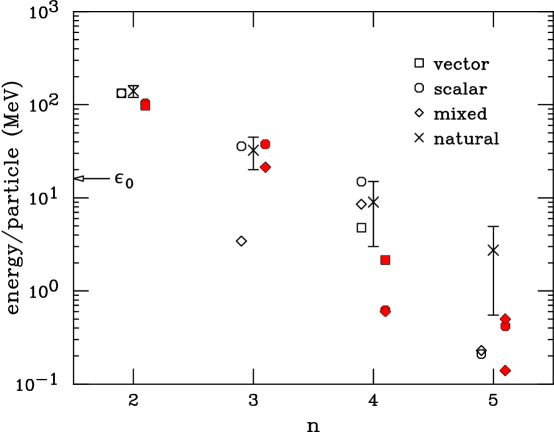
FIG. 12.: Contributions to the energy per particle in nuclear matter for parameter sets G1 and G2 from the $n^{\rm th}$-order terms of the form $\Phi^{l}W^{m}$, where $n=l+m$. The boxes are terms with $l=0$, the circles are terms with $m=0$, and absolute values are shown. Results from set G1 are open and those from G2 are filled. The crosses are estimates based on Eq. (49). The arrow indicates the total binding energy $\epsilon_{0}=16.1~{}\mbox{MeV}$.

It is instructive to examine the contributions to the energy of nuclear matter from various terms in the energy density. This is shown in Fig. 12, where the contributions to the energy per nucleon at equilibrium from the quadratic, cubic, and quartic powers of the fields $\Phi$ and $W$ in Eq. (129) are indicated separately. We set the scale for the natural size of contributions expected from an $n^{\rm th}$-order term using the power counting estimate [Eq. (49)] for an $n^{\rm th}$-order contact term and the approximation $\langle\overline{N}N\rangle\approx\langle N^{\dagger}N\rangle=\rho_{\scriptscriptstyle\rm B}$, with $\rho_{\scriptscriptstyle\rm B}$ being the baryon density and the bracket indicating an expectation value. These estimates are marked with crosses, and the error bars reflect a range of $\Lambda$ from 500 MeV to 1 GeV. We observe that the estimates are consistent with the field energies found from the fits. Furthermore, these estimates also set the scales for the mean meson fields, which are consistent with Eq. (51). This is an indication that the naturalness assumption is valid (see below).

Several observations can be made based on the figure:

• The contributions decrease steadily with increasing powers of the fields, so that a truncation is justified. Note that this decrease will become more gradual as the density is increased above equilibrium density.

• The nuclear matter binding energy (indicated by the arrow) is an order of magnitude smaller than the individual $\nu=2$ contributions. This implies that the $\nu=2$ scalar and vector contributions cancel almost completely and also that $\nu=4$ contributions are still quite significant (at least for set G1).

• The $\nu=5$ contributions [see Eq. (66)] are representative results obtained when the $\nu=4$ fit is extended. (They correspond to the lowest values of $\chi^{2}$). They are not well determined; almost identical values of $\chi^{2}$ can be found for very different $\nu=5$ parameters. Nevertheless, even when unnatural $\nu=5$ parameters are introduced, their net contribution to the energy is typically a few tenths of an MeV. Thus a truncation at $\nu=4$ is consistent and adequate.

• The systematics of the two parameter sets at $\nu=4$ are quite different. Set G1 parallels the systematics of the standard parameter sets from Refs. [73, 70, 74], while the $\nu=4$ terms for G2 are quite small. This is possible because of the contributions from the $\alpha_{1}$ and $\alpha_{2}$ terms, which involve gradients of the meson fields and thus do not contribute in nuclear matter. The contributions of these gradients [note the signs of the $\alpha_{i}$ and the signs in Eq. (64)] to the spin-orbit splittings in finite nuclei allow set G2 to accurately reproduce the empirical spectra, even though $M^{*}/M$ in nuclear matter is larger than in conventional models.

If we return now to the parameters in Table I, we see that while the Yukawa couplings and the scalar mass are close for the two sets, the meson self-couplings are very different. This is consistent with our earlier Hartree calculations [62, 13], which showed that the bulk and single-particle observables of interest are determined to a large extent by a relatively small number of nuclear properties. As noted above, by reproducing five important properties of nuclear matter and by choosing an appropriate scalar mass, one essentially fixes the predicted properties of doubly magic nuclei, and thus the thirteen parameters in the present model are underdetermined. The parameters are therefore highly correlated and are sensitive to the relative weights chosen for the observables, including the spin-orbit splittings. To determine the parameters better, one must include additional observables that are sensitive to different aspects of the dynamics.

To explore these issues further and to put our $\nu=4$ fit in perspective, it is useful to find parameter sets for more constrained truncations. If we optimize with the “standard” mean-field model, which includes the Yukawa couplings, the scalar mass, and $\kappa_{3}$ and $\kappa_{4}$, we find $\chi^{2}\approx 110$, and the parameter set (which we label Q1) is qualitatively close to the “best-fit” sets of the past and also to the corresponding parameters of set G1 (see Table I). Adding the $\nu=4$ vector self-interaction, with parameter $\zeta_{0}$, improves the $\chi^{2}$ to about 90 (set Q2). The $\chi^{2}$ values of sets G1 and G2 are slightly less than 50, so it is clear that a better fit is obtained with more parameters, but not dramatically so.

If we truncate our model at $\nu=2$ (set W1), keeping only the Yukawa couplings and the scalar mass and setting all other parameters to zero, the best $\chi^{2}$ is over 1700. The “optimal” set in this case depends strongly on the relative weights, because only a subset of the observables can be reproduced accurately. The standard choice [62] has been to reproduce the charge radii accurately at the expense of significant underbinding. The present set of weights leads to much better binding energies (despite a large compressibility) but the systematics of the charge radii (oxygen in particular) is badly reproduced. The spin-orbit splittings are too large in all cases, corresponding to a low value for $M^{*}/M$ (see Table V).

At $\nu=3$ (set C1), we add two parameters, $\kappa_{3}$ and $\eta_{1}$. (We hold $\eta_{\rho}$ at zero for simplicity.) If the number of parameters was the sole key to a good fit, we would expect $\chi^{2}$ to be comparable to that from the standard models. However, the best fit has $\chi^{2}\approx 400$. In practice the $\eta_{1}$ contribution plays the same role as $\kappa_{4}$ if one looks at energy contributions in nuclear matter, but it is insufficient to accurately reproduce nuclear sizes. It is likely that the density dependence of the two $\nu=3$ terms is too similar to provide enough flexibility for a good fit.

Thus we find that we need at least $\nu=4$ terms to find a good fit to nuclear properties. Examples are sets Q1 and Q2. Once we allow all $\nu=4$ terms, however, the fit is underdetermined, as is evident by the differences between our sets G1 and G2. One of the important new features are the $\alpha_{1}$ and $\alpha_{2}$ parameters, which accompany derivative corrections. Without these included in the fit, set G2 cannot achieve a $\chi^{2}$ better than 100.

If we include $\nu=5$ parameters from Eq. (66) in the fit, only small improvements in $\chi^{2}$ ($<2$ units) are found. The net contribution to the energy from these terms is very small (roughly a few tenths of an MeV) in these fits, even if the coefficients are artificially made large so that individual contributions are significant. Furthermore, the changes in the lower-order coefficients from the $\nu=4$ fits are small. Thus we find $\nu=4$ contributions are necessary and sufficient for this set of observables. Clearly the $\nu=5$ results, when included, do not drive the physics, and their effects can be absorbed into small changes in the lower-order couplings. The insensitivity to the $\nu=5$ terms validates our truncation of the lagrangian.

The parameters in Table I have been displayed in such a way that they should all be of order unity according to NDA and the naturalness assumption. This is seen to be the case. It is important to emphasize this nontrivial result: Without the guidance from NDA, these coefficients could be any size at all! We conclude that NDA and the naturalness assumption are indeed compatible with and implied by the observed properties of finite nuclei, even though we are absorbing many-body effects in the coefficients.

However, the detailed mechanism by which the nuclear observables constrain the parameters to be natural is not transparent. Second-order ($\nu=2$) coefficients vary only slightly, regardless of the number of parameters used. The other parameters, while natural, are not as well determined. We searched for unnatural parameter sets by starting from unnatural values, but the optimization always produced natural results. The $\nu=5$ parameters can be made large, but they are tuned by the optimization so that they cancel almost completely in the Hartree equations. Despite the narrow range of densities present in ordinary nuclei, the different density dependence of various terms in the energy is apparently sufficient to enforce naturalness.

VI Discussion and Summary

Our goals in this paper are to construct an effective field theory based on hadrons that is appropriate for calculations of finite-density nuclear systems and to propose methods for making these calculations tractable. The lagrangian is consistent with the underlying symmetries of QCD, and heavy, non-Goldstone bosons are introduced to avoid the calculation of (some) virtual pion loops. To organize the lagrangian, we rely on Naive Dimensional Analysis (NDA), which allows us to extract the dimensional scales of any term, on the assumption of naturalness, which says that the remaining dimensionless coefficient for each term should be of order unity, and on the observation that the ratios of mean meson fields (and their gradients) to the nucleon mass (which generically represents the “heavy” mass scale) are good expansion parameters. Since the meson fields are roughly proportional to the nuclear density, and since the spatial variations in nuclei are determined by the momentum distributions of the valence nucleon wave functions, this organizational scheme is essentially an expansion in $k_{\rm F}/M$, where $k_{\rm F}$ is a Fermi wavenumber corresponding to normal nuclear densities. If NDA and the naturalness assumption are valid, one can expand the lagrangian in powers of the fields and their derivatives, truncate at some finite order, and thus have some predictive power for the properties of nuclei. Our fits to bulk and single-particle nuclear properties show that this is indeed the case.

As in all effective field theories, the coefficients in our nonrenormalizable lagrangian implicitly include contributions from energy scales heavier than our generic mass $\Lambda$. Thus contributions from baryon vacuum loops and non-Goldstone boson loops (including, in principle, particles more massive than those considered here) are parametrized in this way. Moreover, since we presently compute the nuclear observables at the one-baryon-loop or Hartree level, fitting the parameters to nuclei means that they also implicitly include the effects of many-body corrections. These consist of nucleon exchange and correlation contributions, which may involve virtual states with large excitation energies, modifications of the vacuum dynamics at finite density, like the nuclear Lamb shift, and virtual pion loops, since the mean pion field vanishes in spherical nuclei. These many-body effects involve both short- and long-range dynamics, so it is notable that our fitted parameters are still natural.

We can understand this result with the following arguments. First, it is unlikely that natural parameters arise from a sensitive cancellation between unnatural parameters in the lagrangian and compensating large many-body effects. It is much more likely that the parameters in the lagrangian are natural, and the modifications from many-body effects are small. This is consistent with explicit calculations of relativistic exchange and correlation effects, which show that these contributions do not significantly modify the nucleon self-energies nor introduce large state dependence, at least for states in the Fermi sea. This “Hartree dominance” of the mean fields [13] and of the parameters needed to produce them is a crucial element in the expansion and truncation scheme described above. An important topic for future work is the explicit evaluation of correlation effects in this model, both to disentangle these contributions from the fit parameters and to verify the extent to which Hartree dominance is valid.

We can also understand why earlier relativistic Hartree approaches to nuclear structure were successful. Many of these calculations used lagrangians that were truncated arbitrarily at quartic interactions in the meson fields, but we have seen that quintic and higher-order terms are unimportant (and undetermined) for the nuclear observables of interest. Moreover, even though most of these investigations arbitrarily set some of the cubic and quartic meson parameters to zero, we have also seen that the full complement of parameters through fourth order ($\nu\leq 4$) are underdetermined by the data. Therefore, keeping only a subset of the parameters does not preclude the possibility of a realistic fit to nuclei.

In summary, we have constructed an effective lagrangian that maintains the symmetries of QCD, such as Lorentz invariance, parity conservation, chiral symmetry, and electromagnetic gauge invariance. The bulk and single-particle properties of nuclei can be described realistically by this effective hadronic theory at the one-baryon-loop level. Naive dimensional analysis and the naturalness assumption are found to be compatible with the observed nuclear properties. The fitted parameters are natural, and the results are not driven by the last terms kept. The description of the spin-orbit splittings of the least bound nucleons and the shell structure are generally good, although the errors are relatively large compared with the other observables. The long-range electromagnetic structure of the nucleon is included explicitly using vector-meson dominance and derivative couplings to the photon; it is not necessary to introduce ad hoc electromagnetic form factors. The mesonic and gradient contributions are important for reducing fluctuations in the point-nucleon charge density, and the resulting nuclear charge form factors agree well with experiment. The extension of these calculations beyond one-baryon-loop order is currently in progress.