nucl-th/9607022

Meson-Baryon-Baryon Vertex Function and the Ward-Takahashi Identity

Siwen Wang and Manoj K. Banerjee

Department of Physics, University of Maryland, College Park, MD 20742

Ohta proposed a solution for the well-known difficulty of satisfying the Ward-Takahashi identity for a photo-meson-baryon-baryon amplitude ($\gamma$MBB) when a dressed meson-baryon-baryon (MBB) vertex function is present. He obtained a form for the $\gamma$MBB amplitude which contained, in addition to the usual pole terms, longitudinal seagull terms which were determined entirely by the MBB vertex function. He arrived at his result by using a Lagrangian which yields the MBB vertex function at tree level. We show that such a Lagrangian can be neither hermitian nor charge conjugation invariant. We have been able to reproduce Ohta’s result for the $\gamma$MBB amplitude using the Ward-Takahashi identity and no other assumption, dynamical or otherwise, and the most general form for the MBB and $\gamma$MBB vertices. However, contrary to Ohta’s finding, we find that the seagull terms are not robust. The seagull terms extracted from the $\gamma$MBB vertex occur unchanged in tree graphs, such as in an exchange current amplitude. But the seagull terms which appear in a loop graph, as in the calculation of an electromagnetic form factor, are, in general, different. The whole procedure says nothing about the transverse part of the ($\gamma$MBB) vertex and its contributions to the amplitudes in question.

PACS numbers: 11.30.-j, 13.40.G, 13.60.-r

1 Introduction

In a hadronic Lagrangian based approach to baryon properties meson-baryon loops must be calculated to obtain the contribution of virtual mesons. In a wide variety of situations these loops diverge. There are two ways of dealing with the problem of divergence. One is the well-established chiral perturbation theory ($\chi$PT) [1], where only the pseudoscalar octet mesons are considered. The strategy is to use dimensional regularization and remove any divergence arising from a loop with an appropriate counterterm. The strength of the finite remainder, called a low energy constant, have to be fixed with the help of experimental data only. It may happen that one needs the physical quantity under study itself to fix the low energy constant. In such a situations $\chi$PT is unable to make a prediction.

The other popular approach is to introduce meson baryon form factors to regulate loop integrals. Unfortunately we know very little about such form factors . The practice is to extrapolate the limited information about the form factor for a range of space-like meson momentum, with the nucleon legs on mass-shell, to the full range of meson momentum using a multipole form. This very simple version of form factor may be parameterized by one or two mass parameters. The masses are guessed and are often assigned values in the range $500$ MeV to $1400$MeV. Unfortunately one has difficulty dealing with the electromagnetic properties of the baryon when one uses a phenomenological form factor in general and approximates it with an algebraically convenient form in particular. The electromagnetic vertex function $\Gamma_{\mu}^{em}(p+q,p)$, calculated at the one-loop level, as shown in Fig. 1,

Figure 1: The bare and one-loop contributions to the baryon electromagnetic vertex function. The MBB vertices are dressed.

but using form factors at the meson-nucleon vertices will not satisfy the Ward-Takahashi identity:

$$(p^{\mu}+q^{\mu}-p^{\mu})\Gamma_{\mu}^{em}(p+q,p)=p\!\!/+q\!\!/-p\!\!/-\Sigma(p+q)+\Sigma(p),$$ (1)

where $\Sigma(p)$ is the proper self-energy, $p$ and $p+q$ are the initial and final momenta. In fact, one does not even know what the expression for the self-energy is when a parameterized form factor is used without any dynamical basis.

Ohta  [2] proposes a particular path to resolving this problem. There are four features in his approach.

• He introduces an interaction Lagrangian which reproduces the meson-baryon vertex function at the tree level. Naturally the Lagrangian uses functions of the derivative operators which operates on the fields associated with the three external legs of the vertex.

• The electromagnetic interactions are generated via minimal coupling: $\partial_{\mu}\rightarrow\partial_{\mu}+iQA_{\mu}$, where $Q$ is the operator which measures the charge of the field on which $\partial_{\mu}$ operates.

• He then notes that the photo-meson amplitude resulting from his procedure contained a longitudinal seagull term expressible entirely in terms of the vertex function. The presence of this longitudinal seagull term is essential for satisfying the Ward-Takahashi identity .

• The seagull term found by Ohta is robust in the context of his theory. The same seagull term appears in any meson-baryon one loop graph where the photon interacts with an internal line . Also the seagull term appears at each meson-baryon vertex in the loop, thus generating two graphs.

Because of its simplicity Ohta’s prescription has become quite popular. Several authors have used it for one loop calculations of baryon electromagnetic and strangeness properties [3, 4, 5, 6, 7, 8].

We show that Ohta’s Lagrangian is necessarily neither hermitian nor invariant under charge conjugation. Yet we succeed in reproducing Ohta’s prescription by using only the Lorentz structure of the $\gamma$MBB vertex and the Ward-Takahashi identity itself.

Unfortunately, we also find that, in general, the resulting seagull term is not robust. It should be noted that in a tree graph with dressed vertices as in the exchange current graphs, the seagull terms are exactly those appearing in a photo-meson amplitude. A loop graph of an electromagnetic amplitude will contain a seagull term if a meson baryon form factor has been used, but, in general, it will not be the same as that appearing in a photo-meson amplitude.

The absence of robustness is established with the help of specially chosen subsets of Feynman graphs for KP$\Lambda$ and $\gamma$KP$\Lambda$ vertices. After the seagull terms in the $\gamma$KP$\Lambda$ vertex are identified, we check their robustness by considering the one loop graphs for the strangeness content of proton. As we have noted, the seagull terms act robustly in dressed tree graphs. We consider two examples. In one, the lowest order (Born) graphs are dressed only by kaon self-energy. This does generate robust seagull terms. In the other the dressing is provided by ladders of a neutral scalar meson which couples only to strangeness. The resulting seagull terms are not robust. In fact the one loop graphs for the strangeness content of proton in this case does not even have any seagull term. This example is sufficient to establish that, in general, the seagull terms identified from the $\gamma$MBB vertex are not robust.

The paper is organized as follows. The next section describes briefly Ohta’s strategy and mentions the difficulties. Section 3 discusses the lack of hermiticity and the absence of charge conjugation invariance of the Ohta Lagrangian. In section 4 we analyze general 3-point and 4-point functions related to MBB and $\gamma$MBB vertices and identify the seagull terms occurring in the latter. The result matches Ohta’s prescription. The only underlying assumption is that Lorentz and translational invariances are good symmetries of the theory. Otherwise, there is no reference to any particular dynamical model.

The robustness of the resulting seagull terms is discussed in section 5. Section 6 contains a summary of the results and conclusions.

2 The Ohta strategy and difficulty

We mentioned in the previous section that the choice of a convenient form for the form factor tells us nothing about the self-energy, thus making it impossible even to discuss the question of the Ward-Takahashi identity. One needs to know the Lagrangian which generates the form factor and the self-energy. Ohta [2] solved the problem by writing down an interaction Lagrangian which reproduces the arbitrarily guessed form factor at the tree level. Here we summarize his work very briefly. To appreciate his work fully one must read Ref. [2].

We also simplify the presentation by substituting the more realistic pseudoscalar meson field used by Ohta with a scalar field. While the substitution halves the number of independent covariant forms needed to describe the vertex function, it does not affect the thrust of this paper.

In Ohta’s approach the scalar meson-baryon-baryon form factor , $\Gamma(\ell,p)$ is reproduced at tree level by the interaction Lagrangian

$${\cal L}(x^{\prime},x,y)=\bar{\psi}(x^{\prime})\Gamma(x^{\prime},x,y)\psi(x)\phi(y).$$ (2)

It should be noted that in this approach there are no self-energy insertions on the meson and baryon lines. Hence there are no factors contributing to the vertex functions from wave function renormalizations. The quantity $\Gamma(x^{\prime},x,y)$ is the full vertex function. The Fourier transform of the nonlocal function $\Gamma(x^{\prime},x,y)$ gives the MBB vertex function $\Gamma(\ell,p)$ as follows

$$\Gamma(x^{\prime},x,y)=\int\frac{d^{4}p}{(2\pi)^{4}}\frac{d^{4}\ell}{(2\pi)^{4}}e^{i\ell\cdot(x^{\prime}-y)-ip\cdot(y-x)}\Gamma(\ell,p),$$ (3)

where $p$ and $\ell$ are the initial and final baryon momenta. One can expand the vertex function $\Gamma(\ell,p)$ in terms of a complete set of appropriate Lorentz covariant forms. A perfectly general form for a scalar meson MBB vertex is

$$\Gamma(\ell,p) = g_{0}(k^{2},\ell^{2},p^{2})+g_{1}(k^{2},\ell^{2},p^{2})(\ell\!\!/-p\!\!/)+g_{2}(k^{2},\ell^{2},p^{2})(\ell\!\!/+p\!\!/)$$ (4)

$$+ g_{3}(k^{2},\ell^{2},p^{2})[\ell\!\!/,p\!\!/],$$

$$k = p-\ell.$$ (5)

where $g_{i}(k^{2},\ell^{2},p^{2})$ are Lorentz scalar functions. Following Ohta, we introduce a generalized function of three independent momenta $\bar{\Gamma}(k,\ell,p)$ by removing the restriction imposed by Eq. (5).

$$\bar{\Gamma}(k,\ell,p) = g_{0}(k^{2},\ell^{2},p^{2})+g_{1}(k^{2},\ell^{2},p^{2})(\ell\!\!/-p\!\!/)+g_{2}(k^{2},\ell^{2},p^{2})(\ell\!\!/+p\!\!/)$$ (6)

$$+ g_{3}(k^{2},\ell^{2},p^{2})[\ell\!\!/,p\!\!/],$$

$$k \neq p-\ell,{\rm\,\,in\,\,general,}$$ (7)

and

$$\bar{\Gamma}(k=p-\ell,\ell,p)=\Gamma(\ell,p),~{}~{}~{}~{}{\rm in~{}particular}.$$ (8)

The definition of $\bar{\Gamma}(k,\ell,p)$ requires the knowledge of the analytic structure of the scalar functions $g_{i}=g_{i}(k^{2},\ell^{2},p^{2})$ which appear in Eq. (4). Note also that if we had chosen $(\ell,k)$ or $(k,p)$ as the independent pair of momenta in Eq. (4), the resulting analytically continued object $\bar{\Gamma}(k,\ell,p)$ would be different. However, Eq. (8) will continue to hold.

Ohta then introduces the electromagnetic interaction via minimal substitution. The procedure yields new seagull terms whose structure depends upon the quantities $\bar{\Gamma}(k,\ell,p)$. The explicit form of the seagull term

Figure 2: The KP$\Lambda$ vertex and Ohta’s seagull term for the photo-kaon production amplitude.

for photo-kaon production amplitude, shown in Fig. 2, is given below.

$${\cal M}^{sg}_{\mu} = -Q_{K}\frac{(2k-q)_{\mu}}{k^{2}-(k-q)^{2}}[\bar{\Gamma}(k,\ell,p)-\bar{\Gamma}(k-q,\ell,p)]$$ (9)

$$-Q_{\Lambda}\frac{(2\ell-q)_{\mu}}{\ell^{2}-(\ell-q)^{2}}[\bar{\Gamma}(k,\ell,p)-\bar{\Gamma}(k,\ell-q,p)]$$

$$-Q_{P}\frac{(p+q+p)_{\mu}}{(p+q)^{2}-p^{2}}[\bar{\Gamma}(k,\ell,p+q)-\bar{\Gamma}(k,\ell,p)]+{\cal M}^{t}_{\mu},$$

where ${\cal M}^{t}_{\mu}$ is some transverse component of ${\cal M}^{sg}_{\mu}$. Note that $k\neq p-\ell$ in the term $\bar{\Gamma}(k,\ell,p)$ which appears in Eq. (9). Note, further, that the sum of the three terms containing this factor is diveregenceless and is thus a transverse term.

Since these terms arise from a standard method of adding electromagnetic interaction to a strong interaction Lagrangian, unusual as the latter may be, it is not surprising these seagull terms, together with the usual generalized Born terms containing either a kaon pole or a baryon pole, satisfy the Ward-Takahashi identity.

Unfortunately there is a serious problem with Ohta’s prescription. The Lagrangian (2) is not hermitian if the MBB vertex $\Gamma(\ell,p)$ originally came from some Lagrangian satisfying the standard requirements of invariance under Lorentz transformation, time reversal, parity and charge conjugation. The basis of our claim is described in the next section.

3 Hermiticity and charge conjugation invariance of the Ohta Lagrangian

The baryon and kaon propagators are defined as follows. The Feynman propagators with renormalized masses are:

$$S^{0}(p) = \frac{1}{p\!\!/-M}$$

$$\Delta^{0}(k) = \frac{1}{k^{2}-m^{2}},$$ (10)

and the dressed propagators are

$$S(p) = \frac{1}{p\!\!/-M-\Sigma(p)}=\tilde{F}(p)S^{0}(p)\tilde{F}(p)$$

$$\Delta(k) = \frac{1}{k^{2}-m^{2}-\Sigma(k)}=\tilde{f}(k^{2})\Delta^{0}(k)\tilde{f}(k^{2}),$$ (11)

where the functions $\tilde{F}(p)=A(p^{2})+p\!\!/B(p^{2})$ and $\tilde{f}(k^{2})$ are introduced to incorporate the contribution of wave function renormalizations to the general vertex function. $A(p^{2})$, $B(p^{2})$ and $\tilde{f}(k^{2})$ can be expressed in terms of the baryon and meson self-energies.

Next we introduce the three-point functions, $G(\ell,p)$ and $G^{\prime}(p,\ell)$ and the vertex functions, $\Gamma(\ell,p)$ and $\Gamma^{\prime}(p,\ell)$ corresponding to the graphs as shown in Fig. 3.

(a)                                                  (b)

Figure 3: (a) corresponds to proton becoming $\Lambda$ and $K^{+}$. The associated vertex function is $\Gamma(\ell,p)$. (b) correspond to $\Lambda$ becoming proton and $K^{-}$. The associated vertex function is $\Gamma^{\prime}(p,\ell)$.

$$G(\ell,p) = \int d^{4}xe^{i\ell\cdot x}\int d^{4}ye^{-ip\cdot y}\langle 0\mid T(\psi^{\Lambda}(x)\phi(0)\bar{\psi}^{P}(y))\mid 0\rangle$$ (12)

$$= -i\tilde{F}_{\Lambda}(\ell)S^{0}_{\Lambda}(\ell)\Gamma(\ell,p)S^{0}_{P}(p)\tilde{F}_{P}(p)\Delta^{0}(p-\ell)\tilde{f}((p-\ell)^{2}),$$

$$G^{\prime}(p,\ell) = \int d^{4}xe^{-i\ell\cdot x}\int d^{4}ye^{ip\cdot y}\langle 0\mid T(\psi^{P}(y)\phi^{*}(0)\bar{\psi^{\Lambda}}(x))\mid 0\rangle$$ (13)

$$= -i\tilde{F}_{P}(p)S^{0}_{P}(p)\Gamma^{\prime}(p,\ell)S^{0}_{\Lambda}(\ell)\tilde{F}_{\Lambda}(\ell)\Delta^{0}(\ell-p)\tilde{f}((p-\ell)^{2}).$$

We take it that the vertex functions have been generated by a Lagrangian which is invariant under charge conjugation. Naturally, the resulting vacuum is even under charge conjugation. Exploiting this fact we find that

$$G_{\alpha,\beta}(\ell,p) = \int d^{4}xe^{i\ell\cdot x}\int d^{4}ye^{-ip\cdot y}\langle{\cal C}0\mid T(\psi^{\Lambda}_{\alpha}(x)\phi(0)\bar{\psi}^{P}_{\beta}(y))\mid{\cal C}0\rangle$$ (14)

$$= \int d^{4}xe^{i\ell\cdot x}\int d^{4}ye^{-ip\cdot y}\langle 0\mid{\cal C}T(\psi^{\Lambda}_{\alpha}(x)\phi(0)\bar{\psi}^{P}_{\beta}(y)){\cal C}^{-1}\mid 0\rangle$$

$$= \int d^{4}xe^{i\ell\cdot x}\int d^{4}ye^{-ip\cdot y}C_{\alpha\alpha^{\prime}}\langle 0\mid T(\psi^{P}_{\beta^{\prime}}(y)\phi^{*}(0)\bar{\psi}^{\Lambda}_{\alpha^{\prime}}(x))\mid 0\rangle C^{-1}_{\beta^{\prime}\beta},$$

where the matrix $C$ is given by

$$C=i\gamma^{2}\gamma^{0}=-C^{-1}.$$ (15)

By using the definition of $G^{\prime}(p,\ell)$, given by Eq. (13) we obtain

$$G_{\alpha,\beta}(\ell,p) = \int d^{4}xe^{i\ell\cdot x}\int d^{4}ye^{-ip\cdot y}C_{\alpha\alpha^{\prime}}\langle 0\mid T(\psi^{P}_{\beta^{\prime}}(y)\phi^{*}(0)\bar{\psi}^{\Lambda}_{\alpha^{\prime}}(x))\mid 0\rangle C^{-1}_{\beta^{\prime}\beta}$$ (16)

$$= C_{\alpha\alpha^{\prime}}G^{\prime}_{\beta^{\prime},\alpha^{\prime}}(-p,-\ell)C^{-1}_{\beta^{\prime}\beta}$$

$$= (CG^{\prime\rm T}(-p,-\ell)C^{-1})_{\alpha\beta},$$

that is,

$$G(\ell,p)=CG^{\prime\rm T}(-p,-\ell)C^{-1},$$ (18)

where the superscript T is for the transpose. The fact that $Cp\!\!/^{T}C^{-1}=-p\!\!/$ leads to results

$$CS^{0}(-p)^{T}C^{-1}=S^{0}(p)\,\,\,\,{\rm and}\,\,\,\,C\tilde{F}(-p)^{T}C^{-1}=\tilde{F}(p).$$ (19)

Using the above equation and Eqs.(18) and (13) we have

$$\Gamma(\ell,p)=C\Gamma^{\prime\rm T}(-p,-\ell)C^{-1}.$$ (20)

We recall the expansion of $\Gamma(\ell,p)$, given by Eq. (4) and supplement it with the corresponding expansion of $\Gamma^{\prime}(p,\ell)$:

$$\Gamma(\ell,p) = g_{0}(k^{2},\ell^{2},p^{2})+g_{1}(k^{2},\ell^{2},p^{2})(\ell\!\!/-p\!\!/)+g_{2}(k^{2},\ell^{2},p^{2})(\ell\!\!/+p\!\!/)$$

$$+ g_{3}(k^{2},\ell^{2},p^{2})[\ell\!\!/,p\!\!/],$$

$$\Gamma^{\prime}(p,\ell) = g^{\prime}_{0}(k^{2},p^{2},\ell^{2})+g^{\prime}_{1}(k^{2},p^{2},\ell^{2})(p\!\!/-\ell\!\!/)+g^{\prime}_{2}(k^{2},p^{2},\ell^{2})(p\!\!/+\ell\!\!/)$$ (21)

$$+ g^{\prime}_{3}(k^{2},p^{2},\ell^{2})[p\!\!/,\ell\!\!/].$$

Combining Eq. (20) with these expansions we find the following symmetry relations between the two sets of Lorentz scalar functions $g_{i}$ and $g^{\prime}_{i}$

$$g_{0}(k^{2},\ell^{2},p^{2}) = g^{\prime}_{0}(k^{2},p^{2},\ell^{2}),$$

$$g_{1}(k^{2},\ell^{2},p^{2}) = -g^{\prime}_{1}(k^{2},p^{2},\ell^{2}),$$

$$g_{2}(k^{2},\ell^{2},p^{2}) = g^{\prime}_{2}(k^{2},p^{2},\ell^{2}),$$

$$g_{3}(k^{2},\ell^{2},p^{2}) = g^{\prime}_{3}(k^{2},p^{2},\ell^{2}),$$ (22)

The Ohta Lagrangian which generates the two vertex functions of Fig. (3) at the tree level is the following:

$${\cal L}_{int} = \int\frac{d^{4}p}{(2\pi)^{4}}\int\frac{d^{4}\ell}{(2\pi)^{4}}e^{i\ell\cdot x-ip\cdot y+i(p-\ell)\cdot z}\bar{\psi}^{\Lambda}(x)\Gamma(\ell,p)\phi(z)\psi^{P}(y)$$ (23)

$$+ \int\frac{d^{4}p}{(2\pi)^{4}}\int\frac{d^{4}\ell}{(2\pi)^{4}}e^{-i\ell\cdot x+ip\cdot y-i(p-\ell)\cdot z}\bar{\psi}^{P}(y)\Gamma^{\prime}(p,\ell)\phi^{*}(z)\psi^{\Lambda}(x).$$

The requirement that ${\cal L}_{int}$ be hermitian demands that

$$\Gamma^{\prime}(p,\ell)=\gamma_{0}\Gamma^{\dagger}(\ell,p)\gamma_{0}.$$ (24)

Using the above equation in conjunction with the expansions given in Eq. (21) and the relations of Eq. (22) we find that the hermiticity of the Ohta’s Lagrangian demands that

$$g_{i}(k^{2},\ell^{2},p^{2})=g_{i}^{*}(k^{2},\ell^{2},p^{2}).$$ (25)

In other words, hermiticity of the interaction Lagrangian combined with charge-conjugation invariance of the fundamental dynamics demands that the coefficient functions be always real. However, it is well known that they are necessarily complex when $\ell^{2}$, $p^{2}$ and $(p-\ell)^{2}$ have appropriate values. Thus for example, when $\ell^{2}=M_{\Lambda}^{2}$, $p^{2}=M_{P}^{2}$ and $(p-\ell)^{2}\geq 9m^{2}$ the functions $g_{i}$ will become complex. In a realistic situation with pions present the analytic structure is richer with threshold occurring at lower masses. The reader may also verify the essential points of the preceding remarks by studying the vertex function at one-loop level of any form.

4 The Ward-Takahashi identity and $\gamma$MBB vertex

In this section we reproduce Ohta’s final result for $\gamma$MBB vertex using solely the Ward-Takahashi identity and the freedom to add divergenceless, i.e., transverse, parts to the expressions. No reference is made to any particular Lagrangian or dynamical model.

At the center is the four-point function $\langle T(\psi^{\Lambda}(x^{\prime})\bar{\psi}^{P}(x)\phi(y)J_{\mu}(z))\rangle$, where $J_{\mu}(z)$ is the electromagnetic current. The fields satisfy the equal time commutation relations:

$$\delta(x_{0}-y_{0})[J_{0}(x),\psi(y)] = -\delta^{4}(x-y)Q_{\psi}\psi(x),$$

$$\delta(x_{0}-y_{0})[J_{0}(x),\phi(y)] = -\delta^{4}(x-y)Q_{\phi}\phi(x),$$ (26)

where $Q_{\psi}$ and $Q_{\phi}$ are the charges of the particles described by the fields. Using these equal time commutation relations one obtains the following expression for the divergence of the four-point function:

$$\partial^{\mu}_{z}\langle T(\psi^{\Lambda}(x^{\prime})\bar{\psi}^{P}(x)\phi(y)J_{\mu}(z))\rangle = -[Q_{\Lambda}\delta^{4}(x^{\prime}-z)-Q_{P}\delta^{4}(x-z)+Q_{K}\delta^{4}(y-z)]$$ (27)

$$\times\langle T(\psi^{\Lambda}(x^{\prime})\bar{\psi}^{P}(x)\phi(y))\rangle$$

The $\gamma$MBB vertex function, represented by the first graph in Fig. 4 is defined by the equation

$$i\int d^{4}xe^{i\ell\cdot x}\int d^{4}x^{\prime}e^{-ip\cdot x^{\prime}}\int d^{4}ye^{ik\cdot y}\langle T(\psi^{\Lambda}(x^{\prime})\bar{\psi}^{P}(x)\phi(y)J_{\mu}(0))\rangle$$ (28)

$$= \tilde{F}_{\Lambda}(\ell)S^{0}_{\Lambda}(\ell)\tilde{f}(k^{2})\Delta^{0}(k){\cal M}_{\mu}(k,\ell,p)S^{0}_{P}(p)\tilde{F}_{P}(p),$$

Using Eqs. (12), (27) and (28) and after amputating the external factor $\tilde{F}_{\Lambda}(\ell)S^{0}_{\Lambda}(\ell)$, $S^{0}_{P}(p)\tilde{F}_{P}(p)$ and $\Delta^{0}(k)\tilde{f}(k^{2})$, we obtain the Ward-Takahashi identity:

$$q^{\mu}\cdot{\cal M}_{\mu} = Q_{K}\Delta^{0}(k)^{-1}\tilde{f}^{-1}(k^{2})\Delta^{0}(k-q)\tilde{f}((k-q)^{2})\Gamma(\ell,p)$$ (29)

$$- Q_{P}\Gamma(\ell,p+q)S^{0}_{P}(p+q)\tilde{F}_{P}(p+q)\tilde{F}^{-1}_{P}(p)S^{0}_{P}(p)^{-1}$$

$$+ Q_{\Lambda}S^{0}_{\Lambda}(\ell)^{-1}\tilde{F}^{-1}_{\Lambda}(\ell)\tilde{F}_{\Lambda}(\ell-q)S^{0}_{\Lambda}(\ell-q)\Gamma(\ell-q,p).$$

Following the standard practice, we express ${\cal M}_{\mu}$ as a sum of three ‘pole’ terms, defined by us, and the remainder, which is free of meson or baryon poles. This is exhibited in Fig. 4. Thus by definition the last term is the seagull term. A further refinement of the definition of the ‘seagull’ term will follow. The ‘pole’ terms are not pure poles as they contain the full MBB vertex function. A pure pole term will have the appropriate momentum in the vertex function on its mass shell. The electromagnetic vertices in the pole terms are just the lowest order terms with renormalized charges. Thus the photo-kaon vertex is $-iQ_{K}\Gamma^{(K)em}_{\mu}(k,k-q)=-iQ_{K}(2k-q)_{\mu}$.

Figure 4: The $\gamma$MBB vertex ${\cal M}_{\mu}(k,\ell,p)=$ three pole terms + a seagull part

The expression for ${\cal M}^{pole}_{\mu}$, the sum of the three pole terms of Fig. 4 with the renormalized charges, is

$${\cal M}^{pole}_{\mu} = Q_{K}\Gamma_{\mu}^{(K)em}(k,k-q)\Delta^{0}(k-q)\Gamma(\ell,p)$$ (30)

$$+ Q_{\Lambda}\Gamma_{\mu}^{(\Lambda)em}(\ell,\ell-q)S^{0}_{\Lambda}(\ell-q)\Gamma(\ell-q,p)$$

$$+ Q_{P}\Gamma(\ell,p+q)S^{0}_{P}(p+q)\Gamma_{\mu}^{(P)em}(p+q,p),$$

The Ward-Takahashi identities for these vertices are,

$$q^{\mu}\cdot\Gamma_{\mu}^{(K)em}(k,k-q) = \Delta^{0}(k)^{-1}-\Delta^{0}(k-q)^{-1}$$

$$q^{\mu}\cdot\Gamma_{\mu}^{(\Lambda)em}(\ell,\ell-q) = S^{0}_{\Lambda}(\ell)^{-1}-S^{0}_{\Lambda}(\ell-q)^{-1}$$

$$q^{\mu}\cdot\Gamma_{\mu}^{(P)em}(p+q,p) = S^{0}_{P}(p+q)^{-1}-S^{0}_{P}(p)^{-1}$$ (31)

The divergence of the ${\cal M}^{pole}_{\mu}$ is

$$q^{\mu}\cdot{\cal M}^{pole}_{\mu} = Q_{K}[\Delta^{0}(k)^{-1}\Delta^{0}(k-q)-1]\Gamma(l,p)$$ (32)

$$+ Q_{P}\Gamma(\ell,p+q)[1-S^{0}_{P}(p+q)S^{0}_{P}(p)^{-1}]$$

$$+ Q_{\Lambda}[S^{0}_{\Lambda}(\ell)^{-1}S^{0}_{\Lambda}(\ell-q)-1]\Gamma(\ell-q,p)$$

By definition

$${\cal M}^{sg}_{\mu}={\cal M}_{\mu}-{\cal M}^{pole}_{\mu}$$ (33)

From Eqs. (29) and (32) we have

$$q^{\mu}\cdot{\cal M}^{sg}_{\mu} = q^{\mu}\cdot({\cal M}_{\mu}-{\cal M}^{pole}_{\mu})$$ (34)

$$= Q_{K}\Gamma(\ell,p)[1-\Delta^{0}(k)^{-1}\tilde{f}^{-1}(k^{2})\Delta^{0}(k-q)(\tilde{f}(k^{2})-\tilde{f}((k-q)^{2}))]$$

$$+ Q_{\Lambda}[1-S^{0}_{\Lambda}(\ell)^{-1}\tilde{F}^{-1}_{\Lambda}(\ell)(\tilde{F}_{\Lambda}(\ell)-\tilde{F}_{\Lambda}(\ell-q))S^{0}_{\Lambda}(\ell-q)]\Gamma(\ell-q,p)$$

$$- Q_{P}\Gamma(\ell,p+q)[1-S^{0}_{P}(p+q)(\tilde{F}_{P}(p)-\tilde{F}_{P}(p+q))\tilde{F}^{-1}_{P}(p)S^{0}_{P}(p)^{-1}].$$

The vertex functions in Eq. (34) all satisfy momentum conservation. For future convenience in matching our result with that of Ohta we write these as $\bar{\Gamma}(k-q,\ell,p)$, etc. using Eq. (8). The longitudinal part of ${\cal M}^{sg}_{\mu}$ is fixed by the Ward-Takahashi identity and we may write the solution of Eq. (34) in the form:

$${\cal M}^{sg}_{\mu} = Q_{K}\frac{(2k-q)_{\mu}}{k^{2}-(k-q)^{2}}\bar{\Gamma}(k-q,\ell,p)[1-\Delta^{0}(k)^{-1}\tilde{f}^{-1}(k^{2})\Delta^{0}(k-q)(\tilde{f}(k^{2})-\tilde{f}((k-q)^{2}))]$$ (35)

$$+ Q_{\Lambda}\frac{(2\ell-q)_{\mu}}{\ell^{2}-(\ell-q)^{2}}[1-S^{0}_{\Lambda}(\ell)^{-1}\tilde{F}^{-1}_{\Lambda}(\ell)(\tilde{F}_{\Lambda}(\ell)-\tilde{F}_{\Lambda}(\ell-q))S^{0}_{\Lambda}(\ell-q)]\Gamma(\ell-q,p)$$

$$- Q_{P}\frac{(p+q+p)_{\mu}}{(p+q)^{2}-p^{2}}\bar{\Gamma}(k,\ell,p+q)[1-S^{0}_{P}(p+q)(\tilde{F}_{P}(p)-\tilde{F}_{P}(p+q))\tilde{F}^{-1}_{P}(p)S^{0}_{P}(p)^{-1}]$$

$$+ {\cal M}^{t}_{\mu},$$

where ${\cal M}^{t}_{\mu}$ is an unknown transverse part. The preceding expression contains many pieces involving propagators and wave function renormalization factors which do not appear in Ohta’s treatment. The reason is that the latter is based on a very special dynamics while the result here is completely general. However, we note that these extra terms all vanish when the external legs are on their respective mass shells, i.e., $k^{2}=m^{2}$ and one replaces $p\!\!/$ with $M_{P}$ and $\ell\!\!/$ with $M_{\Lambda}$. Exploiting this we propose that the general result should be compared with Ohta’s on the mass shell only. Whereupon we have

$${\cal M}^{sg}_{\mu} = Q_{K}\frac{(2k-q)_{\mu}}{k^{2}-(k-q)^{2}}\bar{\Gamma}(k-q,\ell,p)+Q_{\Lambda}\frac{(2\ell-q)_{\mu}}{\ell^{2}-(\ell-q)^{2}}\bar{\Gamma}(k,\ell-q,p)$$ (36)

$$-Q_{P}\frac{(p+q+p)_{\mu}}{(p+q)^{2}-p^{2}}\bar{\Gamma}(k,\ell,p+q)+{\cal M}^{t}_{\mu}.$$

The solution still does not quite match Ohta’s result. It also has the unpleasant feature that it is singular when either $q\rightarrow 0$ or $k^{2}\rightarrow(k-q)^{2}$ etc. We rectify the problem by choosing following form for ${\cal M}^{t}_{\mu}$:

$${\cal M}^{t}_{\mu}={\cal M}^{t}_{1,\mu}+{\cal M}^{t}_{2,\mu}+{\cal M}^{t}_{3,\mu},$$ (37)

where

$${\cal M}^{t}_{1,\mu} = -Q_{K}\frac{(2k-q)_{\mu}}{k^{2}-(k-q)^{2}}\bar{\Gamma}(k,\ell,p)-Q_{\Lambda}\frac{(2\ell-q)_{\mu}}{\ell^{2}-(\ell-q)^{2}}\bar{\Gamma}(k,\ell,p)$$ (38)

$$+Q_{P}\frac{(p+q+p)_{\mu}}{(p+q)^{2}-p^{2}}\bar{\Gamma}(k,\ell,p),$$

which ensures the finiteness of ${\cal M}^{sg}_{\mu}$ as $q\rightarrow 0$ or $k^{2}=(k-q)^{2}$, and

$${\cal M}^{t}_{2,\mu} = Q_{\Lambda}\{\frac{(2\ell-q)_{\mu}}{\ell^{2}-(\ell-q)^{2}}q\!\!\!/-\gamma_{\mu}\}[g_{1}(k^{2},(\ell-q)^{2},p^{2})+g_{2}(k^{2},(\ell-q)^{2},p^{2})]$$ (39)

$$+Q_{\Lambda}\{\frac{(2\ell-q)_{\mu}}{\ell^{2}-(\ell-q)^{2}}[q\!\!\!/,p\!\!\!/]+2i\sigma_{\mu\nu}p^{\nu}\}g_{3}(k^{2},(\ell-q)^{2},p^{2})$$

$$+Q_{P}\{\frac{(p+p+q)_{\mu}}{(p+q)^{2}-p^{2}}q\!\!\!/-\gamma_{\mu}\}[g_{1}(k^{2},\ell^{2},(p+q)^{2})+g_{2}(k^{2},\ell^{2},(p+q)^{2})]$$

$$+Q_{P}\{\frac{(p+p+q)_{\mu}}{(p+q)^{2}-p^{2}}[\ell\!\!\!/,q\!\!\!/]+2i\sigma_{\nu\mu}\ell^{\nu}\}g_{3}(k^{2},\ell^{2},(p+q)^{2}),$$

which guarantees the regularities of ${\cal M}^{sg}_{\mu}$ when either $\ell^{2}=(\ell-q)^{2}$ or $(p+q)^{2}=p^{2}$. The quantity ${\cal M}^{t}_{3,\mu}$ is still some undetermined transverse term which is however free from unphysical singularities.

Keep in mind that while $\bar{\Gamma}(k-q,\ell,p)=\Gamma(\ell,p)$, $\bar{\Gamma}(k,\ell-q,p)=\Gamma(\ell-q,p)$ and $\bar{\Gamma}(k,\ell,p+q)=\Gamma(\ell,p+q)$ are true vertex functions satisfying the momentum conservation, $\bar{\Gamma}(k,\ell,p)$, which is defined via analytical continuation of $g_{i}$ etc in Eqs. (6) and (7), is equal to a physical MBB vertex at $q=0$ only.

Eqs. (36), (38) and (39) together give us the following result for the seagull vertex

$${\cal M}^{sg}_{\mu} = -Q_{K}\frac{(2k-q)_{\mu}}{k^{2}-(k-q)^{2}}[\bar{\Gamma}(k,\ell,p)-\bar{\Gamma}(k-q,\ell,p)]$$ (40)

$$-Q_{\Lambda}\frac{(2\ell-q)_{\mu}}{\ell^{2}-(\ell-q)^{2}}[\bar{\Gamma}(k,\ell,p)-\bar{\Gamma}(k,\ell-q,p)]$$

$$-Q_{P}\frac{(p+q+p)_{\mu}}{(p+q)^{2}-p^{2}}[\bar{\Gamma}(k,\ell,p+q)-\bar{\Gamma}(k,\ell,p)]$$

$$+Q_{\Lambda}\{\frac{(2\ell-q)_{\mu}}{\ell^{2}-(\ell-q)^{2}}q\!\!\!/-\gamma_{\mu}\}[g_{1}(k^{2},(\ell-q)^{2},p^{2})+g_{2}(k^{2},(\ell-q)^{2},p^{2})]$$

$$+Q_{\Lambda}\{\frac{(2\ell-q)_{\mu}}{\ell^{2}-(\ell-q)^{2}}[q\!\!\!/,p\!\!\!/]+2i\sigma_{\mu\nu}p^{\nu}\}g_{3}(k^{2},(\ell-q)^{2},p^{2})$$

$$+Q_{P}\{\frac{(p+p+q)_{\mu}}{(p+q)^{2}-p^{2}}q\!\!\!/-\gamma_{\mu}\}[g_{1}(k^{2},\ell^{2},(p+q)^{2})+g_{2}(k^{2},\ell^{2},(p+q)^{2})]$$

$$+Q_{P}\{\frac{(p+p+q)_{\mu}}{(p+q)^{2}-p^{2}}[\ell\!\!\!/,q\!\!\!/]+2i\sigma_{\nu\mu}\ell^{\nu}\}g_{3}(k^{2},\ell^{2},(p+q)^{2}).$$

$$+{\cal M}^{t}_{3,\mu}.$$

We find that Eq. (40) would be exactly equal to Ohta’s result had he discussed the case of a scalar meson instead of a pseudoscalar meson and chosen to expand the vertex function $\Gamma(\ell,p)$ in the form of Eq. (21) of this paper instead of Eq.(2.12) of Ref. [2].

Since Ohta introduced a very special dynamics, namely, an interaction Lagrangian which generates the complete vertex function at the tree level, he had another remarkable results. His seagull term, obtained initially from an analysis of the $\gamma$MBB amplitude, is robust and appears in all electromagnetic processes which involve one or more MBB vertex calculated with his Lagrangian. While we duplicate his result for the $\gamma$MBB amplitude, the seagull term obtained by us will not appear in unmodified form in graphs involving charged meson loops. However, a tree graph, such as an exchange current amplitude, will have the same seagull term without modification. We explain the claim in the next section.

5 Robustness of the Seagull Term

Robustness of the seagull terms is best examined in terms of subsets of diagrams generated from a field theory satisfying the standard requirements of invariances and symmetries.

The essence of this approach is to take a Lagrangian and choose suitable but consistent subsets of diagrams for the various physical quantities like the self-energy , the meson-baryon vertex function, and the electromagnetic amplitudes, etc and demonstrate that the seagull terms, obtained from an analysis of the $\gamma$MBB vertex cannot be used in toto when charged meson loops are present. In principle, one example is sufficient. It is also sufficient in practical terms if the example contains graphs which are manifestly important.

Since we select diagrams we need not spell out the Lagrangian as long as there exists a Lagrangian which generates the diagrams we are considering. To reduce the number of types of diagrams we need to consider we confine ourselves to those which contribute to the strangeness content of the proton. Operationally, this means that our photon couples to strangeness and not to charge. Therefore for the discussion of this section we have

$$Q_{P}=0,\,\,\,\,Q_{K}=-Q_{\Lambda}.$$ (41)

Having chosen a subset of graphs we do the following: First we define our MBB vertex function by choosing a subset of Feynman diagrams for it. Then we couple a photon to an internal kaon or $\Lambda$ in all possible ways and sum them up to obtain the resulting $\gamma$MBB vertex function. The procedure is guaranteed to yield vertex function which satisfies the Ward-Takahashi identity in terms of the MBB vertex function, already defined. The full electromagnetic vertex function is easily divide into two subsets - one containing the pole terms, defined in section 4, the other constitute the seagull terms ${\cal M}^{sg}_{\mu}$.

We test the robustness of the seagull terms obtained from the $\gamma$MBB vertex by constructing the kaon-$\Lambda$ loop which appear in the $\gamma$BB electromagnetic amplitude and examining the seagull terms appearing in it to check if they are the same as the ones from the $\gamma$MBB vertex. It is straightforward to see that the seagull terms will act in a robust manner in exchange current graphs, i.e., tree graphs with dressed vertices.

We consider two contrasting examples. In the first example the the KP$\Lambda$ and the $\gamma$KP$\Lambda$ vertices arise entirely from the proper self energy of the kaon. The baryon propagators are bare propagators with renormalized masses. In this case we find that the seagull terms of the $\gamma$KP$\Lambda$ vertex are robust. They appear unmodified in the kaon-$\Lambda$ loop term of the $\gamma$BB electromagnetic amplitude . The one loop diagrams for nucleon self-energy are also structurally similar to those of Ohta. Dressed KP$\Lambda$ vertices appear at both ends of the loop.

In the second example, the KP$\Lambda$ vertex is dressed by a ladder of scalar meson exchanges between the internal kaon and $\Lambda$ hyperon. Here we find that while the $\gamma$KP$\Lambda$ has the usual Ohta type seagull terms, the kaon-$\Lambda$ loop which appear in the $\gamma$BB electromagnetic amplitude does not even have a seagull term. We also note that the one loop diagrams for nucleon self-energy are also structurally different from those of Ohta. The dressed KP$\Lambda$ vertex appears at only one end of the loop.

5.1 Kaon self-energy and the KP$\Lambda$ vertex

We begin with an examination of the fully dressed kaon propagator, $\Delta(k^{2})$, which appears in the KP$\Lambda$ vertex shown in Fig. 5.

Figure 5: The KP$\Lambda$ vertex with dressed kaon propagator, but bare KP$\Lambda$ coupling. The circle represents kaon self-energy, not the proper self-energy, $\Sigma(k^{2})$.

We write

$$\Delta(k^{2})=\frac{1}{k^{2}-m^{2}-\Sigma(k^{2})},$$ (42)

where, by definition, $\Sigma(m^{2})=0$, $m$ being the renormalized kaon mass. This allows us to write $\Sigma(k^{2})=(k^{2}-m^{2})\bar{\Sigma}(k^{2})$, where $\bar{\Sigma}(k^{2})$ is analytic in the neighborhood of $k^{2}=m^{2}$. Finally, we write

$$\Delta(k^{2})=\frac{[\tilde{f}(k^{2})]^{2}}{k^{2}-m^{2}},$$ (43)

where $\tilde{f}(k^{2})=[1-\bar{\Sigma}(k^{2})]^{-1/2}$ is the wave function renormalization factor in the present case. With $g^{0}_{KN\Lambda}$ as the bare coupling constant, the renormalized coupling constant is

$$g_{KN\Lambda}=g^{0}_{KN\Lambda}\tilde{f}(m^{2}).$$ (44)

Amputating the baryon legs, the expression for the amplitude, shown in Fig. 5, is

$${\cal A}(p-k,k)=g_{KN\Lambda}f(k^{2})\frac{\tilde{f}(k^{2})}{k^{2}-m^{2}},$$ (45)

where

$$f(k^{2})=\frac{\tilde{f}(k^{2})}{\tilde{f}(m^{2})},$$ (46)

is the KP$\Lambda$ form factor, normalized to $f(m^{2})=1$. The last factor in Eq. (45) is removed during amputation of the external propagator.

Figure 6: The photo-kaon amplitude. For brevity, graphs where the photon couples to the $\Lambda$ have been omitted. The baryon propagators have been amputated.

The photo-kaon amplitude, in the present context, is exhibited in Fig 6. For brevity, all graphs where the photon couples to the $\Lambda$ have been omitted.The point we wish to make can be made without any reference to the omitted graphs. The expression for the abbreviated amplitude is given by

$${\cal M}^{\prime}_{\mu}=Q_{K}g^{0}_{KN\Lambda}\Delta(k^{2})\bar{\Gamma}^{(K)em}_{\mu}(k,k^{\prime})\Delta(k^{\prime 2}),$$ (47)

where $\bar{\Gamma}^{(K)em}_{\mu}(k,k^{\prime})$ is the kaon electromagnetic vertex and

$$k^{\prime}=k-q.$$ (48)

Note that the kaon electromagnetic vertex function $\bar{\Gamma}^{(K)em}_{\mu}(k,k^{\prime})$ here is different from the $\Gamma^{(K)em}_{\mu}(k,k^{\prime})$ as defined in Eq. (30) in that it satisfies the Ward-Takahashi identity in connection with the fully dressed kaon propagators

$$q^{\mu}\bar{\Gamma}^{(K)em}_{\mu}(k,k^{\prime})=\Delta(k^{2})^{-1}-\Delta(k^{\prime 2})^{-1}.$$ (49)

Following our practice we drop the transverse part of $\bar{\Gamma}^{(K)em}_{\mu}(k,k^{\prime})$ and choose for the remainder, the longitudinal part, the form [9]:

$$\bar{\Gamma}^{(K)em}_{\mu}(k,k^{\prime})=(k^{\prime}+k)_{\mu}\frac{\Delta(k^{\prime 2})^{-1}-\Delta(k^{2})^{-1}}{k^{\prime 2}-k^{2}}.$$ (50)

Adding and subtracting the first term on the right hand side of the equation below to the expression for ${\cal M}^{\prime}_{\mu}$, given by Eq. (47), and using Eq. (43) we obtain

$${\cal M}^{\prime}_{\mu}=Q_{K}g^{0}_{KN\Lambda}(k^{\prime}+k)_{\mu}[\frac{\tilde{f}(k^{\prime 2})\tilde{f}(k^{2})}{(k^{\prime 2}-m^{2})(k^{2}-m^{2})}$$

$$-\frac{\tilde{f}(k^{\prime 2})-\tilde{f}(k^{2})}{k^{\prime 2}-k^{2}}\frac{\tilde{f}(k^{2})}{k^{2}-m^{2}}-\frac{\tilde{f}(k^{\prime 2})-\tilde{f}(k^{2})}{k^{\prime 2}-k^{2}}\frac{\tilde{f}(k^{\prime 2})}{k^{\prime 2}-m^{2}}]$$ (51)

Next, we amputate the external kaon leg. This requires dividing the expression in Eq. (51 ) by the factor $\tilde{f}(k^{2})/(k^{2}-m^{2})$, obtaining

$${\cal M}^{\prime\prime}_{\mu}=Q_{K}g^{0}_{KN\Lambda}(k^{\prime}+k)_{\mu}[\frac{\tilde{f}(k^{\prime 2})}{k^{\prime 2}-m^{2}}$$

$$-\frac{\tilde{f}(k^{\prime 2})-\tilde{f}(k^{2})}{k^{\prime 2}-k^{2}}-\frac{\tilde{f}(k^{\prime 2})-\tilde{f}(k^{2})}{k^{\prime 2}-k^{2}}\frac{\tilde{f}(k^{\prime 2})}{k^{\prime 2}-m^{2}}\frac{k^{2}-m^{2}}{\tilde{f(k^{2})}}]$$ (52)

One may verify that the second and third terms in above expression for ${\cal M}^{\prime\prime}_{\mu}$ agree with the terms multiplying $Q_{K}$ in Eqs. (35) and (38) of section 4 provided we set the KP$\Lambda$ vertex $\bar{\Gamma}(k-q,\ell,p)=g^{0}_{KN\Lambda}\tilde{f}(k^{\prime 2})$. We also note that if we had included here graphs where the photon couples to $\Lambda$ and had also included $\Lambda$ self-energy insertions we would have a result which matched the terms multiplying $Q_{\Lambda}$.

Finally we let $k^{2}\rightarrow m^{2}$ and the last term of Eq. (52) drops out. Upon using Eqs (44) and (46) the amputated amplitude becomes

$${\cal M}_{\mu}=Q_{K}g_{KN\Lambda}(k^{\prime}+k)_{\mu}[\frac{f(k^{\prime 2})}{k^{\prime 2}-m^{2}}-\frac{f(k^{2})-f(k^{\prime 2})}{k^{2}-k^{\prime 2}}].$$ (53)

The first term is the traditional generalized Born graph with dressed KP$\Lambda$ vertex and the second term is the , by now, familiar seagull term of the Ohta form.

We end this subsection by noting that

• (a) because of the simplicity of the dynamics the amplitude does not depend upon baryon momentum squares,

• (b) and that the expression in Eq. (51) is fully symmetric in $k$ and $k^{\prime}$.

5.2 Special dressing of the KP$\Lambda$ vertex

We consider the set of graphs which dresses the KP$\Lambda$ vertex with a complete set of ladders of scalar meson exchanges between the internal kaon and $\Lambda$ hyperon. By our definition, the scalar meson couples to strangeness only. We call it the $\sigma$ meson and use (gluon-like) helices for its propagators in a Feynman graph. The complete set of ladders of $\sigma$ exchange, constituting a K-$\Lambda$ scattering amplitude, is shown in Fig. 7.

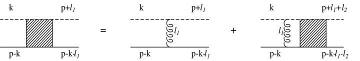
Figure 7: The K-$\Lambda$ scattering amplitude.

In Fig. 8 we show the dressing of the KP$\Lambda$ vertex with a complete set of $\sigma$-exchange ladders,

Figure 8: Dressing the KP$\Lambda$ vertex with a complete set of $\sigma$-exchange ladders.

where the shaded strip represents K-$\Lambda$ scattering amplitude generated by a complete set of ladders of $\sigma$ exchange as shown in Fig. 7.

Notice that all self-energy insertions are absent from the chosen subset of diagrams.

By coupling a photon to the kaon and $\Lambda$ hyperon in all possible ways we generate the full photo-meson amplitude related to the $\Gamma$ vertex. Similar to the usage in the previous section, $\Gamma$ represents the vertex function corresponding to K⁺ emission while $\Gamma^{\prime}$ represents K⁺ absorption (or K^- production) vertices. We obtain the seagull graphs by excluding the pole diagrams, i.e. graphs in which the last interactions is the photon vertex. The resulting seagull graphs can be expressed by the Feynman diagrams in Fig. 9

Figure 9: The seagull graphs from KP$\Lambda$ vertex dressed by a complete set of $\sigma$-exchange ladders.

Using the integral equations for the vertex function of Fig. 8 and the seagull vertex of Fig. 9 in an iterative procedure, it is possible to obtain, after some patient and laborious work, the following result for the divergence of these seagull graphs

$$q^{\mu}\cdot{\cal M}^{sg}_{\mu}=Q_{K}\Gamma(\ell,p)+Q_{\Lambda}\Gamma(\ell-q,p).$$ (54)

Comparing this result with Eq. (34), in conjunction with Eq. (41), we see that the seagull term together with the pole terms satisfies the Ward-Takahashi identity . Naturally, we can claim as a solution of Eq. (54) the form given by Eq. (36) with $Q_{P}=0$ and $Q_{\Lambda}=-Q_{K}$.

$${\cal M}^{sg}_{\mu} = -Q_{K}\frac{(2k-q)_{\mu}}{k^{2}-(k-q)^{2}}[\bar{\Gamma}(k,\ell,p)-\bar{\Gamma}(k-q,\ell,p)]$$ (55)

$$-Q_{\Lambda}\frac{(2\ell-q)_{\mu}}{\ell^{2}-(\ell-q)^{2}}[\bar{\Gamma}(k,\ell,p)-\bar{\Gamma}(k,\ell-q,p)]$$

$$+Q_{\Lambda}\{\frac{(2\ell-q)_{\mu}}{\ell^{2}-(\ell-q)^{2}}q\!\!\!/-\gamma_{\mu}\}(g_{1}(k^{2},(\ell-q)^{2},p^{2})+g_{2}(k^{2},(\ell-q)^{2},p^{2}))$$

$$+Q_{\Lambda}\{\frac{(2\ell-q)_{\mu}}{\ell^{2}-(\ell-q)^{2}}[q\!\!\!/,p\!\!\!/]+2i\sigma_{\mu\nu}p^{\nu}\}g_{3}(k^{2},(\ell-q)^{2},p^{2}).$$

Thus we have produced with our choice of a subset of graphs a $\gamma$MBB vertex which agrees with Ohta’s result.

5.3 Baryon self-energy and electromagnetic vertex

Let us consider the vertex which measures the strangeness content of the proton. Since the proton has strangeness zero, only loop graphs can generate any strangeness content. The general method of constructing a set of gauge invariant graphs is to begin with the self-energy loop graphs and then insert one photon in all possible ways in each of these graphs. The Ward-Takahashi identity relates the two sets of graphs.

We follow this procedure using

1. the Ohta prescription,

2. the subset of graphs discussed in subsection 5.1 and

3. the subset of graphs discussed in subsection 5.2,

and compare them. Recall that all self-energy insertions on the internal lines are omitted both in the set of diagrams generated from the Ohta Lagrangian and from our chosen subsets of diagrams.

5.3.1 The Ohta Approach

In the Ohta approach the MBB vertex and the $\gamma$MBB seagull term arise at the tree level. Hence it is quite straightforward to write down these graphs.

Figure 10: The nucleon self-energy from the Ohta prescription.

The self-energy graph is shown in Fig. 10. The proton strangeness vertex graphs [3, 4, 5, 6] are shown in Fig. 11.

Figure 11: Proton strangeness vertex according to the Ohta prescription. The internal lines are K meson and $\Lambda$ or $\Sigma$. The vertices follow from the Ohta Lagrangian at the tree level.

Notice the presence of the $\gamma$MBB seagull terms.

5.3.2 Kp$\Lambda$ vertex from kaon self-energy

The baryon self-energy graphs, in the present context, are shown in Fig. 12. Using Eq. (45) we find that the loop integrand in the left hand graph in Fig. 12 is

$$\frac{1}{p\!\!/-k\!\!/-M_{\Lambda}}g_{KN\Lambda}f(k^{2})\frac{\tilde{f}(k^{2})}{k^{2}-m^{2}}g^{0}_{KN\Lambda}.$$

Using Eqs. (44) and (46) we rewrite the integrand as

$$\frac{1}{p\!\!/-k\!\!/-M_{\Lambda}}g_{KN\Lambda}f(k^{2})\frac{1}{k^{2}-m^{2}}f(k^{2})g_{KN\Lambda},$$

which is represented by the right hand graph.

Figure 12: The nucleon self-energy with dressed kaon propagator. The figure on the left represents Feynman graphs, the one on the right is obtained by using Eqs. (44), (45) and (46) from subsection 5.1

The proton strangeness vertex graphs for the present case are shown in Fig 13.

Figure 13: The nucleon strangeness vertex function with dressed kaon propagator. The graphs are identical with those in Fig. 11 except for the second graph. As stated before this has been left out here for the sake of brevity.

The integrand in left hand side graph in Fig 13 is

$$Q_{K}\frac{1}{p\!\!/-k\!\!/^{\prime}-M_{\Lambda}}g^{0}_{KN\Lambda}\Delta(k^{2})\bar{\Gamma}^{(K)em}_{\mu}(k,k^{\prime})\Delta(k^{\prime 2})g^{0}_{KN\Lambda},$$

where $k^{\prime}=k-q$. Upon using Eqs.  (50) and (51) the integrand becomes

$$Q_{K}\frac{1}{p\!\!/-k\!\!/^{\prime}-M_{\Lambda}}g^{0}_{KN\Lambda}(k^{\prime}+k)_{\mu}[\frac{\tilde{f}(k^{\prime 2})\tilde{f}(k^{2})}{(k^{\prime 2}-m^{2})(k^{2}-m^{2})}$$

$$-\frac{\tilde{f}(k^{\prime 2})-\tilde{f}(k^{2})}{k^{\prime 2}-k^{2}}\frac{\tilde{f}(k^{2})}{k^{2}-m^{2}}-\frac{\tilde{f}(k^{\prime 2})-\tilde{f}(k^{2})}{k^{\prime 2}-k^{2}}\frac{\tilde{f}(k^{\prime 2})}{k^{\prime 2}-m^{2}}]g^{0}_{KN\Lambda}.$$ (56)

Finally, using Eqs. (44) and (46) we see that the three terms correspond to the three figures on the right hand side of Fig 13. Thus in this example the seagull terms are robust. At the same time the self energy graphs have the same structure as those of Ohta.

5.3.3 MBB Vertex Dressed with $\sigma$ Ladders

The self-energy graphs are obtained by closing the MBB vertex graphs displayed in Fig. 8 and the results are shown in

Figure 14: The nucleon self-energy when the MBB vertex is dressed with a complete set of $\sigma$ exchange ladders.

Fig. 14. In sharp contrast to the diagrams arising from the Ohta approach, as shown in Fig. 10, here only one MBB vertex is dressed, the other is just the bare vertex. The reason for this quite obvious. A typical ladder, shown in Fig. 15(a),

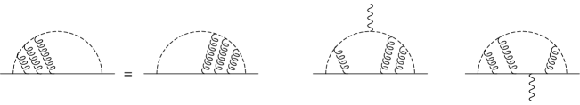
(a)                                                (b)                        (c)

Figure 15: A typical member of the self-energy graphs is shown in (a). Typical members of the $\gamma$MBB vertex, obtained by inserting one photon into the graph (a), are shown in (b) and (c).

can be lumped as dressing of one of the two bare vertices. The ladder cannot be split to dress both vertices.

The $\gamma$MBB vertex graphs are obtained by inserting one photon in all possible ways in every self-energy graph. Figs 15(b) and (c) are two examples. When we consider all such graphs, it is clear that the ladders can be lumped into dressing the left and the right vertices giving rise

Figure 16: Proton strangeness vertex diagrams following from the dressing of the KP$\Lambda$ vertex with a complete set of ladders of $\sigma$ exchange. The MBB vertex is defined in Fig. 8 and the seagull term in Fig. 9.

to the two dressed graphs of Fig. 16. There are no seagull terms in Fig. 16, which is in sharp contrast to the result of the Ohta approach described by Fig. 11.

In reality the KP$\Lambda$ vertex will be dressed not simply by a complete set of ladders but in various other ways. Many of these will generate seagull terms which are the same as those occurring in the corresponding $\gamma$MBB vertex for the particular form of dressing. At the same time the dressing by a complete set of ladders is manifestly an important process. Thus we can assert that the seagull terms which occur in the calculation of proton strangeness content are not the same as those which occur in the $\gamma$KP$\Lambda$ vertex. A complete knowledge of the algebraic form of the $\gamma$KP$\Lambda$ vertex will not enable us to predict the seagull terms which may occur in the proton strangeness content calculation. In other words Ohta’s prescription does not work in a general loop graph.

6 Results and Conclusions

It has been known for some time that baryon electromagnetic amplitudes have problem with gauge invariance if meson-baryon form factors are used.

Recognizing these difficulties Ohta [2] tackled the problem of Ward-Takahashi identity for $\gamma$MBB vertex in terms of MBB vertex by first introducing a dynamical basis. Given a MBB vertex, he wrote down an interaction Lagrangian which gave the specified vertex at the tree level. The electromagnetic interaction was introduced via minimal substitution ensuring that the resulting $\gamma$MBB vertex would satisfy the Ward-Takahashi identity. The novel features of his result was (a) the appearance of a seagull term determined entirely by the MBB vertex and (b) that the seagull term is robust, i.e. it appears unchanged in other electromagnetic amplitudes.

It is important to note that the transverse part of the $\gamma$MBB vertex is not fixed by this procedure as it is not constrained by considerations of Ward-Takahashi identity.

We demonstrate that an interaction Lagrangian which generates the MBB vertex function at tree level cannot be either hermitian or invariant under charge conjugation. Yet we find that Ohta’s discovery of the presence of a seagull term in the photo-meson amplitude is correct and its algebraic relation with the meson-baryon vertex function is also correct. Most importantly, we find that this result is totally independent of any details of the dynamics. Specific knowledge of the Lagrangian is not needed.

Unfortunately, we also find that, in general, the resulting seagull term is not robust. A loop graph of an electromagnetic amplitude will contain a seagull term if a meson baryon form factor has been used, but it will not be the same as that appearing in a photo-meson amplitude. This point was established with the help of a gauge-invariant subset of graphs which describes the dressing of the meson-baryon vertex with a complete set of ladders of $\sigma$-exchange. In this case while there is a seagull term in the photo-meson amplitude, there is none in the loop graph for charge radius or strangeness content.

The seagull terms always act in a robust manner in exchange current graphs.

The problem of gauge invariance in calculations with meson-baryon form factors is very important, particularly, in view of the proposed experiments at the Jefferson Lab to measure the strangeness content of proton. It is unfortunate that Ohta’s clever prescription turns out not to be quite correct. Obviously more work is needed to come up with a constructive proposal to solve the problem in a gauge invariant manner. This may require some approximations in handling the strong interaction dynamics.

References

[1] S. Weinberg, Physica A96 (1979) 327; J. Gasser and H.
Leutwyler, Phys. Rep. 87 (1982) 77.
[2] K. Ohta, Phys. Rev. C40 (1989) 1335.
[3] M.J. Musolf, M. Burkardt, Z. Phys. C61 (1994) 433.