Dimensional Power Counting in Nuclei

Abstract

Weinberg’s dimensional power counting for nuclei is reprised in this primer. The role of QCD and chiral symmetry in constructing effective Lagrangians is discussed. The two-scale hypothesis of Manohar and Georgi is combined with power counting in amplitudes to shed light on the scales of nuclear kinetic and potential energies, the size of strong-interaction coupling constants, the size of meson-exchange currents, and the relative sizes of $N$-nucleon forces. Numerous examples are worked out and compared to conventional nuclear models.

1 Nuclear Perspectives

What is a nucleus and what are its constituents? This question has no direct answer, or even a unique one. Indeed, the proper answer depends on the context of the question. Alternatively, the answer depends on the energy scale at which we are probing the nucleus. At extremely high energies such as those of CERN or RHIC, we might suppose that the appropriate degrees of freedom (d.o.f.) are quarks and gluons. At very low energies (such as nuclear ground states), the more natural degrees of freedom would be nucleons and possibly pions. After all, collisions of a nucleus with low-energy projectiles ($\sim$ tens of MeV) eject nucleons. This traditional description of a nucleus as interacting nucleons would seem at first glance to have little direct connection with QCD, the fundamental theory of the strong interactions. The former description in terms of quarks and gluons obviously has such a connection, since the beautiful economy and symmetry of the theory is manifest in terms of these d.o.f[1, 2].

A close connection between the two descriptions must exist, but it is murky. The traditional picture of nuclei has been very successful, provided that the complexities of the short-range nuclear force are resolved by appeal to experiment. While this works for the nucleon-nucleon ($NN$) force[3], we have as yet been nearly powerless to resolve the three-nucleon force in this way, although substantial progress is being made[4]. The few-nucleon systems are arguably the area of nuclear physics where the most progress has been made on seminal problems during the previous decade or so[5]. We expect (and will see) that these systems do provide us with substantial information on dynamics, assuming that we can interpret it. That is the purview of this article. Conversely, the scheme that is outlined below has the potential to augment greatly our understanding of nuclear dynamics, and particularly the role and appreciation of few-nucleon systems (our testing ground) in this endeavor.

Traditional nuclear physics is the domain of large coupling constants (the interaction is strong), which presupposes that perturbation theory cannot converge. Although we will see below that this is true in part, it is not true in toto, and this caveat makes progress possible. Connections to QCD (at least the qualitative ones) are easy to make and most are long known[1, 2], and follow from the chiral symmetry (CS) manifested by QCD.

$\bullet$ The pion has a very small mass, $m_{\pi}$.

$\bullet$ The pion is a pseudoscalar particle ($J^{\pi}=0^{-}$).

$\bullet$ The pion is an isovector particle.

$\bullet$ Chiral symmetry forbids large $\pi N$ interactions.

$\bullet$ There is a large-mass scale, $\Lambda\sim$ 1 GeV, associated with QCD.

The first four items involve the pion and are extremely important, but have been known for decades[6]. The last item is new[1, 7, 8], and its consequences for nuclear physics are more subtle and will shape the contents of this article. In the past, the lack of any apparent dynamical scales in nuclear physics made progress in interpreting results rather difficult.

The (broken) chiral symmetry referred to above is a consequence of (nearly) massless quarks in the QCD Lagrangian. This symmetry is reflected in the Goldstone mode by (nearly) massless pions[8]. An analogous chiral symmetry exists in QED if the electron mass is set to zero; this symmetry produces a vanishing amplitude for (relativistic) electrons scattering backwards from the nuclear charge distribution. The very small pion mass plays a significant role in nuclear physics, producing the longest-range part of the strong force. The pseudoscalar nature of the pion guarantees a spin-dependent interaction with a nucleon, and this leads to the tensor force, the dominant component[9] of binding in few-nucleon systems ($\langle V_{\pi}\rangle/\langle V\rangle\sim$ 75%) and possibly in all nuclei. The existence of charged pions guarantees them a large role in electromagnetic (EM) meson-exchange currents[10], which we will treat later. The fourth item on the list is critical for a tractable theory of nuclei. It guarantees that a class of many-body forces is weak[11, 12] (we will see later that they all are weak). Item five allows us to combine phenomenology with principle, and is the organizing element of Chiral Perturbation Theory ($\chi$PT)[1, 2, 13, 14, 15], which we will treat qualitatively. It is not unreasonable to expect that this subject will become increasingly important to nuclear physics in the next decade, and this primer was motivated by that supposition.

As evidence for these views, Table 1.1 shows the (current) results of one of the most important (set of) calculations undertaken in nuclear physics[16]. Using the best available $NN$ force, a weak three-nucleon force (3NF), and no four-nucleon force (4NF), the light nuclei ($A\leq 6$) were calculated with an uncertainty $\mathrel{\raise 3.0pt\hbox to8.0pt{\raise-6.0pt\hbox{$\sim$}\hss{$<$}}}$ 1%. The agreement with experiment must be considered very good. Our goal will be to understand these results in simple terms.

Table 1: Calculated and experimental ground-state energies (in MeV) of few-nucleon systems, together with (approximate) dates when they were first accurately solved for “realistic” potentials.

${}^{\rm A}{\rm X}(J^{\pi})$	${}^{2}{\rm H}(1^{+})$	${}^{3}{\rm H}(\frac{1}{2}^{+})$	${}^{4}{\rm He}(0^{+})$	${}^{5}{\rm He}(\frac{3}{2}^{-})$	${}^{5}{\rm He}(\frac{1}{2}^{-})$	${}^{6}{\rm Li}(1^{+})$
Solved	$\sim$1950	1984	1987	1990	1990	1995
Expt.	-2.22	-8.48	-28.3	-27.2	-25.8	-32.0
Theory	-2.22	-8.47(2)	-28.3(1)	-26.5(2)	-25.7(2)	-32.4(9)

We summarize this discussion by stating that

$\bullet$ Chiral Symmetry (manifested in QCD) provides an organizing principle for nuclear physics.

2 Motivation

In 1979, Weinberg[8] suggested that a convenient and simple way to reproduce the results of current algebra (and go beyond) was to use a nonrenormalizable, phenomenological Lagrangian that manifests chiral symmetry. Such a scheme would produce amplitudes of the form: $T\sim$ $E^{\nu}$, where $E$ is the energy. This was obtained using dimensional analysis and specified $\nu$ to be an integer determined by the type of process and by chiral symmetry. The constraints of CS mandate that more complicated mechanisms necessarily have larger values of $\nu$. Thus, provided that $E$ is smaller than some intrinsic energy scale, $\Lambda$, one has a decreasing series (i.e., it is a series in $E/\Lambda$) that is calculable. This series is organized in terms of $\nu$ rather than around unspecified (large) coupling constants. For this to work effectively $\Lambda$ must be sufficiently large, and more complicated mechanisms must not produce smaller values of $\nu$. That is, amplitudes from loops and other products of higher-order perturbation theory (PT) should not be larger than lower orders. As noted by Weinberg, the derivative structure of his Lagrangian (which enforced CS) guarantees this. Concomitant with the nonrenormalizability was the appearance of more and more unknown constants at higher orders in PT, which must be determined from experiment or calculated from QCD. This feature clearly is a drawback, and one hopes that meaningful results can be obtained before the number of terms becomes too large for tractability.

This seminal, but skeletal, argument was developed into a highly successful program by the Bern group (and others)[17] who introduced fermions. A very important addition to the counting argument was made by Manohar and Georgi[7], which we will discuss later. Much later (in a series of papers) Weinberg[11] applied the procedure to nuclei. Different terse versions of the counting were constructed in the various papers, while adapting the argument to the nuclear environment, a nontrivial achievement. This was extended in several ways in the thesis of van Kolck[12], which is an excellent introduction to those aspects of the problem that we will ignore.

Our task is to reprise the derivation of Weinberg, add expository material familiar to nuclear physicists in order to make the results concrete, and finally to extract a number of crisp conclusions with import for nuclear physics and especially for the few-nucleon field. It can be fairly stated that there is nothing in this primer that is not stated or implied in the work of Weinberg, van Kolck, and others. Nevertheless, the importance of these ideas and their unfamiliarity to our field make an exposition desirable. We will see that many qualitative results follow from simple arguments, once the framework has been constructed.

In order to satisfy the whims of the author, an older alternative form of power counting (the “rules of scale”[18, 19]) will also be separately presented. Although this has been in use for decades[20], it is inappropriate for such complex mechanisms as loops and, moreover, it has no grounding in chiral symmetry. It is, however, rather simple minded, easy to use, and does generate some insight into the nuclear physics that is less visible in the more formal approach.

Finally, we will fashion all of our arguments around Feynman diagrams, so we assume that the reader has some familiarity with their structure[21]. Specific examples with regularization and renormalization are relegated to Appendices B and C. The first example illustrates a number of currently popular techniques and approaches, while the second treats a simple two-nucleon problem. An exposition of nuclear matrix elements in momentum space is extremely helpful in interpreting the power counting in nuclei, and is relegated to Appendix A. Otherwise, we will attempt to motivate the physics as we proceed.

We will show the following results at various points in the primer:

$\star$ The kinetic energy/nucleon scales as $Q^{2}/\Lambda$, where $Q$ is an effective momentum in the nucleus.
$\star$ The “intrinsic” potential energy/pair scales as -$Q^{3}/f_{\pi}\Lambda$, where $f_{\pi}$ is the pion-decay constant.
$\star$ The cancellation of these two comparable energies allows nuclei to be weakly-bound systems ($\langle T\rangle\sim-\langle V\rangle$ and binding energy $\ll$ mass).
$\star$ Large strong-interaction coupling constants are caused by the mismatch between the $f_{\pi}$ and $\Lambda$ scales.
$\star$ $N$-nucleon forces decrease in strength as $N$ increases. This powerful result authenticates decades of nuclear physics supposition and phenomenology.
$\star$ Increasingly more complicated forces contribute more weakly.
$\star$ Arbitrary processes contribute to the energy as $Q^{\nu}$, where $\nu=1+2(n_{c}+L)+\Delta$, with $L$ the number of loops, $n_{c}$ a topological parameter, and $\Delta\geq 0$ reflects the complexity of the interaction. This is Weinberg power counting.

3 Rules of Scale - Nuclear Methodology

A type of primitive power counting has been in use for two decades[18, 19, 20]. The “rules of scale” were developed as a way to control expansions that arise in nonrelativistic treatments of meson-exchange currents. Specifically, expansions in powers of $1/c^{2}$ were organized by noting that the velocity of a typical nucleon (with mass $M_{N}$ and momentum $p$) is $v=p/M_{N}$, and consequently $v/c\sim p/M_{N}\,c$. Thus, counting powers of $1/M_{N}$ in an expansion is equivalent to counting powers of $1/c$. It was noted that nuclei are weakly bound, implying that the kinetic and potential energies satisfy $\langle T\rangle\sim-\langle V\rangle$. Hence, $V$ should be counted as $1/M_{N}$, since $V\sim T\sim p^{2}/2M_{N}$. This scheme works well at “tree” level (i.e., those mechanisms that don’t involve loops, which were typically of interest in those times) and, more importantly, it works for the current continuity equation, which is essential for EM processes. That is, consistency in that equation demands that energies of all types be treated on the same footing. Conversely, the scheme has no predictive power for loops.

In order to progress further, we need some indication that $v/c\ll 1$. Otherwise, the Schrödinger approach is meaningless. We can use the uncertainty principle and the radii[23] of the few-nucleon systems ($\sim$ 1.5 - 2.0 fm) to produce: $pc\sim\hbar c/R\sim$ 100-150 MeV $\sim m_{\pi}c^{2}$, where the last relation is a convenient mnemonic, rather than a statement of principle, since $m_{\pi}$ (unlike $f_{\pi}$, for example) vanishes in the chiral limit. This leads to

$$v/c\sim p/M_{N}c\sim m_{\pi}/M_{N}\sim 10-20\%\,,$$

and $(v/c)^{2}$ is satisfyingly small on average. In order to conform to a more standard notation, we will use $Q\,(\sim m_{\pi})$ rather than $p$. We will see later that in processes involving pions this is indeed a typical scale[24].

At this point a little history is instructive. There are at least three ways of organizing the interactions of pions with nucleons. This familiar argument has been distracting and ultimately unproductive (the author has been guilty of this[19, 20, 25]), but it illustrates a number of useful points. Parity and time-reversal-invariance arguments allow the Lagrangian for a single pion-nucleon interaction to be either

$${\cal{L}}_{\pi NN}=-iG\bar{N}\gamma_{5}\mbox{\boldmath$\tau\cdot\pi$}N\,,$$

or

$${\cal{L}}^{\prime}_{\pi NN}=-\frac{f}{m_{\pi}}\bar{N}\gamma_{5}\hbox to0.0pt{$\partial$\hss}/(\mbox{\boldmath$\tau\cdot\pi$})N\,,$$

where $f=Gm_{\pi}/2M_{N}$. These two forms are usually referred to as PS (pseudoscalar) and PV (pseudovector). An alternative form is introduced by using the Goldberger-Treiman[26] relation:

$$\frac{G}{M_{N}}=\frac{g_{A}}{f_{\pi}}\,,$$

where $G\simeq 13,g_{A}\simeq 1.26$ is the axial-vector coupling constant and $f_{\pi}\simeq 92.4$ MeV is the pion-decay constant. This remarkable relationship (the author’s favorite in strong-interaction physics) relates strong interactions on the left side to weak interactions on the right, and is violated at the level of 2% [27] by chiral-symmetry breaking (the left side is larger). Thus we can also rewrite Eq. (3.3) by replacing $f/m_{\pi}$ with $g_{A}/2f_{\pi}$, generating the third and preferred form

$${\cal{L}}^{\prime\prime}_{\pi NN}=-\frac{g_{A}}{f_{\pi}}\bar{N}\gamma_{5}\hbox to0.0pt{$\partial$\hss}/(\mbox{\boldmath$t\cdot\pi$})N\,,$$

where we have written $t$ = $\tau$/2 (a very common practice).

Note the very different sizes of the interactions in Eqs. (3.2) and (3.3): $G\sim 13$, while $f\sim 1$. These two forms are equivalent on-shell, but differ dramatically off-shell. We will see later that the off-shell behavior is controlled by chiral symmetry through terms we have not explicitly written. In particular the large $N\bar{N}$-“pair” terms implicit in the first form are exactly cancelled, a phenomenological result known historically as “pair suppression”. These pair terms have a very large dimensionless strength, $G^{2}m_{\pi}/M_{N}\sim 25$, producing many-body forces that would make the tractability of nuclear physics problematic. The large size of $G$ is typical of the strong interactions, while $f$ is much more modest. Even more modest is the effective coupling constant for the one-pion-exchange potential (OPEP) shown in Fig. (1a). This amplitude, when converted to configuration space, generates a factor of $1/4\pi$, whose precise form depends on the fact that we live in three space dimensions (see Appendix B):

$$\int\frac{d^{3}q}{(2\pi)^{3}}\frac{e^{i\mbox{\boldmath$q\cdot r$}}}{\mbox{\boldmath$q$}^{2}+m^{2}_{\pi}}=\frac{m_{\pi}}{4\pi}\left[\frac{e^{-m_{\pi}r}}{m_{\pi}r}\right]\,.$$

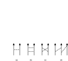
Figure 1: One- and two-pion-exchange contributions to the nuclear force. Solid lines are nucleons, while dashed lines are pions.

Rendering OPEP[9] into a dimensionless radial function of ${\bf x}=m_{\pi}{\bf r}$ and an overall dimensionful factor, we have $V_{\pi}(\mbox{\boldmath$r$})\equiv\frac{m_{\pi}^{3}g_{A}^{2}}{4\pi f_{\pi}^{2}}V(\bf{x})$. Obviously some care is required in this exercise, since $4\pi$ is dimensionless. It is, however, a large number and we extract it. We expect $\langle V({\bf x})\rangle\sim 1$ since $\langle 1\rangle\equiv 1$, where $1$ is the unit operator (this is our normalization convention) and because correlations with a length $\sim 1/m_{\pi}$ are introduced into the wave function by $V(x)$. This implies that values of x near 1 are very important (which can be verified in Fig. (7)) and our functions near $x=1$ are ${\cal O}$(1) [cf., Eq. (3.6)]. The net result is that we expect a pair of nucleons exchanging a pion to generate an energy $\sim m_{\pi}^{3}g_{A}^{2}/4\pi f_{\pi}^{2}\sim$ 20 MeV. Anticipating a result from Section 5 and Appendix B, we note that $4\pi f_{\pi}\sim$ 1200 MeV $\sim\Lambda$, where $\Lambda$ was introduced in Section 1. Recalling $Q\sim m_{\pi}$, we obtain $\langle OPEP\rangle\sim\frac{Q^{3}}{\Lambda f_{\pi}}C_{V}$ per pair, where $C_{V}$ is the product of all the dimensionless factors $\sim 1$ (by supposition). We have already argued that $\langle T\rangle\sim\frac{Q^{2}C_{T}}{\Lambda}$ per nucleon, where $C_{T}\sim 1$ and we have used $M_{N}\sim\Lambda$. For the triton, $\langle V_{\pi}\rangle\sim-15$ MeV/pair and $\langle T\rangle\sim 15$ MeV/nucleon[24]. For the $\alpha$ particle both energies are somewhat larger. In heavier systems, where the Pauli Principle begins to play a large role, these numbers (particularly the potential energy) cannot be correct. Nevertheless, the “intrinsic” scale for these quantities is

$$\langle T\rangle/{\rm nucleon}\sim Q^{2}/\Lambda\,,$$

$$\langle V_{\pi}\rangle/{\rm pair}\sim\frac{-m^{3}_{\pi}}{(4\pi f_{\pi})f_{\pi}}\sim\frac{-Q^{3}}{\Lambda f_{\pi}}\sim\frac{-Q^{2}}{\Lambda}\,,$$

confirming that kinetic and potential energies (and quantities derived from them, such as impulse-approximation and meson-exchange EM currents) should be counted similarly (numerically, $Q\sim f_{\pi}$), in the absence of large dimensionless coefficients that would skew the similarity. Thus, for OPEP and light nuclei we see a confirmation of the weak-binding hypothesis that formed the basis for the rules of scale. Moreover, the numerical results based on calculations with realistic potentials are consistent with these scales.

Two other potentials have been calculated that can be similarly analyzed. Figures (1b) and (1c) show various parts of the two-pion-exchange potential (TPEP). These Feynman graphs can be separated into two components: an intrinsic TPEP and the simple iteration of OPEP (which happens automatically whenever the Schrödinger equation is solved). The “intrinsic” size of the former is[25]

$$\langle TPEP\rangle\sim\frac{m_{\pi}^{5}}{(4\pi f_{\pi})^{3}f_{\pi}}\sim\frac{Q^{5}}{\Lambda^{3}f_{\pi}}\sim\frac{1}{2}\,{\rm MeV/pair}\,.$$

Two-pion-exchange three-nucleon forces ($2\pi E3NF$) can be similarly analyzed[19] (see Fig. (1d)):

$$\langle 2\pi E3NF\rangle\sim\frac{m^{6}_{\pi}}{M_{N}(4\pi f_{\pi})^{2}f^{2}_{\pi}}\sim\frac{Q^{6}}{\Lambda^{3}f^{2}_{\pi}}\sim\frac{3}{4}\,{\rm MeV/triplet}\,.$$

In counting arguments of this type, we have avoided factors of $g_{A},2,1/2$, etc., and hope that they average out $\sim$ 1. In most cases, they do (within an overall factor of 2). In Sections 6, 8, and 9, we will derive a very simple formula (Weinberg’s formula) that reproduces all of these results by power counting (in $Q$ and $1/\Lambda$) with almost no effort.

The only remaining problem is Fig. (1b). This diagram, unlike a typical case, does not have momenta $\sim Q\sim m_{\pi}$ flowing through every propagator. Indeed, after the first interaction the propagator is typically $(E-T)^{-1}\sim(p^{2}/2M_{N})^{-1}\sim M_{N}/Q^{2}$. Graphs of this type are called “reducible”. The small-$Q$ or “infrared” singularity enhances the graph by a factor $\sim M_{N}/m_{\pi}$ compared to a typical case. This singularity is also the origin of the “ambiguity problem”[19, 20, 25], which reflects the fact that a potential is an off-shell amplitude, and hence is not unique. The dichotomy between these two types of graphs (reducible and irreducible) greatly reinforces the case for the following calculational scenario:

$\diamond$ Calculate irreducible graphs (where simple power counting works) and define this as the nuclear potential.

$\diamond$ Solve the Schrödinger equation with that potential – the infrared enhancements will happen automatically.

On the basis of several examples (this does not in any sense constitute a proof, which will follow in Section 6) we find that

$\bullet$ Various nuclear energies behave as $Q^{\nu}/\Lambda^{\nu-n_{c}-1}f^{n_{c}}_{\pi}$ for some values of $\nu$ and $n_{c}$, with more complicated mechanisms generating larger values of $\nu$. We have used $\Lambda\sim 4\pi f_{\pi}\sim M_{N}$ in this simple counting exercise.

4 Effective Interactions

The basic idea is a simple one. Strong-interaction physics can be divided into two parts: short-range (high-energy) parts and long-range (low-energy) parts. We hope that the former is not dominant, but it could be. This is the most difficult domain of nuclear physics, where phenomenology reigns supreme. The long-range physics is of two (nonexclusive) types: (1) from pion-range physics, and (2) from iterations of the nuclear potential, as we saw in the previous section. Even though convergence requirements restrict us to the low-energy regime, it is essential that the pion degrees of freedom be treated explicitly; they have a strong energy dependence even at low energy. We also saw that the infrared singularity that results from iterating the potential plays a very important role in nuclear physics.

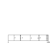
Figure 2: Unflavored meson spectrum [plus $\Delta$-isobar excitation energy] below 1 GeV.

The short-range regime is where all the complexity of QCD resides. Consider, for example, the unflavored meson spectrum below 1 GeV, plotted in Fig. (2). Only two mesons lie below 770 MeV: $\pi$ and $\eta$. In an SU(3) (rather than SU(2)) treatment of the chiral symmetry (i.e., strangeness is included), we would treat the ($\pi,\eta,K$)-meson octet together. Although the $\eta$-meson contribution to the nuclear force is not particularly important, in an SU(2) approach its low mass would be problematic for the formalism. The other (heavy) mesons have masses $\geq$ 770 MeV. We can therefore imagine a scheme where the effect in appropriate spin and isospin channels of all single and multiple heavy-meson exchanges, loops, $\ldots$ is “frozen out”[15]. That is, the effects of all possible short-range mechanisms are lumped together without regard to their origin. This is accomplished by noting that (for low energies) a derivative expansion about the zero-range limit is formally possible. Thus $\Lambda\sim m_{\rho}\sim$ 1 GeV is also the boundary between the short-range and long-range physics.

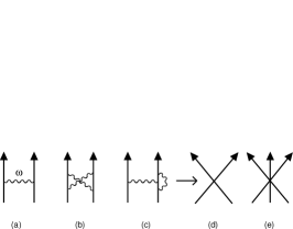
Figure 3: $\omega$-meson contributions in (a-c) to short-range $NN$ force in (d), plus an additional 3NF in (e). Solid lines are nucleons, while wavy lines are $\omega$ mesons.

Figure (3) illustrates this approach, where a few selected mechanisms involving $\omega$ mesons are shown. All are subsumed in (3d), which is the sum of various zero-range interactions that can include derivatives. As an example, we treat Fig. (3a), for which the S-matrix is given by

$$S=-ig^{2}_{\omega}\frac{(\bar{u}_{1}\gamma_{\mu}u_{1})(\bar{u}_{2}\gamma^{\mu}u_{2})}{q^{2}-m^{2}_{\omega}}\,,$$

where we follow the conventions and metric of Ref. [21]. We have dropped normalization factors and the overall four-momentum-conserving factor, $(2\pi)^{4}\delta^{4}(P_{1}+P_{2}-P_{1}^{\prime}-P_{2}^{\prime})$, for this two-nucleon cluster. The strong coupling of the $\omega$ (with mass $m_{\omega}$) to the nucleon is reflected by the coupling constant, $g_{\omega}$, the nucleons (with spinors, $u$) have been arbitrarily labeled “1” and “2”, and $q^{\mu}$ is the momentum transferred in the collision ($q^{2}<0$). We now expand the denominator for $-q^{2}\ll m^{2}_{\omega}$

$$\frac{1}{m^{2}_{\omega}-q^{2}}\simeq\frac{1}{m^{2}_{\omega}}+\frac{q^{2}}{m^{4}_{\omega}}+\cdots\,,$$

and define each term in the series as a new effective interaction (Lagrangian)

$$S\simeq i\left(\frac{g^{2}_{\omega}}{m^{2}_{\omega}}\right)(\bar{u}_{1}\gamma_{\mu}u_{1})(\bar{u}_{2}\gamma^{\mu}u_{2})(1+\frac{q^{2}}{m^{2}_{\omega}}+\cdots)\,,$$

leading to (see Ref. [22])

$${\cal{L}}_{eff}={\cal{L}}^{(0)}_{eff}+{\cal{L}}^{(2)}_{eff}+\cdots\,,$$

$${\cal{L}}^{(0)}_{eff}=\frac{1}{2}\left(\frac{g^{2}_{\omega}}{m^{2}_{\omega}}\right)(\bar{N}\gamma_{\mu}N)^{2}\,.$$

We have defined the effective Lagrangian so that the usual Feynman rules produce, term-by-term, the same S-matrix. We have added a superscript to $\cal{L}$, $``\Delta"=0,2,4,\ldots$, that serves the same purpose as Weinberg’s $``\nu"$ that we introduced earlier. It classifies the interaction here according to powers of $q$; we will develop the rules later for this notation. More complicated short-range forces are possible, as indicated by the three-nucleon force in Fig. (3e).

We have used the fact that the $\omega$ meson is sufficiently heavy that (for small $q^{2}$) it propagates only a very short distance between emission and reabsorption (à la the uncertainty principle)[28]. Since we have assumed a particular mechanism, we have developed a model for the strength of the zero-range interaction. Unfortunately, a vast array of mechanisms including but not restricted to Figs. (3a) - (3c) (viz., loops to arbitrary order, physics not involving the $\omega\ldots$) also contribute. Thus, this coefficient (and others with $\Delta>0$) is unknown and must be determined phenomenologically or calculated directly from QCD.

Two more aspects are important and somewhat controversial. In addition to mesons being “exchanged”, we also have to consider nucleon resonances. Figure (2) shows the $\Delta$-isobar excitation energy superimposed on the meson spectrum. The low excitation energy of the $\Delta$ has long stimulated the imagination of nuclear theorists, and mechanisms proposed for almost every nuclear effect will typically include a $\Delta$ somewhere. The uncertainty principle states that the virtual excitation of a $\Delta$ scales inversely with the $\Delta$ energy (i.e., as $1/E_{\Delta}$). Recent work suggests that in some regimes (viz., three-nucleon forces and meson-exchange currents[29]) $E_{\Delta}$ behaves more as $\Lambda\sim$ 1 GeV than $M_{\Delta}-M_{N}\sim$ 300 MeV. In other regimes (threshold $pp\rightarrow pp\pi^{0}$, for example[30]) the opposite is more likely. In constructing effective interactions, some theorists[12] routinely include the $\Delta$ in the active Hilbert space, while others do not. Care should be taken when assuming that the $\Delta$ is not very important. We will, however, ignore the $\Delta$ in what follows solely for reasons of simplicity.

The second aspect concerns relativity. The simple example involving the $\omega$ meson respected special relativity, including the derivative terms ($\sim q^{2}$). More complex mechanisms would lead to terms proportional to the overall momentum $p^{\mu}$ of a nucleon, rather than the momentum transfer, $q^{\mu}$. While the latter is typically not large, $p^{\mu}=(E,\mbox{\boldmath$p$})$, and $E\sim M_{N}\sim\Lambda$ is large. This would lead to a series of terms that would all be the same size (recall that we have a series in $E/\Lambda$). The problem can be formally eliminated by performing a $1/M_{N}$ expansion (e.g., a Foldy-Wouthuysen reduction[20, 21]), where the effect of $N\bar{N}$ “pair” terms is projected out, and one treats only the positive-energy spectrum. This “freezing out” of degrees of freedom is familiar to nuclear physicists in the Feshbach (P-Q) reaction theory[32], where the Hilbert space is compacted from the normal to a restricted size, leading to much more complex operators (which must reproduce the physics of the larger Hilbert space in the smaller one). Covariance is lost, but one retains an expansion in $Q$, rather than introducing terms $\sim M_{N}$ at every order. This alternative formalism is given the generic name “heavy-baryon” and is currently the method of choice[33, 34]. This presupposes that a nonrelativistic treatment of the nuclear physics is appropriate, which clearly holds for the few-nucleon systems. We give an example of a nonrelativistic loop calculation in Appendix B, and compare it to a relativistic one. Appendix C treats a simple nonrelativistic two-nucleon model.

We summarize this section by noting that:

$\bullet$ The complexities of strong-interaction physics can be divided into long-range and short-range parts, with pion d.o.f. dominating the former and the latter condensed into zero-range interactions of unknown size.

$\bullet$ Effective interactions are constructed by “freezing out” the short-range degrees of freedom (mesons, resonances, $N\bar{N}$ pairs, $\ldots$), leading to structurally more complex interactions that (hopefully) are easier to treat at low energies.

$\bullet$ The $\Delta$ isobar can be included in the active Hilbert space (with the pions) or not, depending on the problem to be solved.

$\bullet$ A nonrelativistic, nonrenormalizable field theory is possible to construct and to use.

5 Dimensional Power Counting in Lagrangians

We begin by considering the dimensions of various quantities in order to assess the scales of the strong interactions. Our approach in this section will be to motivate rather than to attempt rigor. The interested reader should consult Refs. [1, 7, 8] for a more sophisticated approach. We will also formulate the arguments supposing a relativistic field theory. Following the discussion of the previous section, they also apply mutatis mutandis to a nonrelativistic “heavy-baryon” field theory.

We denote a power $\nu$ of energy by $[E^{\nu}]$ (equivalent to $length^{-\nu}$), and recall that a Lagrangian has dimension 4 (i.e., behaves as $[E^{4}]$). The Lagrangian for a system of pions and nucleons interacting through derivatives ($\partial^{\mu}$) acting on any field can be written in the schematic form

$${\cal{L}}={\cal{L}}_{free}+\Delta{\cal{L}}\,,$$

$${\cal{L}}_{free}=\bar{N}(i\gamma_{\mu}\partial^{\mu}-M_{N})N+\frac{1}{2}(\partial^{\mu}\mbox{\boldmath$\pi$})^{2}-\frac{1}{2}m^{2}_{\pi}\mbox{\boldmath$\pi$}^{2}\,,$$

$$\Delta{\cal{L}}\sim a\left(\frac{\bar{N}(\cdots)N}{b}\right)^{\ell}\left(\frac{\mbox{\boldmath$\pi$}}{c}\right)^{m}\left(\frac{\partial^{\mu}}{d}\right)^{n}\,.$$

The combination $\bar{N}N$ has dimension $[E^{3}]$, while $\pi$ and $\partial^{\mu}$ (as well as $m_{\pi}$ and $M_{N}$) have dimension $[E]$, and $\Delta{\cal{L}}$ of course has dimension $[E^{4}]$.

Our first assumption is that only the scales $f_{\pi}$ and $\Lambda$ occur in $a,b,c,d$ and also that $\Delta{\cal{L}}$ should reproduce ${\cal{L}}_{free}$. Clearly, $c$ must be $f_{\pi}$, since that quantity sets the scale for the pion field (cf., PCAC[1, 2, 6, 21]). Setting $\ell=0$ and $m=n=2$ gives $a/c^{2}d^{2}\sim 1$, while $m=0,\ell=1$, and $n=0,1$ give $a/b\sim\Lambda$ and $a/bd\sim 1$ (where we have substituted $M_{N}\sim\Lambda$). These three equations can be uniquely solved to produce $d\sim\Lambda,a\sim f^{2}_{\pi}\Lambda^{2}$, and $b\sim f^{2}_{\pi}\Lambda$ and thus

$$\Delta{\cal{L}}=c_{\ell mn}\left(\frac{\bar{N}(\cdots)N}{f^{2}_{\pi}\Lambda}\right)^{\ell}\left(\frac{\mbox{\boldmath$\pi$}}{f_{\pi}}\right)^{m}\left(\frac{\partial^{\mu},m_{\pi}}{\Lambda}\right)^{n}f^{2}_{\pi}\Lambda^{2}\,,$$

where $c_{\ell mn}$ is dimensionless, and we have used the form of ${\cal{L}}_{free}$ to incorporate the chiral-symmetry-breaking pion-mass term into Eq. (5.4): a pion mass (either explicit or implicit) is treated as a derivative. All Dirac matrices, nucleon isospin operators, etc. have been ignored and are indicated by the dots.

This lovely formula has profound implications if we invoke chiral symmetry[8, 35]. No unique representation exists for incorporating chiral symmetry (cf., PS vs. PV forms), but a representation always exists in terms of covariant derivatives[1, 2, 8, 12], which has only increasing powers of ($1/\Lambda$). According to Eq. (5.4), these powers have the form $(1/\Lambda)^{\Delta}$, where

$$\Delta=n+\ell-2\,.$$

The minimum value for pions is $0$ from Eq. (5.2) and for nucleons is $-1$ for each of the two (largely) cancelling terms in Eq. (5.2) for free nucleons (i.e., $\gamma_{0}E-M_{N}$). This cancellation highlights the problem with derivatives of nucleon fields that we raised earlier: a slowly-moving nucleon actually has a kinetic energy, ${\cal{L}}_{free}=-N^{\dagger}\frac{\mbox{\boldmath$p$}^{2}}{2M_{N}}N$, or $\Delta=1$. The PV (derivative-representation) Lagrangian has $\Delta=0$. These examples motivate the rigorous result[8] that the derivative-representation chiral constraint has a form guaranteeing only positive powers of $1/\Lambda$ in Eq. (5.4):

$$\Delta\geq 0\,.$$

The PS form in Eq. (3.2) has $\Delta=-1$, which tells us that additional terms in the Lagrangian are required in order to construct a proper representation of chiral symmetry. Indeed, it was the neglect of the latter terms that led to the ad hoc “pair suppression” mechanism many years ago. This mechanism is automatic for chiral models or theories, as noted in many places. The use of a chiral representation corresponding to Eq. (3.2) requires an additional (leading-order) “pair”-killing interaction of the form[19]:

$$\Delta{\cal{L}}_{PS}=\frac{G^{2}}{2M_{N}}\bar{N}\mbox{\boldmath$\pi$}^{2}N\,.$$

We strongly argue that derivative forms be used, because the chiral constraint, Eq. (5.6), applies term-by-term.

The second assumption is that a reasonable theory should have[36]

$$c_{\ell mn}\sim 1\,,$$

or that the theory is “natural”. This is also called naive dimensional power counting (NDPC)[7, 35]. Clearly, if the scaling in Eq. (5.4) is a figment of our imaginations, the values of $c_{\ell mn}$ will jump all over. Verifying naturalness validates Eq. (5.4). We also note that if a symmetry exists, $c_{\ell mn}$ could be vanishingly small, but if the scaling hypothesis holds, very small coefficients would otherwise be just as unlikely as very large ones.

The third assumption is that vacuum fluctuations do not alter the scales that we introduced. It is shown in Refs. [1, 7] that it is necessary for loop integrals to be cut off at energies

$$\Lambda\mathrel{\raise 3.0pt\hbox to8.0pt{\raise-6.0pt\hbox{$\sim$}\hss{$<$}}}4\pi f_{\pi}$$

in order for the structure in Eq. (5.4) to be preserved, and we indeed have used $4\pi f_{\pi}\sim\Lambda$ interchangeably in Section 3 (see also Appendix B).

At this point, examples will serve us best in assessing the concept of “natural”, and to illustrate the use of Eq. (5.4). Evaluating that equation for $\ell=m=n=1(\Delta=0)$ and comparing it to Eq. (3.5) produces

$$c_{\pi}\sim g_{A}\sim 1.26\,.$$

Using $\mbox{\boldmath$\tau$}/2$ instead of $t$ would have produced the equally satisfactory $g_{A}/2$.

The zero-range $NN$ interaction produced by an $\omega$-meson exchange was derived earlier (Eq. (4.5)) and can be compared to the case $\ell=2,m=n=0$, yielding $c_{\omega}/f^{2}_{\pi}$ and a natural coupling constant

$$c_{\omega}\sim f^{2}_{\pi}\frac{g^{2}_{\omega}}{2\,m^{2}_{\omega}}\sim 1.75\,,$$

using the numerical entries in Table (A.2) of Ref. [37]. A famous example is the KSFR relation[38], which states

$$\frac{g_{\rho}}{m_{\rho}}\simeq\frac{1}{\sqrt{2}f_{\pi}}\,,$$

and corresponds to a zero-range Lagrangian: $\frac{g^{2}_{\rho}}{2m^{2}_{\rho}}(\bar{N}\gamma_{\mu}\mbox{\boldmath$t$}N)^{2}=\frac{1}{4f^{2}_{\pi}}(\bar{N}\gamma_{\mu}\mbox{\boldmath$t$}N)^{2}$ or $c_{\rho}\sim 0.25$. In general a heavy-meson exchange with mass $m_{x}$ and coupling constant (to the nucleon) $g_{x}$ corresponds to a zero-range Lagrangian with a coefficient, $\frac{g^{2}_{x}}{2m^{2}_{x}}\sim\frac{c_{x}}{f^{2}_{\pi}}$, implying that

$$g_{x}\sim\frac{m_{x}}{f_{\pi}}\sqrt{2c_{x}}\sim\frac{\Lambda}{f_{\pi}}\sim 10\,,$$

using $m_{x}\sim\Lambda$, and $\sqrt{2c_{x}}\sim 1$. This illustrates why strong-interaction coupling constants are large dimensionless numbers ($\sim 10$): the scales $\Lambda$ and $f_{\pi}$ are very different.

The next example of this type is a caution. What if there were a mechanism such as an $NN$ force component of normal size mediated by the exchange of a light meson $(m\ll\Lambda)$? This would correspond to a large value of $c_{x}$, and would likely lead in perturbation theory to a growing series whose structure violates Eq. (5.4). This is analogous to the intruder-state problem in nuclear-structure theory[39], where a low-energy state badly affects convergence of perturbation theory calculations. Another way of saying the same thing is that there would be another scale in the problem, which would violate the assumptions that led to Eq. (5.4).

We can also extend the NDPC to other forces. One isospin violation (IV) mechanism[12] is parameterized by the up-down quark-mass difference $m_{d}-m_{u}\equiv\epsilon\,(m_{d}+m_{u})$, where $\epsilon=(m_{d}-m_{u})/(m_{d}+m_{u})\sim 0.3$. The factor of $m_{d}+m_{u}$ is proportional to $m^{2}_{\pi}$[8] and Eq. (5.4) can still be used, provided that we identify[27]

$$c_{IV}\sim\epsilon\,c\,,$$

where $c$ is ${\cal O}$(1) and $n\geq 2$. That is, Eq. (5.4) has the $c_{\ell mn}$ replaced by $\epsilon\,c_{\ell mn}$, and there are at least two implicit powers of $m_{\pi}$. Similarly, parity-violating forces have $c$ replaced by[40]

$$c_{PV}\sim\frac{G_{F}\,f^{2}_{\pi}}{\sqrt{2}}\,c\,,$$

where $G_{F}$ is the Fermi constant and $c$ is ${\cal O}$(1).

Another application is the nuclear density, which for nuclear matter has the “empirical” value[41] $\rho_{\rm NM}=0.153\,{\rm fm}^{-3}\simeq 1.5f^{3}_{\pi}$. The generic Lagrangian contains powers of $\left(\frac{\bar{N}(\cdots)N}{f^{2}_{\pi}\Lambda}\right)$, the numerator of which is essentially the nuclear density $(N^{\dagger}N)$. At nuclear-matter density, the Lagrangian series (in $\ell$) is therefore geometric in $\frac{1.5f^{3}_{\pi}}{f^{2}_{\pi}\Lambda}=1.5f_{\pi}/\Lambda\sim 1/7$, which is comfortingly small, so that the expansion presumably works at normal nuclear density.

Our final example takes us outside the realm of few-nucleon systems. One might ask whether there have been any calculations performed using a Lagrangian of zero-range form. Although this has not been done in few-nucleon systems, there does exist one comprehensive Dirac-Hartree calculation[42] for a set of 57 nuclei using such forms (but without pion d.o.f). The various terms in the Lagrangian can be represented schematically by $\alpha(\bar{N}N)^{2}+\beta(\bar{N}N)^{3}+\gamma(\bar{N}N)^{4}+\delta(\partial^{\mu}\bar{N}N)^{2}$, where various isospin and Dirac matrices sit between $\bar{N}$ and $N$. A total of nine coupling constants were adjusted to fit the energies and radii of three representative nuclei. The results are among the best ever obtained for such a comprehensive set of nuclei. If one uses Eq. (5.4) with $m=0$ and various values of $\ell$ and $n$, and compares to the expressions in Ref. [42, 43], one obtains the results in Table (5.1).

Table 2: Optimized coupling constants for the Lagrangian of Refs. [42, 43] and corresponding dimensionless coefficients and chiral expansion order.

Constant	Magnitude	Dimension	${}c_{lmn}{}$	Order
$\alpha_{S}$	-4.508${\times}10^{-4}$	MeV-2	-1.93	$\Lambda^{0}$
$\alpha_{TS}$	7.403${\times}10^{-7}$	MeV-2	0.013	$\Lambda^{0}$
$\alpha_{V}$	3.427${\times}10^{-4}$	MeV-2	1.47	$\Lambda^{0}$
$\alpha_{TV}$	3.257${\times}10^{-5}$	MeV-2	0.56	$\Lambda^{0}$
$\beta_{S}$	1.110${\times}10^{-11}$	MeV-5	0.27	$\Lambda^{-1}$
$\gamma_{S}$	5.735${\times}10^{-17}$	MeV-8	8.98	$\Lambda^{-2}$
$\gamma_{V}$	-4.389${\times}10^{-17}$	MeV-8	-6.87	$\Lambda^{-2}$
$\delta_{S}$	-4.239${\times}10^{-10}$	MeV-4	-1.81	$\Lambda^{-2}$
$\delta_{V}$	-1.144${\times}10^{-10}$	MeV-4	-0.49	$\Lambda^{-2}$

The unscaled coupling constants (whose subscripts refer to Dirac and isospin matrices) span 13 orders of magnitude. Most of the scaled $c$’s that result are numbers near one. The average of the $\gamma$ terms is also natural. The uncomfortably large difference is possibly due to a lack of sensitivity in that quantity to the data. If the tiny value of $\alpha_{TS}$ is not an artifact of the fitting process or of the neglect of pion-range physics (unknown at this time) it presupposes a symmetry of some kind. Nevertheless, scaling as predicted by Eq. (5.4) is obvious. Improvements in the quality of the many-body techniques are not expected to alter this conclusion[43], but will alter each number.

We summarize this section by noting that:

$\bullet$ A two-scale hypothesis ($f_{\pi}$ and $\Lambda$) for the dimensional factors in the effective Lagrangian (plus chiral symmetry) suggests a convergent expansion of the Lagrangian series for normal nuclear conditions.

$\bullet$ This expansion has been organized so that vacuum fluctuations do not alter the form.

$\bullet$ The dimensionless coefficients in the Lagrangian are “natural” if they are ${\cal O}$(1), which we illustrated by several examples.

$\bullet$ Chiral symmetry guarantees that the large scale ($\Lambda\sim 4\pi f_{\pi}\sim m_{\rho}\ldots$) does not occur with positive powers.

6 Power Counting in Amplitudes

Power counting in amplitudes is a straightforward exercise, but somewhat tedious. It also is dependent on the environment and on what one chooses to emphasize. The result is worth the effort, however, since most of our previous results are subsumed by the very simple final forms. We work with nuclei, bound states of $A$ nucleons. Bound states are forever interacting, and one cannot simply separate interaction diagrams into connected and disconnected parts and discard the latter. Eventually each nucleon interacts and shares energy and momentum with the others. In normal (textbook) applications disconnected diagrams don’t contribute. We emphasize that the sharing of momentum dominates the systematics in a nucleus. The momentum that one nucleon takes from the “bank” is not available to the others.

The basic idea is to use our knowledge of the dimensionality of propagators, phase space factors, vertices, and delta functions to find the dimensionality of an amplitude, after eliminating all the coupling constants. Given this and knowledge of how the other scales (viz., $f_{\pi}$ and $\Lambda$) come into the problem, the coupling constants can be put back and a complete scheme can be constructed. We note that finding a momentum behavior $\sim Q^{\nu}$ does not necessarily imply a final $(Q/\Lambda)^{\nu}$ behavior. We also choose to work in configuration space, and this choice means that, while counting powers of momenta, the effect of additional phase space factors (besides those in loops) needed to convert to that space must also be incorporated, and this has been done in the derivation leading to Eq. (6.12). We will give examples later that spell out the differences, and Appendix A documents the various factors that normally arise. Finally, we postpone dealing with reducible (infrared-singular) diagrams until later. We first deal with the amplitudes, and then we will worry about the coupling constants.

Our first concern is what we should calculate and what rules apply. In general[20], the energy shift, $\Delta E$, in an interacting system is given in terms of the S-matrix (see Appendix B) by $S_{fi}\equiv\delta_{fi}-i\,\Delta E\;[(2\pi)^{4}\delta^{4}(P_{f}-P_{i})]$. The $\delta_{fi}$ factor for $N$ noninteracting particles is the product of three-momentum-conserving $\delta$-functions of each particle (see Eq. (6.35) of Ref. [21]) and behaves as $[E^{-3N}]$, while the energy shift (which is also the T-matrix) therefore behaves as $[E^{4-3N}]$. For a cluster of two nucleons ($N=2$) this has the dimensions $[E^{-2}]$, in agreement with Eq. (4.1) (the spinors and coupling constant in that equation are dimensionless). That form, as argued above, lacks the phase-space factor $\sim[E^{3}]$ needed to convert to configuration space. Together these factors produce $\sim[E]$, the correct dimension for an energy. We therefore use the same rules for an energy shift as for an S-matrix, stripping off the four-momentum-conserving $\delta$-function (if there is a single cluster) to produce $\Delta E$. Note that if there are $C$ separate clusters, there will be ($C-1$) cluster $\delta$-functions remaining to treat.

Our second concern is that there are many possible quantities that specify how momentum and energy flow in a given diagram. The key is to decide which ones to keep and which to eliminate. Typically one eliminates internal variables and keeps external ones. This is not enough for specificity and one additional choice remains. That choice will be made in such a way that the chiral constraint, Eq. (5.6), can be implemented by inspection. We also will calculate for fixed $A$, and eliminate at the end some extraneous factors that are dependent on our wave-function normalization scheme and depend only on $A$. Finally, in keeping with common practice, we work in $D$ space-time dimensions $(D\equiv 4)$. For simplicity we restrict ourselves to no external bosons (interacting with our nucleus) and only calculate the energy shift.

Figure 4: Elements of Lagrangian (i.e., vertices) for a system of pions and nucleons. Solid lines are nucleons, while dashed lines are pions.

The first set of variables specifies what happens at individual vertices or interaction points, and we assume that there is at least one vertex. Figure (4) contains several examples from previous sections plus an additional one. At the $i^{th}$ vertex in a Feynman diagram we have

$\diamond$ $b_{i}$ bosons (i.e., pions in our case) entering or leaving;

$\diamond$ $f_{i}$ fermions (i.e., nucleons) entering or leaving; (6.1)

$\diamond$ $d_{i}$ derivatives acting at the vertex;

$\diamond$ $\Delta_{i}=d_{i}+f_{i}/2-2\,\geq 0\,,$

where the last definition anticipates our final form and corresponds exactly to Eq. (5.5), since $\ell=f_{i}/2$ and $n=d_{i}$. In Fig. (4a) we have $b=1,f=2$. For the vertex corresponding to Eq. (3.2), $d=0$ and $\Delta=-1$, while $d=1$ and $\Delta=0$ for Eq. (3.3). Figure (4b) has $f=2,b=2$, while Eq. (5.7) has $d=0$ and $\Delta=-1$, as we discussed before. Figure (4d) is the Weinberg four-pion interaction[8, 11] and has 2 derivatives producing $f=0,b=4,d=2$, and $\Delta=0$. Recall that the $\Delta=-1$ terms separately violate chiral symmetry and cancellations must occur between them. Figure (4c) and Eq. (4.5) have $f=4$ and $d=b=\Delta=0$.

The second set of variables will completely specify the process:

$\diamond$ $\nu=$ dimensionality of the amplitude without coupling constants $(Q^{\nu})$;

$\diamond$ $D=$ number of space-time dimensions;

$\diamond$ $A=$ number of nucleons (which is conserved);

$\diamond$ $L=$ number of loops (i.e., internal phase-space integrals)  ($\geq 0$); (6.2)

$\diamond$ $n_{c}=$ number of nucleons interacting with at least one other minus the number of clusters with at least two interacting nucleons  ($\geq 0$);

$\diamond$ $\bar{L}\equiv n_{c}+L\,(\geq 0)$  ;

$\diamond$ $\Delta\equiv\sum_{i}\Delta_{i}\,(\geq 0)\,$ (i.e., sum over all vertices).

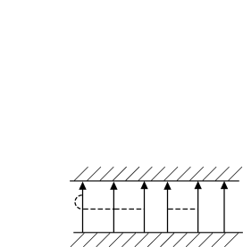
Figure 5: System of 6 nucleons interacting via pions. The cross-hatched (for emphasis) regions depict initial and final times. Solid lines are nucleons, while dashed lines are pions.

Figure (5) shows a representative case with the requisite complexity. It has $A=6$ nucleons propagating from some initial time to some final time (indicated by cross-hatching for emphasis). The process can be divided into two interacting clusters and a single noninteracting nucleon, producing $n_{c}=3$. There is a closed loop on the left-most nucleon, so that $L=1$ and $\bar{L}=4$. The very important topological parameter $n_{c}$ specifies the complexity of the interaction scenario and will determine the relative importance of $N$-nucleon forces.

A third set of variables is required to set up the counting, but will not appear in the final result:

$\diamond$ $E_{N}=$ number of interacting nucleons;

$\diamond$ $X_{N}=$ number of noninteracting nucleons;

$\diamond$ $C=$ number of interacting clusters of nucleons; (6.3)

$\diamond$ $I_{B}=$ number of boson (pion) propagators (i.e., internal lines);

$\diamond$ $I_{F}=$ number of fermion (nucleon) propagators (i.e., internal lines);

$\diamond$ $V=$ number of vertices (i.e., $\sum_{i}$).

Note that a cluster must contain at least one vertex, but can have any number (including only one) of connected nucleons. Moreover, the nucleon lines touching the cross-hatched regions are not propagators. For the case specified by Fig. (5) we have $C=2,E_{N}=5,X_{N}=1,V=6,I_{B}=4$, and $I_{F}=1$.

We have several obvious relationships between previously defined variables

$$A=X_{N}+E_{N}\,,$$

$$n_{c}=E_{N}-C\,,$$

$$V=\sum_{i}1\,.$$

Note that Eq. (6.5) does not appear to correspond precisely to Eq. (6.2). A cluster of one nucleon interacting only with itself will not contribute to $n_{c}$, and the two definitions are thus equivalent. Using the fact that two boson (pion) or fermion (nucleon) fields are needed to make each boson or fermion propagator, we have

$$\sum_{i}b_{i}=2I_{B}\,,$$

$$\sum_{i}f_{i}=2I_{F}+2E_{N}\,,$$

where by definition only interacting nucleons connect to a vertex. The number of loops in a diagram can be counted by noting that in constructing a diagram there is a four-dimensional phase-space integral associated with each propagator. Feynman diagrams conserve four-momentum at each vertex, and these constraints ($V$ of them) eliminate the integrals. This overcounts, however, since each cluster has an overall $\delta$-function (four-momentum) constraint (see the discussion below Eq. (4.1)), and there are $C$ of them. Thus, the number of loops is

$$L=I_{B}+I_{F}-V+C\,,$$

and associated with each loop is a four-(i.e., $D$-)dimensional phase-space integral $\int\frac{d^{D}p}{(2\pi)^{D}}\sim[E^{D}]$. Figure (5) has one loop, by inspection or by using Eq. (6.9). Each noninteracting nucleon contributes a three-momentum (i.e., $D-1$) $\delta$-function $\sim[E^{1-D}]$ (see Appendix A).

Finally, the momentum or energy dimensionality of any diagram can be determined by counting:
$\diamond$ phase-space factors $\sim[E^{D}]$ in loops;
$\diamond$ boson (pion) propagators ($\sim(p^{2}-m^{2}_{\pi})^{-1}\sim[E^{-2}]$);
$\diamond$ fermion propagators ($\sim(\hbox to0.0pt{$p$\hss}/-M_{N})^{-1}\sim[E^{-1}]$);
$\diamond$ derivatives in vertices ($p^{\mu}\sim[E]$);
$\diamond$ cluster $\delta$-functions $\sim[E^{-D}]$ ($C-1$ of them; one has already been removed) ;
$\diamond$ $\delta$-functions $\sim[E^{1-D}]$ for noninteracting nucleons (see above and App. A);
$\diamond$ an optional factor [in brackets below] (because it depends only on A, and not the process) that enforces the overall normalization of the wave function in momentum space (see Appendix A).
In that order we have

$$\nu=DL-2I_{B}-I_{F}+\sum_{i}d_{i}-D(C-1)-(D-1)X_{N}+[(D-1)(A-1)]\,.$$

There are 5 basic internal “variables” in Eqs. (6.7 - 6.9) (together with $C,E_{N},V$) that determine $\nu(I_{B},I_{F},L,b_{i},f_{i})$ and only those 3 relations among them; $I_{B}$ and $I_{F}$ are always eliminated. We must keep 2 of the remaining ones and choose $L$ and $f_{i}$. The other choices produce equivalent, though less useful, formulae (see Ref. [12] for a discussion of options). Eliminating $I_{B},I_{F}$ and $\sum_{i}b_{i}$ using Eqs. (6.7 - 6.9) we find

$$\nu = 1+(D-2)(n_{c}+L)+\sum_{i}\Delta_{i}-((D-1)(A-1))+[(D-1)(A-1)]$$

$$= 1+(D-2)\bar{L}+\Delta\,.\hskip 198.7425pt(6.11)$$

The constant term in square brackets cancels an identical term that arises from algebraic manipulation. Note also that the last two terms in Eq. (6.10) in effect add ($D-1$) (i.e., 3) powers (from phase-space factors) for each independent (i.e., non-center-of-mass) nuclear coordinate involved in an interaction. These powers (as we will see below in an explicit example) in effect convert from momentum to configuration space. Finally, for D = 4 we have a very simple and elegant power-counting result:

$$\nu=1+2\bar{L}+\Delta\,.$$

Except for irrelevant constant terms (depending on $A$), this agrees with Weinberg and van Kolck[11, 12].

Recall that $\bar{L}$ and $\Delta$ are separately positive semi-definite. The case $\bar{L}=\Delta=0\ (\nu=1)$ cannot occur because this would imply a single nucleon interacting without a loop; only the nucleon kinetic energy has this form and it corresponds to $\Delta=1$, as we found in Eq. (3.7). Thus, the minimum values of $\nu$ are 2, corresponding to the kinetic energy, and 3, corresponding to $NN$ forces ($n_{c}=1,L=0,\Delta=0$). See also Appendix B for another example.

We summarize this section by noting that:

$\bullet$ Powers, $\nu$, of a generic energy or momentum, $Q$, can be counted in Feynman diagrams by following the flow of momentum through each vertex.

$\bullet$ The nuclear case requires consideration of all nucleons, since all nucleons eventually interact in a bound state.

$\bullet$ The final formula for $Q^{\nu}$ is exceptionally simple, and shows that $\nu$ always increases as more complicated mechanisms are considered.

7 Electromagnetic Interactions

We can extend these results to EM interactions within strongly-interacting systems by including the “photon” as an extra boson[10]. This produces only one significant change. For EM interactions: $\Delta^{EM}_{i}\geq-1$, as noted by Rho[10]. This is compensated by a factor of $e$, the fundamental charge, which will reduce the size of amplitudes. For specificity we will illustrate the case of a single photon (virtual or otherwise) and this will allow us to discuss nuclear EM currents (either impulse-approximation or meson-exchange), $J^{\mu}_{EM}\equiv(\rho,{\bf J})$. We refer the reader to Refs. [10, 27] for more complex cases.

Separating out the (assumed) single EM vertex from Eq. (6.12), we have[10]

$$\nu_{EM}=1+2\bar{L}+\Delta_{ST}+\Delta_{EM}\,,$$

where $\Delta_{ST}$ is the sum over strong vertices ($\geq 0$) and $\Delta_{EM}$ refers to the single EM vertex $(\geq-1)$ and will differ for $\rho$ and ${\bf J}$.

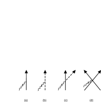
Figure 6: Lagrangian building blocks for EM interactions of pions and nucleons. Solid lines are nucleons, dashed lines are pions, and wavy lines depict photons.

Various important building blocks are shown in Fig. (6). The impulse-approximation current, $J^{\mu}_{imp}$, is shown in Fig. (6a). The relativistic form of the four-current is $\bar{N}\gamma^{\mu}N$, and involves no derivatives. We know, however, that when “odd” $\gamma$-matrices are rendered to nonrelativistic form, they are of leading order $(p/M_{N})$, while “even” ones are $\cal{O}$(1). Thus, $\Delta_{EM}=-1$ for $\rho_{imp}$ ($f=2,d=0$), while $\Delta_{EM}=0$ for ${\bf J}_{imp}$ ($f=2,d=1$). The pion EM current in Fig. (6b) has a single derivative[21] and $\Delta_{EM}=-1$, while the dominant seagull term[20, 31] shown in (6c) has $\Delta_{EM}=-1$ for $\mbox{\boldmath$J$}_{SG}$ and $\Delta_{EM}=0$ for $\rho_{SG}$. The short-range two-body three-current in (6d) has $f=4,d\geq 1$ and consequently $\Delta_{EM}\geq 1$. This suppresses the short-range contributions compared to pion-range and impulse-approximation currents. We note that the $\Delta$-isobar current (assuming that we choose not to include the $\Delta$ in our active Hilbert space) and the ($\rho\pi\gamma$) current would be (higher-order in 1/$\Lambda$) contributions[10] of the form illustrated in Fig. (6c), while the ($\omega\sigma\gamma$) current[10] would have the form in Fig. (6d).

We summarize this section by noting that:

$\bullet$ The electromagnetic current in a nucleus can be treated in a fashion similar to the energy, and this is most conveniently done by separating the EM vertex from the strong ones.
$\bullet$ Short-range MEC are suppressed compared to pion-range MEC.

8 Final Counting of Powers

Before completing the power counting, it is useful to interpret our results using a simple, familiar example. The one-pion-exchange amplitude in Fig. (1a) has the form

$$V_{\pi}(\mbox{\boldmath$q$})=-\frac{g^{2}_{A}}{f^{2}_{\pi}}\frac{\mbox{\boldmath$t$}_{1}\cdot\mbox{\boldmath$t$}_{2}\mbox{\boldmath$\sigma$}_{1}\cdot\mbox{\boldmath$q$}\mbox{\boldmath$\sigma$}_{2}\cdot\mbox{\boldmath$q$}}{\mbox{\boldmath$q$}^{2}+m^{2}_{\pi}}$$

in momentum space, where $q$ is the three-momentum transferred between nucleons “1” and “2”. In terms of power counting, $V_{\pi}({\bf q})\sim Q^{0}/f^{2}_{\pi}$. As we argued in the previous section and in Appendix A, this should be multiplied by the phase-space factor $\frac{d^{3}q}{(2\pi)^{3}}$ and the Fourier transform to configuration space completed. The phase-space factor behaves as $Q^{3}$, in agreement with Eq. (6.12) (for $n_{c}=1,L=0,\Delta=0$). Moreover, performing the momentum integrals produces a Yukawa function multiplied by the familiar factor of $1/4\pi$ (see Eq. (3.6)). The latter converts a single $f_{\pi}$ in Eq. (8.1) to a $\Lambda\ (4\pi f_{\pi}\sim\Lambda)$. Thus $V_{\pi}(r)\sim\frac{Q^{3}}{\Lambda f_{\pi}}$ as we found in Eq. (3.8). We expect that more complicated diagrams with more propagators $(n_{c}>1)$[41] will generate a factor of $1/(4\pi)^{n_{c}}$.

The interpretation of the short-range force $V_{SR}$ in Fig. (3d) is somewhat different. We again have a factor of $(1/f^{2}_{\pi})$ from Eq. (5.4) and a phase-space factor that leads to a $\delta$-function. We write the latter in the form

$$\delta^{3}({\bf r})=\frac{1}{4\pi}\frac{\delta(r)}{r^{2}}\,.$$

The factor of $1/4\pi$ is the same as before, and $\delta(r)/r^{2}\sim Q^{3}$, where $Q\sim m_{\pi}$ is the inverse correlation length that sets the scale of the correlation function. Thus, each coordinate-space $\delta$-function counts as $\sim Q^{3}/4\pi$[41]. This is actually reduced somewhat because of the repulsive nature of the short-range correlations. Nevertheless, combining everything we see that $V_{SR}$ also counts as $\frac{Q^{3}}{\Lambda f_{\pi}}$, as predicted by Eq. (6.12) with $L=\Delta=0$ and $n_{c}=1$.

Figure 7: Percentages of accrual of kinetic energy (solid line), potential energy (short dashed line), and probability (long dashed line) within an interparticle separation, $x$, for any pair of nucleons in the triton.

These concepts are illustrated nicely in Fig. (7), which shows the accrual of potential and kinetic energy in the triton. A single pair of nucleons separated by a distance $x_{12}$ is selected, and the expectation value of $\Theta(x-x_{12})\hat{O}$ is calculated, where $\hat{O}=T,V$, or 1. These values are divided by the value for $x=\infty$, and the percentage accrual is plotted. One sees that the major contribution is between 1 and 2 fm. Moreover, the short-range part of the potential energy is rather modest, starting out repulsive and then yielding to the attractive OPEP. One sees in these plots that $Q\sim m_{\pi}\sim[1.4\,{\rm fm}]^{-1}$ is a reasonable value.

We now put together all of the factors for power counting the energy in $D=4$ dimensions: $Q,f_{\pi},\Lambda$. The Lagrangian scale factors are given in Eq. (5.4). We also expect a factor of $(4\pi)^{-2L}$ from loops (see Appendix B for a discussion of this and a possible counterexample) and $(4\pi)^{-n_{c}}$ from configuration-space propagators (see above). This gives our final result for $\langle\hat{E}\rangle$, where $\hat{E}$ is any irreducible contribution to the energy, in terms of the different scales:

$$\langle\hat{E}\rangle\sim\frac{Q^{1+2(n_{c}+L)+\Delta}f^{2V-f-b}_{\pi}}{\Lambda^{\Delta}(4\pi)^{2L}(4\pi)^{n_{c}}}\\$$

$$=Q\left(\frac{Q}{f_{\pi}}\right)^{n_{c}}\left(\frac{Q}{\Lambda}\right)^{2L+n_{c}+\Delta},$$

using $f+b\equiv\sum_{i}(b_{i}+f_{i})=2V+2(n_{c}+L)$ obtained from Eqs. (6.5 - 6.9), and $\Lambda\sim 4\pi f_{\pi}$. When counting for other observables (viz., the T-matrix), the number of external bosons explicitly enters the equations[11], and this changes the factors that set the energy scales. Our formula reproduces all of the previous results obtained using less sophisticated techniques. Specific applications are relegated to the next section.

We summarize this section by noting that:

$\bullet$ Various nuclear energies behave as $Q^{\nu}/\Lambda^{\nu-n_{c}-1}f^{n_{c}}_{\pi}$, with more complicated mechanisms having larger values of $\nu$ and $n_{c}$.
$\bullet$ This formula includes phase-space factors required for conversion to configuration space, and incorporates momentum sharing between the nucleons.

9 Results and Discussion

The most important aspect of this work concerns the relative sizes of $N$-nucleon forces. The leading-order force connecting $N$ nucleons will have $L=0,\Delta=0$, and $n_{c}=N-1$, corresponding to the simplest possible calculation (all others with $L>0,\,\Delta>0$ will be smaller). This produces

$$\langle V_{NNF}\rangle\sim\frac{Q^{2N-1}}{(f_{\pi}\Lambda)^{N-1}}\sim\frac{Q^{N}}{\Lambda^{N-1}}\,,$$

where we have used $Q\sim f_{\pi}$ in order to make the final estimate. We can also use the additional results of Ref. [16], who found that

$$\langle V_{NN}\rangle\;\sim 20\,{\rm MeV/pair}\,,$$

$$\langle V_{3NF}\rangle\;\sim 1\,{\rm MeV/triplet}\,,$$

$$\langle V_{4NF}\rangle\;\;\mathrel{\raise 3.0pt\hbox to8.0pt{\raise-6.0pt\hbox{$\sim$}\hss{$<$}}}.1\,{\rm MeV/quartet}\,.$$

This geometric decrease of the net contribution of many-body forces is consistent with Eq. (9.1) and is one of the most important results of Ref. [16], since it confirms the role of chiral symmetry in suppressing many-body forces in nuclei.

Resurrecting the old formalism of Ref. [20] (applied to pions interacting in a nucleus) also provides some insight into the structure of Eq. (8.3). That work was predicated upon performing a nonrelativistic expansion of operators using a Foldy-Wouthuysen procedure, constructing nuclear operators using the superposition principle, and then performing time-dependent perturbation theory. The nucleons in such a formalism propagate only forward in time, although mesons go forward or backward. Because the operators refer to the entire nucleus (e.g., $J=\sum^{A}_{i=1}J_{i}$ for some impulse-approximation vertex, $J_{i}$), so do the propagators. One simply constructs $(E-H)^{-1}\sim[E^{-1}]$ in terms of the nuclear Hamiltonian, $H$ (details can be found in Refs. [19, 20]). Thus, power counting should be exactly the same as we have already derived, although it will be necessary to redefine the variables. This configuration-space formalism automatically incorporates phase-space factors.

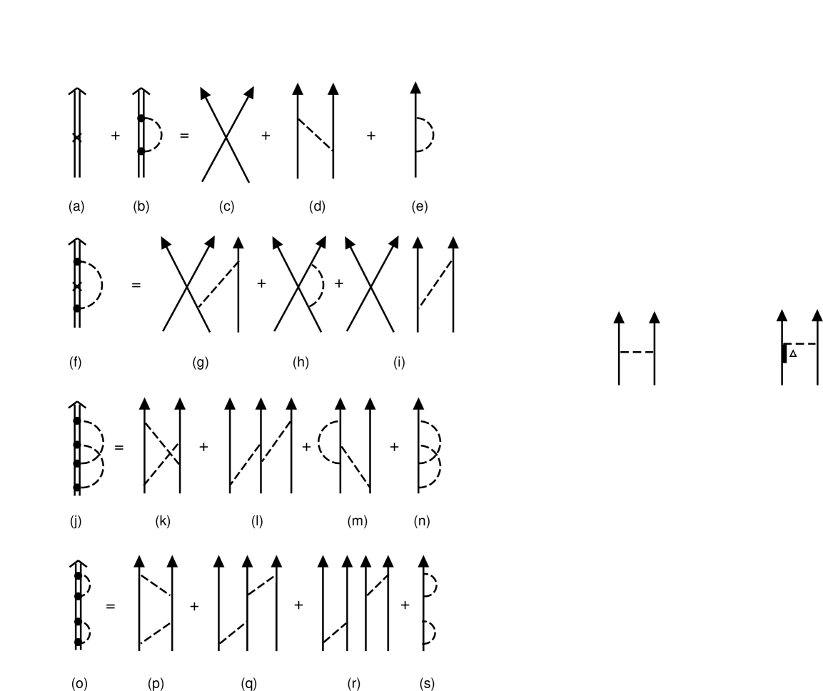
Figure 8: Contributions to the nuclear energy from “nucleus” diagrams on the left, broken down into the usual “nucleon” diagrams on the right. Single solid lines are nucleons, double solid lines represent a nucleus, dashed lines are pions, while a cross depicts a short-range interaction in the nucleus approach.

Typical diagrams are shown in Figure (8), with diagrams from Ref. [20] on the left expanded as a set of diagrams on the right, where noninteracting nucleons are suppressed for simplicity. Although the “nucleus” diagrams subsume many distinct mechanisms when expanded into “nucleon” diagrams, all of the latter share the same topology specified by the former, and this we wish to explore. The cross represents the short-range interaction, while the double lines represent a nucleus propagator, or a nucleus wave function, and the large dots represent the pion-nucleus vertex, $J$. Not all diagrams are shown.

Figure (8a) for a nucleus is equivalent to Fig. (8c). Figure (8b) can be expanded into Figs. (8d) and (8e). Because the vertices in the “nucleus” formalism contain all nucleons, expanding second-order perturbation theory leads to both pion exchanges (8d) and loops (8e) (only one of the loops is shown, and this is calculated in Appendix B). Moreover, we see that all possible orderings are included, and that the “loop-like” appearance of the nucleus diagrams results from the forward-propagating nucleus. We count these diagrams as $\nu=1+2\bar{L}+\bar{\Delta}$, where $\bar{L}$ is the number of “nucleus loops”. If we wish to power-count for these “nucleus” diagrams, we must recall that increasing the number of connected nucleons by 1 increases $\nu$ by 2. Thus, we must count the short-range interaction as $\bar{\Delta}=2$. This is a simple rearrangement of our original form, moving part of $n_{c}$ into $\Delta$. Note that if one end of a propagator in a nucleon loop (e.g., in Fig. (8e)) is detached and reattached to another nucleon (as in Fig. (8d)), we lower $L$ by 1 and increase $n_{c}$ by 1, keeping $\bar{L}\equiv n_{c}+L$ fixed, and this is why powers of $Q$ depend only on the combination $(n_{c}+L)=\bar{L}$. Both types count the same and are subsumed in nucleus diagrams (e.g., Fig (8b)). Because different integrals generate different factors of $(1/4\pi)$, the counting of $\Lambda$ factors (which leads to Eq. (8.3); see Appendix B) can be different. In this example, however, both mechanisms behave as $Q^{3}/\Lambda f_{\pi}$ (in leading order).

Figure (8f) subsumes the graphs of Figs. (8g) - (8i), all of which have $\nu=5$, but differing values of $L,n_{c},C$, etc. Note that this set of diagrams includes three-nucleon forces, vertex corrections to an $NN$ force (only one of which is illustrated in Fig. (8h)) and a “recoil” graph (with $C=2$) in Fig. (8i) (which is a special problem treated later). The graphs of Fig. (8j) comprise those of Figs. (8k) - (8n) plus several others that are disconnected $(C=2)$, and all have $\nu=5$.

Our final example treats the “infrared” singularities discussed in Section 3. A typical case is Fig. (8o), which subsumes Figs. (8p) - (8s). Nominally the graph has $\bar{L}=2$ and thus $\nu=5$. However, if any of the previous graphs are sliced in two by a horizontal line, the pion lines are cut, implying a minimum energy at that time of $Q\sim E_{\pi}$ in those propagators. This also holds for Fig. (8o) as long as the horizontal line intersects a pion propagator. However, a very different result holds when only the nucleus propagator ($\sim\frac{1}{E-H}\sim 1/(Q^{2}/M_{N})\sim\frac{M_{N}}{Q^{2}}$, rather than $1/Q$) is intersected. In that case the energy in the propagator is much smaller. These diagrams are therefore enhanced, as we discussed earlier, when the Schrödinger equation is solved. For this reason, one chooses to define the Schrödinger Hamiltonian in terms of irreducible operators, which are then incorporated into the Schrödinger equation. The “reducible” diagrams not only count differently (we must add a factor of $\Lambda/Q$ for each infrared propagator, including those in loops, and adjust factors of $4\pi$ [see App. C]), but they also contribute to the “recoil graph” problem.

That problem arises because graphs of the type shown in Fig. (1b) depend on the energy of the nucleus $(E_{0})$ and this is contained in nuclear propagators: $(E_{\pi}+H-E_{0})^{-1}$. Because $H$ and $E_{0}\sim Q^{2}/\Lambda$ and $E_{\pi}\sim Q$, it is conventional to expand the propagator in powers of $(E_{0}-H)/E_{\pi}\sim\frac{Q}{\Lambda}$. Although $(E_{0}-H)$ acting on an initial or final wave function vanishes, it can also kill the propagator in the middle of Fig. (8o), leading to an irreducible operator. Thus the special feature of reducible diagrams leads to a “freedom” in the form of reducible operators that we choose to incorporate into our theoretical structure, depending on where we place parts of various operators. Experience has shown that disconnected, but overlapping graphs, of the type shown in Fig. (8i) can be removed (if desired) using a rearrangement, as can the leading order of extended overlapping graphs of the type shown in (8g) and (8l). This rather technical subject can be reviewed in Refs. [19, 20, 25]. The practitioner should beware of any graph where a nucleon propagator is not required by kinematics to carry an energy $\sim E_{\pi}$ (as in (8g) or (8l)) or graphs that are disconnected (as in (8i)).

As an example of how rearrangement affects the power counting, it has been shown that the nominal value of $\nu=5$ (obtained from Eq. (8.3)) can be changed to $\nu=6$ (as we already saw in Eq. (3.10)) for the 3NF type in Fig. (8l), and this also holds for the process in Fig. (8g). The short-range 3NF resulting from the interaction of 3 nucleons (Fig. (3e)) has $n_{c}=2,\Delta=1$, and hence $\nu=6$. Thus, the leading 3NF can be manipulated into $\nu=6$ (rather than 5) by a suitable definition of the nuclear Hamiltonian. Note that there is a factor of $1/\Lambda$ associated with the additional factor of $Q$. These different choices are neither right nor wrong; they are a theorist’s choice. One must simply be consistent.

Figure 9: Meson-exchange currents of various types. Solid lines depict nucleons, dashed lines show pions, while wavy lines illustrate the EM interaction.

Our final examples treat a few of the meson-exchange currents in EM interactions. Using the rules we developed earlier, the power counting for the four $(n_{c}=1)$ graphs in Fig. (9) for $\vec{J}_{MEC}$ gives 2, 2, 4, 4, respectively, assuming that the $\Delta$-isobar is treated as a heavy particle (showing that $\Delta_{EM}\geq 1$ for Fig. (9d) is left as an exercise[10]). One can show[10, 20] that graphs (a) and (b) contain a factor of $(4\pi f^{2}_{\pi})^{-1}$, [(c) and (d) have an additional factor of $\Lambda^{-2}$], so that these leading-order MEC behave as $Q^{2}/f_{\pi}\Lambda\sim Q/\Lambda$, and should be comparable to the impulse-approximation result $\sim\mbox{\boldmath$p$}/M_{N}\sim Q/\Lambda$. This precisely conforms to the old “rules of scale”. The isobar and heavy-meson MEC are suppressed by an additional factor of $(Q/\Lambda)^{2}$. Moreover, this counting is valid on both sides of the current-continuity equation

$$\mbox{\boldmath$\nabla$}\cdot{\bf J}({\bf x})=-i[H,\rho({\bf x})]\,,$$

using Eq. (9.1).

The nonrelativistic charge operator is ${\cal{O}}(1)$, and impulse-approximation relativistic corrections are ${\cal{O}}(Q^{2}/\Lambda^{2})$. The pion-exchange currents (see Appendix A of Ref. [19]) are ${\cal{O}}(Q^{3}/4\pi f^{2}_{\pi}M_{N}\sim Q^{3}/f_{\pi}\Lambda^{2}\sim Q^{2}/\Lambda^{2})$, consistent with $\Delta_{EM}=0$ for the seagull charge operator. Note that $Q^{2}/\Lambda^{2}$ is really the same as $(v/c)^{2}$, and this also conforms to the old rules of scale[18, 20].

Additional special cases are worked out in the literature[11, 12, 27, 30, 31, 40].

We summarize this section by noting that:

$\bullet$ $N$-nucleon forces scale at least as fast as $(Q/\Lambda)^{N-1}$, implying that two-nucleon forces are stronger than three-nucleon forces are stronger than four-nucleon forces …  .

$\bullet$ Results of recent few-nucleon calculations are consistent with this result, which makes nuclear physics tractable.

$\bullet$ The topology of “nucleus” (as opposed to “nucleon”) diagrams accounts for important aspects of the latter.

$\bullet$ Infrared singularities (reducible diagrams) enhance the Schrödinger perturbation series.

$\bullet$ Different treatments of “recoil-graphs” (resulting from IR singularities) can lead to changes in power-counting rules (always making terms weaker than naive power-counting predictions).

$\bullet$ Power counting for electromagnetic processes is consistent with the current-continuity equation.

$\bullet$ Heavy-meson MEC are suppressed relative to one-pion-exchange terms.

10 Conclusions

We have developed systematically the power-counting rules of Weinberg, and have added additional expository material and numerous examples. Chiral symmetry provides order, and the QCD scale $\Lambda$ plays a deterministic role. We have shown that the nuclear kinetic and potential energies (“intrinsic”/pair) scale roughly as $Q^{2}/\Lambda$, consistent with weakly-bound systems. $N$-nucleon forces are suppressed as $N$ increases. Increasingly complex contributions to the force progressively weaken. Short-range meson-exchange currents are weaker than pion-range currents, which are comparable to impulse-approximation currents. Large strong-interaction coupling constants of heavy-mesons to nucleons result from the mismatch of the scales $f_{\pi}$ and $\Lambda$.

All of these results have been stated before in one form or another using a variety of arguments or empirical observations, but their totality rests on power counting. In the words of S. Weinberg[44],

“The chiral Lagrangian approach turns out to justify assumptions (such as assuming the dominance of two-body interactions) that have been used for many years by nuclear physicists …”

11 Acknowledgements

This work was performed under the auspices of the United States Department of Energy. The author would like to thank Bira van Kolck for providing valuable insights into how strong-interaction physics works and for advice on the manuscript. He would also like to thank E. Tomusiak, S. Coon, and P. Bedaque for similar advice.

12 Appendix A – Momentum Space to Configuration Space

We have relegated a tedious but instructive part of our derivation to this Appendix. We have chosen the option of power counting in configuration space. A straightforward power-counting derivation in momentum space does not involve the last two terms in Eq. (6.10), which arise from the conversion to configuration space. These terms are vital, since they reset the baseline (for fixed $A$) against which we determine the importance of various operators. As we will see below, it amounts simply to incorporating phase-space factors for each independent degree of freedom in a nucleus. In $D-1$ space dimensions, there are $(D-1)(A-1)$ independent internal degrees of freedom, plus $D-1$ that specify the motion of the nuclear center-of-mass (CM) and don’t play any role in our discussion.

We wish to calculate $\langle\Psi_{f}|\hat{O}|\Psi_{i}\rangle$ in both momentum and configuration spaces (for $D=4$). We write

$$\Psi_{f,i}(\{{\bf r}^{\prime}_{i}\})=\int\frac{\Pi_{i}\,(d^{3}p^{\prime}_{i}\,e^{i{\bf p}^{\prime}_{i}\cdot{\bf r}^{\prime}_{i}})}{(2\pi)^{3(A-1)}}\;\;\delta^{3}\left(\sum_{k}{\bf p}^{\prime}_{k}\right)\Psi_{f,i}(\{{\bf p}^{\prime}_{j}\})\,,$$

where our notation “$\{\}$” emphasizes that the wave function depends on the set of internal coordinates $\{{\bf r}^{\prime}_{j}\}=({\bf r}^{\prime}_{1},{\bf r}^{\prime}_{2},\ldots)$ or momenta $\{{\bf p}^{\prime}_{j}\}$, and we have removed the CM coordinates ($\sum_{j}{\bf r}^{\prime}_{j}\equiv 0$ and $\sum_{j}{\bf p}^{\prime}_{j}\equiv 0$). It is a convenience to treat the coordinates ${\bf r}^{\prime}_{j}$ as independent and use a $\delta$-function as the constraint. As a check, we evaluate the normalization integral:

$$\langle\Psi_{f}|\Psi_{i}\rangle\equiv\int\Pi_{i}\,(d^{3}r^{\prime}_{i})\,\delta^{3}\left(\sum_{k}{\bf r}^{\prime}_{k}/A\right)\Psi^{\dagger}_{f}\left(\{{\bf r}^{\prime}_{j}\}\right)\Psi_{i}(\{{\bf r}^{\prime}_{j}\})\\$$

$$=\int\frac{\Pi_{i}(d^{3}p^{\prime}_{i})}{(2\pi)^{3(A-1)}}\delta^{3}\left(\sum_{k}{\bf p}^{\prime}_{k}\right)\Psi^{\dagger}_{f}(\{{\bf p}^{\prime}_{j}\})\;\Psi_{i}(\{{\bf p}^{\prime}_{j}\})=1\;.$$

The factor of $A$ in the ${\bf r}^{\prime}_{k}$ $\delta$-function is conventional. Thus, in order to obtain the expectation value of an operator in configuration space, $\langle\hat{O}\rangle$, we need to: (1) look at the operator in momentum space and (2) multiply by the requisite number of independent phase-space factors as given in Eq. (A2). This adds $[(D-1)(A-1)]$ momentum factors to $\nu$ (accounting for the last term in Eq. (6.10)) and resets the baseline for each diagram or process. Note that if we evaluate $\langle\Psi_{f}|T|\Psi_{i}\rangle$, where $T$ is the kinetic energy, we simply insert $\sum_{j}{\bf p}^{\prime\,2}_{j}/2\,M_{N}$ between the wave functions in the second form of Eq. (A2), which is an obvious result.

If we take the expectation value of a two-body operator, $V_{ij}(r_{ij})$, then a somewhat different form results

$$\langle V_{12}\rangle=\int\frac{\Pi_{i}(d^{3}q^{\prime}_{i})}{(2\pi)^{3(A-1)}}\delta^{3}\left(\sum_{k}{\bf q}^{\prime}_{k}\right)\int\frac{d^{3}p}{(2\pi)^{3}}\\$$

$$\Psi^{\dagger}_{f}({\bf p}+{\bf q}^{\prime}_{1},-{\bf p}+{\bf q}^{\prime}_{2},\ldots)\,V_{12}({\bf p})\,\Psi_{i}({\bf q}^{\prime}_{1},{\bf q}^{\prime}_{2},\ldots)\,.$$

In addition to the conventional offset $((D-1)(A-1))$, the two-body potential inherits a phase-space factor: $\frac{d^{3}p}{(2\pi)^{3}}$. This is already included in Eq. (6.11) because of momentum sharing. The phase-space factors above serve to kill all the $\delta$-functions from non-interacting nucleons, leaving phase-space factors (in effect) only for interacting nucleons. This accounts for the $\frac{d^{3}p}{(2\pi)^{3}}$ in Eq. (A3). Thus by including momentum sharing with “non-interacting” nucleons and a full set of phase-space factors, we have reset the baseline so that our power counting works in the same fashion for any nucleus and any operator. Our final results do not depend on $A$. Naive power counting of the potential in momentum space produces $Q^{0}$ for OPEP; the phase space factor makes this $Q^{3}$, as we derived earlier $(n_{c}=1,\Delta=L=0\rightarrow\nu=3)$. Three-nucleon operators pick up an additional phase-space factor, and so on. This completes the interpretation of various factors in the power counting.

We summarize this appendix by noting that:

$\bullet$ Inclusion of Fourier-transform phase-space factors resets the baseline for all diagrams.

$\bullet$ This generates a diagram-independent offset $[(D-1)(A-1)]$ that makes our final power-counting formula independent of $A$.

13 Appendix B

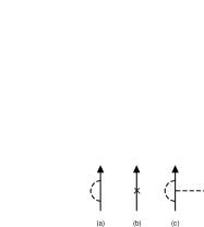
Figure 10: A single nucleon interacting with pions. Solid lines are nucleons, dashed lines are pions, and the cross depicts a mass counter term.

A wide variety of concepts can be illustrated by working out a simple example in toto. Figure (10a) illustrates the self-energy of a nucleon arising from pionic vacuum fluctuations. We perform a nonrelativistic calculation of the S-matrix, noting that the nucleon self energy $\sum_{N}$ is traditionally defined by $S=-i\Sigma_{N}\;[(2\pi)^{4}\delta^{4}(P_{f}-P_{i})]$:

$$\Sigma_{N}=i\left(\frac{g_{A}}{f_{\pi}}\right)^{2}\int\frac{d^{4}k}{(2\pi)^{4}}\;\;\frac{(\mbox{\boldmath$\sigma$}\cdot\mbox{\boldmath$k$})^{2}\,{\bf t}^{2}}{(k^{2}_{0}-E^{2}_{\pi}+i\epsilon)(-k_{0}+E-\frac{({\bf p}+{\bf k})^{2}}{2M_{N}}+i\epsilon)}\,,$$

using the Feynman rules: $\frac{g_{A}}{f_{\pi}}t^{\alpha}\mbox{\boldmath$\sigma$}\cdot{\bf k}$ for creating a pion with isospin component $\alpha$, momentum $k^{\mu}$, and spin $\sigma$, which corresponds to $\Delta=0$. We have included (for now) the complete nucleon propagator (energy $E={\bf p}^{2}/2\,M_{N}$, momentum ${\bf p}$), and have defined the pion energy by $E^{2}_{\pi}={\bf k}^{2}+m^{2}_{\pi}$. Using $(\mbox{\boldmath$\sigma$}\cdot{\bf k})^{2}={\bf k}^{2},{\bf t}^{2}=3/4$, and noting that there is a single pole in the lower $k_{0}$-plane we obtain

$$\Sigma_{N}=-\frac{3}{8}\left(\frac{g_{A}}{f_{\pi}}\right)^{2}\int\frac{d^{3}k}{(2\pi)^{3}}\frac{\hskip 10.84006pt{\bf k}^{2}}{E_{\pi}\left(E_{\pi}+\frac{({\bf p}+{\bf k})^{2}-{\bf p}^{2}}{2M_{N}}\right)}\,.$$

To leading order in $1/M_{N}$, we can ignore the kinetic-energy terms $\sim 1/M_{N}$. We also note that the pion energy sets the scale in both of the propagators. Much of the power counting that we did earlier depends explicitly on this fact. Thus to leading order in $(1/M_{N})$, we obtain the cubically divergent result

$$\Sigma_{N}=-\frac{3}{8}\left(\frac{g_{A}}{f_{\pi}}\right)^{2}\int\frac{d^{3}k}{(2\pi)^{3}}\;\;\frac{{\bf k}^{2}}{({\bf k}^{2}+m^{2}_{\pi})}\,.$$

Interpreting this result requires further work. First, we must regularize the integral and render it finite. Then we must renormalize. The method of choice is dimensional regularization. We convert the 3-dimensional integral to $n$ “space” dimensions ($\int\frac{d^{n}k}{(2\pi)^{n}}$, with $n$ not necessarily an integer), and evaluate it for some $n$ where $\Sigma_{N}$ is finite, renormalize the result, and analytically continue this finite value to $n=3$. The angular integrals plus factors of $2\pi$ give[45]

$$\int\frac{d\Omega_{n}}{(2\pi)^{n}}=\frac{2}{\Gamma(n/2)(4\pi)^{n/2}}\,,$$

and we see the origin of factors of $4\pi$. The remaining integral is[46]

$$\int^{\infty}_{0}\frac{dk\;k^{n+1}}{(k^{2}+m^{2}_{\pi})}=-\frac{m^{n}_{\pi}}{2}\cdot\frac{\pi}{\sin(\frac{n\pi}{2})}\,.$$

For $n<0$ these integrals are finite, and their extension to $n=3$ (or any odd dimension) is also finite. Combining Eqs. (B4) and (B5) for $n=3$ produces $m^{3}_{\pi}/4\pi$.

At first sight this is a very strange procedure, and the reader is referred to Ref. [15] for more expert justification. We note that by adding and subtracting $m^{2}_{\pi}$ in the numerator of the integrand in Eq. (B3) we obtain $\int\frac{d^{3}k}{(2\pi)^{3}}$, which has no length or energy scale and therefore has no obvious physics associated with it (so we drop it), plus another term. This process can be repeated, producing another scaleless integrand ($-m^{2}_{\pi}\int\frac{d^{3}k}{(2\pi)^{3}k^{2}}$) plus $\left[\frac{m^{3}_{\pi}}{4\pi}\right]$, the last part of which we obtained previously using Eqs. (B4) and (B5). Thus, we finally obtain a well-known result[14]

$$\Sigma_{N}=-\frac{3g^{2}_{A}m^{3}_{\pi}}{32\pi f^{2}_{\pi}}=-\frac{3g^{2}_{A}m^{3}_{\pi}}{8f_{\pi}(4\pi f_{\pi})}\sim\frac{m^{3}_{\pi}}{f_{\pi}\Lambda}\,.$$

Manipulations of the type used here to interpret our results should never be performed when they introduce singularities at $k=0$ (ours were finite there).

What is the interpretation of our procedure, and why did we keep a single term and argue away the rest? Figure (10b) also occurs as a part of $\Sigma_{N}$. This term is simply $M^{0}_{N}$, the “bare” nucleon rest mass. The divergent (but scaleless) integrals can be viewed as contributions to $M^{0}_{N}$. Since we did not know $M^{0}_{N}$ anyway, adding terms to it does not introduce a complication. The same is true for $\Sigma_{N}$ above, but its properties are special. Our original methodology was to divide the physics into soft (long-range) and hard (short-range) parts. The scaleless terms are hard (divergent), but $\Sigma_{N}$ is soft. It is proportional to $m^{3}_{\pi}\sim Q^{3}$ in accord with our counting rules $(L=1,n_{c}=0,\Delta=0)$ and is nonanalytic in $m^{2}_{\pi}$. That is, it has the form $\sqrt{m^{6}_{\pi}}=m^{2}_{\pi}\sqrt{m^{2}_{\pi}}$. Because pion masses must appear in the Lagrangian as powers of $m^{2}_{\pi}$, the square root is special. Nonanalytic terms are usually logarithms, but not always. It is a common practice[27, 34] to separate out all nonanalytic (soft) terms and lump all analytic terms (even finite ones) with the so-called “counter” terms (hard terms such as $M^{0}_{N}$). Nevertheless, because the nonanalytic terms have a special form (and are often large), we make the separation: $M_{N}\equiv M^{0}_{N}+\Sigma_{N}$. Note that $M_{N}\sim\Lambda$, but $\Sigma_{N}\sim m^{3}_{\pi}/f_{\pi}\Lambda\sim m^{2}_{\pi}/\Lambda$ and is significantly smaller, as we expect on the basis of power counting ($L=1,n_{c}=0,\Delta=0\rightarrow\nu=3$).

Finally, we note that a single factor of $1/4\pi$ arose in Eq. (B6). This is somewhat unusual, as normally loop integrals generate $1/(4\pi)^{2}$ or something similar. A single $(1/4\pi)$ arises in nonrelativistic cases corresponding to odd-dimensional (for $n=3$) integrals, such as Eq. (B3). In each case the nonanalytic term is an odd polynomial. In the usual case such as Fig. (10c) one obtains $1/(4\pi)^{2}$ and a logarithm. A useful and instructive exercise is to calculate Fig. (10a) covariantly. One finds that, indeed, all terms generate an explicit factor of $1/(4\pi)^{2}$. If one expands that result for small $m_{\pi}/M_{N}$, one finds

$$\Sigma^{Rel}_{N}=\frac{a\,M^{3}_{N}+b\,M_{N}m^{2}_{\pi}+c\,m^{4}_{\pi}/M_{N}}{(4\pi f_{\pi})^{2}}+\Sigma_{N}-\frac{3g^{2}_{A}m^{4}_{\pi}\log(m_{\pi}/M_{N})}{2M_{N}(4\pi f_{\pi})^{2}}+\cdots\,,$$

where $a$, $b$, and $c$ are dimensionless, and $a$ and $b$ are divergent. The $a-c$ terms are analytic functions (polynomials) of $m^{2}_{\pi}$ and can be incorporated directly into $M^{0}_{N}$, as we discussed above. The two scaleless integrals that we found above contribute to a and b, respectively. The logarithmic term is unique in the expansion.

In performing the expansion in Eq. (B7) that produces $\Sigma_{N}$ (Eq. (B6)), a factor of $\pi/2$ is generated, leading to a single residual factor of $\pi$ in the denominator of Eq. (B6). The logarithmic term has a dimensionless coefficient of $3g^{2}_{A}/2\sim 2.4$ and a factor of $1/(4\pi)^{2}$, which was assumed in our derivation of Eq. (8.3) that leads to $\Sigma_{N}\sim Q^{3}/\Lambda^{2}$. If we force Eq. (B6) into this form a very large dimensionless coefficient of $-3\pi g^{2}_{A}/2\sim-7.5$ results. Sometimes this happens.

Our nonrelativistic calculation reproduced the leading-order nonanalytic part of the covariant calculation (and was much easier). Although the analytic parts of the two calculations are different, they are not required to be the same and this cannot affect the final results, since we do not a priori know $M^{0}_{N}$.

We summarize this appendix with the following observations:

$\bullet$ Sensible nonrelativistic field-theory calculations are possible.

$\bullet$ Dimensional regularization is an easy way to make integrals finite.

$\bullet$ Loops can be rendered into analytic (typically “hard”) parts that are incorporated into coupling constants and nonanalytic (“soft”) parts, which are kept separate.

$\bullet$ Power counting works for loops.

$\bullet$ The pion mass controls the scale of loop propagators.

$\bullet$ Factors of $1/(4\pi)^{2}$ (and occasionally $(1/4\pi)$) arise from loops.

$\bullet$ Since $\Lambda\sim 4\pi f_{\pi}$ and $Q\sim f_{\pi}$, counting powers of $Q/\Lambda$ is not very different from counting powers of ($1/4\pi$).

14 Appendix C: Zero-Range Model

Another excellent example is the zero-range force[11]. We write the Lagrangian for two identical nonrelativistic nucleons[47] interacting via a zero-range force as

$${\cal{L}}=N^{\dagger}({\bf x},t)(i\frac{\partial}{\partial t}+\frac{\mbox{\boldmath$\nabla$}^{2}}{2M_{N}})N({\bf x},t)-\lambda(N^{\dagger}({\bf x},t)N({\bf x},t))^{2}\,.$$

The form of the scattering amplitude generated by this Lagrangian is a series of loop diagrams, each order (in $\lambda$) being a product of loops involving the two nucleons. Performing the $k_{0}$ integral (part of the $d^{4}k/(2\pi)^{4}$ phase-space factor in each loop) leads directly to the Schrödinger equation corresponding to an energy $E=k^{2}/2\mu$ and the nuclear (CM) Hamiltonian:${\bf p}^{2}/2\mu+2\lambda\delta^{3}(\mbox{\boldmath$r$})$, where $r$ is the separation of the nucleons and $\mu$ is the reduced mass. We have combined the kinetic energies of the two nucleons so that $M_{N}$ is twice $\mu$; note the combinatorial factor (of two) in front of the potential. That equation can be written in the form[47] (note that $G_{0}(r)=-\frac{2\mu}{4\pi}\frac{e^{ikr}}{r}$):

$$\Psi({\bf r})=\Psi_{0}({\bf r})+\int d^{3}r^{\prime}\,G_{0}({\bf r}-{\bf r}^{\prime})\,V({\bf r}^{\prime})\,\Psi({\bf r}^{\prime})\,,$$

where $V({\bf r}^{\prime})$ is the ($\delta$-function) potential, $\Psi_{0}({\bf r})$ is a plane wave, and $G_{0}({\bf z})$ is the Green’s function: $(E-H+i\epsilon)^{-1}$. Performing the integral, we obtain

$$\Psi({\bf r})=\Psi_{0}({\bf r})+2\lambda\,G_{0}({\bf r})\,\Psi(0)\,,$$

the “zero-range” solution; setting $r$ to 0 produces an algebraic equation

$$\Psi(0)=\frac{\Psi_{0}(0)}{1-2\lambda\,G_{0}(0)}\,,$$

from which we obtain the T-matrix[47] (unitarity implies $Im(T)=-2\mu k|T|^{2}/4\pi$):

$$T=\frac{2\lambda}{1-2\lambda\,G_{0}(0)}\,.$$

The Green’s function at the origin is (of course) linearly divergent, but we can apply the regularization techniques of Appendix B:

$$G_{0}(0)=2\mu\int\frac{d^{3}p}{(2\pi)^{3}}\frac{1}{(k^{2}-p^{2}+i\epsilon)}$$

$$\rightarrow\frac{-k\,\mu\,i}{2\pi}\,,$$

where again the “$n$-dimensional” integral is finite (and is left as an exercise, being only slightly different from Eq. (B5)). This produces

$$T=\frac{2\lambda}{1+\frac{k\,\mu\,\lambda i}{\pi}}\,,$$

which corresponds to a scattering length, $a=\mu\,\lambda/\pi$, an S-matrix,
$S=(1-i\,ka)/(1+i\,ka)$, and an effective-range function (the inverse of the K-matrix), $k\,\cot(\delta)=-1/a$.

We know that poles in the T-matrix indicate special states. A single pole always exists in this model for

$$k=\frac{\pi i}{\mu\lambda}\equiv i\kappa\,,$$

and

$$E=\frac{-\kappa^{2}}{2\mu}\sim 1/\lambda^{2}\,.$$

This corresponds to a bound state if $\lambda>0$ and to a “virtual” state if $\lambda<0$.

This is a most peculiar result, since we started with a potential that is repulsive if $\lambda>0$, and as $\lambda\rightarrow 0$ the bound state gets deeper! One must remember that the original problem (interpreted as a quantum mechanics problem) has no solution at all. We have generated a solution by changing the problem, redefining $G_{0}(0)$ and making it finite, and the peculiar properties of (C8) are a reflection of the original (insoluble) problem. This redefinition is equivalent to defining how loops (vacuum fluctuations) contribute. Thus, $\lambda$ is really the renormalized coupling constant (of arbitrary sign after renormalization), and not the “bare” one in Eq. (C1). How one might interpret and treat these peculiarities is discussed in Ref. [48].

What about $\lambda\rightarrow 0$  ? This won’t happen in general, since applying Eq. (5.4) leads to the equivalence

$$\lambda\equiv\frac{c_{\lambda}}{f^{2}_{\pi}}\,,$$

with $|c_{\lambda}|\sim 1$, and using $2\mu=M_{N}\sim\Lambda\sim 4\pi f_{\pi}$, we find

$$\kappa=\frac{(4\pi f_{\pi})f_{\pi}}{(2\mu)2c_{\lambda}}\sim\frac{f_{\pi}}{2c_{\lambda}}\sim Q\,,$$

as well as $E\sim\frac{-f^{2}_{\pi}}{4c^{2}_{\lambda}\Lambda}$ and $a\sim 2c_{\lambda}/f_{\pi}$. A bound state with binding energy $\sim$ 2.5 MeV and a corresponding scattering length $\sim 4.3$ fm is generated for $c_{\lambda}\sim 1$. The case $c_{\lambda}\sim-1$ produces a scattering length $\sim-4.3$ fm. We note that an anomalously small $c_{\lambda}$ is very improbable.

The unitarity of the T-matrix in lowest-order PT relates the first- and second-order amplitudes with a single factor of $1/(4\pi)$. The (second-order PT) loop integral must therefore be of the type that generates a single factor, rather than the usual $1/(4\pi)^{2}$.

References

- [1] H. Georgi, Weak Interactions and Modern Particle Theory, (Benjamin, Menlo Park, 1984).
- [2] J. F. Donoghue, E. Golowich, and B. R. Holstein, Dynamics of the Standard Model, (Cambridge University Press, Cambridge, 1992).
- [3] J. L. Friar, G. L. Payne, V. G. J. Stoks, and J. J. de Swart, Phys. Lett. B 311, 4 (1993); R. B. Wiringa, V. G. J. Stoks, and R. Schiavilla, Phys. Rev. C 51, 38 (1995).
- [4] W. Glöckle et al., in Few-Body Problems in Physics ’95, ed. by R. Guardiola, Few-Body Systems Suppl. 8, 471 (1995).
- [5] J. L. Friar, Czech. J. Phys. 43, 259 (1993); J. L. Friar, in Proceedings of the XIV International Conference on Few-Body Problems in Physics, ed. by F. Gross, AIP Conference Proceedings 334, 323 (1995); J. L. Friar, in Few-Body Problems in Physics ’95, ed. by R. Guardiola, Few-Body Systems Suppl. 8, 471 (1995).
- [6] D. K. Campbell, in Nuclear Physics with Heavy Ions and Mesons, ed. by R. Balian, M. Rho, and G. Ripka (North-Holland, Amsterdam, 1978), p. 551. This is a very readable article about chiral symmetry.
- [7] A. Manohar and H. Georgi, Nucl. Phys. B234, 189 (1984).
- [8] S. Weinberg, Physica A 96, 327 (1979); S. Weinberg, in A Festschrift for I. I. Rabi, Transactions of the N. Y. Academy of Sciences 38, 185 (1977).
- [9] J. L. Friar, B. F. Gibson, and G. L. Payne, Phys. Rev. C 30, 1084 (1984).
- [10] M. Rho, Phys. Rev. Lett. 66, 1275 (1991); T.-S. Park, D.-P. Min, and M. Rho, Phys. Rep. 233, 341 (1993); T.-S. Park, D.-P. Min, and M. Rho, Phys. Rev. Lett. 74, 4153 (1995).
- [11] S. Weinberg, Nucl. Phys. B363, 3 (1991); Phys. Lett. B 251, 288 (1990); Phys. Lett. B 295, 114 (1992).
- [12] U. van Kolck, Thesis, University of Texas, (1993); C. Ordóñez and U. van Kolck, Phys. Lett. B 291, 459 (1992); C. Ordóñez, L. Ray, and U. van Kolck, Phys. Rev. Lett. 72, 1982 (1994); U. van Kolck, Phys. Rev. C 49, 2932 (1994); C. Ordóñez, L. Ray, and U. van Kolck, Phys. Rev. C 53, 2086 (1996).
- [13] J. F. Donoghue, in Medium-Energy Antiprotons and the Quark-Gluon Structure of Hadrons, ed. by R. Landau, J.M. Richard, and R. Klapisch (Plenum, New York, 1991), p. 39; J. F. Donoghue, in Proceedings of the Workshop on Effective Field Theories of the Standard Model, Dobogókö, Hungary, 1991, ed. by U. -G. Meißner (World Scientific, Singapore, 1992). These introductory articles are among the most readable.
- [14] V. Bernard, N. Kaiser, and U.-G. Meißner, Int. J. Mod. Phys. E4, 193 (1995) is a comprehensive current review.
- [15] H. Georgi, Annu. Rev. Nucl. Part. Sci. 43, 209 (1993); D. B. Kaplan, nucl-th/9506035; A. Manohar, hep-ph/9606222.
- [16] B. S. Pudliner, V. R. Pandharipande, J. Carlson and R. B. Wiringa, Phys. Rev. Lett. 74, 4396 (1995).
- [17] J. Gasser and H. Leutwyler, Ann. Phys. (N. Y. ) 158, 142 (1984); Nucl. Phys. B250, 465 (1985); J. Gasser, M. E. Sainio, and A. Švarc, Nucl. Phys. B307, 779 (1988).
- [18] J. L. Friar, Nucl. Phys. A353, 233c (1981).
- [19] S. A. Coon and J. L. Friar, Phys. Rev. C 34, 1060 (1986). The to reproduces Eq. (B7) and is term-by-term chiral only for .
- [20] J. L. Friar, Ann. Phys. (N.Y.) 104, 380 (1977); J. Adam, Jr. , H. Göller, and H. Arenhövel, Phys. Rev. C 48, 370 (1993) is a modern version of that work containing numerical results.
- [21] J. D. Bjorken and S. D. Drell, Relativistic Quantum Mechanics, (McGraw-Hill, New York, 1964). We use the metric and conventions of this reference, and assume a general familiarity with the techniques. After our Eq. (3.1) we use .
- [22] A brief discussion of combinatoric factors (such as the 1/2 in Eq. (4.5)) follows Eq. (9.30) in Ref. [21].
- [23] D. R. Tilley, H. R. Weller, and H. H. Hasan, Nucl. Phys. A474, 1 (1987); D. R. Tilley, H. R. Weller, and G. M. Hale, Nucl. Phys. A541, 1 (1992).
- [24] J. L. Friar and G. L. Payne, Few-Body Systems 19, 203 (1995).
- [25] J. L. Friar and S. A. Coon, Phys. Rev. C 49, 1272 (1994).
- [26] M. L. Goldberger and S. B. Treiman, Phys. Rev. 110, 1178 (1958); Y. Nambu, Phys. Rev. Lett. 4, 380 (1960).
- [27] U. van Kolck, J. L. Friar, and T. Goldman, Phys. Lett. B 371, 169 (1996).
- [28] G. P. Lepage, in From Actions to Answers, Proceedings of the 1989 Theoretical Advanced Studies Institute in Elementary Particle Physics, ed. by T. DeGrand and D. Toussaint (World Scientific, Singapore, 1990), p. 483.
- [29] A. Picklesimer, R. A. Rice, and R. Brandenburg, Phys. Rev. C 45, 547 (1992); R. Schiavilla, R. B. Wiringa, V. R. Pandharipande, and J. Carlson, Phys. Rev. C 45, 2628 (1992).
- [30] T. D. Cohen, J. L. Friar, G. A. Miller, and U. van Kolck, Phys. Rev. C 53 2661 (1996).
- [31] S. R. Beane, C. Y. Lee, and U. van Kolck, Phys. Rev. C 52, 2914 (1995).
- [32] F. S. Levin and H. Feshbach, Reaction Dynamics, (Gordon and Breach, New York, 1973).
- [33] E. Jenkins and A.V. Manohar, Phys. Lett. B 255, 558 (1991).
- [34] M. N. Butler, M. J. Savage, and R. P. Springer, Nucl. Phys. B399, 69 (1993). See Section 3 of this work for their renormalization scheme.
- [35] B. W. Lynn, Nucl. Phys. B402, 281 (1993).
- [36] G. ’t Hooft, in Recent Developments in Gauge Theories, ed. by G. ’t Hooft et al. (Plenum Press, 1980); J. Polchinski, in Recent Directions in Particle Theory, ed. by J. Harvey and J. Polchinski (World Scientific, 1993).
- [37] R. Machleidt, Adv. Nucl. Phys. 19, 189 (1989).
- [38] K. Kawarabayashi and M. Suzuki, Phys. Rev. Lett. 16, 255 (1966); Riazuddin and Fayyazuddin, Phys. Rev. 147, 1071 (1966).
- [39] P. Ring and P. Schuck, The Nuclear Many-Body Problem, (Springer-Verlag, New York, 1980), pp. 169-170.
- [40] D. B. Kaplan and M. J. Savage, Nucl. Phys. A556, 653 (1993).
- [41] P. Möller and J. R. Nix, Nucl. Phys. A361, 117 (1981). We obtain using the nuclear radius parameter fm from this reference. This also corresponds to , where = 245 MeV/c is very nearly the Fermi momentum, . The factor of is necessary to maintain consistency between Eqs. (8.3) and (5.4), and generates the factor of in the former.
- [42] B. A. Nikolaus, T. Hoch, and D. G. Madland, Phys. Rev. C 46, 1757 (1992).
- [43] J. L. Friar, D. G. Madland, and B. W. Lynn, Phys. Rev. C 53, 3085 (1996).
- [44] S. Weinberg, in Proceedings of the XXVI International Conference on High Energy Physics, Volume I, ed. by J. R. Sanford, AIP Conference Proceedings 272, 346 (1993).
- [45] J. L. Friar, Int. J. Mod. Phys. E, in press [nucl-th 9601013]. This requires , where and , together with integral 3.521.5 of Ref. [46].
- [46] I. S. Gradshteyn and I. M. Ryzhik, Table of Integrals, Series, and Products, ed. by A. Jeffrey, (Academic Press, Boston, 1994). We require integral 3.241.2 to complete Eq. (B5).
- [47] L. I. Schiff, Quantum Mechanics, (McGraw-Hill, New York, 1968). See Section 55 and Chapter 9.
- [48] D. B. Kaplan, M. J. Savage, and M. B. Wise, nucl-th/9605002; T. D. Cohen, nucl-th/9606044.