Relations Between Fusion Cross Sections and Average Angular Momenta

Abstract

We study the relations between moments of fusion cross sections and averages of angular momentum. The role of the centrifugal barrier and the target deformation in determining the effective barrier radius are clarified. A simple method for extracting average angular momentum from fusion cross sections is demonstrated using numerical examples as well as actual data.

I Introduction

The suggestion that the barrier distributions in subbarrier fusion reactions could be determined directly from the cross section data [1] has led to a renewed experimental activity in the field [2, 3, 4, 5, 6]. Since barrier distributions are proportional to $d^{2}(E\sigma)/dE^{2}$, very accurate measurements of excitation functions at closely-spaced energies are required. Even with excellent data, smooth barrier distributions can only be obtained under certain model dependent assumptions [7] (i.e. - well-chosen energy spacing for calculating the second derivatives). Recently, it has been suggested that analyses using integrals over fusion data [8] provide model independent results, so these should be preferred over analyses that rely on differentiation of data. Specifically, the incomplete $n$-th moments of $E\sigma$,

$$f_{n}(E)=n(n-1)\int_{0}^{E}dE^{\prime}(E-E^{\prime})^{n-2}E^{\prime}\sigma(E^{\prime}),\quad n\geq 2,$$ (1)

were proposed as an alternative for comparing model calculations with data. Unfortunately, these moments are not directly related to observables so it is difficult to give a physical interpretation for them. In addition, one of the main advantages of using barrier distributions is that they bring out important features in the data, but the the $n$-th moments in Eq. (1) are even more featureless than the data from which they are calculated.

The purpose of this paper is to point out how the average angular momentum, which is a measurable quantity [9], is related to moments of the fusion cross section. In order to turn these relations into a practical tool to extract average angular momentum directly from fusion data, we study the angular momentum and deformation dependence of the effective barrier radius used in the formalism. In Section II, we review the relation between cross section and average angular momentum and introduce an expression for calculating the effective barrier radius. We derive improved relations in Section III by using a better approximation for the transmission probability for the $\ell$-th partial wave. This provides a satisfactory description of the relation between the cross section and average angular momentum for a spherical target. In Section IV, we present a qualitative discussion of deformation effects and propose a a simple way to include it in the effective radius. As a practical application of the method, we obtain the average angular momentum from the fusion cross section data in the ¹⁶O+¹⁵⁴Sm system and compare the results with the experiment. Finally, we draw conclusions from this work.

II The General Method

The idea of expressing average angular momenta in terms of integrals over functions of cross sections dates back to Ref. [10]. Due to absence of sufficiently good subbarrier fusion data, the full potential of this idea was not explored at that time. To introduce the concepts involved, we first review the general relations between moments of fusion cross sections and averages of powers of angular momenta in a one-dimensional barrier penetration picture. Although this is strictly valid only for spherical systems, it will provide the basis for extension to deformed systems. In the usual partial wave expansion, the total fusion cross section at the center-of-mass energy $E$ is written as

$$\sigma(E)=\sum_{\ell=0}^{\infty}\sigma_{\ell}(E)\,,$$ (2)

where the cross section for the $\ell$-th partial wave is

$$\sigma_{\ell}(E)=\frac{\pi\hbar^{2}}{2\mu E}\,\left(2\ell+1\right)T_{\ell}(E)\,$$ (3)

$T_{\ell}(E)$ the transmission probability for that partial wave, and $\mu$ the reduced mass. For energies near the Coulomb barrier, one can approximate the $\ell$-dependence in $T_{\ell}$ by using the $s$-wave penetrability at a shifted energy [11],

$$T_{\ell}(E)=T_{0}\left(E-\frac{\hbar^{2}\ell(\ell+1)}{2\mu R^{2}(E)}\right)\,,$$ (4)

where $\mu R^{2}(E)$ is the effective moment of inertia of the system. The energy shift simply accounts for the change in the height of the barrier resulting from the centrifugal potential. Note that the effective radius is allowed to vary as a function of energy. In Section III, we will demonstrate how this approximation for the transmission probability can be improved. Substituting Eqs. (3) and (4) into Eq. (2), converting the sum over $\ell$ into an integral, and changing variables to

$$E^{\prime}=E-\frac{\hbar^{2}\ell(\ell+1)}{2\mu R^{2}(E)}\,,$$ (5)

we obtain the expression

$$\sigma(E)=\frac{\pi R^{2}(E)}{E}\,\int_{0}^{E}dE^{\prime}\,T_{0}(E^{\prime})\,.$$ (6)

We will use Eq. (6) to study the energy dependence of the effective radius from numerical calculations.

The average angular momentum after fusion is assumed to be

$$\langle\ell\rangle=\frac{1}{\sigma(E)}\,\sum_{\ell=0}^{\infty}\ell\sigma_{\ell}(E)\,.$$ (7)

Following a procedure similar to the one used to obtain Eq. (6), the average angular momentum can be written as

$$\langle\ell\rangle=\frac{\pi R^{2}(E)}{E\sigma(E)}\int_{0}^{E}dE^{\prime}\,T_{0}(E^{\prime})\,\left\{\left[\frac{2\mu R^{2}(E)}{\hbar^{2}}\,(E-E^{\prime})+\frac{1}{4}\right]^{1/2}-\frac{1}{2}\right\}\,.$$ (8)

Integrating by parts and using Eq. (6), we arrive at the desired expression,

$$\langle\ell\rangle=\frac{\mu R^{4}(E)}{\hbar^{2}E\sigma(E)}\int_{0}^{E}dE^{\prime}\,\frac{E^{\prime}\sigma(E^{\prime})}{R^{2}(E^{\prime})}\,\left[\frac{2\mu R^{2}(E)}{\hbar^{2}}\,(E-E^{\prime})+\frac{1}{4}\right]^{-1/2},$$ (9)

which relates the average angular momentum to a moment of the fusion cross section. Note that the factor of 2 in Eq. (9) is missing in Ref. [10]. For practical applications of Eq. (9), it is important to note that, in order to obtain the detailed features of the average angular momentum reliably, the cross section should be interpolated rather than fit globally. We have found that a spline fit to the logarithm of the cross section works quite well for this purpose. This integral method with the assumption that the effective radius is constant, has been applied to some nearly spherical systems [12]. The results are in agreement with the data within the experimental errors which, however, are rather large for a definitive confirmation that Eq. (9) with a constant radius works. The existing data for a variety of systems were also examined assuming a constant effective radius[13], but that analysis used a fit of the the cross section to the exponential of a polynomial so the features of the angular momenta are lost.

Higher moments of the angular momentum can be found by following similar steps. For example, the second moment of the angular momentum is given by

$$\langle\ell(\ell+1)\rangle=\frac{2\mu R^{4}(E)}{\hbar^{2}E\sigma(E)}\,\int_{0}^{E}dE^{\prime}\,\frac{E^{\prime}\sigma(E^{\prime})}{R^{2}(E^{\prime})}\,.$$ (10)

A similar expression for $\langle\ell^{2}\rangle$ was given in Ref. [14], but $\langle\ell\rangle$ was neglected and $R$ was assumed to be a constant. Under these assumptions, $f_{2}$ in Eq. (1) can be related to $\langle\ell^{2}\rangle$ through

$$\langle\ell^{2}\rangle\sim\frac{\mu R^{2}}{\hbar^{2}E\sigma}\,f_{2}(E).$$ (11)

However, as has been pointed out previously [10, 15], taking $R$ to be a constant is not a good approximation, especially for deformed nuclei. Therefore, Eq. (11) does not result in a reliable physical interpretation for $f_{2}$. There is little experimental data for higher moments of $\ell$ due to the difficulty of these measurements, so we do not pursue them here. The procedure for calculating them should be clear from the preceding discussion.

In order to put Eq. (9) into use, we would like to understand the origin of the energy dependence in the effective radius better. For this purpose, we use Eq. (6) as the defining relation for $R(E)$ and study its deviation from a constant value. We use values of $\sigma$ and $T_{0}$ generated by the computer code IBMFUS [16] which uses the interacting boson model (IBM) [17] to account for nuclear structure effects and evaluates transmission probabilities numerically in the WKB approximation. For fusion reactions involving rare-earth nuclei, IBMFUS has been shown to reproduce very well cross section and barrier distribution systematics [18], and average angular momentum data [19]. It is important to note that the centrifugal energy is treated exactly in the WKB calculations (i.e. approximations such as Eq. (4) are not used). In order to emphasize the effects of nuclear structure, we kept the masses of the projectile (¹⁶O) and target (¹⁵⁴Sm) fixed and varied the quadrupole coupling parameter. Fig. 1 shows the results obtained for $R(E)$ in three cases corresponding to the target nucleus being spherical (no coupling), vibrational (intermediate coupling) and deformed (strong coupling). These results demonstrate that the effective radius is not constant even for the spherical case and deviates more as the coupling to structure increases. The sharp increase in radius below the barrier with increasing deformation is obviously due to selective sampling of the longer nuclear axis. The origin of the energy dependence of radius in the spherical system is not that clear at this point, but the approximation used in Eq. (4) is an obvious suspect. In view of the demonstrated energy dependence of the effective radius, extracting the average angular momentum from Eq. (9) by assuming that $R(E)$ is constant will not accurately predict $\langle\ell\rangle$ across a wide range of energies.

Attempts have been made to parameterize $R(E)$, but they have not been very successful. For example, a linear combination of the position of the barrier peak $R_{B}$ and the Coulomb turning point

$$R_{C}=Z_{1}Z_{2}e^{2}/E\,,$$ (12)

has been suggested as a plausible choice [11]

$$R(E)=\eta R_{B}+(1-\eta)R_{C}\,.$$ (13)

In the spherical case, Eq. (13) provides a good description of $R(E)$ in Fig. 1 with $\eta=0.78$. However, is not clear how to include deformation effects in Eq. (13) in a physically meaningful way. Another expression for the effective radius, derived by assuming the nuclear potential to be an exponential tail in the region of the barrier, is given by [15]

$$R(E)={1\over 2}R_{C}\left[1+\left(1-4a/R_{C}\right)^{1/2}\right]\,,$$ (14)

where $a$ is the nuclear surface diffuseness. This expression gives an energy dependence which is too strong for values of $a$ in the range 0.6-1.2 fm. Also it doesn’t make any allowance for inclusion of deformation effects, which are seen to have a significant influence on the shape of $R(E)$. Clearly, a better understanding of $R(E)$ is needed to make further progress.

III An Improved Expression for the Penetrability

The prescription given in Eq. (4) for approximating the $\ell$-wave penetrability by the $s$-wave penetrability at a shifted energy utilizes only the leading term in what is actually an infinite series expansion in $\Lambda=\ell(\ell+1)$. In this section, we derive the next term in this expansion and show the resulting corrections to the calculations presented in the Section II. We also demonstrate how this can explain the part of the energy dependence of the effective radius which arises from the centrifugal potential.

The effect of the angular momentum on the penetrability is usually taken into account by the shift it makes in the height of the potential barrier. The total potential for the $\ell$-th partial wave is given by

$$V_{\ell}(r)=V_{N}(r)+V_{C}(r)+\frac{\hbar^{2}\ell(\ell+1)}{2\mu r^{2}}\,,$$ (15)

where $V_{N}$ and $V_{C}$ are the nuclear and Coulomb potentials, respectively. Let $r_{\ell}$ denote the position of the peak of the $\ell$-wave barrier which satisfies

$$\left.{\partial V_{\ell}(r)\over\partial r}\right|_{r=r_{\ell}}=0\,,$$ (16)

and

$$\left.{\partial^{2}V_{\ell}(r)\over\partial r^{2}}\right|_{r=r_{\ell}}<0\,,$$ (17)

then the height of the barrier is given by $V_{Bl}=V_{l}(r_{\ell})$. We make the ansatz that the barrier position can be written as an infinite series,

$$r_{\ell}=r_{0}+c_{1}\Lambda+c_{2}\Lambda^{2}+\cdots,$$ (18)

where the $c_{i}$ are constants. Expanding all functions in Eq. (16) consistently in powers of $\Lambda$, we find that the first coefficient is

$$c_{1}=-\,{\hbar^{2}\over\mu\alpha r_{0}^{3}}\,,$$ (19)

where $\alpha$ is the curvature of the $s$-wave barrier

$$\alpha=\left.-\,{\partial^{2}V_{0}(r)\over\partial r^{2}}\right|_{r=r_{0}}\,.$$ (20)

Substituting the leading order correction in the barrier position $r_{\ell}$ into Eq. (15), we find that to second order in $\Lambda$ the $\ell$-wave barrier height is given by

$$V_{Bl}=V_{B0}+\frac{\hbar^{2}\Lambda}{2\mu r_{0}^{2}}+\frac{\hbar^{4}\Lambda^{2}}{2\mu^{2}\alpha r_{0}^{6}}\,.$$ (21)

Therefore, an improved approximation for the $\ell$-dependence in the penetrability is given by

$$T_{\ell}(E)=T_{0}\left(E-\frac{\hbar^{2}\Lambda}{2\mu r_{0}^{2}}--\frac{\hbar^{4}\Lambda^{2}}{2\mu^{2}\alpha r_{0}^{6}}\right).$$ (22)

We give an alternative derivation of this expansion and discuss its validity in the Appendix.

To examine the consequences of the improved expression for the penetrability, we repeat the steps outlined in Section II using Eq. (22) instead of Eq. (4). To the leading order in $1/\alpha$, this introduces the following correction to Eq. (6),

$$\sigma(E)=\frac{\pi r_{0}^{2}}{E}\,\int_{0}^{E}dE^{\prime}\,T_{0}(E^{\prime})\left[1-{4\over\alpha r_{0}^{2}}(E-E^{\prime})\right]\,.$$ (23)

Comparing Eq. (6) with Eq. (23), we find that the energy-dependent effective radius can be expressed as

$$R^{2}(E)=r_{0}^{2}\left[1-{4\over\alpha r_{0}^{2}}{\int_{0}^{E}dE^{\prime}\,T_{0}(E^{\prime})(E-E^{\prime})\over\int_{0}^{E}dE^{\prime}\,T_{0}(E^{\prime})}\right].$$ (24)

This predicts the decrease in $R(E)$ as the energy increases that was shown in Fig. 1. The calculation of the average angular momentum with the modified equations introduces a similar leading order correction,

$$\langle\ell\rangle=\frac{\mu r_{0}^{2}}{\hbar^{2}E\sigma(E)}\int_{0}^{E}dE^{\prime}\,E^{\prime}\sigma(E^{\prime})\,\left[\frac{2\mu r_{0}^{2}}{\hbar^{2}}\,(E-E^{\prime})+\frac{1}{4}\right]^{-1/2}\left[1-\frac{7}{\alpha r_{0}^{2}}(E-E^{\prime})\right]\,.$$ (25)

Since we have included a correction to $r_{\ell}$, this expression takes into account the shifts in both the height and position of the barrier for different partial waves.

It is easy to show that the expression for effective radius given in Eq. (24) is consistent with the result obtained by weighted averaging over the barrier positions of all of the partial waves using Eq. (18),

$$\langle r_{\ell}\rangle={\sum_{\ell}\sigma_{\ell}r_{\ell}\over\sum_{\ell}\sigma_{\ell}}=r_{0}-{\hbar^{2}\over 2\mu\alpha r_{0}^{3}}\langle\Lambda\rangle+\cdots.$$ (26)

To a first approximation, $\langle\Lambda\rangle$ is given by Eq. (10) with $R(E)=r_{0}$. Substituting Eq. (6) for $E^{\prime}\sigma(E^{\prime})$, Eq. (26) becomes

$$\langle r_{\ell}\rangle=r_{0}-{2\pi r_{0}\over\alpha E\sigma}\int_{0}^{E}dE^{\prime}\int_{0}^{E^{\prime}}dE^{\prime\prime}T_{0}(E^{\prime\prime}).$$ (27)

After integration by parts, Eq. (27) becomes

$$\langle r_{\ell}\rangle=r_{0}-{2\pi r_{0}\over\alpha E\sigma}\int_{0}^{E}dE^{\prime}T_{0}(E^{\prime})(E-E^{\prime}).$$ (28)

Substituting Eq. (6) with $R(E)=r_{0}$ for $\sigma$ and squaring the result, we recover an expression that is consistent with Eq. (24) to the first order in $1/\alpha$.

The effect of the correction to the barrier position on the distribution of barriers is straightforward in the form given by Ackermann[20], which is in terms of first derivatives of the angular momentum distribution. This expression can be written as

$$D(E^{\prime})=\frac{4\mu^{2}R^{2}E}{(2\ell+1)^{2}\pi\hbar^{2}}\,\frac{d\sigma_{\ell}(E)}{d\ell}\,,$$ (29)

where the shifted energy is

$$E^{\prime}=E-\frac{\hbar^{2}\ell(\ell+1)}{2\mu R^{2}}\,.$$ (30)

Knowledge of the angular momentum distribution at an energy $E$ allows the calculation of the barrier distribution between $E-\hbar^{2}\ell_{max}(\ell_{max}+1)/2\mu R^{2}$ and $E$, where $\ell_{max}$ is the largest angular momentum for which the partial cross section is measured. The first order correction to Eq. (29) is obtained by substituting the position of the $\ell$-wave barrier for the effective radius of the associated partial-wave cross section

$$R\rightarrow r_{\ell}\approx r_{0}+c_{1}\Lambda\,.$$ (31)

When the angular momentum distribution is determined at 65 MeV for the ¹⁶O+¹⁵⁴Sm system, the correction to $D(E^{\prime})$ is about 12% at 55 MeV and it will be less for higher energies. The other errors involved in calculating the barrier distribution are typically larger than that, so this correction can be safely ignored.

In order to check whether or not the correction in Eq. (22) is sufficient to account for the shift in the peak of the barrier due to the angular momentum of the system, we calculated $r_{0}$ as a function of energy for a spherical target using Eq. (23). The same numerical values of $\sigma(E)$ and $T_{0}(E)$ obtained from IBMFUS as in Fig. 1 and the known value of $\alpha$ for the potential barrier were used in this calculation. The results for the $s$-wave barrier radius $r_{0}$ is shown in Fig. 2 and the effective radius $R(E)$, extracted using Eq. (6), is shown for comparison. The results for $r_{0}$ are nearly independent of energy as we expect.

We would like to extract $r_{0}$ and $\alpha$ directly from cross section data. Eq. (23) can be rewritten as

$$E\sigma(E)=\pi r_{0}^{2}\,\int_{0}^{E}dE^{\prime}\,T_{0}(E^{\prime})--{4\pi\over\alpha}\,E\int_{0}^{E}dE^{\prime}\,T_{0}(E^{\prime})+{4\pi\over\alpha}\int_{0}^{E}E^{\prime}dE^{\prime}\,T_{0}(E^{\prime})\,.$$ (32)

Using partial integration, the two integrals can be expressed as

$$\int_{0}^{E}dE^{\prime}\,T_{0}(E^{\prime})=ET_{0}(E)--\int_{0}^{E}E^{\prime}dE^{\prime}\,{dT_{0}\over dE^{\prime}}\,,$$ (33)

and

$$\int_{0}^{E}E^{\prime}dE^{\prime}\,T_{0}(E^{\prime})={E^{2}T_{0}(E)\over 2}--\int_{0}^{E}{{E^{\prime}}^{2}\over 2}dE^{\prime}\,{dT_{0}\over dE^{\prime}}\,.$$ (34)

For $E\gg V_{B0}$, the right hand sides of Eqs. (33) and (34) become $E-q_{1}$ and ${E^{2}/2}-q_{2}$, respectively, where

$$q_{1}=\int_{0}^{E}E^{\prime}dE^{\prime}\,{dT_{0}\over dE^{\prime}}\,,$$ (35)

and

$$q_{2}={1\over 2}\int_{0}^{E}{E^{\prime 2}}dE^{\prime}\,{dT_{0}\over dE^{\prime}}\,.$$ (36)

For energies above the barrier, $dT_{0}/dE^{\prime}$ goes to 0, so $q_{1}$ and $q_{2}$ become constants. Therefore, for high energies $E\sigma(E)$ is a quadratic in $E$,

$$E\sigma(E)=-\left({2\pi\over\alpha}\right)E^{2}+\left(\pi r_{0}^{2}+{4\pi\over\alpha}\,q_{1}\right)E--\left(\pi r_{0}^{2}q_{1}+{4\pi\over\alpha}\,q_{2}\right)\,.$$ (37)

Classically,

$${dT_{0}\over dE}=\delta(E-V_{B0})\,,$$ (38)

where $V_{B0}$ is the barrier height, so $q_{1}=V_{B0}$ and $q_{2}=V_{B0}^{2}/2$. Quantum mechanically, these expressions for $q_{1}$ and $q_{2}$ are also approximately true for energies above the barrier. Using the values of $T_{0}$ generated from the code IBMFUS [16] in Eqs. (35) and (36), we have found that the error in these approximations at an energy of 70 MeV are both less than $0.05\%$ for an O+Sm system with no coupling where $V_{B0}\approx 59{\rm MeV}$. Therefore, the product of the cross section and the energy can be fit at high energies with the expression

$$E\sigma(E) = -\left({2\pi\over\alpha}\right)E^{2}+\left(\pi r_{0}^{2}+{4\pi V_{B0}\over\alpha}\right)E--\left(\pi r_{0}^{2}V_{B0}+{2\pi V_{B0}^{2}\over\alpha}\right)$$ (39)

$$= \pi r_{0}^{2}\left(E-V_{B0}\right)-{2\pi\over\alpha}\left(E-V_{B0}\right)^{2}\,.$$ (40)

in order to determine $\alpha$ and $r_{0}$. Of course, this requires high precision fusion data for energies above the barrier which may be difficult to obtain due to the competing processes.

As a test of the formalism, we apply the results derived in this section to the fusion cross section “data” generated by IBMFUS for a the system of ¹⁶O + ¹⁵⁴Sm, where both nuclei are taken to be spherical. First, $\alpha$ and $r_{0}$ are determined from Eq. (39) by a fit to the $\sigma$ “data”. Then these values are employed in Eq. (25) and the average angular momenta are extracted from the $\sigma$ “data” through numerical integration. Fig. 3 shows a comparison of the average angular momenta calculated using Eq. (25) with those obtained from IBMFUS directly. The agreement is very good at all energies. For reference, results obtained from Eq. (9) assuming a constant radius are also shown (dashed line). As expected, the modified expression (25) leads to a clear improvement at high energies where the effective radius varies most (cf. Fig. 2). This example gives confidence that one can use Eq. (25) in extracting average angular momenta directly from the fusion data for spherical systems.

IV Target Deformation Effects

Now that we have an improved description of the effects due to the centrifugal barriers, we consider the effects of target deformation. The shape of an axially symmetric deformed nucleus can be described by

$${\cal R}_{t}(\theta)={\cal R}_{t0}\left(1+\beta Y_{20}(\cos\theta)\right)\,.$$ (41)

where ${\cal R}_{t0}$ is the radius for an undeformed target. In order to qualitatively study deformation effects, we approximate the target with a simple two-level system which displays the important features. As shown in Ref. [21], fusion of a deformed nucleus with finite number of levels ($n$) can be described by sampling $n$ orientations of Eq. (41) with their respective weights. For a two-level system, the orientations $\theta_{1}=70.12^{\circ}$ and $\theta_{2}=30.55^{\circ}$ contribute with the weight factors $w_{1}=0.652$ and $w_{2}=0.348$, respectively.

To proceed, we need to find out how the barrier position and height changes with orientation, which can be calculated from the total potential in a straightforward manner. For the nuclear potential, we use the usual Woods-Saxon form with the target radius given by Eq. (41)

$$V_{N}(r,\theta)=-V_{N0}\left[1+\exp\left({r-{\cal R}_{p}-{\cal R}_{t}(\theta)}\over a\right)\right]^{-1}\,.$$ (42)

The Coulomb potential can be calculated from a multipole expansion and, to leading order in $\beta$, is given by

$$V_{C}(r,\theta)={Z_{1}Z_{2}e^{2}\over r}\left(1+{3\over 5}{\beta{\cal R}_{t0}^{2}Y_{20}(\cos\theta)\over r^{2}}\right)={A\over r}\left(1+{3\over 5}{{\cal R}_{t0}({\cal R}_{t}(\theta)-{\cal R}_{t0})\over r^{2}}\right)\,,$$ (43)

where $A=Z_{1}Z_{2}e^{2}$. Using the notation of Section III, the equation for finding the peak of the $s$-wave barrier is

$$\left.-{A\over r^{2}}-{9\over 5}{A{\cal R}_{t0}({\cal R}_{t}-{\cal R}_{t0})\over r^{4}}+{V_{N0}\over a}{\exp\left(\left(r-{\cal R}_{p}-{\cal R}_{t}\right)/a\right)\over\left[1+\exp\left(\left({r-{\cal R}_{p}-{\cal R}_{t}}\right)/a\right)\right]^{2}}\,\right|_{r=r_{0}}=0\,,$$ (44)

and the height of the $s$-wave barrier is

$$V_{B0}={A\over r_{0}}\left(1+{3\over 5}{{\cal R}_{t0}({\cal R}_{t}-{\cal R}_{t0})\over r_{0}^{2}}\right)-V_{N0}\left[1+\exp\left({r_{0}-{\cal R}_{p}-{\cal R}_{t}}\over a\right)\right]^{-1}.$$ (45)

The $\theta$-dependence is suppressed in the above equations for convenience, but both $r_{0}$ and $V_{B0}$ depend on the target orientation.

The rate of change in the barrier height due to the deformation is given by

$${dV_{B0}\over d{\cal R}_{t}}={dV_{B0}\over dr_{0}}{dr_{0}\over d{\cal R}_{t}}+{3A{\cal R}_{t0}\over 5r_{0}^{3}}-{V_{N0}\over a}{\exp\left(\left({r_{0}-{\cal R}_{p}-{\cal R}_{t}}\right)/a\right)\over\left[1+\exp\left(\left(r_{0}-{\cal R}_{p}-{\cal R}_{t}\right)/a\right)\right]^{2}}\,.$$ (46)

In Eq. (46), $dV_{B0}/dr_{0}=0$ by definition and using Eq. (44), the second term can be simplified to give

$$\left.{dV_{B0}\over d{\cal R}_{t}}\right|_{{\cal R}_{t}={\cal R}_{t0}}=-\,{A\over r_{0}^{2}}+{3A{\cal R}_{t0}\over 5r_{0}^{3}}\,.$$ (47)

To find a similar expression for the barrier position, we differentiate Eq. (44) with respect to ${\cal R}_{t}$

$$\left[{2A\over r_{0}^{3}}+{36A\over 5}{{\cal R}_{t0}({\cal R}_{t}-{\cal R}_{t0})\over r_{0}^{5}}\right]{dr_{0}\over d{\cal R}_{t}}+{9A{\cal R}_{t0}\over 5r_{0}^{4}}+\left({dr_{0}\over d{\cal R}_{t}}-1\right)$$ (49)

$$\times{V_{N0}\over a^{2}}{\exp\left(\left({r_{0}-{\cal R}_{p}-{\cal R}_{t}}\right)/a\right)\over\left[1+\exp\left(\left({r_{0}-{\cal R}_{p}-{\cal R}_{t}}\right)/a\right)\right]^{2}}\left[1-{2\exp\left(\left({r_{0}-{\cal R}_{p}-{\cal R}_{t}}\right)/a\right)\over\left[1+\exp\left(\left({r_{0}-{\cal R}_{p}-{\cal R}_{t}}\right)/a\right)\right]}\right]=0\,.$$

Using Eq. (44), we can solve for the rate of change in the $s$-wave barrier position due to the change in the target radius

$$\left.{dr_{0}\over d{\cal R}_{t}}\right|_{{\cal R}_{t}={\cal R}_{t0}}=\frac{Q-{9a{\cal R}_{t0}/5r_{0}^{2}}}{{Q+{2a/r_{0}}}}\,,$$ (50)

where

$$Q={2\over V_{N0}}\left({A\over r_{0}}-V_{B0}\right)-1\,.$$ (51)

For a given orientation $\theta$, the shift in the $s$-wave barrier height is given approximately by

$$\delta V_{B0}=\left.{dV_{B0}\over d{\cal R}_{t}}\right|_{{\cal R}_{t}={\cal R}_{t0}}\delta{\cal R}_{t}=\left(-{A\over r_{0}^{2}}+{3A{\cal R}_{t0}\over 5r_{0}^{3}}\right)\sqrt{5\over 4\pi}\,\beta{\cal R}_{t0}P_{l}(\cos\theta)\,,$$ (52)

and, similarly, the shift in the $s$-wave barrier position is approximately

$$\delta r_{0}=\left.{dr_{0}\over d{\cal R}_{t}}\right|_{{\cal R}_{t}={\cal R}_{t0}}\delta{\cal R}_{t}=\left.{dr_{0}\over d{\cal R}_{t}}\right|_{{\cal R}_{t}={\cal R}_{t0}}\sqrt{5\over 4\pi}\,\beta{\cal R}_{t0}P_{l}(\cos\theta)\,.$$ (53)

These expressions account for the changes due to deformation fairly accurately as can be seen in Fig. 4.

The total fusion cross section for a two-level system is given by [21]

$$\sigma_{T}(E)=w_{1}\sigma(E,\lambda_{1})+w_{2}\sigma(E,\lambda_{2})\,,$$ (54)

where $\sigma(E,\lambda_{i})$ is the cross section for the $i$-th orientation and $\lambda_{i}=P_{2}(\cos\theta_{i})$. To simplify the notation, we introduce

$$F=\sqrt{5\over 4\pi}\,\left.{dr_{0}\over d{\cal R}_{t}}\right|_{{\cal R}_{t}={\cal R}_{t0}}{\cal R}_{t0}\,,$$ (55)

so that, for a given orientation, the peak of the $s$-wave barrier in Eq. (23) is replaced by

$$r_{0}\rightarrow r_{0}+F\beta\lambda_{i}\,.$$ (56)

After this substitution, the cross section for each level becomes

$$\sigma(E,\lambda_{i}) = \frac{\pi}{E}\,\int_{0}^{E}dE^{\prime}\,\left\{r_{0}^{2}T_{0}(E^{\prime},\lambda_{i})+F\beta r_{0}\lambda_{i}T_{0}(E^{\prime},\lambda_{i})+F^{2}\beta^{2}\lambda_{i}^{2}T_{0}(E^{\prime},\lambda_{i})\right\}$$ (58)

$$-\frac{4\pi}{\alpha E}\,\int_{0}^{E}dE^{\prime}\,T_{0}(E^{\prime},\lambda_{i})(E-E^{\prime})\,,$$

where $T_{0}(E,\lambda_{i})$ is the transmission probability for $i$-th orientation. The curvature of the barrier, $\alpha$, is expected to have a second order dependence on $\beta$, hence it is assumed to be constant in this leading order calculation. Defining the coupled $s$-wave transmission probability as

$$T_{0}^{C}(E)=w_{1}T_{0}(E,\lambda_{1})+w_{2}T_{0}(E,\lambda_{2})\,,$$ (59)

the total cross section becomes

$$\sigma_{T}(E) = \frac{\pi}{E}\,\left\{r_{0}^{2}+2F\beta r_{0}\,\frac{\int_{0}^{E}dE^{\prime}\,\left[w_{1}\lambda_{1}T_{0}(E^{\prime},\lambda_{1})+w_{2}\lambda_{2}T_{0}(E^{\prime},\lambda_{2})\right]}{\int_{0}^{E}dE^{\prime}\,T_{0}^{C}(E^{\prime})}\right.$$ (62)

$$\hskip 28.45274pt\left.+F^{2}\beta^{2}\,\frac{\int_{0}^{E}dE^{\prime}\,\left[w_{1}\lambda_{1}^{2}T_{0}(E^{\prime},\lambda_{1})+w_{2}\lambda_{2}^{2}T_{0}(E^{\prime},\lambda_{2})\right]}{\int_{0}^{E}dE^{\prime}\,T_{0}^{C}(E^{\prime})}\right\}{\int_{0}^{E}dE^{\prime}\,T_{0}^{C}(E^{\prime})}$$

$$-{4\pi\over\alpha E}\,\int_{0}^{E}dE^{\prime}\,T_{0}^{C}(E^{\prime})(E-E^{\prime})\,.$$

The cross section can be written in the form of Eq. (6) as

$$\sigma_{T}(E)=\frac{\pi}{E}\,R_{C}^{2}(E)\int_{0}^{E}dE^{\prime}\,T_{0}^{C}(E^{\prime})\,,$$ (63)

so that the effective radius with coupling is

$$R_{C}^{2}(E) = r_{0}^{2}+2F\beta r_{0}\,\frac{\int_{0}^{E}dE^{\prime}\,\left[w_{1}\lambda_{1}T_{0}(E^{\prime},\lambda_{1})+w_{2}\lambda_{2}T_{0}(E^{\prime},\lambda_{2})\right]}{\int_{0}^{E}dE^{\prime}\,T_{0}^{C}(E^{\prime})}$$ (66)

$$+F^{2}\beta^{2}\,\frac{\int_{0}^{E}dE^{\prime}\,\left[w_{1}\lambda_{1}^{2}T_{0}(E^{\prime},\lambda_{1})+w_{2}\lambda_{2}^{2}T_{0}(E^{\prime},\lambda_{2})\right]}{\int_{0}^{E}dE^{\prime}\,T_{0}^{C}(E^{\prime})}$$

$$-{4\over\alpha}\,\frac{\int_{0}^{E}dE^{\prime}\,T_{0}^{C}(E^{\prime})(E-E^{\prime})}{\int_{0}^{E}dE^{\prime}\,T_{0}^{C}(E^{\prime})}\,.$$

Since $w_{1}\lambda_{1}=w_{2}\lambda_{2}$ and both $T_{0}(E^{\prime},\lambda_{1})$ and $T_{0}(E^{\prime},\lambda_{2})$ approach one very quickly for energies above the barriers, the second term in Eq. (66) becomes zero for high energies. On the other hand, the third term of that equation is always positive, so by comparison with Eq. (24) it is easy to see that the effective radius is slightly higher at large energies for the deformed case than for the uncoupled case. This argument also holds for multi-level systems, since

$$\int P_{l}(\cos\theta)\,d(\cos\theta)=0\,.$$ (67)

The effective radius predicted by Eq. (66) (dashed curve) and the result from definition of Eq. (63) (solid curve) are shown in Fig. 5. That the two curves are in good agreement is an indication that the curvature is approximately unchanged as assumed in Eq. (66). This simple model exhibits the main features seen in Fig. 1; at low energies the difference between the deformed and spherical cases becomes larger and this effect increases with the deformation.

The preceding argument provides an explanation of how the effective radius varies with the energy. Unfortunately, it is not easy to incorporate the deformation effects in the calculation of average angular momentum as was done for the centrifugal barrier in Section III. To make progress, we take a phenomenological approach and introduce the quantity

$$\rho_{0}^{2}(E)=\frac{E\sigma/\pi+(4/\alpha)\int_{0}^{E}dE^{\prime}\,T_{0}(E^{\prime})(E-E^{\prime})}{\int_{0}^{E}dE^{\prime}\,T_{0}(E^{\prime})},$$ (68)

For a single barrier, $\rho_{0}(E)$ is simply the location of the $s$-wave barrier $r_{0}$ (cf. Eq. (23)), so it is actually energy independent. When couplings to target deformation are introduced, there is a distribution of barriers. In this case, $\rho^{2}_{0}(E)$ is a suitable average of the location of the barrier peaks. Using the values of $\sigma$ and $T_{0}$ generated by IBMFUS in Eq. (68) again, we calculate $\rho_{0}(E)$ for the three quadrupole coupling strengths used in the previous section. In contrast to the effective radii in Fig. 1, the results shown in Fig. 6 level off at high energies. They can be parametrized using a simple Fermi function

$$\rho_{0}(E)=r_{0}+\frac{\delta}{1+\exp((E-V_{B0})/W)}.$$ (69)

Here $r_{0}$ is the asymptotic value at large $E$ and $V_{B0}$ is the barrier height, which are determined from the fusion data using Eq. (39). $r_{0}+\delta$ corresponds to the asymptotic value at low energies and can be calculated from Eq. (41) at $\theta=0$. The only quantity in Eq. (69) that is not determined from data is the width $W$. The fits to the curves in Fig. 6 results in values around $2\pm 0.3$ for $W$ with a mild dependence on $\beta$ (increases with $\beta$). Since the precise value of $W$ makes no tangible difference, the slight uncertainty in its value is not important for the purposes of this paper.

The averaged radius of Eq. 69 can now be used in Eq. (25) in the place of $r_{0}$ to obtain an improved expression for average angular momentum,

$$\langle\ell\rangle = \frac{\mu\rho_{0}^{4}(E)}{\hbar^{2}E\sigma(E)}\int_{0}^{E}dE^{\prime}\,\frac{E^{\prime}\sigma(E^{\prime})}{\rho_{0}^{2}(E^{\prime})}\,\left\{\left[\frac{2\mu\rho_{0}^{2}(E)}{\hbar^{2}}\,(E-E^{\prime})+\frac{1}{4}\right]^{-1/2}\left[1-\frac{7}{\alpha\rho_{0}^{2}(E)}(E-E^{\prime})\right]\right.$$ (71)

$$\hskip 64.01869pt\left.+{4\over\alpha}\left({1\over\rho_{0}^{2}(E^{\prime})}-{1\over\rho_{0}^{2}(E)}\right)\left(\left[\frac{2\mu\rho_{0}^{2}(E)}{\hbar^{2}}\,(E-E^{\prime})+\frac{1}{4}\right]^{1/2}-{1\over 2}\right)\right\}\,.$$

Note that when $\rho_{0}(E)=r_{0}$, the last term vanishes and the above expression reduces to Eq. (25). The average angular momentum extracted from the fusion “data” using Eq. (71) is compared to the $\langle\ell\rangle$ values obtained from the same IBMFUS calculation in Fig. 7. The agreement is very good at all energies. In contrast, the constant radius results underestimate $\langle\ell\rangle$ by about one $\hbar$.

To demonstrate the utility of this method in extracting $\langle\ell\rangle$, we apply it to the ¹⁶O+¹⁵⁴Sm system for which quality cross section data exist [2]. In Fig. 8, we compare the $\langle\ell\rangle$ values obtained from Eq. (71) and IBMFUS with the experimental data [22]. The two calculations are consistent with each other but slightly underpredict the experimental values.

V Conclusions

We have described two major reasons for the energy dependence of the effective radius. The effects of the centrifugal barriers are described by using an improved approximation for the penetration probability. This also leads to a better relation between the cross section and the average angular momentum. The effects of target deformation are described with a simple model which reproduces the features of the effective radius. Finally, we present a phenomenological expression for the position of the $s$-wave barrier as a function of energy and show how it can be used in extracting the average angular momentum from the fusion cross section. Comparison of this method with numerical calculations shows that it predicts the average angular momentum from the fusion data reliably, and hence it can be used as a consistency check in cases where quality data are available for both quantities.

The Validity of the Expansion of the Penetrability

In this appendix, we discuss the validity of Eq. (22) which approximates the transmission probability as a power series in $\Lambda=\ell(\ell+1)$. We will do this by using the linearized forms of the WKB penetration integrals. The penetration probability of an $\ell$-wave through a one-dimensional barrier is given by

$$T_{\ell}(E)=\left[1+\exp\left(2S_{\ell}(E)\right)\right]^{-1},$$ (72)

where the WKB penetration integral is

$$S_{\ell}(E)=\sqrt{2\mu\over\hbar^{2}}\int_{r_{1\ell}}^{r_{2\ell}}dr\left[V_{0}(r)+{\hbar^{2}\ell(\ell+1)\over 2\mu r^{2}}-E\right]^{1/2}.$$ (73)

Using Abelian integrals, one can show that for energies below the barrier

$$\int_{E}^{V_{B\ell}}dE^{\prime}\,{S_{\ell}(E^{\prime})\over\sqrt{E^{\prime}-E}}={\pi\over 2}\sqrt{2\mu\over\hbar^{2}}\int_{r_{1\ell}}^{r_{2\ell}}dr\left[V_{0}(r)+{\hbar^{2}\ell(\ell+1)\over 2\mu r^{2}}-E\right],$$ (74)

where $V_{B\ell}$ is the height of the $\ell$-wave potential, $V_{0}(r)$ is the $s$-wave barrier, and $r_{1\ell}$, $r_{2\ell}$ are the turning points of the $\ell$-wave barrier for energy $E$. In Refs. [11, 23], the energy derivative of Eq. (74),

$$\int_{E}^{V_{B\ell}}dE^{\prime}\,{\partial S_{\ell}(E^{\prime})/\partial E^{\prime}\over\sqrt{E^{\prime}-E}}=-{\pi\over 2}\sqrt{2\mu\over\hbar^{2}}\;(r_{2\ell}-r_{1\ell})\,,$$ (75)

was used to find the barrier thickness. One can also take the derivative of Eq. (74) with respect to $\Lambda$ to obtain another useful identity [23],

$$\int_{E}^{V_{B\ell}}dE^{\prime}\,{\partial S_{\ell}(E^{\prime})/\partial\Lambda\over\sqrt{E^{\prime}-E}}=-{\pi\over 2}\sqrt{\hbar^{2}\over 2\mu}\left({1\over r_{2\ell}}-{1\over r_{1\ell}}\right).$$ (76)

The last two equations can be used to check the consistency of an expansion of the form

$$S_{\ell}(E)=S_{0}(E-e_{1}\Lambda-e_{2}\Lambda^{2}-...)\,,$$ (77)

where $e_{1},e_{2},...$ are independent of the energy. Substituting the relationship between the derivatives,

$${\partial S_{\ell}(E)\over\partial\Lambda}=-(e_{1}+2e_{2}\Lambda+...){\partial S_{\ell}(E)\over\partial E}\,,$$ (78)

into Eqs. (75) and (76), we find that the assumption in Eq. (77) is consistent if

$$(e_{1}+2e_{2}\Lambda+...)={\hbar^{2}\over 2\mu r_{1\ell}r_{2\ell}}\,.$$ (79)

The right hand side of this equation has a slight dependence on energy (through the energy-dependence of the turning points) whereas the left hand side is independent of energy in our approximation. Our analysis in Section III is equivalent to approximating the right hand side of Eq. (79) by a constant, i.e.

$$r_{1\ell}r_{2\ell}\sim r_{\ell}^{2}\,,$$ (80)

where $r_{\ell}$ is the position of the peak of the $\ell$-wave barrier. This is a very good approximation at energies near the barrier height, but the error increases as the energy gets lower. However, for the ¹⁶O $+^{154}$Sm system, even at 7 MeV below the barrier (lower than the fusion cross section has yet been measured) the error in this approximation is less than 4 % for the bare potential used in Ref. [18]. Upon setting $\ell=0$ in Eq. (80), we recover

$$e_{1}={\hbar^{2}\over 2\mu r_{0}^{2}}\,,$$ (81)

in agreement with Eq. (22). The higher-order terms in $\Lambda$ also agree with the calculations in Section III, so we are justified in expressing $T_{\ell}(E)$ as a power series in $\Lambda$.

It should be noted that although $\Lambda$ is not a small parameter, there is a natural cutoff $\Lambda_{cr}$ in this parameter given by the condition

$$\frac{\Lambda_{cr}\hbar^{2}}{2\mu R^{2}}\simeq E\,.$$ (82)

For values of $\Lambda$ greater than this, fusion will not occur. Due to this cutoff, the second term in Eq. (22) will always be larger than the third term. Therefore, the additional term can be considered a correction.

FIG. 1.: The effective radius $R(E)$ extracted from fusion calculations for the ¹⁶O+¹⁵⁴Sm system using Eq. (6). The curves correspond to spherical, vibrational and deformed nuclei with quadrupole coupling strengths $v_{2}=0$, 0.13 and 0.26, respectively.

FIG. 2.: The $s$-wave barrier position $r_{0}$ (solid curve) extracted from fusion calculations for the ¹⁶O+¹⁵⁴Sm system with no coupling using Eq. (23). For comparison, the values of $R(E)$ (dashed curve) calculated for the same reaction using Eq. (6) are also shown.

FIG. 3.: Comparison of average angular momenta calculated using Eq. (25) (solid curve) and Eq. (9) (dashed curve) to the values calculated by IBMFUS (points) for the ¹⁶O+¹⁵⁴Sm system with no coupling.

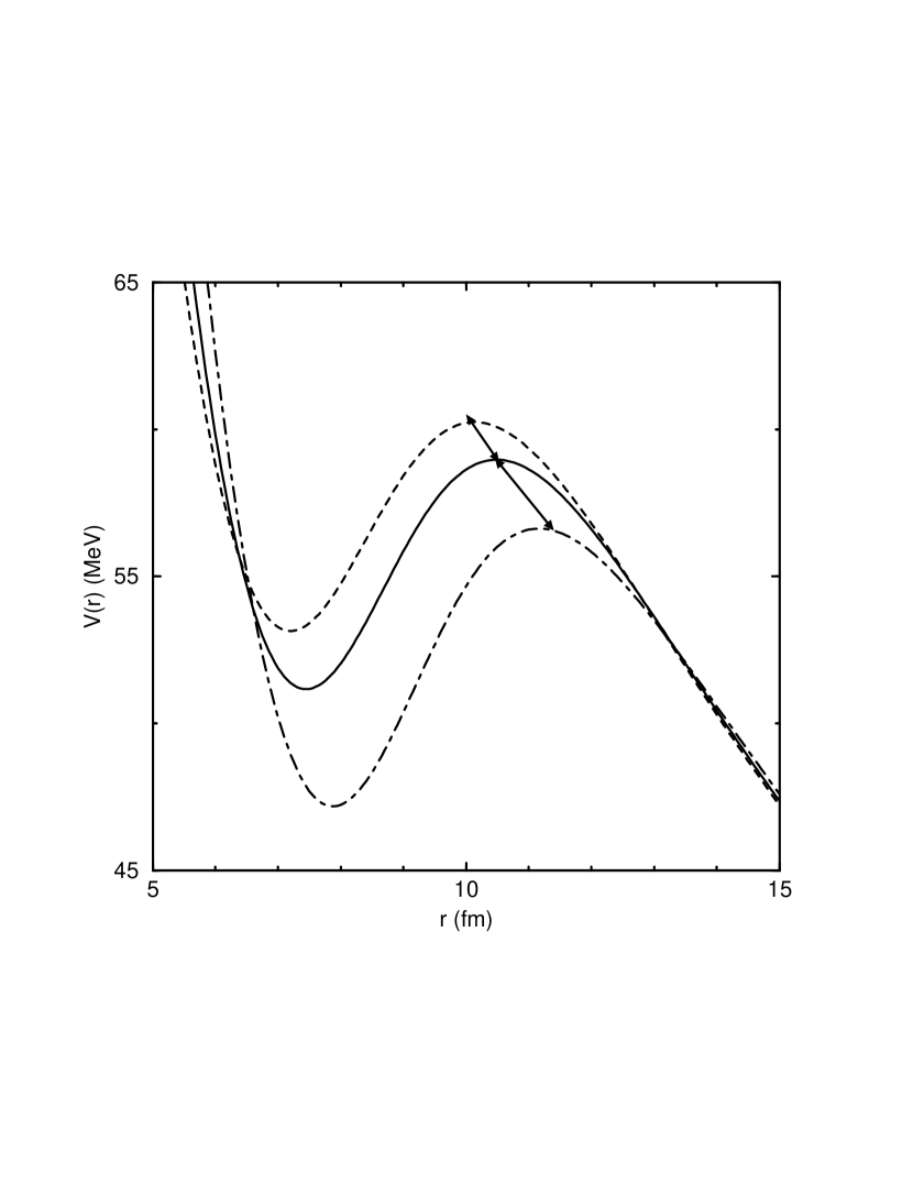
FIG. 4.: The solid curve is the total potential for the ¹⁶O+¹⁵⁴Sm system when the target is taken to be spherical. The dashed ($\lambda=-0.327$) and dot-dashed ($\lambda=0.613$) curves are the potentials for two-level approximation with $\beta=0.25$. The arrows show the shifts predicted for the barrier peaks by Eqs. (52) and (53).

FIG. 5.: The effective radius from a two-level calculation for the ¹⁶O+¹⁵⁴Sm system with $\beta=0.25$. The solid curve is calculated using the definition, Eq. (63), and the dot-dashed curve using Eq. (66), which assumes $\alpha$ is constant. For comparison, the dashed curve is the result for a spherical target.

FIG. 6.: $\rho_{0}$ extracted from fusion calculations using Eq. (68) for the ¹⁶O+¹⁵⁴Sm system with with quadrupole coupling strengths $v_{2}=0$, 0.13 and 0.26, respectively.

FIG. 7.: Comparison of average angular momenta calculated using Eq. (25) with a constant value (dashed curve) and Eq. (69) (solid curve) for $\rho_{0}$ to the values calculated by IBMFUS (points) for the ¹⁶O+¹⁵⁴Sm system with the quadrupole coupling strength $v_{2}=0.26$. The parameters used were $r_{0}=10.6$ fm, $\delta=1.22$ fm, $V_{B0}=59$ MeV, and $W=2.3$ MeV.

FIG. 8.: Average angular momenta data[2] for the system ¹⁶O+¹⁵⁴Sm. The solid curve shows the results using Eq. (71) and dashed curve those from IBMFUS[19]

REFERENCES

• [1] N. Rowley, G.R. Satchler, and P.H. Stelson, Phys. Lett. B 254 (1991) 25.
• [2] J.X. Wei, J.R. Leigh, D.J. Hinde, J.O. Newton, R.C. Lemmon, S. Elfstrom, J.X. Chen, and N. Rowley, Phys. Rev. Lett. 67 (1991) 3368.
• [3] J.R. Leigh, N. Rowley, R.C. Lemmon, D.J. Hinde, J.O. Newton, J.X. Wei, J.C. Mein, C.R Morton, S. Kuyucak, and A.T. Kruppe, Phys. Rev. C 47 (1993) R437.
• [4] R.C. Lemmon, J.R. Leigh, J.X. Wei, C.R Morton, D.J. Hinde, J.O. Newton, J.C. Mein, M. Dasgupta, and N. Rowley, Phys. Lett. B 316 (1993) 32.
• [5] C.R. Morton et al., Phys. Rev. Lett. 72 (1994) 4074.
• [6] A.M. Stefanini et al., Phys. Rev. Lett. 74 (1995) 864.
• [7] T. Izumoto, T. Udagawa, and B.T. Kim, Phys. Rev. C 51 (1995) 761.
• [8] H.J. Krappe and H. Rossner, in Low Energy Nuclear Dynamics, edited by Y. Oganessian et al. (World Scientific, Singapore, 1995), p. 329.
• [9] R. Vandenbosch, Ann. Rev. Nucl. Part. Sci. 42 (1992) 447.
• [10] A.B Balantekin and P.E. Reimer, Phys. Rev. C 33 (1986) 379.
• [11] A.B. Balantekin, S.E. Koonin, and J.W. Negele, Phys. Rev. C 28 (1983) 1565.
• [12] M. Dasgupta, A. Navin, Y.K. Agarwal, C.V.K. Baba, H.C. Jain, M.L. Jhingan, and A. Roy, Phys. Rev. Lett. 66 (1991) 1414; M. Dasgupta, A. Navin, Y.K. Agarwal, C.V.K. Baba, H.C. Jain, M.L. Jhingan, and A. Roy, Nucl. Phys. A 539 (1992) 351.
• [13] C.V.K. Baba, Nucl. Phys. A 553 (1993) 719c.
• [14] C.H. Dasso, H. Esbensen, and S. Landowne, Phys. Rev. Lett. 57 (1986) 1498; H. Esbensen and S. Landowne, Nucl. Phys. A 467 (1987) 136.
• [15] N. Rowley, J.R. Leigh, J.X. Wei, and R. Lindsay, Phys. Lett. B 314 (1993) 179.
• [16] J.R. Bennett and A.J. DeWeerd, Computer code IBMFUS, University of Wisconsin (1993).
• [17] F. Iachello and A. Arima, The interacting boson model (Cambridge, 1987).
• [18] A.B. Balantekin, J.R. Bennett, and S. Kuyucak, Phys. Rev. C 49 (1994) 1079.
• [19] A.B. Balantekin, J.R. Bennett, and S. Kuyucak, Phys. Lett. B 335 (1994) 295.
• [20] D. Ackermann, Acta Phys. Pol. B 26 (1995) 517.
• [21] M.A. Nagarajan, A.B. Balantekin, and N. Takigawa, Phys. Rev. C 34 (1986) 894.
• [22] J.D. Bierman, A.W. Charlop, D.J. Prindle, R. Vandenbosch, and D. Ye, Phys. Rev. C 48 (1993) 319.
• [23] M.W. Cole and R.H. Good, Phys. Rev. A 18 (1978) 1085.
Refer to caption